A Low-Cost Maximum Power Point Tracking System Based on Neural Network Inverse Model Controller


Abstract
:1. Introduction
2. PV System Model
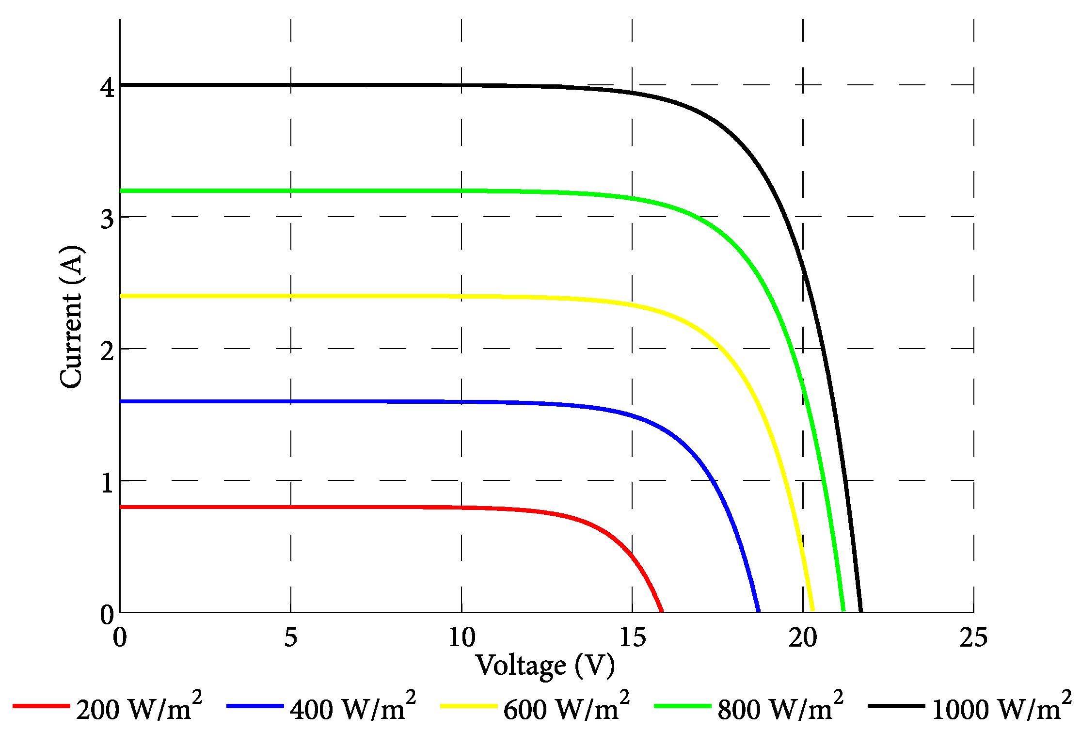
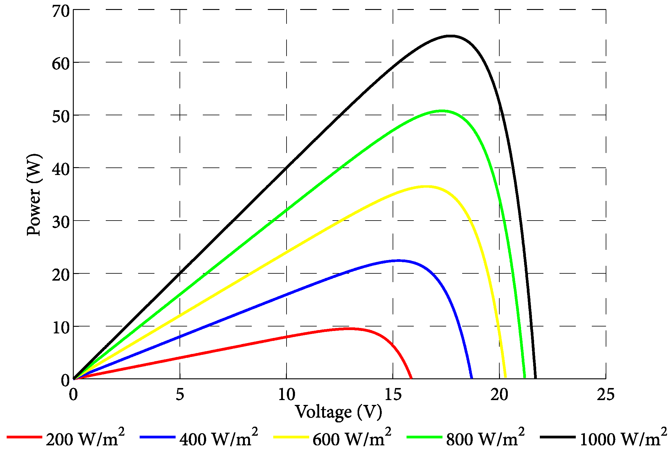
2.1. PV Module
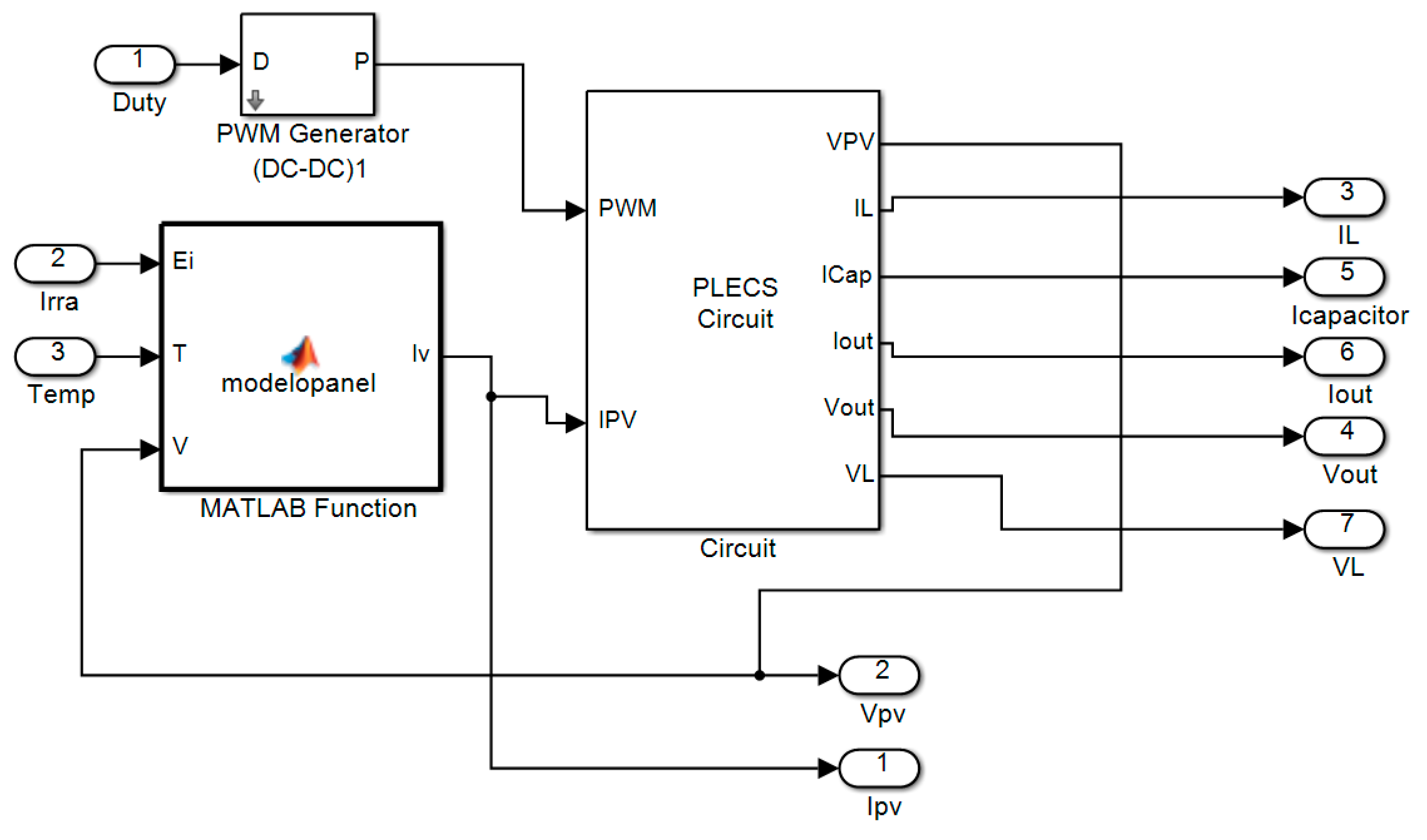
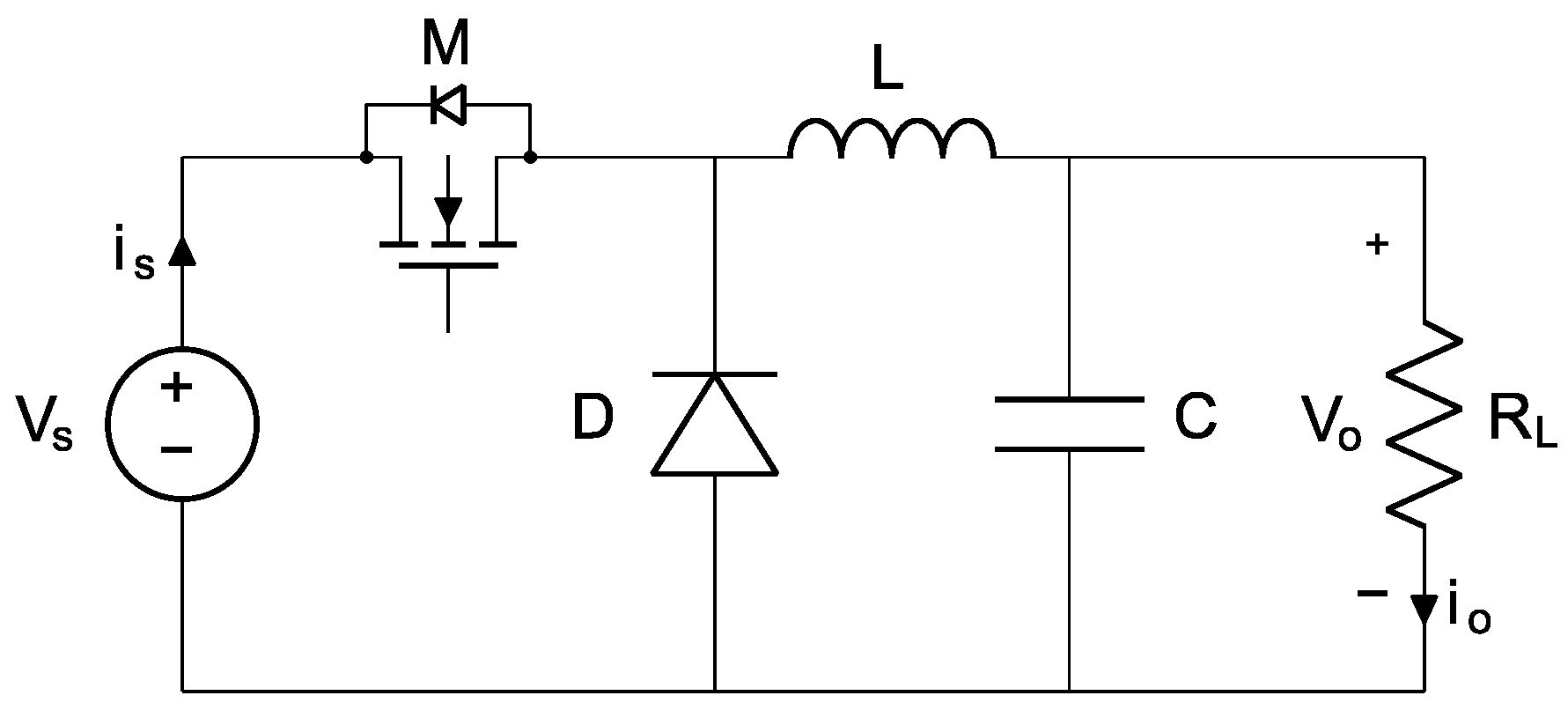
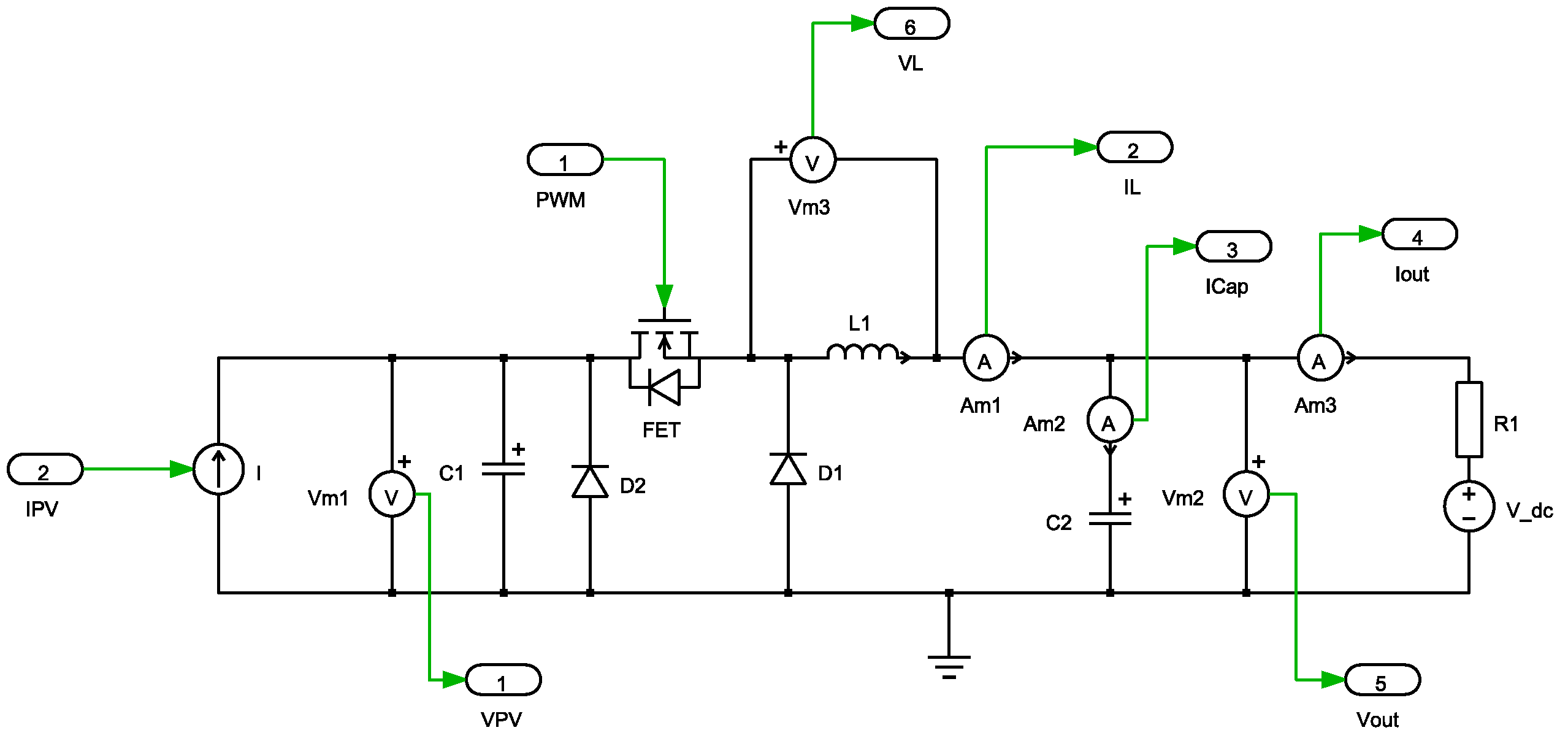
2.2. DC-DC Converter Model
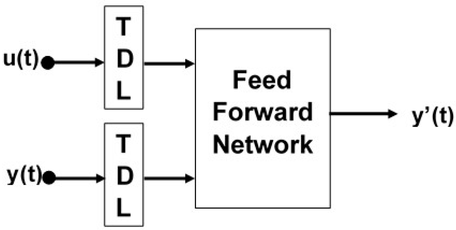
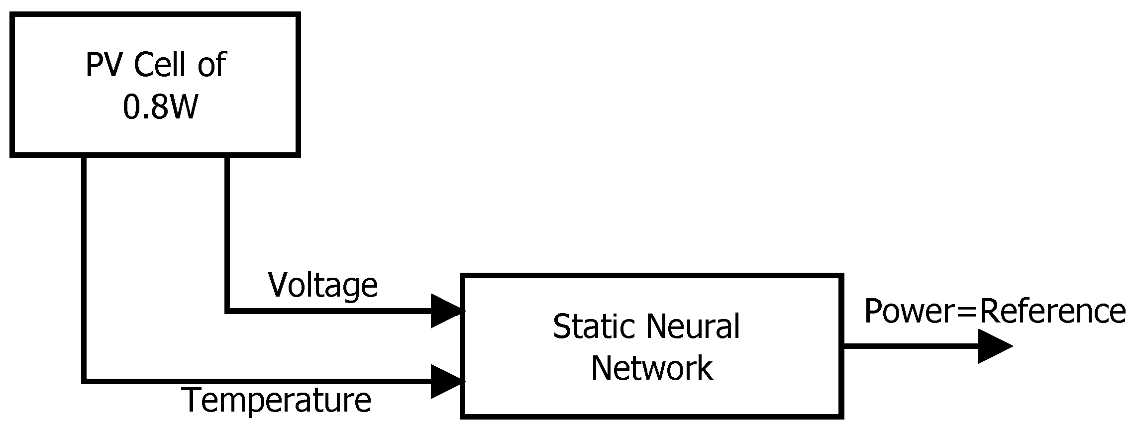
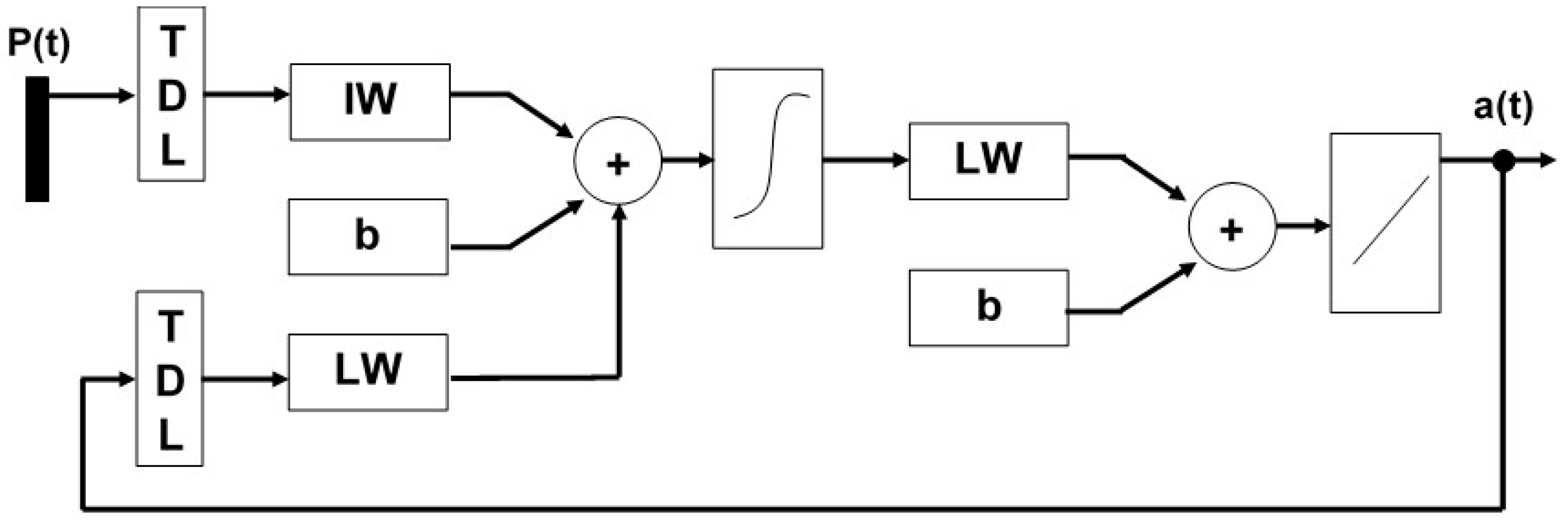
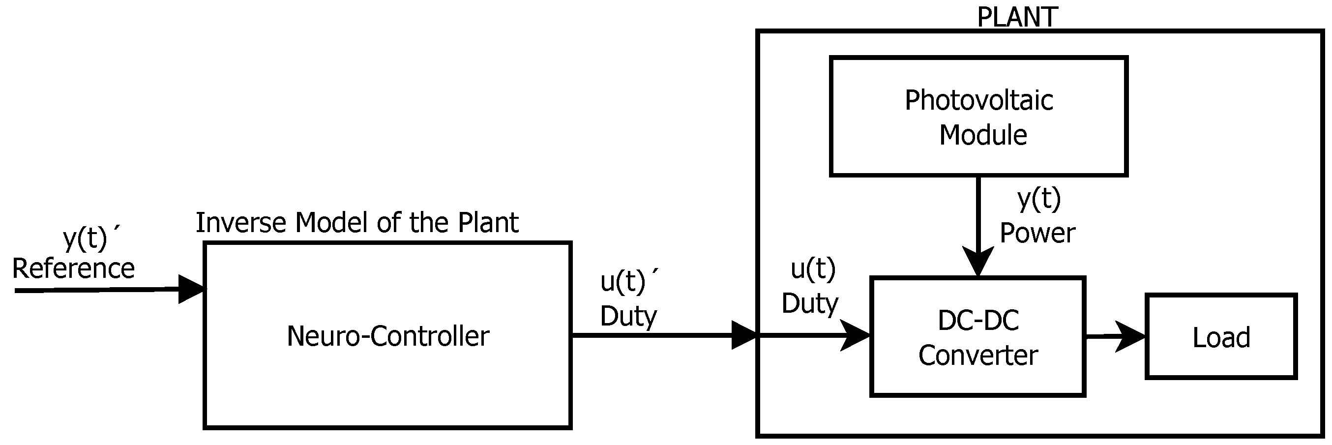
2.3. Neural Network Inverse Model Controller
2.4. Training of the Neural Network
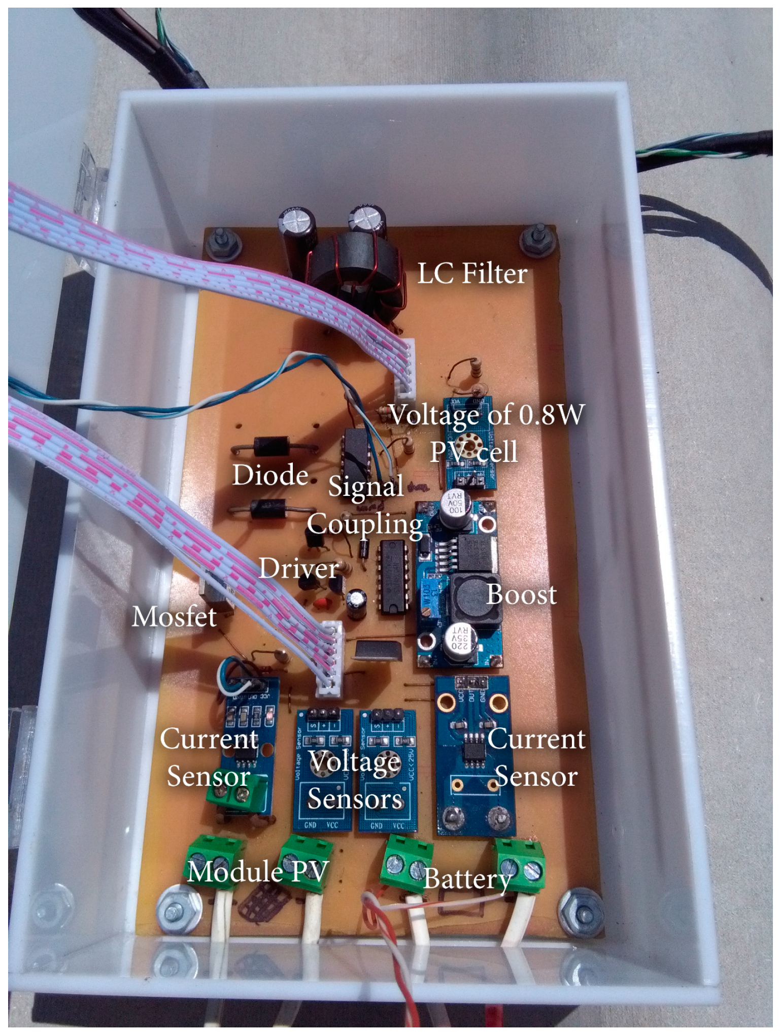
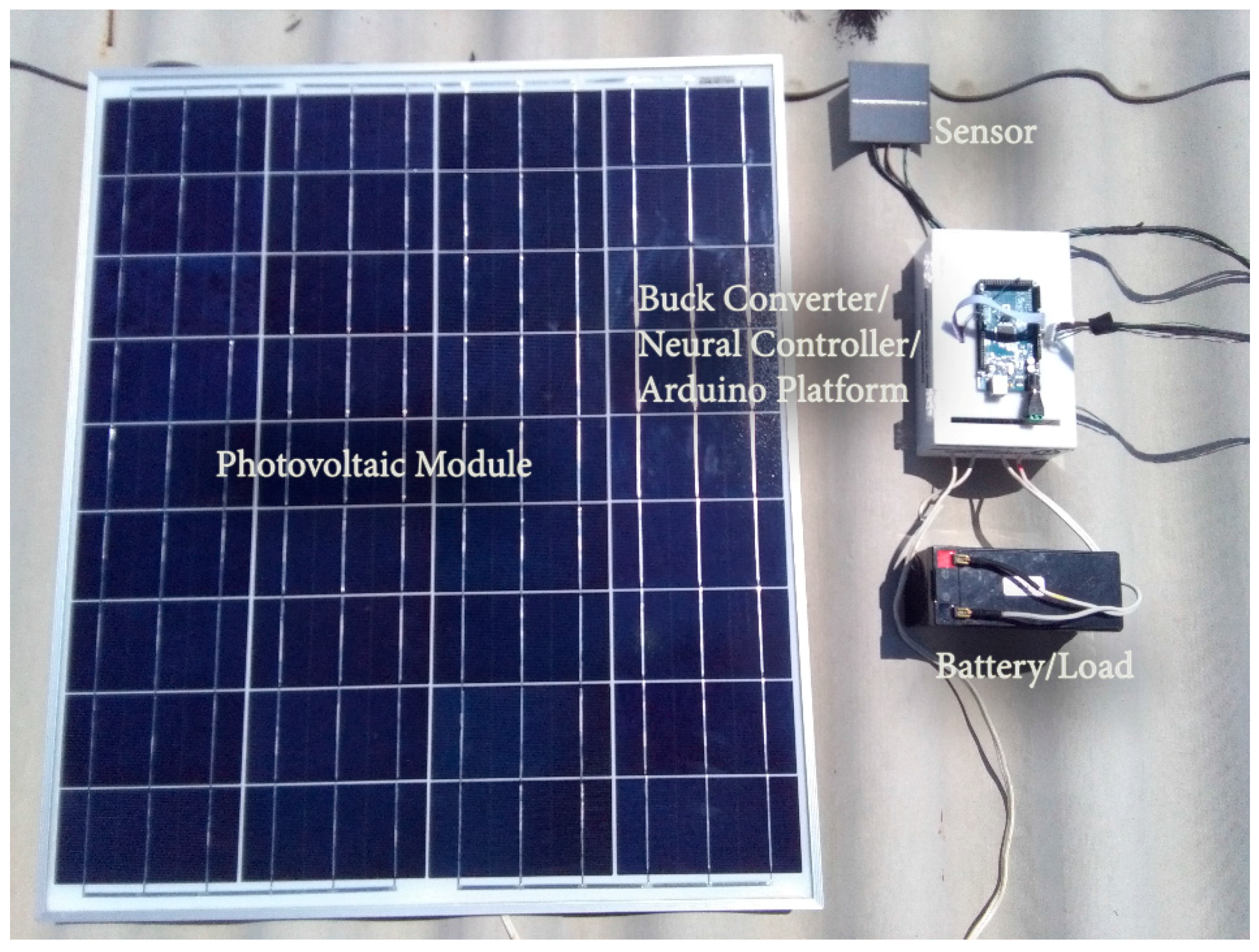
3. Implementation of the PV System
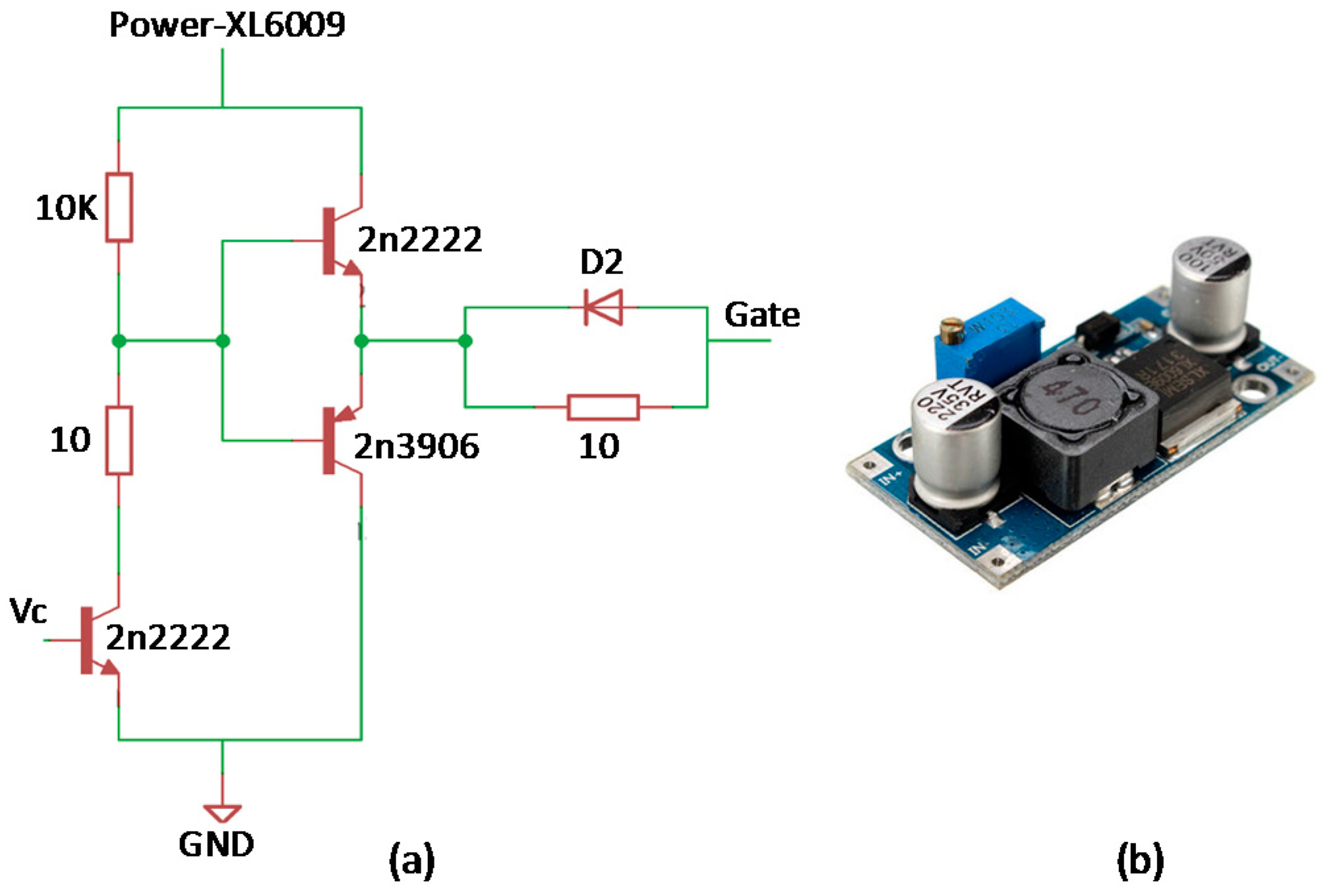
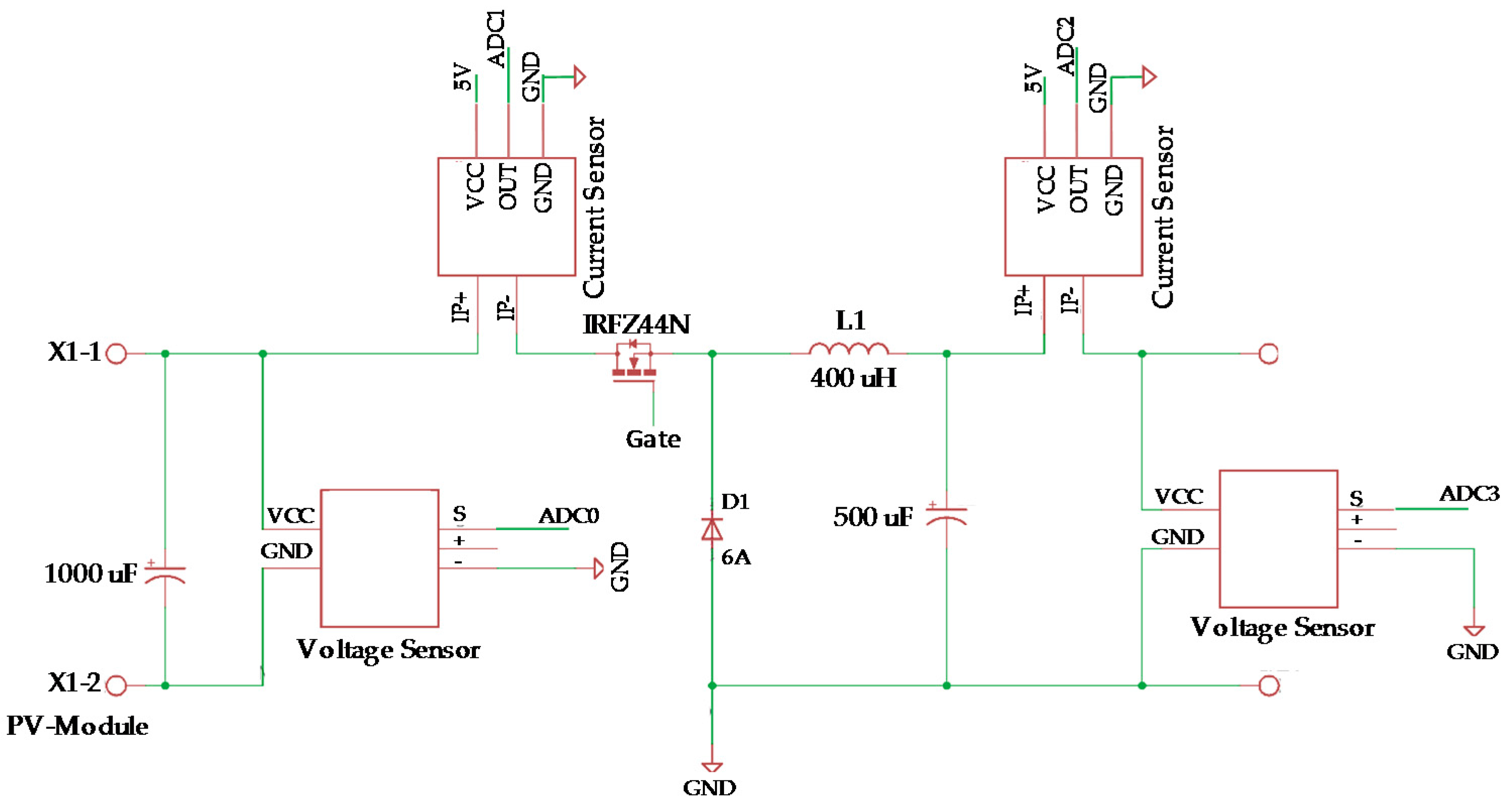
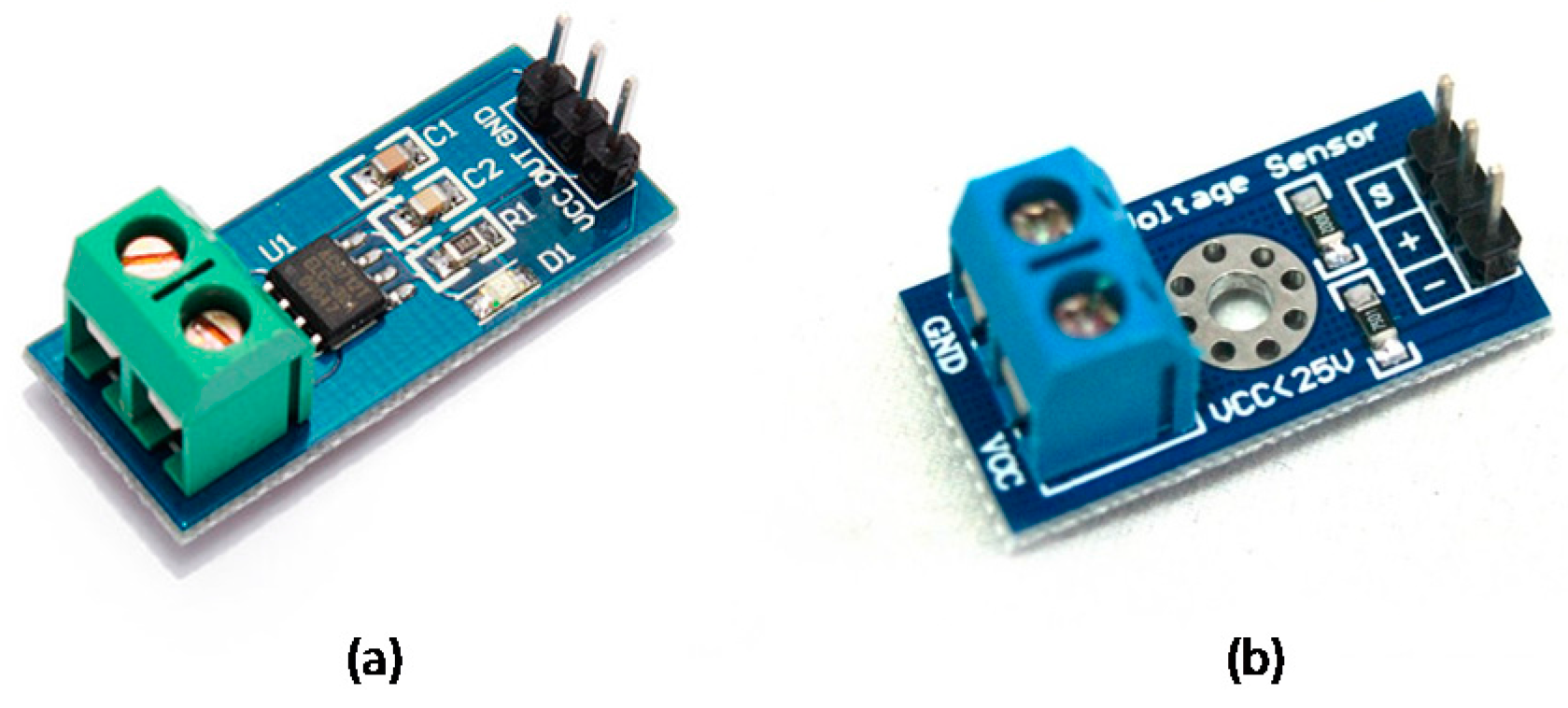
3.1. Buck Converter Implementation
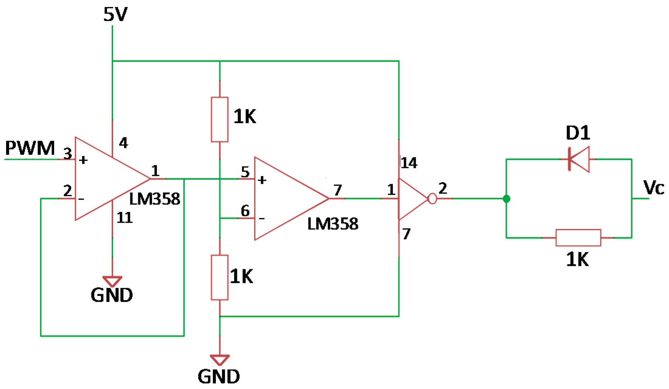
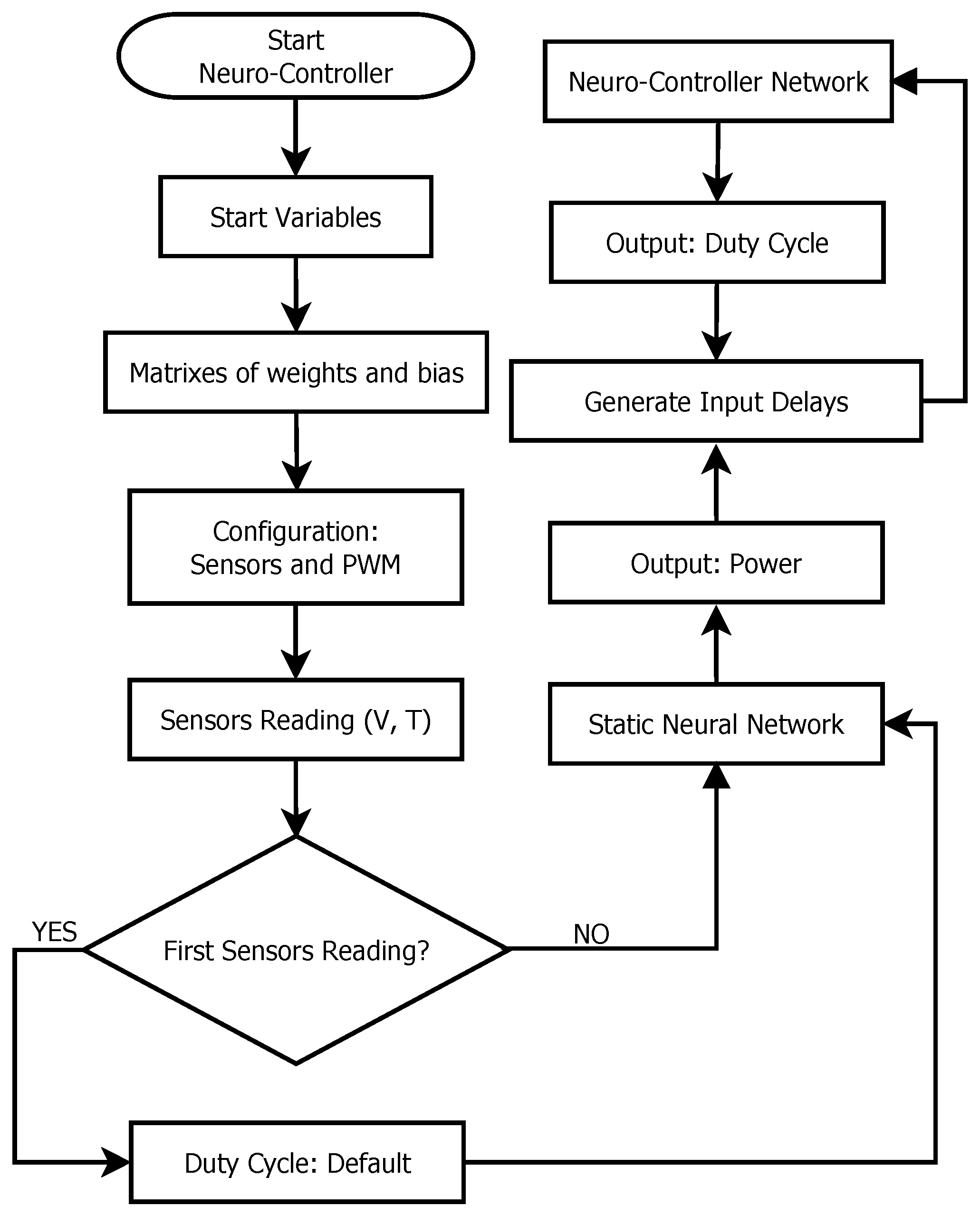
3.2. Neural Network Inverse Controller Implementation
4. Results and Discussion
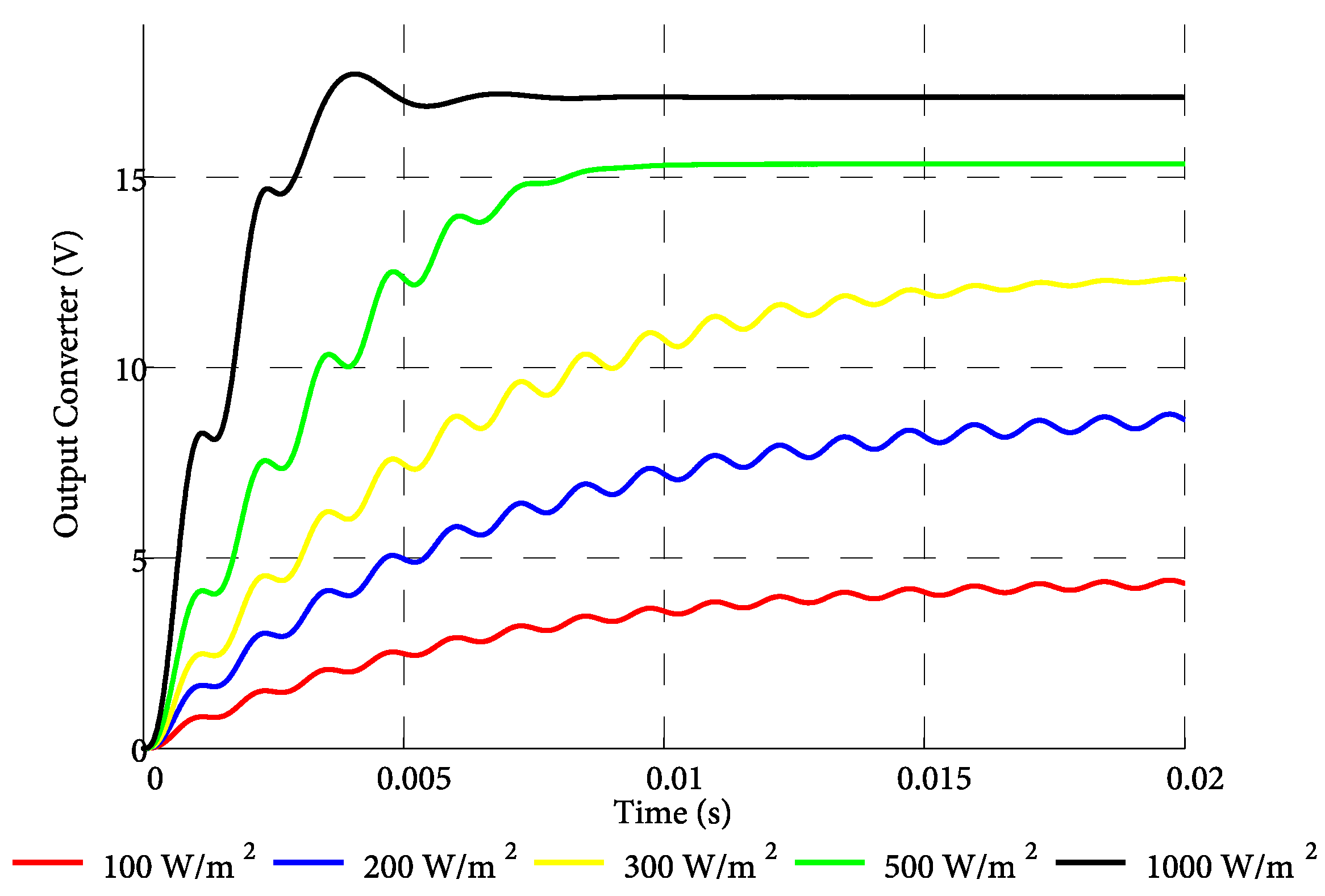
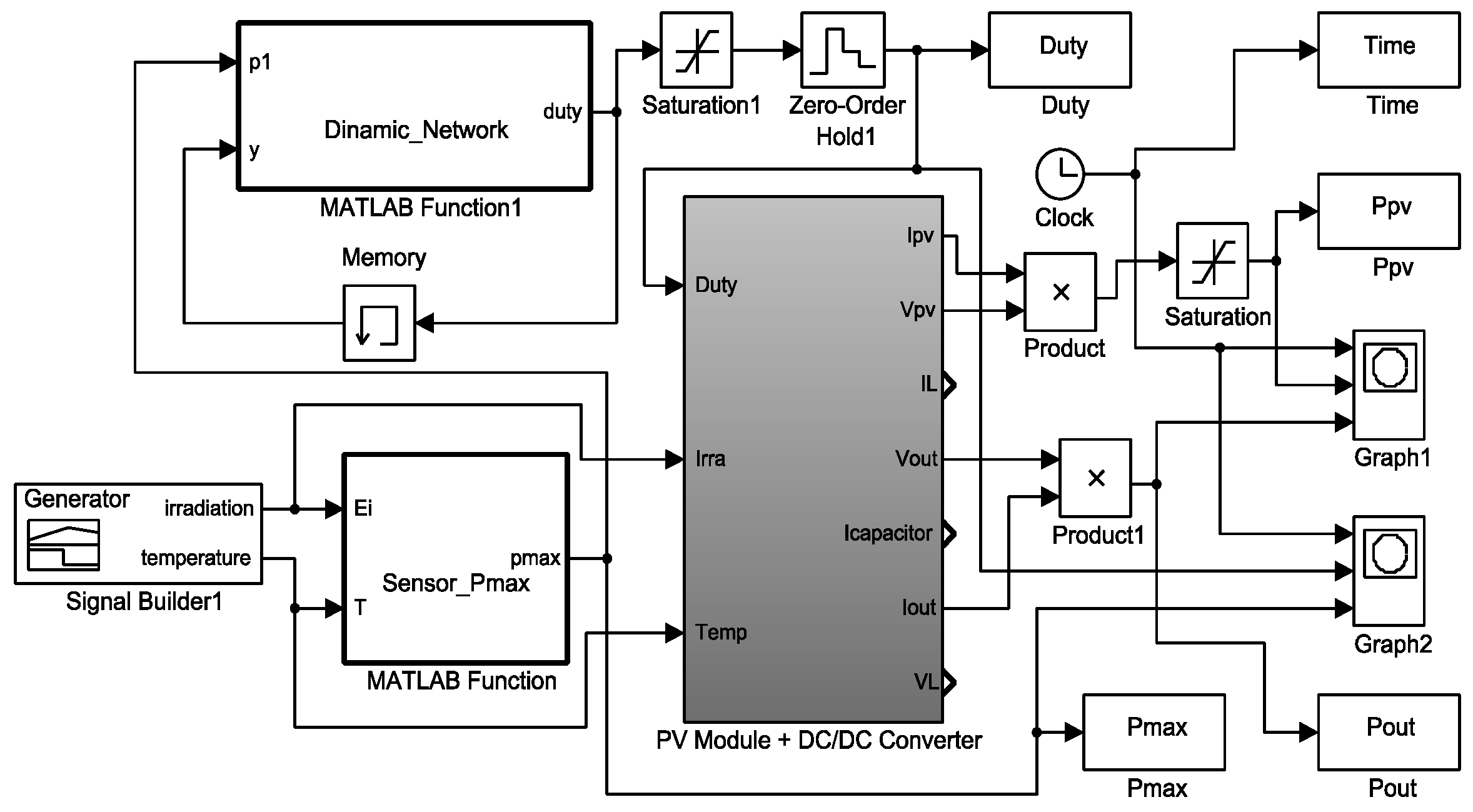
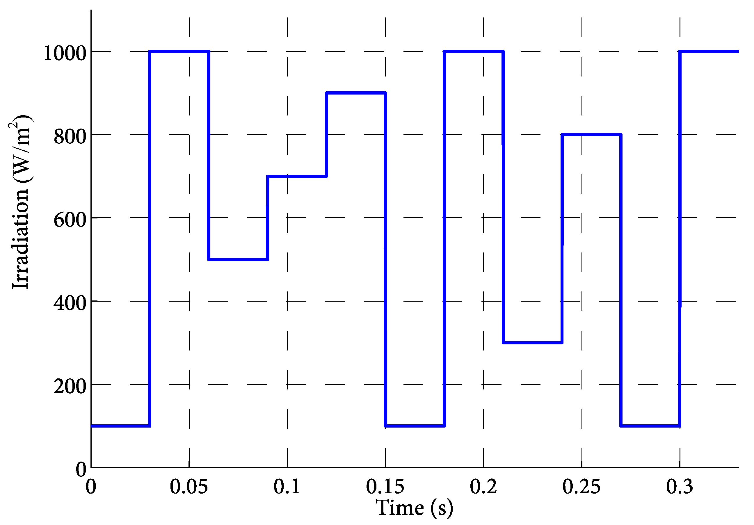
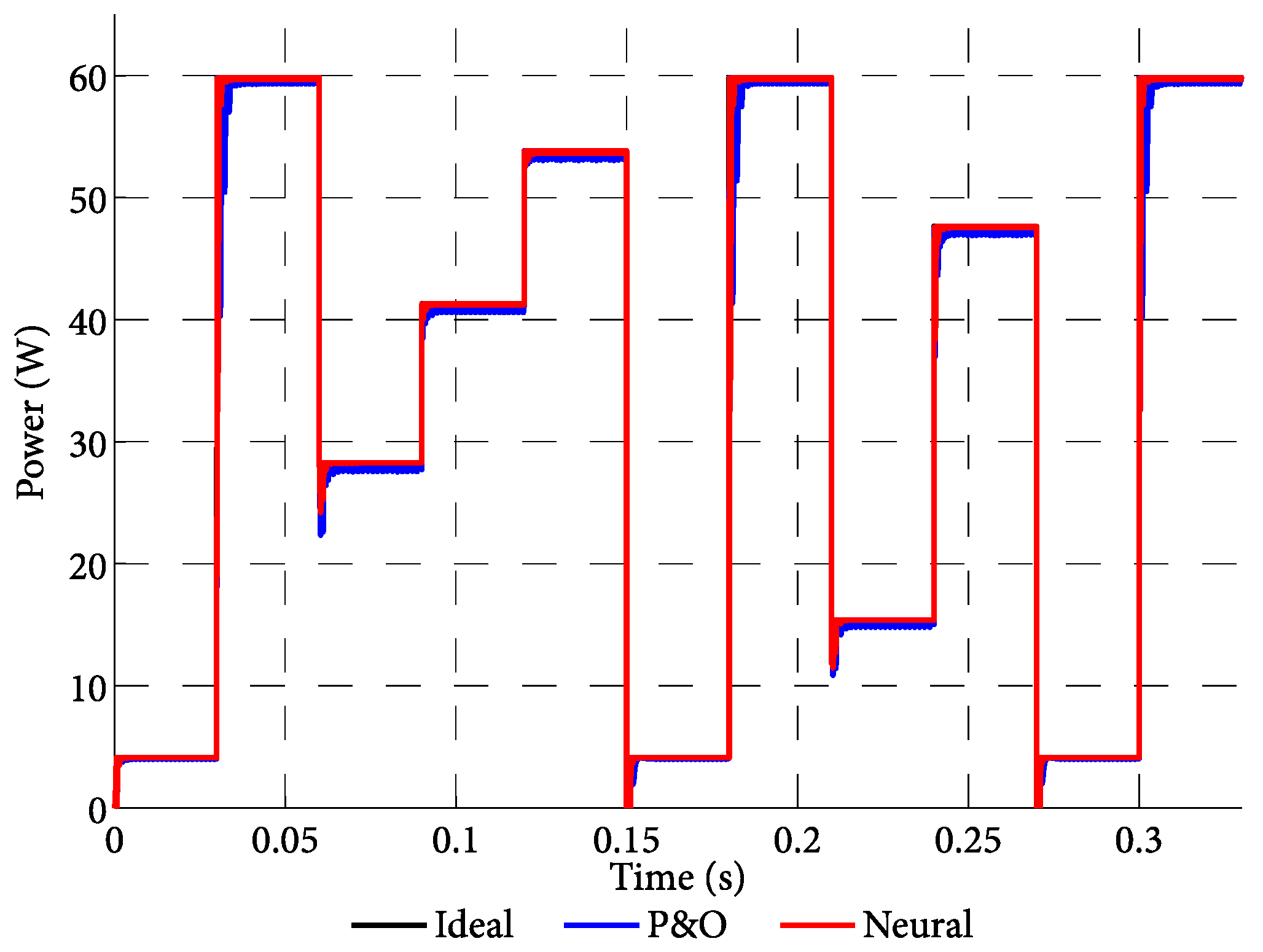
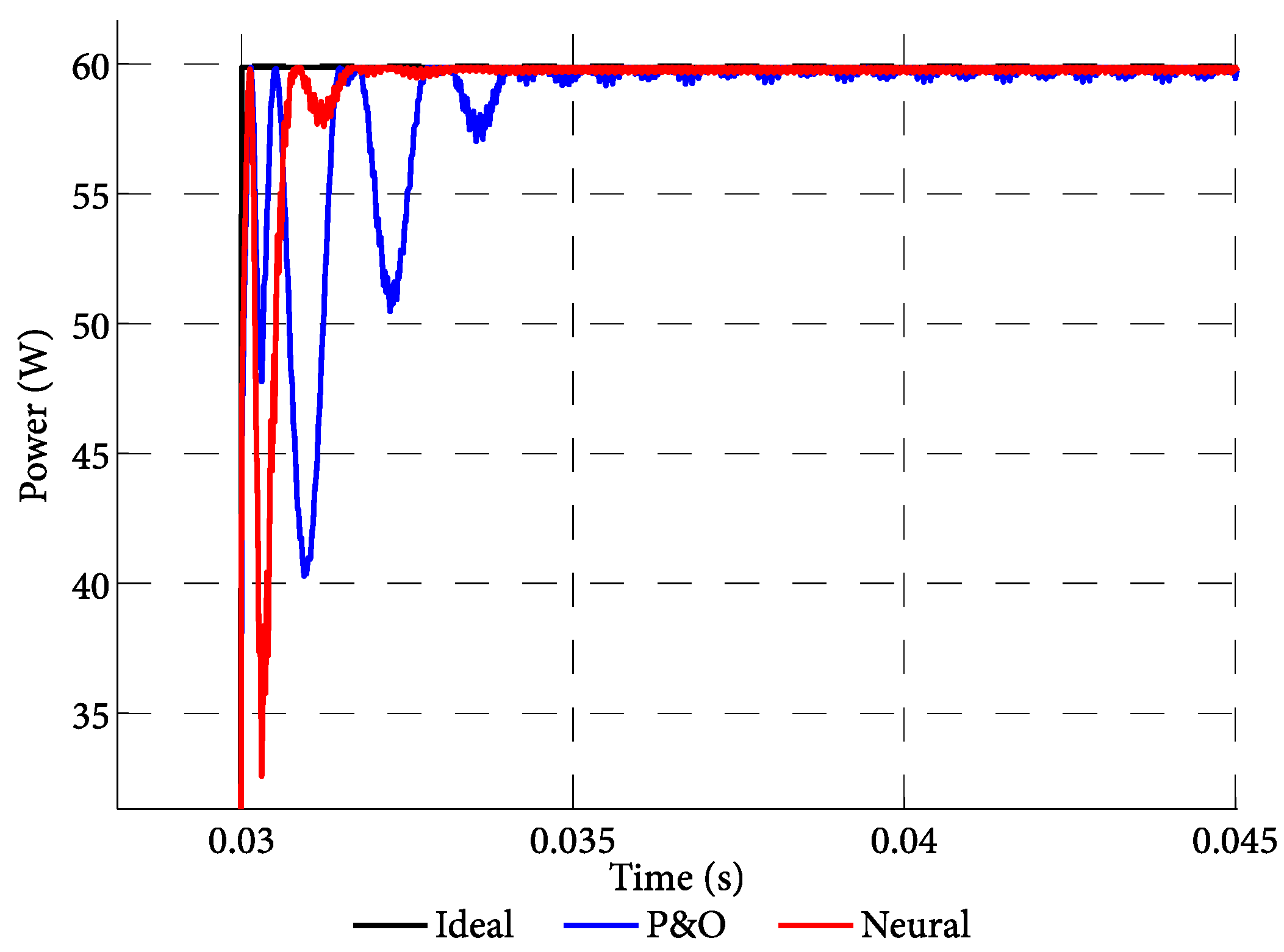
4.1. Simulation Results
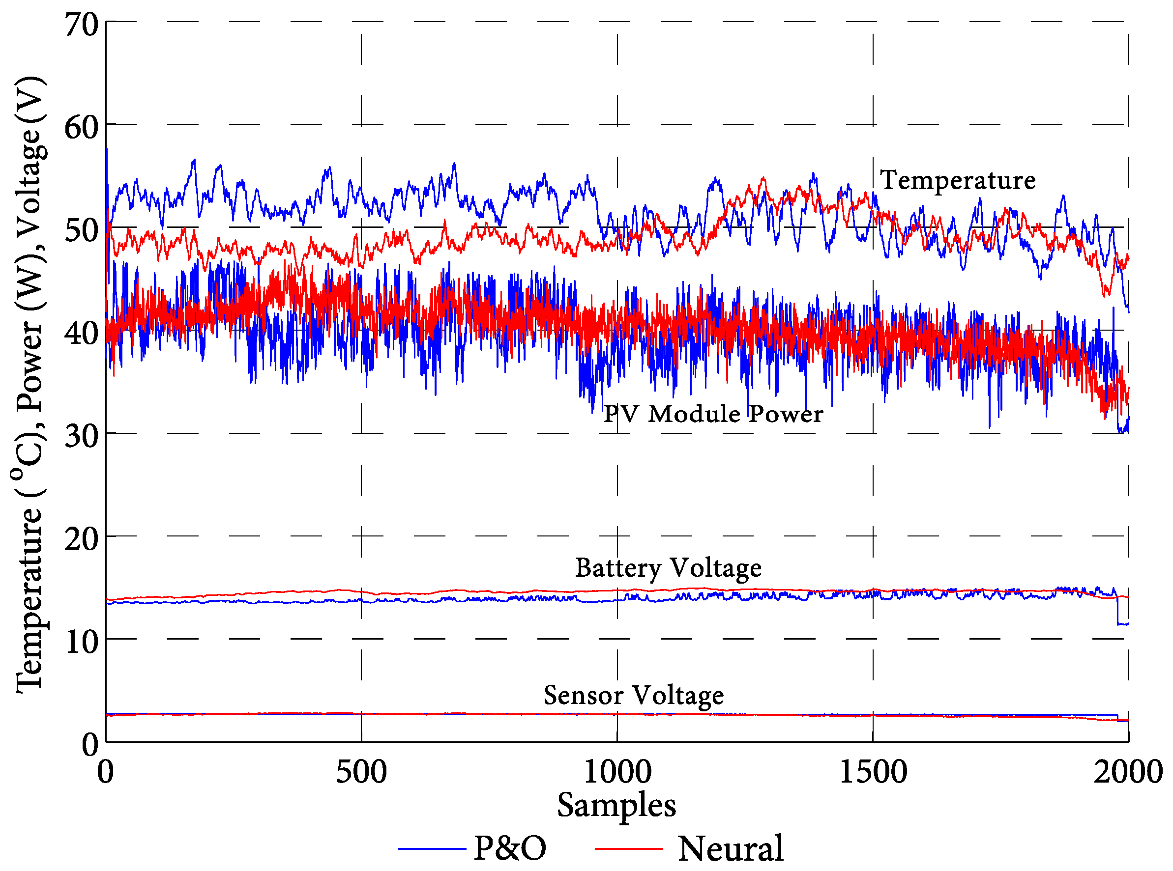
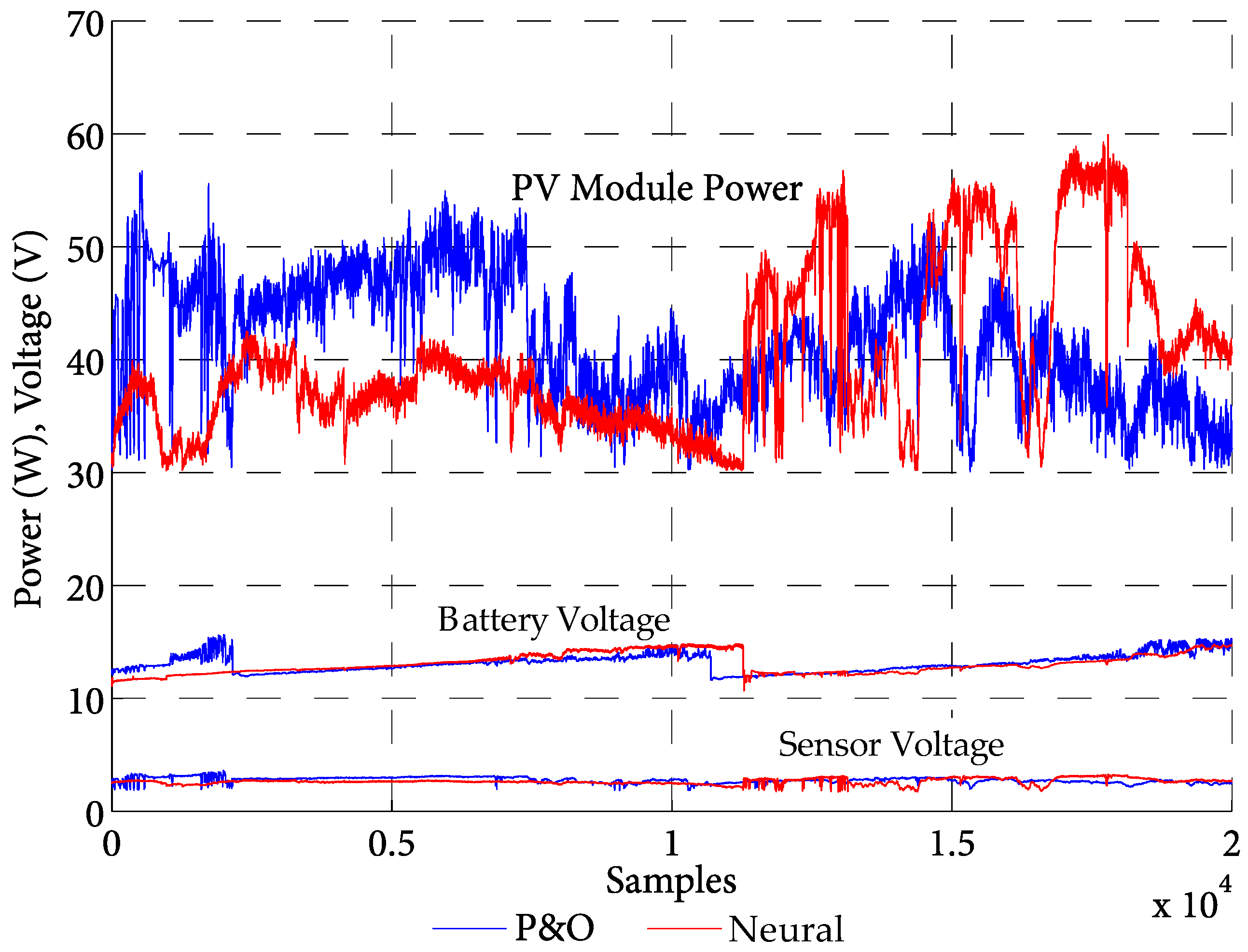
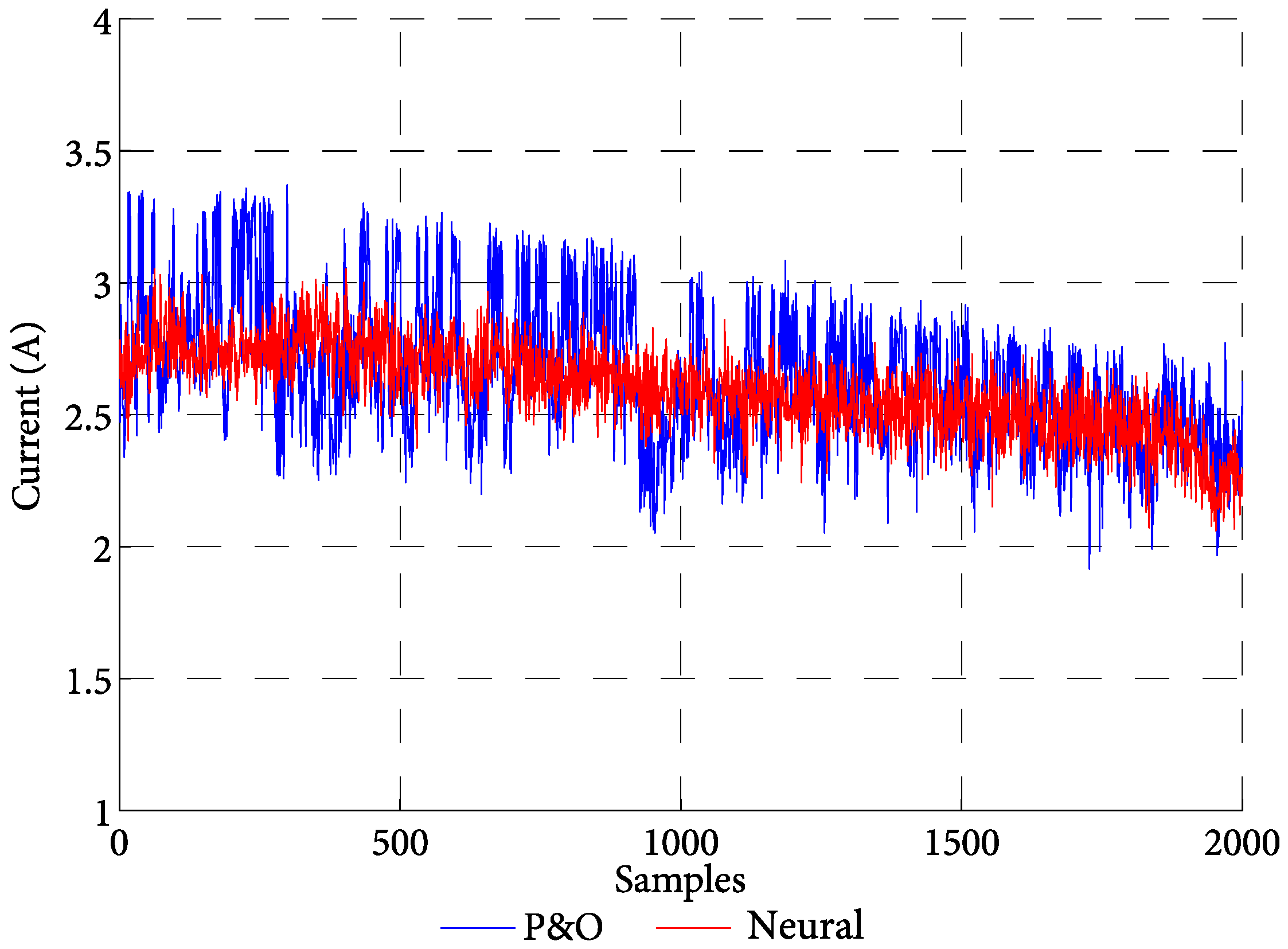
4.2. Implementation Results
5. Conclusions
Acknowledgments
Author Contributions
Conflicts of Interest
References
- Stamatescu, I.; Fagarasan, I.; Stamatescu, G.; Arghira, N.; Iliescu, S. Design and Implementation of a Solar Tracking Algorithm. Procedia Eng. 2014, 69, 500–507. [Google Scholar] [CrossRef]
- Vieira, R.; Guerra, F.; Vale, M.; Araújo, M. Comparative performance analysis between static solar panels and single-axis tracking system on a hot climate region near to the equator. Renew. Sustain. Energy Rev. 2016, 64, 672–681. [Google Scholar] [CrossRef]
- El Kadmiri, Z.; El Kadmiri, O.; Masmoudi, L.; Najib, M. A Novel Solar Tracker Based on Omnidirectional Computer Vision. J. Sol. Energy 2015, 2015, 1–6. [Google Scholar] [CrossRef]
- Fhong, J.; Rahim, N.; Al-Turki, Y. Performance of Dual-Axis Solar Tracker versus Static Solar System by Segmented Clearness Index in Malaysia. Int. J. Photoenergy 2013, 2013. [Google Scholar] [CrossRef]
- Robles, C.; Ospino, A.; Casas, J. Dual-Axis Solar Tracker for Using in Photovoltaic Systems. Int. J. Renew. Energy Res. 2017, 7, 137–145. [Google Scholar]
- Chen, F.; Yin, H. Fabrication and laboratory-based performance testing of a building-integrated photovoltaic thermal roofing panel. Appl. Energy 2016, 177, 271–284. [Google Scholar] [CrossRef]
- Lamnatou, C.; Mondol, J.; Chemisana, D.; Maurer, C. Modelling and simulation of Building-Integrated solar thermal systems: Behaviour of the coupled building/system configuration. Renew. Sustain. Energy Rev. 2015, 48, 178–191. [Google Scholar] [CrossRef]
- Buker, M.; Riffat, S. Building integrated solar thermal collectors—A review. Renew. Sustain. Energy Rev. 2015, 51, 327–346. [Google Scholar] [CrossRef]
- Rezaee, A. Maximum power point tracking in photovoltaic (PV) systems: A review of different approaches. Renew. Sustain. Energy Rev. 2016, 65, 1127–1138. [Google Scholar] [CrossRef]
- Saadsaoud, M.; Abbassi, H.; Kermiche, S.; Ouada, M. Study of Partial Shading Effects on Photovoltaic Arrays with Comprehensive Simulator for Global MPPT Control. Int. J. Renew. Energy Res. 2016, 6, 413–420. [Google Scholar]
- Filippini, M.; Molinas, M.; Oregi, E.O. A Flexible Power Electronics Configuration for Coupling Renewable Energy Sources. Electronics 2015, 4, 283–302. [Google Scholar] [CrossRef]
- Yaden, M.F.; Melhaoui, M.; Gaamouche, R.; Hirech, K.; Baghaz, E.; Kassmi, K. Photovoltaic System Equipped with Digital Command Control and Acquisition. Electronics 2013, 2, 192–211. [Google Scholar] [CrossRef]
- Sheik, S.; Devaraj, D.; Imthias, T. A novel hybrid Maximum Power Point Tracking Technique using Perturb & Observe algorithm and Learning Automata for solar PV system. Energy 2016, 112, 1096–1106. [Google Scholar] [CrossRef]
- Chen, Y.; Jhang, Y.; Liang, R. A fuzzy-logic based auto-scaling variable step-size MPPT method for PV systems. Sol. Energy 2016, 126, 53–63. [Google Scholar] [CrossRef]
- Hocksun, T.; Wu, X. Maximum power point tracking using a variable antecedent fuzzy logic controller. Sol. Energy 2016, 137, 189–200. [Google Scholar] [CrossRef]
- Nabipour, M.; Razaz, M.; Seifossadat, S.; Mortazavi, S. A new MPPT scheme based on a novel fuzzy approach. Renew. Sustain. Energy Rev. 2017, 74, 1147–1169. [Google Scholar] [CrossRef]
- Hassan, S.Z.; Li, H.; Kamal, T.; Arifoğlu, U.; Mumtaz, S.; Khan, L. Neuro-Fuzzy Wavelet Based Adaptive MPPT Algorithm for Photovoltaic Systems. Energies 2017, 10, 394. [Google Scholar] [CrossRef]
- Benyoucef, A.; Chouder, A.; Kara, K.; Silvestre, S.; Ait, O. Artificial bee colony based algorithm for maximum power point tracking (MPPT) for PV systems operating under partial shaded conditions. Appl. Soft Comput. 2015, 32, 38–48. [Google Scholar] [CrossRef]
- Pradhan, R.; Subudhi, B. Design and real-time implementation of a new auto-tuned adaptive MPPT control for a photovoltaic system. Int. J. Electr. Power 2015, 64, 792–803. [Google Scholar] [CrossRef]
- Hou, W.; Jin, J.; Zhu, C.; Li, G. A Novel Maximum Power Point Tracking Algorithm Based on Glowworm Swarm Optimization for Photovoltaic Systems. Int. J. Photoenergy 2016, 2016. [Google Scholar] [CrossRef]
- Titri, S.; Larbes, C.; Youcef, K.; Benatchba, K. A new MPPT controller based on the Ant colony optimization algorithm for Photovoltaic systems under partial shading conditions. Appl. Soft Comput. 2017, 58, 465–479. [Google Scholar] [CrossRef]
- Kofinas, P.; Dounis, A.; Papadakis, G.; Assimakopoulos, M. An Intelligent MPPT controller based on direct neural control for partially shaded PV system. Energy Build. 2015, 90, 51–64. [Google Scholar] [CrossRef]
- Aymen, M.; Romero, H.; Carmona, J.; Gomand, J. Maximum Power Point Tracking Using P&O Control Optimized by a Neural Network Approach: A Good Compromise between Accuracy and Complexity. Energy Procedia 2013, 42, 650–659. [Google Scholar] [CrossRef]
- Messalti, S.; Harrag, A.; Loukriz, A. A new variable step size neural networks MPPT controller: Review, simulation and hardware implementation. Renew. Sustain. Energy Rev. 2017, 68, 221–233. [Google Scholar] [CrossRef]
- Hu, Y.H.; Hwang, J.N. Handbook of Neural Network Signal Processing, 1st ed.; CRC Press: Seattle, WA, USA, 2001; pp. 12–13. [Google Scholar]
- Haykin, S. Neural Networks: A Comprehensive Foundation, 2nd ed.; Prentice Hall: Upper Saddle River, NJ, USA, 1998; pp. 23–28. [Google Scholar]
- Robles Algarín, C.; Callejas Cabarcas, J.; Polo Llanos, A. Low-Cost Fuzzy Logic Control for Greenhouse Environments with Web Monitoring. Electronics 2017, 6, 71. [Google Scholar] [CrossRef]
- Robles Algarín, C.; Taborda Giraldo, J.; Rodríguez Álvarez, O. Fuzzy Logic Based MPPT Controller for a PV System. Energies 2017, 10, 2036. [Google Scholar] [CrossRef]
- Gil, O. Modelado y Simulación de Dispositivos Fotovoltaicos. Master’s Thesis, Universidad de Puerto Rico, San Juan, Puerto Rico, 2008. [Google Scholar]
- Ortiz, E. Modeling and Analysis of Solar Distributed Generation. Ph.D. Thesis, Michigan State University, East Lansing, MI, USA, 2006. [Google Scholar]
- Robles, C.; Villa, G. Control del punto de máxima potencia de un panel solar fotovoltaico, utilizando lógica difusa. Telematique 2011, 10, 54–72. [Google Scholar]
- Hussain, M.; Ali, J.; Khan, M. Neural Network Inverse Model Control Strategy: Discrete-Time Stability Analysis for Relative Order Two Systems. Abstr. Appl. Anal. 2014, 2014, 1–11. [Google Scholar] [CrossRef]
- Hagan, M.T.; Demuth, H.B.; Beale, M.H.; De Jesús, O. Neural Network Design, 2nd ed.; Oklahoma State University: Stillwater, OK, USA, 2014; pp. 892–895. [Google Scholar]
- Medsker, L.R.; Jain, L.C. Recurrent Neural Networks: Design and Applications, 1st ed.; CRC Press: Seattle, WA, USA, 2001; pp. 142–145. [Google Scholar]


| Parameter | Value |
|---|---|
| Short-circuit current (Isc) | 4 A |
| Open circuit voltage (Voc) | 21.7 V |
| Voltage at Pmax (Vpmax) | 17.5 V |
| Current at Pmax (Ipmax) | 3.71 A |
| Temperature coefficient of voltage (Tcv) | 0.0802 V/°C |
| Temperature coefficient of current (Tci) | 0.0024 A/°C |
| Maximum voltage (Vmax) | 22.35 V |
| Minimum voltage (Vmin) | 18.44 V |
| Specifications | Values |
|---|---|
| Microcontroller | ATmega 2560 |
| Operating Voltage | 5 V |
| Digital I/O Pins | 54 (of which 15 provide PWM output) |
| Analog Input Pins | 16 |
| Clock Speed | 16 MHz |
| Flash Memory | 256 KB |
| SRAM-EEPROM | 8 KB–4 KB |
| Communication Interfaces | UART, SPI, I2C |
© 2018 by the authors. Licensee MDPI, Basel, Switzerland. This article is an open access article distributed under the terms and conditions of the Creative Commons Attribution (CC BY) license (http://creativecommons.org/licenses/by/4.0/).
Share and Cite
Robles Algarín, C.; Sevilla Hernández, D.; Restrepo Leal, D. A Low-Cost Maximum Power Point Tracking System Based on Neural Network Inverse Model Controller. Electronics 2018, 7, 4. https://doi.org/10.3390/electronics7010004
Robles Algarín C, Sevilla Hernández D, Restrepo Leal D. A Low-Cost Maximum Power Point Tracking System Based on Neural Network Inverse Model Controller. Electronics. 2018; 7(1):4. https://doi.org/10.3390/electronics7010004
Chicago/Turabian StyleRobles Algarín, Carlos, Deimer Sevilla Hernández, and Diego Restrepo Leal. 2018. "A Low-Cost Maximum Power Point Tracking System Based on Neural Network Inverse Model Controller" Electronics 7, no. 1: 4. https://doi.org/10.3390/electronics7010004
APA StyleRobles Algarín, C., Sevilla Hernández, D., & Restrepo Leal, D. (2018). A Low-Cost Maximum Power Point Tracking System Based on Neural Network Inverse Model Controller. Electronics, 7(1), 4. https://doi.org/10.3390/electronics7010004