Article

Effectiveness of Implicit Beamforming with Large Number of Antennas Using Calibration Technique in Multi-User MIMO System

1
Faculty of Engineering, Niigata University, Ikarashi 2-nocho 8050, Nishi-ku Niigata 950-218, Japan
2
Faculty of Engineering, Nippon Institute of Technology, 4-1 Gakuendai, Miyashiro-machi, Minamisaitama-gun, Saitama 345-8501, Japan
*
Author to whom correspondence should be addressed.
Electronics 2017, 6(4), 91; https://doi.org/10.3390/electronics6040091
Submission received: 12 September 2017 / Revised: 5 October 2017 / Accepted: 17 October 2017 / Published: 24 October 2017
(This article belongs to the Special Issue Smart Antennas and MIMO Communications)

Abstract

:
This paper examines the effectiveness of implicit beamforming (IBF), which enables transmission without channel state information (CSI) feedback in multi-user multiple-input multiple-output (MU-MIMO) systems with a large number of antennas. First, we explain why CSI feedback from terminal stations to the base station produces a very large overhead. A calibration technique is then introduced, which compensates for the difference between the complex amplitudes of the transmitters and receivers to facilitate CSI-feedback-free beamforming; this technique is called IBF. The efficacy of this calibration technique is demonstrated by measuring the amplitude and phase errors obtained using a 16-element array testbed and by performing a channel capacity evaluation. Finally, the throughput under IEEE802.11ac-based massive MIMO transmission, both with and without CSI feedback, is obtained in terms of the medium access control efficiency.

1. Introduction

The volume of data being transferred over wireless communication channels is almost doubling each year, owing to the popularity of smartphones and wireless local area networks (WLANs). Thus, high-speed data communication at speeds of faster than 10 Gbps will be required for future wireless communication systems [1,2,3]. In this context, multiple-input multiple-output (MIMO) systems have attracted significant attention, because they can improve the transmission rate (TR) within a limited frequency band [4,5]. Moreover, these systems have already been developed as commercial products in accordance with the Long Term Evolution (LTE) and IEEE802.11n standards [6,7]. In multi-user MIMO (MU-MIMO) systems, the channel capacity C is improved by employing a TR between a base station (BS) and multiple user equipment (UE) units, where the UE has a small number of antennas [8,9]. The MU-MIMO system has been incorporated into the LTE-Advanced and IEEE802.11ac standards [10].
With a view to further improving the frequency utilization of future wireless systems using MU-MIMO transmission, the concept of massive MIMO has recently been proposed [11,12]. In massive MIMO systems, the number of antennas at the BS is significantly larger than that of the UE and is also significantly larger than the number of UE units. Massive MIMO enables low-complexity signal processing, because the inter-user interference is easily mitigated by the high beamforming resolution [13]. Generally speaking, estimation of the channel state information (CSI) in MIMO/MU-MIMO systems [8] is essential [14,15]. However, when CSI feedback from the user terminals (UTs) to the BS is employed, a very large overhead occurs compared with the communication data, especially when there are a large number of antennas at the BS [16].
Thus, the countermeasure of implicit beamforming (IBF) has been proposed [17]. IBF exploits channel reciprocity in the time-division duplex (TDD) mode, that is, when the transmit frequency is identical to the receive frequency. Further, IBF can be used in WLAN systems. Because massive MIMO will be employed in small cell systems, the TDD mode should be used from the perspective of frequency utilization. However, it is necessary to calibrate the amplitude and phase errors between the branches of the array, because of individual differences in the radio frequency (RF) devices of the receivers and transmitters [18,19]. Thus, various automatic calibration methods for adaptive BS antennas that are well suited to TDD communication systems have been proposed in previous studies [20,21].We note that some of these methods allow the transmitter and receiver calibration values to be obtained automatically [20,21,22,23,24]. In recent research, the calibration method for massive antennas utilizing the channel reciprocity in a TDD system is proposed [25,26,27].
In this paper, we extend the calibration system described in [20,21] for applicability to MU-MIMO systems with a large number of antennas at the BS. Our testbed assumes a 16-element MIMO system. The amplitude and phase errors are evaluated on this testbed, and the efficacy of the calibration method is determined by examining the radiation pattern and C. Finally, the throughput performance obtained for MU-MIMO transmission under IBF with the developed calibration circuit is evaluated in terms of the medium access control (MAC) efficiency for IEEE802.11ac signals [28].
The remainder of this paper is organized as follows. The problems encountered with CSI feedback and the concept of IBF are introduced in Section 2. The calibration method, testbed, and its performance are described in Section 3. The radiation pattern and C given by the proposed calibration method are investigated in Section 4. In Section 5, the efficacy of the calibrated IBF is verified by examining the throughput performance while considering the MAC efficiency. Section 6 concludes the paper.

2. Problems with CSI Feedback and Overview of IBF

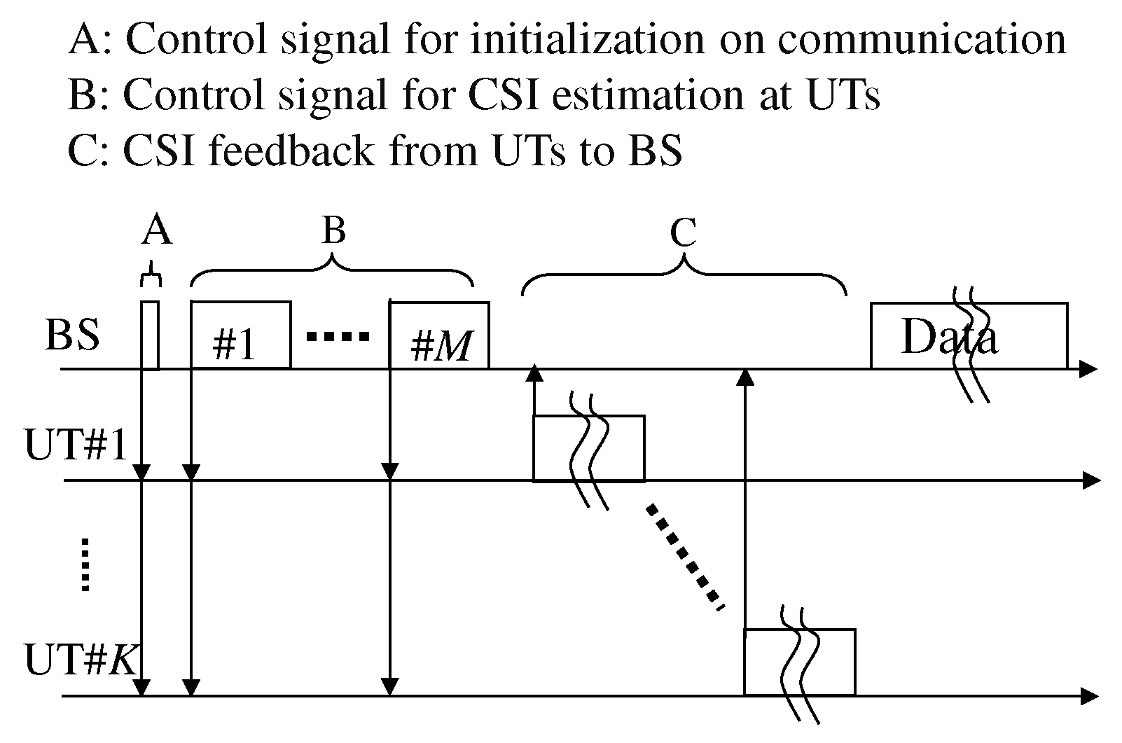
2.1. Problems with CSI Feedback
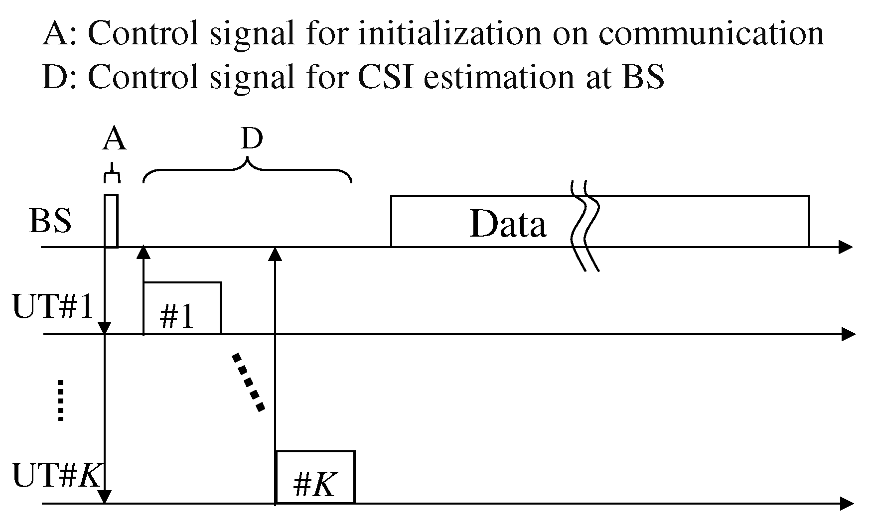
Figure 1 shows the frame format for a MU-MIMO system with CSI feedback. To initiate MU-MIMO transmission in the downlink channel, period A is required as a negotiation time for user selection. As shown in Figure 1, the CSI is estimated at the UTs using the information in period B, and the estimated CSI must be returned to the BS within period C. When considering the MU-MIMO system, the number of transmit antennas N T should be greater than or equal to the number of receive antennas multiplied by the number of users, that is., N R × N U . Therefore, period B incurs a large overhead. Although user scheduling is effective in the context of MU-MIMO transmission, as discussed in the previous section, period C incurs a very large overhead when user scheduling is considered. The influence of this CSI feedback overhead is discussed in Section 5.

2.2. IBF

Various CSI compression methods have been proposed, with the aim of reducing the overhead incurred by the transmission efficiency as a result of the CSI feedback [14,15]. However, even if CSI compression is employed, the CSI feedback continues to incur a significant overhead in cases for which a large number of antennas are located at the BS (e.g., for massive MIMO [11,12]) and/or when user scheduling is assumed.
To overcome this problem, beamforming without CSI feedback, or IBF, has been proposed [17]. Figure 2 shows the frame format for a MU-MIMO system when IBF is employed. It is apparent from this figure that the BS obtains the CSI directly from multiple UTs during period D, by utilizing the channel reciprocity between the transmission and reception in the TDD mode [17]. Moreover, because the number of UTs K is significantly less than the number of antennas at the BS M (Figure 1), the overhead during period B can be decreased using the frame format shown in Figure 1.
Originally, an adaptive array utilizing the channel reciprocity was proposed in order to avoid interference through use of the uplink channel [29,30]. Channel reciprocity means that the uplink and downlink share the same frequency band in TDD systems and that the receive weight created by the uplink channel can be utilized for the transmit weight [30]. In order to realize IBF, a calibration technique for the transmitters and receivers is essential [22,23,24].

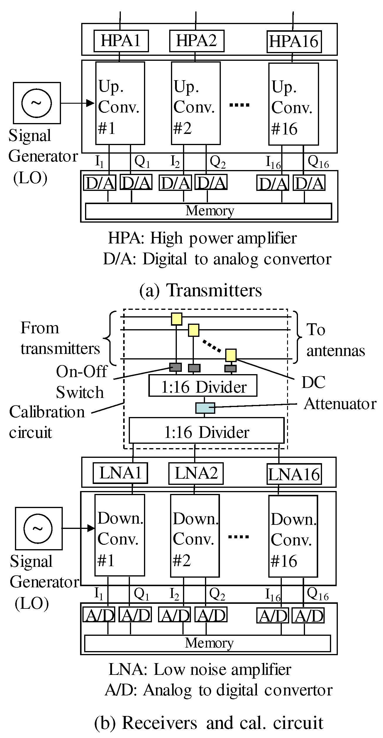
3. Calibration Circuit and Testbed for a Large Number of Antennas

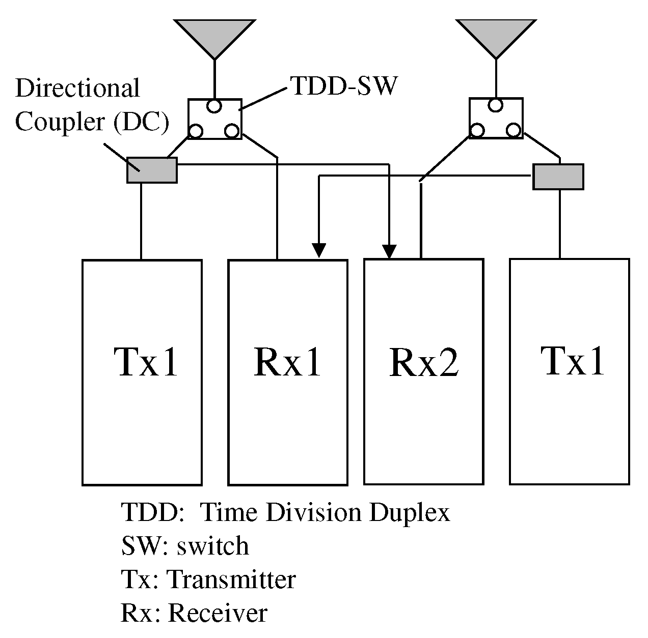
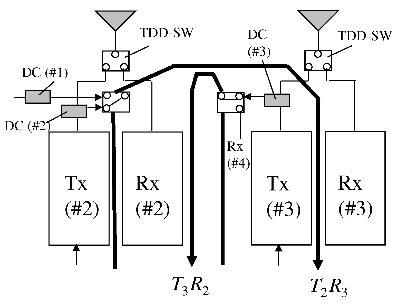
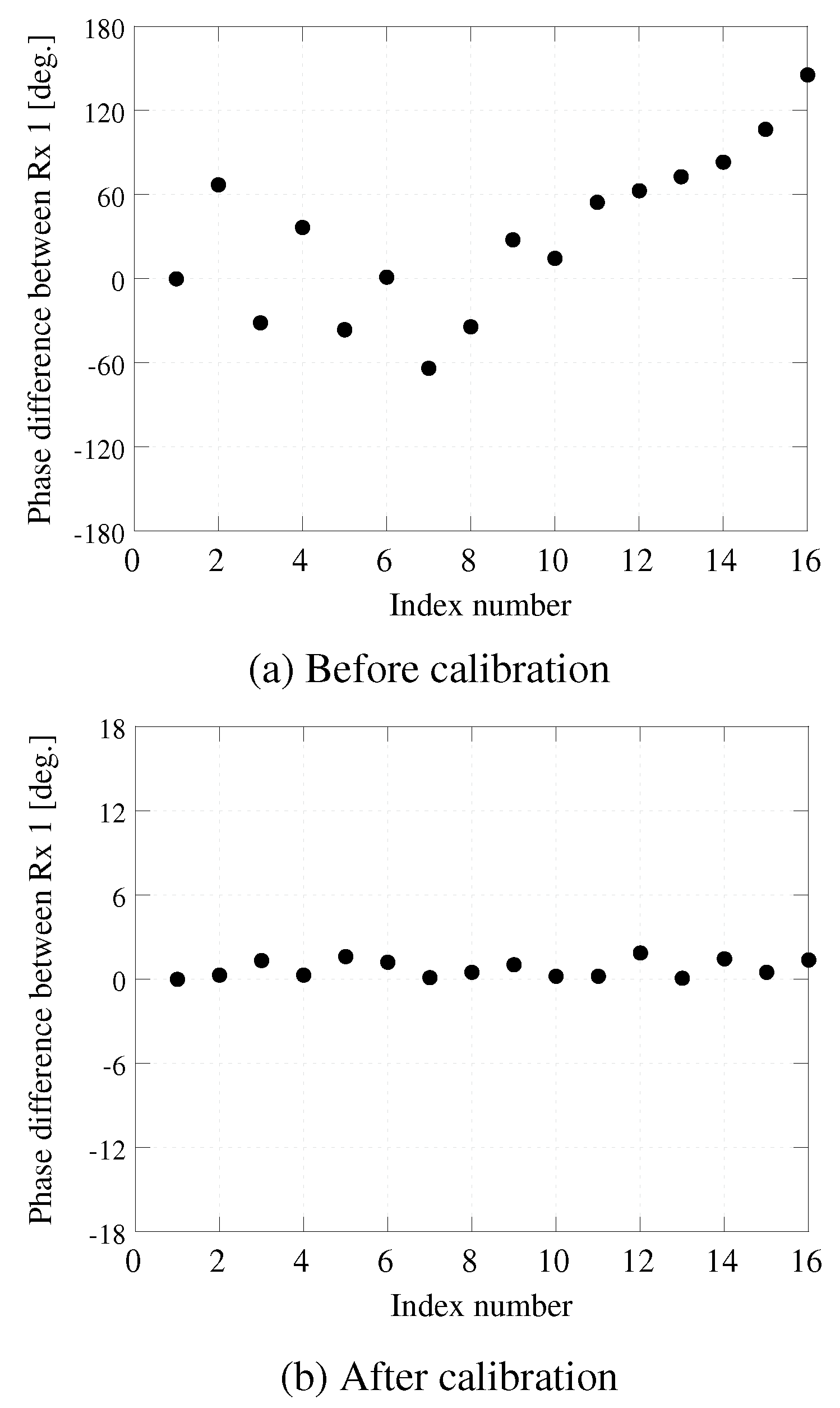
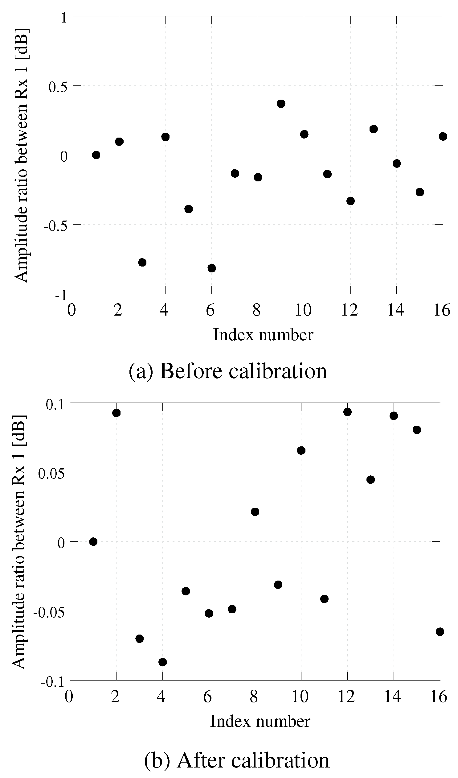
3.1. Basic Calibration Principle

To realize IBF, a calibration technique that compensates for the difference between the complex amplitudes of the transmitters and receivers at the BS is required [20]. Figure 3 shows the calibration circuit configuration. As shown in this figure, we obtain T i R j ( i = 1 , 2 , j = 2 , 1 ) , where T i and R j are the complex amplitudes of the transmitter and receiver, respectively. Because the calibration value required by the kth branch is T k / R k [20], the relative calibration values can be obtained from the circuit shown in Figure 3.
This concept can be extended to a large number of antennas [21], and the configuration for this case is shown in Figure 4. To enable the calibration of a large number of antennas using the hardware in Figure 3, switches with M branches are required when the number of elements is N. In contrast, the configuration in Figure 3 obtains the calibration values between two adjacent branches using a single-pole double-throw (SPDT) switch.
When T 1 R 2 and T 2 R 1 are obtained in advance, for example, using the configuration shown in Figure 3, the ratio between antennas # 1 and # 3 can be denoted as
D 3 , 1 = D 3 , 2 · D 2 , 1
= T 2 R 3 T 3 R 2 T 1 R 2 T 2 R 1
= T 1 R 3 T 3 R 1
From Equation (3), we can obtain the relative calibration value of antenna # 3 against antenna # 1 . Further, the ratio between antennas # k and # 3 is expressed as
D k , 1 = D k , k 1 · D k 1 , k 2 D 3 , 2 · D 2 , 1
= T k 1 R k T k + 1 R k T k 1 R k T k R k 1 T 2 R 3 T 3 R 2 T 1 R 2 T 2 R 1
= T 1 R k T k R 1

3.2. Testbed Configuration and Performance

Figure 5 shows the configuration of the testbed used to realize the calibration scheme. The main purpose of this testbed was to clarify the amplitude and phase-error characteristics for a 16-element MIMO system. T i R j ( i = 1 –16, j = 1 –16) can be obtained from a directional coupler (DC) and divider. The number of transmitters is 16, and 16 multi-user transmission is assumed at the maximum. The radio frequency is 2.425 GHz and the bandwidth is 50 MHz. This testbed can be utilized from 400 MHz to 6 GHz by changing the local oscillator in Figure 5.
Because the isolation between the transmitters and receivers is one of the key important issues when realizing the proposed calibration, on–off switches under DCs and an attenuator with between 1 and 16 dividers is implemented in our testbed.
Figure 6 and Figure 7 show the phase and amplitude errors at the receivers given by the testbed illustrated in Figure 5, both before and after calibration. In order to evaluate the basic performance, the continuous narrowband signal using minimum shift keying is transmitted, as shown in Figure 5. For a 10 ms interval, the transmit signals are switched for the calibration. The on–off switches in Figure 5 are used to switch the transmit signal from each transmitter.
For these measurements, the amplitude and phase errors yielded by the DCs and dividers in Figure 5 were measured in advance and removed. In addition, Figues Figure 6 and Figure 7 show the relative phase and amplitude errors of receiver k Txk against Tx1. As can be seen from Figure 6a, the phase error varied for each transmitter prior to calibration, and these values ranged from 60 ° to 150 ° . In contrast, when the calibration circuit in Figure 5 was applied, the phase errors could be eliminated, and these values were reduced to less than 1 . 5 ° . We note that, in addition, we have clarified the transmitter phase errors using the calibration circuit in Figure 5. Similarly, as can be seen from Figure 7, the amplitude errors could be reduced from ± 1 to ± 0.1 dB using the calibration circuit shown in Figure 5. Therefore, the effectiveness of the hardware in the testbed and the proposed calibration method has been verified.

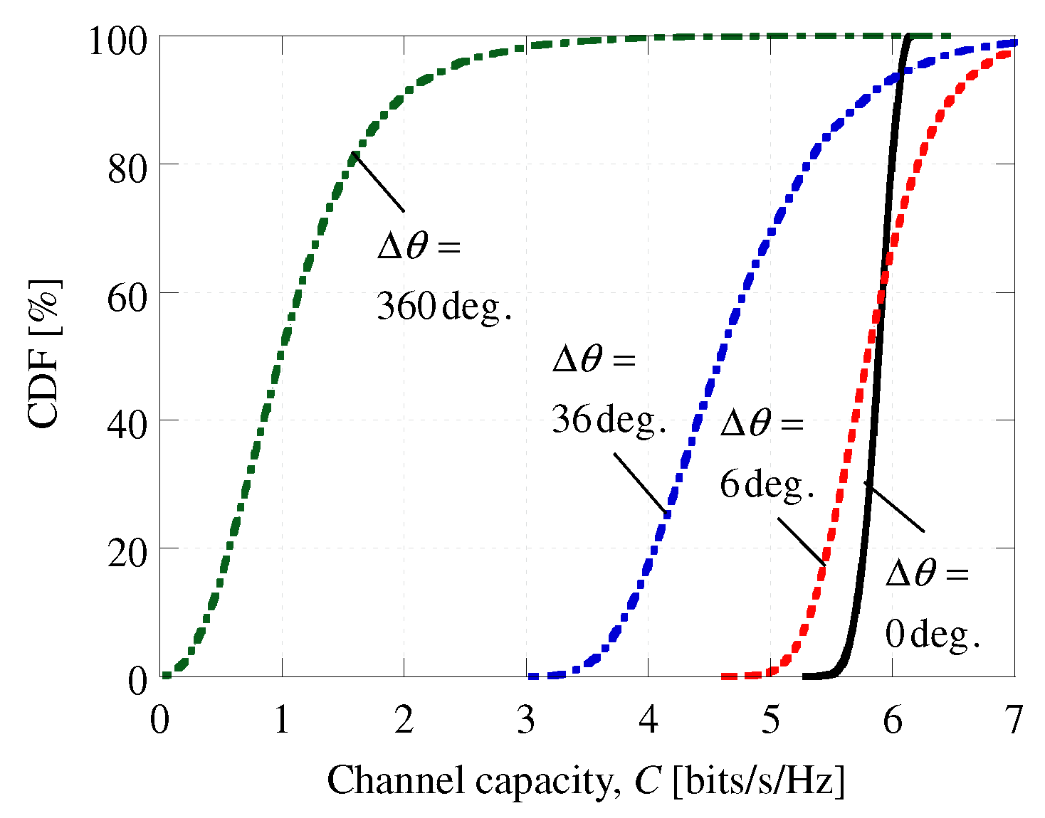
4. Channel Capacity and Radiation Pattern Given by Calibration Method

In this section, the performance is verified when considering the amplitude and phase errors shown in Figure 6 and Figure 7. The C and radiation pattern given by the calibration method have been evaluated via simulation, when considering the amplitude and phase errors shown in Figure 6 and Figure 7. This means that the correct transmission pattern cannot be created if there are amplitude and phase errors. In this evaluation, the ideal array factor is assumed and a mutual coupling effect between arrays is not considered. These effects should be evaluated in future work.
Table 1 lists the simulation parameters. In order to evaluate the C and radiation pattern directly using the testbed described in Section 3, we assume a 16-element linear array with half-wavelength spacing. The weights for the array combinations are obtained via maximum ratio combining (MRC). Propagation is assumed to occur over an additive white Gaussian noise (AWGN) channel, and the signal-to-noise power ratio (SNR) is 20 dB per antenna element. The amplitude and phase are given both with and without calibration errors, and the signal-to-interference-plus-noise power ratio (SINR) is calculated. The channel capacity is given by
C = log 2 ( 1 + SINR )
To verify the influence of the phase errors on C, the cumulative density function (CDF) of C for different phase errors and C as a function of the phase-error range Δ θ are plotted in Figure 8 and Figure 9, respectively; Δ θ is given by random numbers, and the number of trials is 10,000. We note that the C obtained for a CDF of 10% is plotted in Figure 9. Here, we have assumed that the desired signal and interference have directions of arrival (DoA) of θ d = 0 ° and θ i = 50 ° , respectively. As shown in Figure 8, C decreases even if Δ θ = 6 ° . Further, as can be seen from Figure 9, C decreases significantly in response to increased Δ θ . We find that Δ θ must be reduced to less than 2 ° ( 6 ° ) in order to ensure less than 1% (5%) degradation in C. As the calibration reduces Δ θ to less than 1.5 ° (Figure 6), we have, therefore, verified that the degradation in C is less than 1% under our proposed calibration circuit and scheme.
Next, we examine the radiation pattern given by the proposed calibration method using the testbed shown in Figure 5. Figure 10 shows the array patterns reflected by the phase errors in Figure 6. We note that the mutual coupling effect is not considered in Figure 10. The main beam directions in Figure 10a,b are 0 ° and 45 ° , respectively, using MRC. As can be seen from this figure, the sidelobe level is very high without calibration, especially in the 30 ° and 60 ° directions, because of the phase errors that occur in the absence of calibration. However, Figure 10 also shows that the ideal array pattern can be created when the calibration circuit is employed.
In Figure 11, the C with and without calibration is shown as a function of the difference in DoA; that is, θ i θ d , with θ d = 0 ° and θ i varying from 10 ° to 60 ° . The phase errors shown in Figure 6 are considered. When calibration is not employed, C decreases significantly compared to that obtained without phase errors, regardless of θ i . In contrast, the C with calibration is almost identical to that without phase errors (ideal). Because θ i = 30 ° is null when θ d = 0 ° with MRC, the C following calibration and without phase errors is 6 bit/s/Hz. It is clear that C decreases significantly when the null angle is considered for the interference.

5. Throughput Performance Using IEEE802.11ac Signals

To verify the efficacy of the IBF method with the proposed calibration technique, we conducted simulations using the IEEE802.11ac signal format. In this section, the performance is verified when considering the amplitude and phase errors shown in Figure 6 and Figure 7. The main simulation parameters are listed in Table 2. These simulations assumed path loss under the International Telecommunication Union (ITU) Radiocommunication Sector (ITU-R) model [31] and independent and identically distributed (i.i.d.) Rayleigh fading. The block diagonalization (BD) algorithm was employed for MU-MIMO transmission [8].
Table 3 illustrates the relationship between the transmission rate (TR) and SNR for IEEE802.11ac (40 MHz mode) [28]. Rmin is the minimum received power in Table 3.
As the eigenvalues given by the BD ( λ ˜ B D ( i ) ) determine the modulation scheme, the modulation schemes were selected on the basis of λ ˜ B D ( i ) / ( N T σ 2 ) for each trial, where σ 2 is the noise power. The SNR values listed in Table 3 were obtained when the bit error rate (BER) was less than 10 7 . The TRs were averaged using the results for each trial.
Figure 12 shows the average TR with respect to the transmit distance d between the BS and UT. We note that the calibration error was not considered here, and N T was set to 4, 8, or 16. A four-user MU-MIMO was assumed, with one antenna at the UT ( N R ). As can be seen from Figure 12, the TR and the service area were both increased by the transmit diversity effect when a larger number of antennas were located at the BS. For example, when N T was increased from 4 to 8 or 16 with d = 15 m , the TR increased by a factor of 2 or 2.5, respectively. Moreover, although the service area was only 35 m when N T = 4 , this increased to more than 50 m when N T = 8 or 16.
Figure 13 shows the average TR versus the transmit distance with and without calibration. We note that the overhead from control signals such as the CSI feedback (BR in Table 2) was not considered and that N T was 16. The calibration errors were taken from the phase-error results shown in Figure 6. In Figure 13, we can observe that the TR without calibration was less than that with calibration and less than that without calibration errors when d was 6 m. Moreover, when d was 15 rather than 6 m, the TR without calibration decreased from 600 to 360 Mbps. In contrast, the TR with calibration was almost identical to the ideal TR (without error). Hence, the calibration technique is essential for IBF.
Figure 14 shows the average throughput when the control signals in Table 2 are considered. The results with and without CSI feedback and calibration are given for a data size of 40,000 bytes. When calibration was adopted, the throughput was higher than that with CSI feedback, regardless of the transmit distance; thus, the IBF effect was ideally obtained. However, the throughput without calibration was lower than that with CSI feedback when d was greater than 13 m. Therefore, it is essential to apply IBF with the calibration technique for massive MIMO transmission.
Figure 15 shows the throughput improvement produced by the IBF with calibration R w / cal . for various data sizes. As can be seen from this figure, a large d and relatively small data size produce a higher throughput improvement for CSI feedback ( R w / cal . / R Exp . ; the latter is the throughput produced by explicit beamforming with CSI feedback). R w / cal . is superior to that without calibration R w / o cal . for larger data sizes. We can observe from Figure 15 that the throughput attained by IBF with calibration ( R w / cal . ) is twice that produced by explicit beamforming (with CSI feedback, R Exp . ) and 1.8 times that given by the IBF without calibration ( R w / o cal . ).

6. Conclusions

In this paper, we have demonstrated calibration for a system comprising a large number of BS antennas using IBF, and clarified the effectiveness of the proposed calibration method using a testbed that implements a 16 × 16 MIMO system. The phase-error range was reduced to less than 1.5 ° by the calibration technique, which is equivalent to a channel capacity degradation of less than 1%. Moreover, we have shown that the ideal array pattern can be created by the calibration circuit. In addition, the efficacy of IBF for various calibration errors (phase and amplitude) was verified by evaluating the throughput using IEEE802.11ac-based transmission with a large number of antennas. We found that IBF with the proposed calibration technique is essential for massive MIMO transmission in both the physical and MAC layers.

Acknowledgments

Part of this work was supported by the SCOPE #165004002 and KAKENHI, Grant-in-Aid for Scientific Research (B) (17H03262, 17H01738).

Author Contributions

This study was led by K. N. while T. H. and T. M. assisted with the computer simulations and measurements under the supervisions of H.Y.

Conflicts of Interest

The authors declare no conflict of interest.

References

  1. European Telecommunications Standards Institute. Feasibility Study for Further Advancement for E-UTRA (LTE-Advanced); 3GPP TS36.912 V9.1.0; European Telecommunications Standards Institute: Antibes, France, 2010. [Google Scholar]
  2. Thang, H. Summary of 3GPP TSG-RAN Workshop on Release 12 and Onward. In Proceedings of the 3GPP RAN Plenary, Ljubljana, Slovenia, November 2012. [Google Scholar]
  3. European Telecommunications Standards Institute. Scenarios and Requirements for Small Cell Enhancements for E-UTRAN; European Telecommunications Standards Institute: Antibes, France, October 2012. [Google Scholar]
  4. Foschini, G.J.; Gans, M.J. On limits of wireless communications in a fading environment when using multiple antennas. Wirel. Pers. Commun. 1998, 6, 311–335. [Google Scholar] [CrossRef]
  5. Paulaj, A.; Nabar, R.; Gore, D. Introduction to Space-Time Wireless Communications; Cambridge University Press: Cambridge, UK, 2003. [Google Scholar]
  6. Khandekar, A.; Bhushan, N.; Ji, T.; Vanghi, V. LTE advanced: Heterogeneous networks. In Proceedings of the 2010 European Wireless Conference (EW), Lucca, Italy, 12–15 April 2010; pp. 978–982. [Google Scholar]
  7. IEEE 802.11n. Available online: http://www.ieee802.org/11n/ (accessed on 7 September 2009).
  8. Spencer, Q.H.; Peel, C.B.; Swindlehurst, A.L.; Haardt, M. An introduction to the multi-user MIMO downlink. IEEE Commun. Mag. 2004, 42, 60–67. [Google Scholar] [CrossRef]
  9. Gesbert, D.; Kountouris, M.; Heath, R.W., Jr.; Chae, C.-B.; Salzer, T. Shifting the MIMO paradigm. IEEE Signal Process. Mag. 2007, 24, 36–46. [Google Scholar] [CrossRef]
  10. IEEE 802.11ac. Available online: http://www.ieee802.org/11ac/ (accessed on 7 January 2014).
  11. Larsson, E.G. Very Large MIMO Systems. In Proceedings of the 2012 IEEE International Conference on Acoustics, Speech and Signal Processing, Kyoto, Japan, 25–30 March 2012. [Google Scholar]
  12. Rusek, F.; Persson, D.; Lau, B.K.; Larsson, E.G.; Marzetta, T.L.; Edfors, O.; Tufvesson, F. Scaling up MIMO: Opportunities and challenges with very large MIMO. IEEE Signal Process. Mag. 2013, 30, 40–60. [Google Scholar] [CrossRef]
  13. Hoydis, J.; ten Brink, S.; Debbah, M. Massive MIMO in the UL/DL of cellular networks: How many antennas do we need? IEEE J. Sel. Areas Commun. 2013, 31, 160–171. [Google Scholar] [CrossRef] [Green Version]
  14. Love, D.J.; Heath, R.W., Jr. What is the value of limited feedback for MIMO channels. IEEE Commun. Mag. 2004, 42, 54–59. [Google Scholar] [CrossRef]
  15. Love, D.J.; Heath, R.W., Jr.; Lau, V.K.N.; Gesbert, D.; Rao, B.D.; Andrews, M. An overview of limited feedback in wireless communication systems. IEEE J. Sel. Areas Commun. 2008, 26, 1341–1365. [Google Scholar] [CrossRef]
  16. Hiraguri, T.; Nishimori, K. Survey of transmission methods and efficiency using MIMO technologies for wireless LAN systems. IEICE Trans. Commun. 2015, E98-B, 1250–1267. [Google Scholar] [CrossRef]
  17. Murakami, T.; Fukuzono, H.; Takatori, Y.; Mizoguchi, M. Multiuser MIMO with implicit channel feedback in massive antenna systems. IEICE Commun. Express 2013, 2, 336–342. [Google Scholar] [CrossRef]
  18. Litva, J.; Lo, T.K. Digital Beam Forming in Wireless Communication; Artech House: Norwood, MA, USA, 1996. [Google Scholar]
  19. Tsoulos, G.; McGeehan, J.; Beach, M. Space division multiple access (SDMA) field trials. 2. Calibration and linearity issues. IEE Proc. Radar Sonar Navig. 1998, 145, 79–84. [Google Scholar] [CrossRef]
  20. Nishimori, K.; Cho, K.; Takatori, Y.; Hori, T. Automatic calibration method using transmitting signals of an adaptive array for TDD systems. IEEE Trans. Veh. Technol. 2001, 50, 1636–1640. [Google Scholar] [CrossRef]
  21. Nishimori, K.; Cho, K.; Takatori, Y.; Hori, T. A novel configuration for realizing automatic calibration of adaptive array using dispersed SPDT switches for TDD systems. IEICE Trans. Commun. 2001, E84-B, 2516–2522. [Google Scholar]
  22. Hara, Y.; Yano, Y.; Kubo, H. Antenna array calibration using frequency selection in OFDMA/TDD Systems. In Proceedings of the IEEE GLOBECOM 2008 Global Telecommunications Conference, New Orleans, LA, USA, 30 November–4 December 2008. [Google Scholar]
  23. Zetterberg, P. Experimental investigation of TDD reciprocity-based zero-forcing transmit precoding. EURASIP J. Adv. Signal Process. 2011. [Google Scholar] [CrossRef]
  24. Shi, J.; Luo, Q.; You, M. An efficient method for enhancing TDD over the air reciprocity calibration. In Proceedings of the 2011 IEEE Wireless Communications and Networking Conference (WCNC), Cancun, Quintana Roo, Mexico, 28–31 March 2011; pp. 339–344. [Google Scholar]
  25. Vieira, J.; Rusek, F.; Tufvesson, F. Reciprocity calibration methods for massive MIMO based on antenna coupling. In Proceedings of the 2014 IEEE Global Communications Conference (GLOBECOM), Austin, TX, USA, 8–12 December 2014. [Google Scholar]
  26. Vieira, J.; Malkowsky, S.; Nieman, K.; Miers, Z.; Kundargi, N.; Liu, L.; Wong, L.; Öwall, V.; Edfors, O.; Tufvesson, F. A flexible 100-antenna testbed for Massive MIMO. In Proceedings of the 2014 Globecom Workshops (GC Wkshps), Austin, TX, USA, 8–12 December 2014. [Google Scholar]
  27. Bjornson, E.; Hoydis, J.; Kountouris, M.; Debbah, M. Massive MIMO Systems With Non-Ideal Hardware: Energy Efficiency, Estimation, and Capacity Limits. IEEE Trans. Inf. Theory 2014, 60, 7112–7139. [Google Scholar] [CrossRef] [Green Version]
  28. Wireless LAN Medium Access Control (MAC) and Physical Layer (PHY) Specifications. Available online: http://ieeexplore.ieee.org/document/6560345/ (accessed on 24 October 2017).
  29. Winter, J.H. Smart antennas for wireless systems. IEEE Pers. Commun. Mag. 1998, 5, 23–27. [Google Scholar] [CrossRef]
  30. Joham, M.; Utschick, W.; Nossek, J.A. Linear Transmit Processing in MIMO. IEEE Trans. Signal Process. 2005, 53, 2700–2712. [Google Scholar] [CrossRef]
  31. Recommendation ITU-R P. 1238-4, P Series. Available online: https://www.itu.int/rec/R-REC-P.1238/en (accessed on 24 October 2017).
Figure 1. Frame format for multi-user multiple-input multiple-output (MU-MIMO) transmission with channel state information (CSI) feedback.
Electronics 06 00091 g001
Figure 2. Frame format of multi-user multiple-input multiple-output (MU-MIMO) without channel state information (CSI) feedback.
Electronics 06 00091 g002
Figure 3. Basic circuit configuration of calibration method.
Electronics 06 00091 g003
Figure 4. Calibration circuit for a large number of base station (BS) antennas. Tx: Transmitter. Rx: Receiver.
Electronics 06 00091 g004
Figure 5. Testbed configuration: (a) Transmitters, and (b) Receivers and calibration circuit.
Electronics 06 00091 g005
Figure 6. Phase errors of Txk against Tx # 1 : (a) without, and (b) with calibration.
Electronics 06 00091 g006
Figure 7. Amplitude errors of Txk against Tx # 1 : (a) without, and (b) with calibration.
Electronics 06 00091 g007
Figure 8. Cumulative density function (CDF) of C for different Δ θ .
Electronics 06 00091 g008
Figure 9. C vs. Δ θ , with cumulative density function (CDF) of 10%.
Electronics 06 00091 g009
Figure 10. Array patterns with and without calibration: (a) θ d = 0 ° , and (b) θ d = 45 ° .
Electronics 06 00091 g010
Figure 11. C vs. difference in directions of arrival (DoA) between desired and interference signals ( θ d = 0 ° ).
Electronics 06 00091 g011
Figure 12. Transmission rate (TR) vs. distance between base station (BS) and user terminal (UT) for different N T .
Electronics 06 00091 g012
Figure 13. Transmission rate (TR) vs. distance between base station (BS) and user terminal (UT), with and without calibration and for ideal case without error.
Electronics 06 00091 g013
Figure 14. Throughput vs. distance between base station (BS) and user terminal (UT) with and without calibration, and with channel state information (CSI) feedback.
Electronics 06 00091 g014
Figure 15. Throughput improvement yielded by implicit beamforming (IBF) for various data sizes.
Electronics 06 00091 g015
Table 1. Simulation parameters.
Number of Base Station Antennas16
Array arrangementLinear array
Element spacing0.5 wavelength
Number of signals2
Direction of Arrival of desired signal, θ d 0 ° , 45 °
Direction of Arrival of interference, θ i 10– 60 °
Signal to Noise power Ratio(SNR)20 dB
Propagation conditionAdditive white gaussian noise
Table 2. Simulation conditions.
N T 4, 8, 16
N R 1
N U 4
Frequency ( f c )5200 MHz
Bandwidth40 MHz
Transmit distance (d)1–50 m
Path loss (L) 31 log 10 ( d ) + 20 log 10 ( f c ) 28
Transmit power19 dBm
Antenna gain2 dBi
Null Data Packet Announcement 60 μ s
(NDPA)
Null Data Packet (NDP) 100 μ s
NDP (for IBF (Implicit beamforming))40 μ s
Beamforming report (BR) 1400 μ s (max)
Beamforming report polling (BA) 52 μ s
Beamforming (Acknowledgement)ACK (BA) 64 μ s
Beamforming ACK request (BAR) 56 μ s
Frame aggregation5000– 40 , 000  byte
Table 3. Relationship between modulation scheme and transmission rate (TR; 40 MHz mode). (Binary phase shift keying: BPSK. Quadrature phase shift keying: QPSK. Quadrature amplitude modification: QAM. Minimum Received power: Rmin. Transmission rate:TR. Signal to Noise Power Ration: SNR)
ModulationRateRminTR (Mbps)SNR (dB)
BPSK1/2−79156
QPSK1/2−76309
QPSK3/4−744511
16-QAM1/2−716014
16-QAM3/4−679018
64-QAM2/3−6312022
64-QAM3/4−6213523
64-QAM5/6−6115024
256-QAM3/4−5618029
256-QAM5/6−5420031

