Abstract
This article reviews the use of synthetic aperture radar remote sensing data for earthen levee mapping with an emphasis on finding the slump slides on the levees. Earthen levees built on the natural levees parallel to the river channel are designed to protect large areas of populated and cultivated land in the Unites States from flooding. One of the signs of potential impending levee failure is the appearance of slump slides. On-site inspection of levees is expensive and time-consuming; therefore, a need to develop efficient techniques based on remote sensing technologies is mandatory to prevent failures under flood loading. Analysis of multi-polarized radar data is one of the viable tools for detecting the problem areas on the levees. In this study, we develop methods to detect anomalies on the levee, such as slump slides and give levee managers new tools to prioritize their tasks. This paper presents results of applying the National Aeronautics and Space Administration (NASA) Jet Propulsion Lab (JPL)’s Uninhabited Aerial Vehicle Synthetic Aperture Radar (UAVSAR) quad-polarized L-band data to detect slump slides on earthen levees. The study area encompasses a portion of levees of the lower Mississippi River in the United States. In this paper, we investigate the performance of polarimetric and texture features for efficient levee classification. Texture features derived from the gray level co-occurrence (GLCM) matrix and discrete wavelet transform were computed and analyzed for efficient levee classification. The pixel-based polarimetric decomposition features, such as entropy, anisotropy, and scattering angle were also computed and applied to the support vector machine classifier to characterize the radar imagery and compared the results with texture-based classification. Our experimental results showed that inclusion of textural features derived from the SAR data using the discrete wavelet transform (DWT) features and GLCM features provided higher overall classification accuracies compared to the pixel-based polarimetric features.
1. Introduction
There are over 100,000 miles of dam and levee structures of varying designs and conditions in the United States. Today, nearly 3600 miles of levees make the Mississippi River basin the most extensively controlled river system in the world [1]. The levee system design incorporates technological breakthroughs from the science of soil mechanics that take into account the type, condition, and moisture content of material used in the construction of the levees. The levee systems incorporate several safety measures by installing land-side berms and relief wells to reduce the water pressure. Excessive water pressure can lead to complete levee failure. The Levee Board implements strict annual levee maintenance programs that are expensive and require many man hours of the levee personnel to perform inspection. These inspections are helpful for identifying the weak areas on the levee; however, there are limited processes to monitor these structures and predict potential risk to communities. Therefore, we need an inexpensive remote sensing technology to monitor levees on a continuous basis. The potential loss of life and property associated with the failure of dams and levees can be extremely large. The catastrophe caused by Hurricane Katrina and the floods along the Mississippi River in May 2011 emphasizes the importance of examination of levees to improve the condition of those that are prone to failure under flood loading. Two types of problems that occur along the levees, which can be precursors to complete failure during a high water event are slough (or slump) slides and sand boils. If the underlying foundation materials that support the levee are weak, or become destabilized, a slope failure can develop and result in a catastrophic failure of the levee. These slope failures can form as slough/slump slides along a levee and are vulnerable to levee failure. Usually, the slump slides appear on the river side of the levee and may cause seepage during high water events. In this study, we focus on slump slides, since they occur in areas more visible to remote sensing.
On-site inspection of levees is expensive and time-consuming; therefore, a need to develop efficient techniques based on remote sensing technologies is mandatory to prevent failures under flood loading. Synthetic Aperture Radar (SAR) technology, due to its high spatial resolution and potential soil penetration capability, is a good choice to identify problem areas along the levee so that they can be treated to avoid possible catastrophic failure. Furthermore, the radar sensors can penetrate through soil to a depth equal to 10% to of their wavelength, which equals a few millimeters to centimeters [2]. Improved knowledge of the status of these levees would significantly improve the allocation of precious resources to inspect, test, and repair the ones in most need. This research and development effort is leading to new methods to detect the problem areas along the levee such as slump slides and give levee managers new tools to prioritize their tasks and repair efforts.
Remote sensing studies in the last decade have largely focused on detection of deformation, slides, and seepage on levees and dikes [3,4,5]. SAR data has been investigated and widely used for deformation detection on levees and dikes. The radar backscatter data is capable of identifying variations in soil properties of the areas that might cause levee failure. We hypothesize that the surface roughness and related textural characteristics of the soil in a slide affect the characteristics of radar backscatter, and thus could be useful data sources for identifying problem areas in levees. Polarimetric SAR data with HH, HV and VV polarizations is very effective for classification because it contains different scattering characteristics of each target and hence contains data about the nature of the backscattering mechanisms in the signal. Note that the first letter corresponds to the transmitted signal polarity, while the second letter corresponds to the receive signal polarity, with H and V denoting horizontal and vertical polarities, respectively. The radar backscatter also depends on the dielectric properties of soil surface, and the co-polarization sensitivity to surface materials improve the classification accuracies to a great extent.
Several supervised and unsupervised classification algorithms have been applied to SAR data for efficient land cover classification [6,7]. The Support Vector Machine (SVM) is a nonparametric classification method which has been used successfully in many remote sensing studies [8]. Nonlinear SVM classifiers use kernel mapping to map the data in the input space to a high dimensional (potentially infinite dimensional) feature space in which the mapped data usually becomes more linearly separable. The decision function of SVM depends not only on number of support vectors but also on the a priori chosen kernel. Zhang et al. [9] implemented the SVM algorithm for the classification of polarimetric SAR image using scattering and textural features. Gray level co-occurrence (GLCM) matrix features have been a popular method for textural extraction in remotely sensed images [10,11]. Cui et al. [12] have implemented a multi-classifier decision fusion framework for levee health monitoring using texture features derived from the gray level co-occurrence matrix. GLCM textural features extracted from the European Remote Sensing satellite 1 (ERS-1) synthetic radar imagery have been used to map sea ice texture [13]. The type of vegetation that grows in a slide area differs from the surrounding levee vegetation, which can also be utilized in detecting slides [14]. Polarimetric decomposition parameters entropy (H), anisotropy (A), and scattering angle () derived from the coherency matrix calculated from the SAR data have been used to detect anomalies such as slough slides along the levee [15]. Melamed et al. [16] applied the Silverman–Totman–Caefer (SRC) algorithm and a classification algorithm by Cloud and Pottier [17,18] to polarimetric SAR data to detect anomalies.
In this paper, we focus on analyzing different algorithms to assess the condition of levee structure using multi-polarized SAR images. This work is an extension of the previous work [4,15,19,20] of several of the authors. The Reed-Xiaoli (RX) anomaly detector, a training-free unsupervised classification algorithm, was implemented on the levee segments to detect slump slides on the levee [4]. In [15], Freeman–Durden decomposition and Wishart unsupervised classification algorithms were applied to screen Earthen levees. In this work, we propose a classification method, which utilizes the polarimetric and texture features of the image for efficient classification and detection of slump slides. Early detection of the occurrence of these events can assist levee mangers in prioritizing their inspection and repair efforts. In addition, a pixel-based scheme is also investigated, which does not take vicinal pixel information into account during the classification process.
2. Methods
This section discusses the image processing chain block diagram, the extraction of texture features, polarimetric features, and the SVM classification scheme. In SAR images, texture and intensity are two important characteristics for the classification tasks. Polarimetric SAR measurements can be used to assess information about the scattering mechanisms in the radar pixel. Statistical texture analysis is very useful in image classification since it can improve segmentation of various regions. The roughness and related textural characteristics of the soil affect the amount and pattern of radar backscatter. The SAR data used in this study was acquired by the National Aeronautical and Space Administation (NASA)’s UAVSAR (Uninhabited Aerial Vehicle Synthetic Aperture Radar) airborne radar system.
The block diagram showing the overall processing chain is shown in Figure 1. The SAR data is acquired and preprocessed as necessary. Our current method does not segment the levee automatically, so this step is currently done manually; this step could be accomplished via an automated segmentation algorithm, or by using polygons of known Global Positioning System (GPS) points. Features are then extracted from the levee area. Feature extraction is discussed in detail in Section 2.1. Next, feature selection is performed. Herein, feature selection is really just a switch so we can select which feature set we want to analyze (see Section 2.1.1, Section 2.1.2 and Section 2.1.3). The ground truth is derived from a priori data, and is discussed in Section 3. Training masks are generated based on area ground truth. The SVM is trained on the training data and then the entire levee area is classified by the SVM. The SVM is discussed in Section 2.2.
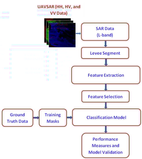
Figure 1.
Block diagram of UAVSAR image processing chain.
In this research, pixel-based polarimetric and window-based texture features were extracted from the SAR data. The pixel-based polarimetric decomposition features such as entropy, anisotropy, scattering angle and texture features from gray level co-occurrence matrix and discrete wavelet transform were computed and analyzed for efficient levee classification.
2.1. Texture Features
It is our hypothesis that both texture-based features and polarimetric features would be useful in analyzing levees for damage. A damaged section of the levee will have structural differences internally, and the surface will also have differences with the surrounding soil. Furthermore, over time, the vegetation around the damaged area may also change due to the moisture coming through the levee. It is anticipated that these changes will be “visible” in features extracted from SAR imagery.
Feature extraction in this study is based on three different feature types, explained in the sections below. GLCM-based features are textural features based on pixel value co-occurrences. Discrete Wavelet Transform-based features are based on a 2D Discrete Wavelet Transform (DWT) analysis. Finally, polarimetric features are based on data derived from the multiple polarization scattering matrix.
In the sequel, Section 2.1.1 discusses the DWT-based features. Section 2.1.2 discusses the GLCM-based features, while Section 2.1.3 discusses the polarimetric features.
2.1.1. DWT-Based Features
The first type of texture features used in this study are based on the DWT. The DWT was first proposed for texture analysis by Mallat [21]. The DWT allows a signal to be decomposed using a series of elemental functions called wavelets, which are based on translations and scaling of the so-called mother wavelet. The mother wavelet for a given scale s and translation u are given by
The wavelet decomposition of a function for a given scale and translation is given by
In practice, dyadic (sizes are powers of two) wavelets can be implemented as a series of high-pass (detail) and low-pass (approximation) filters. When applied to 2D imagery, wavelets decompose the image into different sub-bands. Common features extracted include wavelet decomposition values, absolute values, or energies. The 2D DWT is essentially a double 1D analysis of a 2D signal, by operating on the rows and columns of an image. As shown in Figure 2, the 2D DWT is accomplished by passing the input image through a high-pass filter, g[n], and a low-pass filter, h[n]. The first step applies the filter to the image rows, and the second step applies the filters to the columns. After the filtering, a decimation by two prepares the signal for the next level of decomposition.
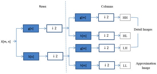
Figure 2.
Schematic diagram of one-level two-dimensional DWT image decomposition process.
A total of 48 DWT coefficients were generated from the analysis using an window. These features were then normalized to the range using the minimum and maximum of each feature. The same data transformations were used with both training and testing data. The low-pass features provide information on the more slowly-varying parts of the signal, e.g., coarse textural information. The high-pass feature provide detail (higher frequency) information. In our analysis, dyadic wavelets were utilized, and window sizes of pixels, pixels, and pixels were analyzed. In Figure 2, the letters H and L refer to high and low pass portions of the DWT analysis, respectively.
2.1.2. GLCM-Based Features
The second type of features analyzed are the GLCM-based features. GLCM analysis is a second-order statistical tool usually used to characterize texture in imagery. The GLCM features analyze imagery based on the frequency of two gray levels appearing in an image according to a position operator. In effect, it is estimating the joint probability of the two gray levels from a pair of pixels along a given distance and direction. The GLCM features are extracted from four spatial orientations: horizontal, left-diagonal, right-diagonal, and vertical. Each of these directions yields one GLCM matrix. From each matrix, six features are extracted: energy, correlation, variance, homogeneity, entropy, and inertia. The formulas for calculating these features are shown in Table 1.

Table 1.
GLCM Features.
In Table 1, is the graylevel matrix value at the coordinate , , and is the variance.
For each radar polarization channel (HH, HV and VV), 24 GLCM texture features are generated, corresponding to the four directions and six types of texture features. In total, 72 GLCM-based features were extracted from the SAR data. In order to quantify the effects of the analysis block size, the window size was varied by pixels, pixels, pixels, and pixels. GLCM analysis requires a center pixel in the analysis window, so all the window dimensions are odd. After feature extraction, the features were normalized to [0,1], using the min-max method.
2.1.3. Polarimetric-Based Features
The third type of features analyzed are polarimetric-based features. In Polarimetric SAR (PolSAR), the transmitted radio frequency signal is polarized. The receiver is able to concurrently receive multiple polarizations, which can be used to help discriminate different scattering mechanisms. The backscattering signal properties are captured in the scattering matrix, S, which is given by
where the subscripts h and v represent horizontal and vertical polarization, respectively. Note that due to symmetry, (since our radar is monostatic, it is usually the case that reciprocity holds; that is, that the cross-polarization scattering factors are identical. This assumption would not necessarily be the case for a bistatic radar, for which reciprocity does not hold.).
To relate the scattering matrix to the physical properties of the scatterer, the target vector is represented in the 3D Pauli basis [22] as given by
The coherency matrix, T, contains the second order statistical information about the target backscatter response, and is given by
where H represents the Hermitian operator (matrix transpose and complex conjugation). For single-look and multi-look processed data, the coherency matrix is defined as:
where the diagonal elements , , give the surface, double-bounce, and volume scattering information about the target, respectively. The VV backscatter dominates at the surface scattering areas, the HV backscatter dominates in the volume scattering, and HH dominates in the double-bounce areas.
Cloude and Pottier [18,22] developed a polarimetric decomposition theorem based on eigenanalysis of the coherency matrix. The decomposition extracts an estimate of the entropy, H, scattering angle , and anisotropy, A, from the coherency matrix [18,22].
The entropy parameter, H, is a measure of the randomness in the backscatter, and is defined as the logarithmic sum of the weighted eigenvalues [23], as given by
where and corresponds to the eigenvalue . For smooth surfaces, H takes on values close to zero, implying a non-depolarizing scattering mechanism. Usually, low entropy indicates a single scattering mechanism, while high entropy indicates more random scattering from multiple point objects.
The anisotropy feature helps to distinguish different types of scattering mechanisms which have different eigenvalue distributions. This parameter examines the second and third eigenvalues and is given by
The anisotropy can be considered a measure of the lack of azimuth symmetry, or as an indication of the small-scale surface roughness. For surfaces with perfect azimuth symmetry, , and the anisotropy is zero. Usually, this feature is a good discriminator when [24]. When the entropy feature is low, the anisotropy is noisy [24]. Since the UAVSAR usually has a good signal-to-noise ratio, the UAVSAR provides good anisotropy values.
The third feature is the mean angle () and is an indicator of the type of scattering mechanism that is occurring. The parameter varies from to and is defined as
where The feature is approximately when the target has a dominant surface or single-bounce component, while indicates volume scattering, and indicates that double-bounce scattering has occurred.
2.2. Support Vector Machine Classifier
The SVM is a nonparametric classification method and has been used successfully in many remote sensing studies. The two-class SVM classifier discriminates two classes by fitting an optimal separating hyperplane to the training data within a kernel-induced feature space. Nonlinear kernel function in the SVM framework helps to map nonlinear separation in the original space to a linear separation in the kernel-induced feature space. Another advantage of SVM is that it often works well with small training data sets. The kernel function plays a critical role in SVM training and classification [25]. The essence of the kernel function is to enable operations to be performed in the input space rather than the high dimensional feature space. Some commonly implemented kernel functions are the linear kernel, polynomial kernel, and the Gaussian radial basis function (RBF) kernel. The RBF is given as
where the parameter is a width parameter that usually must be optimized for the given problem.
3. Materials
The study area is a stretch of 230 km of levees along the lower Mississippi River along the western boundary of the state of Mississippi (MS, USA), as shown in Figure 3. The study area was selected based on the history of levee failure events occurring in the lower Mississippi valley. This history can facilitate the investigation of the use of remote sensing data to analyze physical factors that would indicate problems in levee conditions, whether they arise from moisture content, slope instability, hydraulic uplift, water seepage through levees, or underseepage resulting in sand boils. Figure 4 shows the photograph of Earthen levee on the banks of Albermarle Lake, MS, USA, a Mississippi river oxbow. Levee vegetation consists mostly of grasses and weeds. Three types of grasses predominate on the levees in the study area are: Bermuda, Rye, and Johnsongrass.
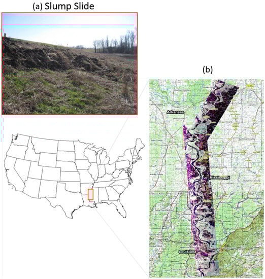
Figure 3.
Map and pictures of study area. (a) Picture of levee slump slide; (b) Study area location.
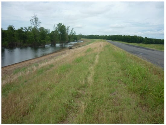
Figure 4.
Earthen Levee on the banks of Albemarle Lake, MS, USA, a Mississippi River oxbow.
The SAR data used in this study were acquired by NASA Jet Propulsion Laboratory’s (JPL) UAVSAR polarimetric L-band ( = 23.98 cm) synthetic aperture radar with a range bandwidth of 80 MHz (resulting in better than 2 m range resolution). UAVSAR is specifically designed to acquire airborne repeat track SAR data for differential interferometric measurements [26]. The single look complex (SLC) data from UAVSAR is of very high resolution with an azimuth slant pixel spacing of 0.6 m and range pixel spacing of 1.6 m. However, the single-look images are very speckled in slant range, which makes visual interpretation and characterization very difficult. To reduce the effects of noise, multi-look cross product (MLC) data is derived from SLC data by averaging a region sized three range pixels by twelve azimuth pixels. These complex cross products preserve most of the important amplitude and phase information that are needed to analyze the data. These products are widely used in radar applications due to speckle reduction by averaging the single-look pixels. The multi-looked SAR data is projected to the ground range using an Earth ellipsoid model and the resultant product is used in this study, which has square pixels of 5.5 m spatial resolution. The instrument is capable of penetrating dry soil to a few centimeters depth, and measuring vertical displacements on the order of a few millimeters. The differences in vegetation growth (sparse or dense) and vegetation type (Bermuda grass, weeds, etc.) influence the radar backscatter and are distinguishable in the imagery. Thus, it is valuable in detecting changes in levees that are key inputs to the classification system.
A multi-polarized radar image acquired in June 2009 has been analyzed in detail for detecting the anomalies on the levees. The UAVSAR flew over the study area for data collection and NASA JPL performed pre-processing of the data by applying radiometric calibrations, geo-registration, and orthorectification. In addition to the radar data, we rely on ground truth data collected by the US Army Corps of Engineers (USACE) and our team in field data collection trips. This data documented the exact location and timing of slough slide appearance, dimensions of the land slides, their repair status, how they were repaired, etc. The USACE maintains a national inventory of levee systems and posts the information on the National Levee Database (NLD) website [27]. It provides information about the location and condition of levees and floodwalls. The ground truth data that is used in this research was obtained from the Engineer Research and Development Center (ERDC) in Vicksburg, Mississippi. This data is tabulated in Table 2. There were three active slide events identified at the time of image acquisition and precise boundaries of the slump slide were mapped with polygons drawn using a GPS instrument during field data collection trips. The ground truth was also compared to the optical NAIP (National Agriculture Imagery Program) data to visually confirm the slide events and training masks were created based on those results. The photograph of an active slump slide shown in Figure 3 (upper left) was taken during one of our field data collection trips. The location of this slide is at the Eagle Lake area near Vicksburg, MS. Training samples of slides and healthy levee areas were obtained from the UAVSAR data using the training masks for feature extraction analysis.
Table 2.
Levee slides’ ground truth data from the Mississippi Levee Board.
The UAVSAR imagery acquired on 16 June 2009 was used in the analysis and the georeferenced layers used in the analyses have been masked by a 40 m buffer from the crown of the levee on the river side. Each pixel of multi-look UAVSAR imagery is 5.5 m × 5.5 m, and the size of the subset is 1.1 km along the levee pixels), which had three reported slide events (Slide number 17, 20 and 21) at the time of image acquisition was used in the analysis. The ground truth data from the Mississippi Levee Board at the time of image acquisition with active slump slides and their repair status along with its dimensions is given in Table 2.
As shown in Figure 5, the levee is divided into two classes, healthy/non-slide levee and slump slide, and the training masks were designed based on the ground truth data. This subset has a total of 102 slump slide pixels and 549 healthy/non-slide levee pixels.
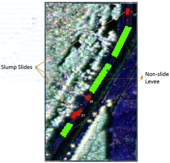
Figure 5.
Training mask for UAVSAR subset with two ground truth classes: slump slide and non-slide/healthy Levee with three-band UAVSAR (HH, HV, and VV) image at the background.
4. Results and Discussion
The SVM was utilized to classify the results for the DWT, GLCM, and Polarimetric features. The SVM can work well even with small training data sets, which is very important for levee applications, as the training data is very small. In this study, the RBF kernel was chosen. The other parameters considered are called hyper parameters and these are the soft margin constant C and the width of the Gaussian kernel . The soft margin constant C controls the penalty of misclassifying training samples.
In this study, the performance of the SVM classifier using three different combinations of groups of features were compared. The texture features from DWT, GLCM and polarimetric features were included separately and the SVM algorithm was implemented using a Gaussian RBF kernel. The performance of the classification was tested with different values of the kernel parameter as well as different window sizes for the texture feature calculations. The regularization parameter C was varied but did not significantly affect the results. Note that the number of training samples is imbalanced: the slump slide class has less pixels than the non-slide levee class and of the labeled samples were used as training and the rest of the pixels were predicted by the classifier. The classification accuracy was also compared by using only the three types of radar polarization channel amplitude data: HH, HV, and VV (without feature sets).
4.1. DWT Feature Results
The SVM algorithm was implemented on the extracted DWT texture features of the SAR data set using a Gaussian RBF kernel and the performance of the classification was tested with different values of the kernel parameter, . The DWT features with different mother wavelets were calculated. However, the Daubechies db-4 mother wavelet [28] gave better accuracies in detecting the slump slides, so only Daubechies wavelet features were analyzed. Figure 6 shows the overall classification accuracies of the SVM classifier with DWT feature set with varying parameter for the RBF kernel and different window size values. Figure 7 shows the wavelet features superimposed on an aerial image. This figure also shows the SVM classification results.
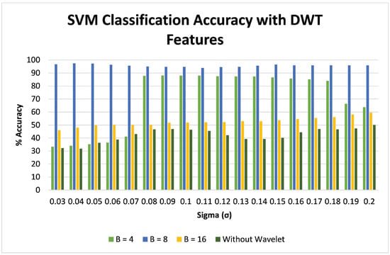
Figure 6.
Classification accuracy (%) of SVM classifier with DWT features with different block/window sizes (window is pixels).
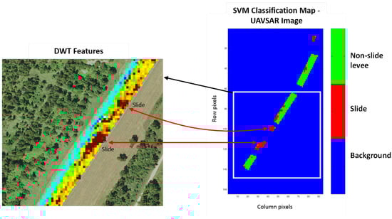
Figure 7.
SVM Classification. The SVM Classification map for UAVSAR data set using DWT features with and wavelet block size (window is ) is shown on the right. On the left is a enlarged overlay of the wavelet features (with an aerial image background).
From Figure 6, the pixel window size produced the best results, and this window size did not show a significant change as the SVM RBF parameter was varied. The pixel window size produced the highest accuracies of for the slide class and for the non-slide levee class. The and pixel window sizes had significantly poor results. The performance of the classifier was also compared by using only the three types of radar polarization channel data, HH, HV, and VV (without wavelet features), which resulted in lower classification accuracies. The accuracy assessment was conducted ten times (using randomly selected training samples), and the results were averaged. The confusion matrix from one of the ten runs with and wavelet block size is given in Table 3, and the classification map ( and ) is shown in Figure 7.
Table 3.
Confusion matrix of SVM classifier output using the DWT features with and block size pixels.
4.2. GLCM Feature Results
The GLCM features energy, correlation, variance, homogeneity, entropy, and inertia were computed and the SVM classifier was trained and tested with this extracted feature data. The classification was performed with different block size windows: pixels, pixels, pixels, and pixels. The results showed that the classifier performed well with GLCM window size pixels having the highest accuracies of and for the slide and non-slide levee class, respectively. The confusion matrix of one of the ten runs of GLCM feature classification with and window size pixels is shown in Table 4. The classification accuracies with different values and window sizes is shown in Figure 8. In general, the pixels had the worst performance, the pixels had slightly better performance, the pixels even better performance, and pixels the best performance. This is somewhat similar to what was seen in the DWT-based features, where the best window size was pixels. A window that is too small will have more inaccurate mean and variance estimates, and a window that is too large can include pixels that cross slide boundaries, providing a mixed evaluation that includes features from slide pixels as well as non-slide pixels. This analysis shows that one must try various window sizes in order to determine the best results. Figure 9 shows the classification map for the GLCM results.
Table 4.
Confusion matrix of SVM classifier output with GLCM features, , and block size .
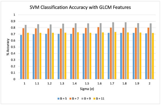
Figure 8.
Classification accuracy (%) of SVM classifier with GLCM features with different block/window size (window is pixels).
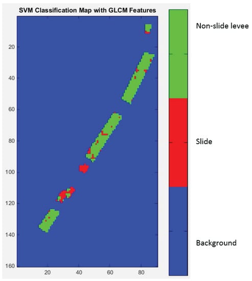
Figure 9.
SVM Classification map for UAVSAR data set using GLCM features with and block size (window is ).
4.3. Polarimetric Feature Results
From the radar polarimetric backscatter data, the coherency matrix was computed, which contains the second order statistical information about the polarization. The decomposition parameters entropy (H), anisotropy (A) and scattering angle () were derived from the eigenvalue decomposition of the coherency matrix.
4.3.1. Entropy
The parameter entropy (H) indicates the degree of randomness of the scattering medium. The slump slides are usually rough in texture, which will result high entropy values. However, the levees in our study area are covered with vegetation (different types of grass—mostly Bermuda, Rye, Johnson grass and weeds in some areas), so the river side of the levee has moderate to high entropy values. From the entropy map shown in Figure 10a, it is clear that the slump slides have high entropy values ranging from 0.48 to 0.72.
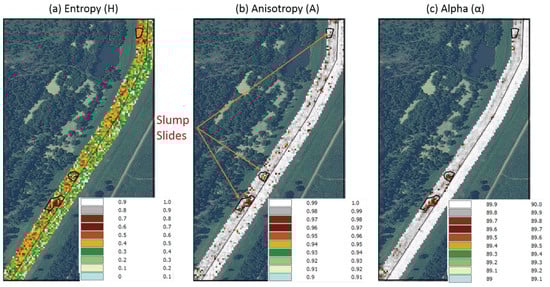
Figure 10.
Polarimetric features from 16 June 2009 UAVSAR subset with optical NAIP imagery background. The slump slides are shown by the small black polygons in the images. (a) entropy (ranges from 0 to 1); (b) anisotropy (ranges from 0 to 1); (c) scattering angle (ranges from to ).
4.3.2. Anisotrophy
In general, the anisotropy values will be affected by the size and type of vegetation, the time of year (season), and by how much of the radar signal is reflected by the ground vegetation versus how much is reflecting from the ground. The UAVSAR’s L-Band instrument has a relatively long wavelength, so it penetrates through short vegetation and the backscatter is mostly from the underlying ground. However, the vegetation in the study area is about 2–3 feet high at the time of image acquisition (June 2009), so double bounce scattering dominates and the values of entropy and anisotropy are relatively high. However, the slump slide areas, as shown in Figure 3, are without vegetation and are relatively rough in texture, so the anisotropy values are comparatively lower than the surrounding non-slide areas of the levee. The values of anisotropy within the slump slide areas range from 0.95 to 0.98 (Figure 10b).
4.3.3. Scattering Angle
The angle corresponds to the variation in scattering mechanism, with corresponding to surface scattering; , dipole scattering; and , double bounce scattering. For smooth surfaces, surface scattering dominates and the entropy is close to 0. As shown in Figure 10c, the alpha values are very high due to double-bounce scattering. The slump slides are rough in texture with certain depth, so these areas resulted in double-bounce scattering. In addition, the vegetation on the levee also causes double-bounce scattering, resulting in high values of scattering angles all through the levee. The alpha values within the slump slide range from to .
4.3.4. SVM Classification Results
The support vector machine algorithm was implemented based on the polarimetric target decomposition parameters entropy, anisotropy, and scattering angle derived from the eigenvalue decomposition of the coherency matrix. The UAVSAR subset of Figure 5 was used and the classifier was trained with of the labeled data. The classifier accuracies were and for slump slide and non-slide/healthy levee, achieved at as shown in Figure 11.
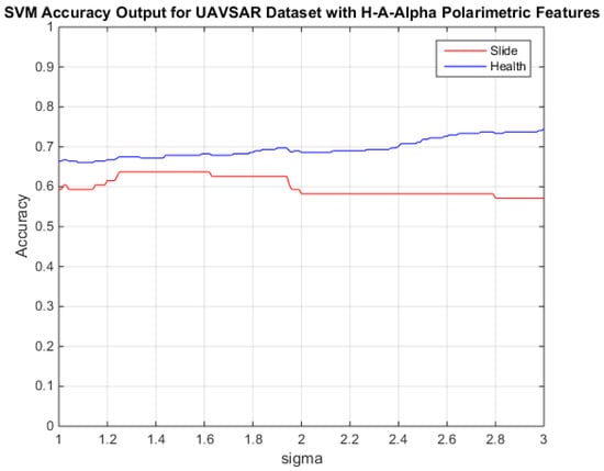
Figure 11.
SVM classifier accuracies with polarimetric decomposition feature set (H, A, and ) for UAVSAR subset of 16 June 2009 versus . The blue line is healthy levee and the red line slump slides.
5. Conclusions and Future Work
In this paper, DWT, GLCM and polarimetric-based features from SAR data were used with a SVM classifier to detect slump slides on levees. The DWT features performed the best, having an overall accuracy of with a window size of pixels across a wide range of RBF parameters. The window size had a large effect on the overall accuracy with the DWT-based features. The GLCM features also performed well, with an overall accuracy of . These features were also sensitive to the window size. The polarimetric-based features had the lowest performance, but the anisotropy and scattering angle parameters did provide some discriminative values for detecting slump slides.
The levee area is segmented based on the orientation of the levee in the SAR image. That is, we wanted the select regions of the levee where the levee was basically oriented in one direction, versus areas where the levee made sharp changes to follow the river. The reason was that the backscatter will appear differently if the levee changes direction sharply. The segments are created based on human ground truth data on existing slide events at the time of the image acquisition. There were only a small amount of training and testing pixels available, and the SVM did a good job with the limited data.
In the future, we plan to perform several more experiments. First, X-band satellite data is also available, and it could be used and compared to the current L-band data. Furthermore, data fusion between these two radars could be performed, as each could provide different information about the levee health. In addition, feature-level fusion could be performed across the different features used in this study. Decision-level fusion can be applied by using multiple SVMs and fusing the results. Multiple Kernel Learning (MKL) [29,30] can also be applied, which searches for an optimal linear combination of kernels which are utilized in multiple SVMs.
Deep learning has made significant progress in analyzing optical, LiDAR [31], and SAR [32,33,34,35,36] data. Extending these architectures (or modifying them) for SAR data processing promises even better results. The challenge here is the small amount of training data. The benefit (other than high classification accuracies) is that the deep learning network can learn the features from the data, versus hand-coded features (e.g., the features we used in this paper). We also want to examine levee segmentation by an automated algorithm (probably requiring GPS data or other Graphical Information System data). This could also be a good task for a deep learning system.
Finally, we want to examine computing the GLCM features on PolSAR decomposition features, e.g., Yamaguchi decomposition [37] features, which would effectively combine PolSAR radar returns and SAR textural features.
Acknowledgments
This material is based upon work supported by the National Science Foundation under Award No. OISE-1243539, and by the National Aeronautics and Space Administration (NASA, Pasadena, CA, USA) Applied Sciences Division. The authors would like to thank the US Army Corps of Engineers, Engineer Research and Development Center and Vicksburg Levee District (Vicksburg, MS, USA) for providing ground truth data and expertise, and also NASA Jet Propulsion Laboratory (JPL) for providing the UAVSAR image and initial data processing. We also acknowledge the anonymous reviewers who provided excellent suggestions for improving the paper.
Author Contributions
L.D. and J.V.A. conceived and designed the experiments; L.D. performed the experiments; L.D., J.V.A., J.E.B. and N.H.Y. analyzed the data; L.D., J.V.A., and J.E.B. and N.H.Y. wrote the paper.
Conflicts of Interest
The authors declare no conflict of interest.
Abbreviations
The following abbreviations are used in this manuscript:
| DWT | Discrete Wavelet Transform |
| GLCM | Gray Level Co-Occurrence Matrix |
| GPS | Global Positioning System |
| JPL | Jet Propulsion Laboratory |
| MLC | Multi Look Cross product |
| NASA | National Aeronautics and Space Administration |
| NAIP | National Agriculture Imagery Program |
| PolSAR | Polarimetric SAR |
| RBF | Radial Basis Function |
| RX | Reed-Xiaoli |
| SAR | Synthetic Aperture Imagery |
| SLC | Single Look Complex |
| STC | Silverman–Totman–Caefer |
| UAVSAR | Uninhabited Aerial Vehicle Synthetic Aperture Radar |
| USACE | US Army Corps of Engineers |
References
- Rogers, D. Evolution of the Levee System along the Lower Mississippi River; University of Missouri-Rolla: Rolla, MO, USA, 2005. [Google Scholar]
- Lascano, R.J.; Baumhardt, R.L.; Hicks, S.K.; Landivar, J.A. Spatial and temporal distribution of surface water content in a large agricultural field. Precis. Agric. 1999, precisionagric4a, 19–30. [Google Scholar]
- Jones, C.E.; Bawden, G.; Deverel, S.; Dudas, J.; Hensley, S.; Yun, S.H. Study of movement and seepage along levees using DINSAR and the airborne UAVSAR instrument. In Proceedings of the SPIE Remote Sensing, International Society for Optics and Photonics, Edinburgh, Scotland, 9–12 December 2012; p. 85360E. [Google Scholar] [CrossRef]
- Dabbiru, L.; Aanstoos, J.V.; Younan, N.H. Earthen levee slide detection via automated analysis of synthetic aperture radar imagery. Landslides 2016, 13, 643–652. [Google Scholar] [CrossRef]
- Cundill, S.L.; van der Meijde, M.; Hack, H.R.G. Investigation of remote sensing for potential use in dike inspection. IEEE J. Sel. Top. Appl. Earth Obs. Remote Sens. 2014, 7, 733–746. [Google Scholar] [CrossRef]
- Rignot, E.; Chellappa, R.; Dubois, P. Unsupervised segmentation of polarimetric SAR data using the covariance matrix. IEEE Trans. Geosci. Remote Sens. 1992, 30, 697–705. [Google Scholar] [CrossRef]
- Fukuda, S.; Hirosawa, H. Support vector machine classification of land cover: Application to polarimetric SAR data. In Proceedings of the IEEE 2001 International Geoscience and Remote Sensing Symposium (IGARSS’01), Syndey, Austrlia, 9–13 July 2001; IEEE: Piscataway, NJ, USA, 2001; Volume 1, pp. 187–189. [Google Scholar]
- Waske, B.; Benediktsson, J.A. Fusion of support vector machines for classification of multisensor data. IEEE Trans. Geosci. Remote Sens. 2007, 45, 3858–3866. [Google Scholar] [CrossRef]
- Zhang, L.; Zou, B.; Zhang, J.; Zhang, Y. Classification of polarimetric SAR image based on support vector machine using multiple-component scattering model and texture features. EURASIP J. Adv. Signal Process. 2009, 2010, 1. [Google Scholar] [CrossRef]
- Haralick, R.M.; Shanmugam, K. Textural features for image classification. IEEE Trans. Syst. Man Cybern. 1973, 3, 610–621. [Google Scholar] [CrossRef]
- Anys, H.; He, D.C. Evaluation of textural and multipolarization radar features for crop classification. IEEE Trans. Geosci. Remote Sens. 1995, 33, 1170–1181. [Google Scholar] [CrossRef]
- Cui, M.; Prasad, S.; Mahrooghy, M.; Aanstoos, J.V.; Lee, M.A.; Bruce, L.M. Decision fusion of textural features derived from polarimetric data for levee assessment. IEEE J. Sel. Top. Appl. Earth Obs. Remote Sens. 2012, 5, 970–976. [Google Scholar] [CrossRef]
- Soh, L.K.; Tsatsoulis, C. Texture analysis of SAR sea ice imagery using gray level co-occurrence matrices. IEEE Trans. Geosci. Remote Sens. 1999, 37, 780–795. [Google Scholar] [CrossRef]
- Hossain, A.A.; Easson, G.; Hasan, K. Detection of levee slides using commercially available remotely sensed data. Environ. Eng. Geosci. 2006, 12, 235–246. [Google Scholar] [CrossRef]
- Dabbiru, L.; Aanstoos, J.V.; Younan, N.H. Classification of levees using polarimetric synthetic aperture radar (SAR) imagery. In Proceedings of the 2010 IEEE 39th Applied Imagery Pattern Recognition Workshop (AIPR), Washington, DC, USA, 13–15 October 2010; IEEE: Piscataway, NJ, USA, 2010; pp. 1–5. [Google Scholar]
- Melamed, G.; Rotman, S.R.; Blumberg, D.G.; Weiss, A.J. Anomaly detection in multi-polarimetric radar images. In Proceedings of the IEEE 25th Convention of Electrical and Electronics Engineers in Israel (IEEEI 2008), Eilat, Israel, 3–5 December 2008; IEEE: Piscataway, NJ, USA, 2008; pp. 558–562. [Google Scholar]
- Pottier, E.; Lee, J.S.; Ferro-Famil, L. Advanced Concepts in Polarimetric SAR Image Analysis—A Tutorial Review. Available online: https://pdfs.semanticscholar.org/60d3/eb04964daf184b931ded10796bcb0b54e69f.pdf (accessed on 31 April 2017).
- Cloude, S.R.; Pottier, E. A review of target decomposition theorems in radar polarimetry. IEEE Trans. Geosci. Remote Sens. 1996, 34, 498–518. [Google Scholar] [CrossRef]
- Aanstoos, J.V.; Hasan, K.; O’Hara, C.; Prasad, S.; Dabbiru, L.; Mahrooghy, M.; Nobrega, R.; Lee, M.; Shrestha, B. Use of remote sensing to screen earthen levees. In Proceedings of the 2010 39th IEEE Applied Imagery Pattern Recognition Workshop, Washington, DC, USA, 13–15 October 2010; IEEE: Washington, DC, USA, 2010. [Google Scholar]
- Dabbiru, L.; Aanstoos, J.V.; Mahrooghy, M.; Li, W.; Shanker, A.; Younan, N.H. Levee anomaly detection using polarimetric synthetic aperture radar data. In Proceedings of the 2012 IEEE International Geoscience and Remote Sensing Symposium, Munich, Germany, 22–27 July 2012; IEEE: Piscataway, NJ, USA, 2012; pp. 5113–5116. [Google Scholar]
- Mallat, S.G. A theory for multiresolution signal decomposition: The wavelet representation. IEEE Trans. Pattern Anal. Mach. Intell. 1989, 11, 674–693. [Google Scholar] [CrossRef]
- Cloude, S.R.; Pottier, E. An entropy based classification scheme for land applications of polarimetric SAR. IEEE Trans. Geosci. Remote Sens. 1997, 35, 68–78. [Google Scholar] [CrossRef]
- Polarsar Pro Manual, Singlue vs. Multi-Polarization Descriptors. Available online: http://earth.eo.esa.int/polsarpro/Manuals/3_Single_vs_multi-polarization_descriptors.pdf (accessed on 5 December 2016).
- Lee, J.S.; Pottier, E. Polarimetric Radar Imaging: From Basics to Applications; CRC Press: Boca Raton, FL, USA, 2009. [Google Scholar]
- Burges, C.J. A tutorial on support vector machines for pattern recognition. Data Min. Knowl. Discov. 1998, 2, 121–167. [Google Scholar] [CrossRef]
- Rosen, P.A.; Hensley, S.; Wheeler, K.; Sadowy, G.; Miller, T.; Shaffer, S.; Muellerschoen, R.; Jones, C.; Zebker, H.; Madsen, S. UAVSAR: A new NASA airborne SAR system for science and technology research. In Proceedings of the 2006 IEEE Conference on Radar, Verona, NY, USA, 24–27 April 2006; IEEE: Piscataway, NJ, USA, 2006; pp. 22–29. [Google Scholar]
- US Army Corps of Engineers. National Levee Database (NLD). Available online: http://www.usace.army.mil/Missions/CivilWorks/LeveeSafetyProgram/NationalLeveeDatabase.aspx (accessed on 15 March 2017).
- Daubechies, I. Ten Lectures on Wavelets; SIAM: Philadelphia, PA, USA, 1992; Volume 61. [Google Scholar]
- Du, X.; Zare, A.; Keller, J.M.; Anderson, D.T. Multiple Instance Choquet integral for classifier fusion. In Proceedings of the 2016 IEEE Congress on Evolutionary Computation (CEC), Vancouver, BC, Canada, 24–29 July 2016; pp. 1054–1061. [Google Scholar]
- Pinar, A.J.; Rice, J.; Hu, L.; Anderson, D.T.; Havens, T.C. Efficient Multiple Kernel Classification using Feature and Decision Level Fusion. IEEE Trans. Fuzzy Syst. 2016. [Google Scholar] [CrossRef]
- Maturana, D.; Scherer, S. VoxNet: A 3D Convolutional Neural Network for Real-Time Object Recognition. In Proceedings of the 2015 IEEE/RSJ International Conference on Intelligent Robots and Systems (IROS), Hamburg, Germany, 28 September–2 October 2015; pp. 922–928. [Google Scholar]
- Geng, J.; Fan, J.; Wang, H.; Ma, X.; Li, B.; Chen, F. High-Resolution SAR Image Classification via Deep Convolutional Autoencoders. IEEE Geosci. Remote Sens. Lett. 2015, 12, 2351–2355. [Google Scholar] [CrossRef]
- Benediktsson, J.A.; Chanussot, J.; Moon, W.W. Very High-Resolution Remote Sensing: Challenges and Opportunities. Proc. IEEE 2012, 100, 1907–1910. [Google Scholar] [CrossRef]
- Hou, B.; Luo, X.; Wang, S.; Jiao, L.; Zhang, X. Polarimetric SAR images classification using deep belief networks with learning features. In Proceedings of the 2015 IEEE International Geoscience and Remote Sensing Symposium (IGARSS), Milan, Italy, 26–31 July 2015; IEEE: Piscataway, NJ, USA, 2015; pp. 2366–2369. [Google Scholar]
- Liu, H.; Min, Q.; Sun, C.; Zhao, J.; Yang, S.; Hou, B.; Feng, J.; Jiao, L. Terrain classification with Polarimetric SAR based on Deep Sparse Filtering Network. In Proceedings of the 2016 IEEE International Geoscience and Remote Sensing Symposium (IGARSS), Beijing, China, 10–15 July 2016; IEEE: Piscataway, NJ, USA, 2016; pp. 64–67. [Google Scholar]
- Tanase, R.; Datcu, M.; Raducanu, D. A convolutional deep belief network for polarimetric SAR data feature extraction. In Proceedings of the 2016 IEEE InternationalGeoscience and Remote Sensing Symposium (IGARSS), Beijing, China, 10–15 July 2016; IEEE: Piscataway, NJ, USA, 2016; pp. 7545–7548. [Google Scholar]
- Yamaguchi, Y.; Moriyama, T.; Ishido, M.; Yamada, H. Four-component scattering model for polarimetric SAR image decomposition. IEEE Trans. Geosci. Remote Sens. 2005, 43, 1699–1706. [Google Scholar] [CrossRef]
© 2017 by the authors. Licensee MDPI, Basel, Switzerland. This article is an open access article distributed under the terms and conditions of the Creative Commons Attribution (CC BY) license (http://creativecommons.org/licenses/by/4.0/).