1. Introduction
In recent years we have witnesed an unprecedented growth in internet traffic due to the advent of new applications which are based on high performance computing (HPC) and cloud computing infrastructure in data centers. Social networks, multimedia gaming and streaming applications, website searching, scientific calculations/computations and distributed services are some examples of bandwidth-hungry applications, and their bandwidth demand is increasing exponentially. Today’s data centers comprise thousands of servers with high speed links and are interconnected via switches and routers. As the size and complexity of data center deployments increase, meeting their high bandwidth requirements is a challenge.
Optical networks for data centers have gained significant attention over the last few years due to the potential and benefits of using optical components. The microelectromechanical system (MEMS) optical cross connect (OXC) or OCS switch has been used in the backbone optical network for many years. The attractions of MEMS switches include: (a) excellent power efficiency due to the use of passive switching; (b) high port density; (c) low insertion loss and crosstalk; (d) absence of transceivers due to using all optical switching; (e) lower cost; (f) support of bidirectional communication; and (g) data rate independence. They are also highly scalable and are commercially available e.g., 3D-MEMS [
1]. Hybrid designs for data center networks that use OCS in conjunction with other technologies have been proposed [
2,
3,
4,
5,
6,
7]. Helios and cThrough [
2,
3] propose using OCS in conjunction with traditional electrical packet switching (EPS) while the LIGHTNESS project [
4,
5] employs OCS together with optical packet switching (OPS). The Hydra and OSA [
6,
7] augment OCS with a multi-hopping technique. A major issue with these interconnects has been their slow reconfiguration time due to the limitation of 3D-MEMS technology. This reconfiguration time is influenced by two factors: (1) the switching time of the 3D-MEMS switch,
i.e., 10–100 ms, and (2) the software/control plane overhead required for the estimation of traffic demand and the calculation of a new OCS topology,
i.e., 100 ms to 1 s. Consequently, the control plane can only support applications that have high traffic stability,
i.e., workloads that last several seconds [
2].
Fast optical switching technologies have become available that improve upon the 3D-MEMS OCS switch [
8,
9,
10,
11,
12]. These switches can be built using technologies such as arrayed waveguide grating routers (AWGRs), semiconductor optical amplifiers (SOAs), 1 ×
N photonic switches and wavelength selective switches (WSSs). An AWGR switch is a wavelength router that works in conjunction with tunable wavelength converters (TWCs) or tunable lasers (TLs). An SOA is an amplifier that also works as a gate switch. It provides ON/OFF switching. Photonic switches with 1 ×
N configurations are available and they can be used in the Spanke architecture [
13] to enable a large switching fabric. AWGR, SOA and photonic switches have switching times in the range of a few nanoseconds, much faster than the 3D-MEMS switch’s tens of milliseconds. WSSs divide an incoming set of wavelengths to a different set of outgoing wavelengths. The switching time of WSSs is few microseconds [
11].
In this paper, we evaluate the performance of an enhanced OCS, suitable for use in HPC and in data center networks, that makes use of the faster switching technologies that are now available. We use network-level simulation of short-lived circuits to demonstrate its performance in demanding traffic scenarios. The modelled switch architecture features fast optical switches in a single hop topology with a centralized software-defined optical control plane that uses control packets. The round trip time (RTT) of control packets is high if used in the backbone optical network or in data centers using 3D MEMS. The RTT in our design is lower for several reasons: (1) the propagation delay is negligible; (2) faster optical switches are used at the core; (3) a fast optical control plane is used; (4) processing of the control packet is rapid and (5) a single hop topology is used [
14]. Operational parameters of our system, specifically the traffic aggregation time, can be tuned to better accommodate circuits of various durations and we investigate the effect of such tuning on OCS performance with various workloads. Our results show that, with suitable choices for the OCS system parameters, delay performance comparable to that of an electrical data center network can be achieved.
The remainder of this article is structured as follows.
Section 2 describes the OCS design being modelled. We discuss the scenarios used in performance evaluation in
Section 3 and present the results obtained in
Section 4.
Section 5 contains our conclusions.
2. OCS for Data Center Network
We employ OCS in the proposed data center network architecture. We aggregate packet traffic to create circuits of short duration. A control packet is created to request the allocation of resources needed to establish the circuit from the controller by using a two-way reservation process similar to that proposed for optical burst switching networks [
15]. Although such two-way reservation is not feasible in a longhaul backbone network, in data centers it is suitable for the reasons presented earlier. The controller assigns resources and sends the control packet back to the originating node as an acknowledgement. The data packets in the circuit are then transmitted on the pre-established path configured by the controller.
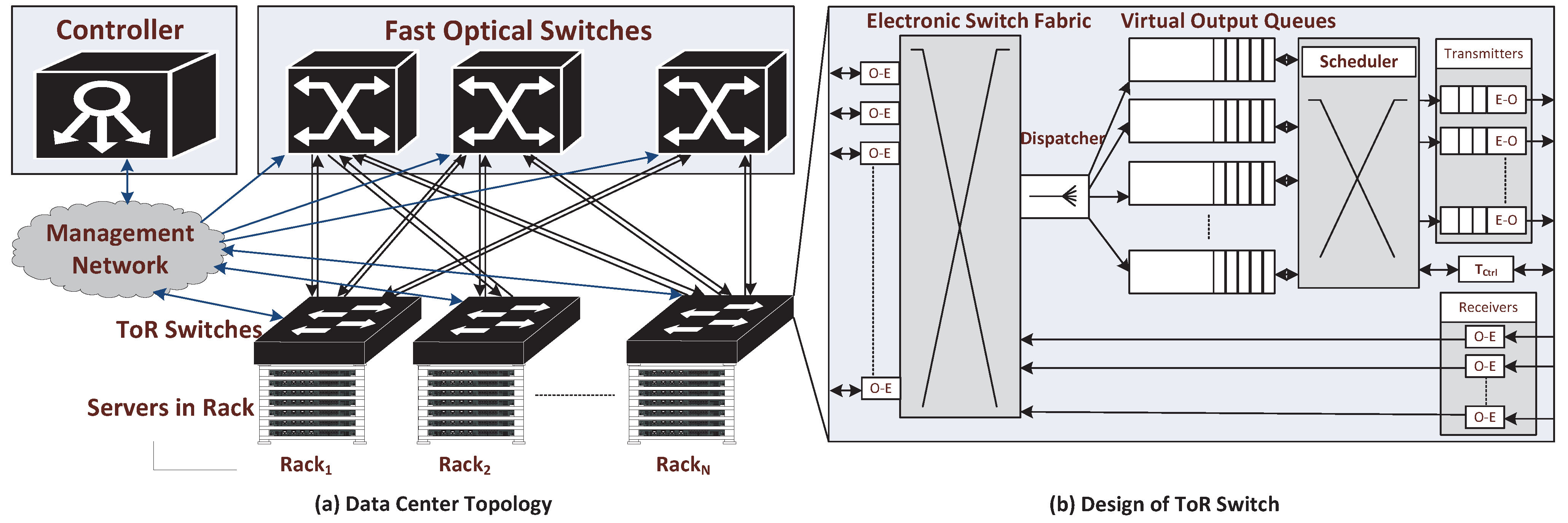
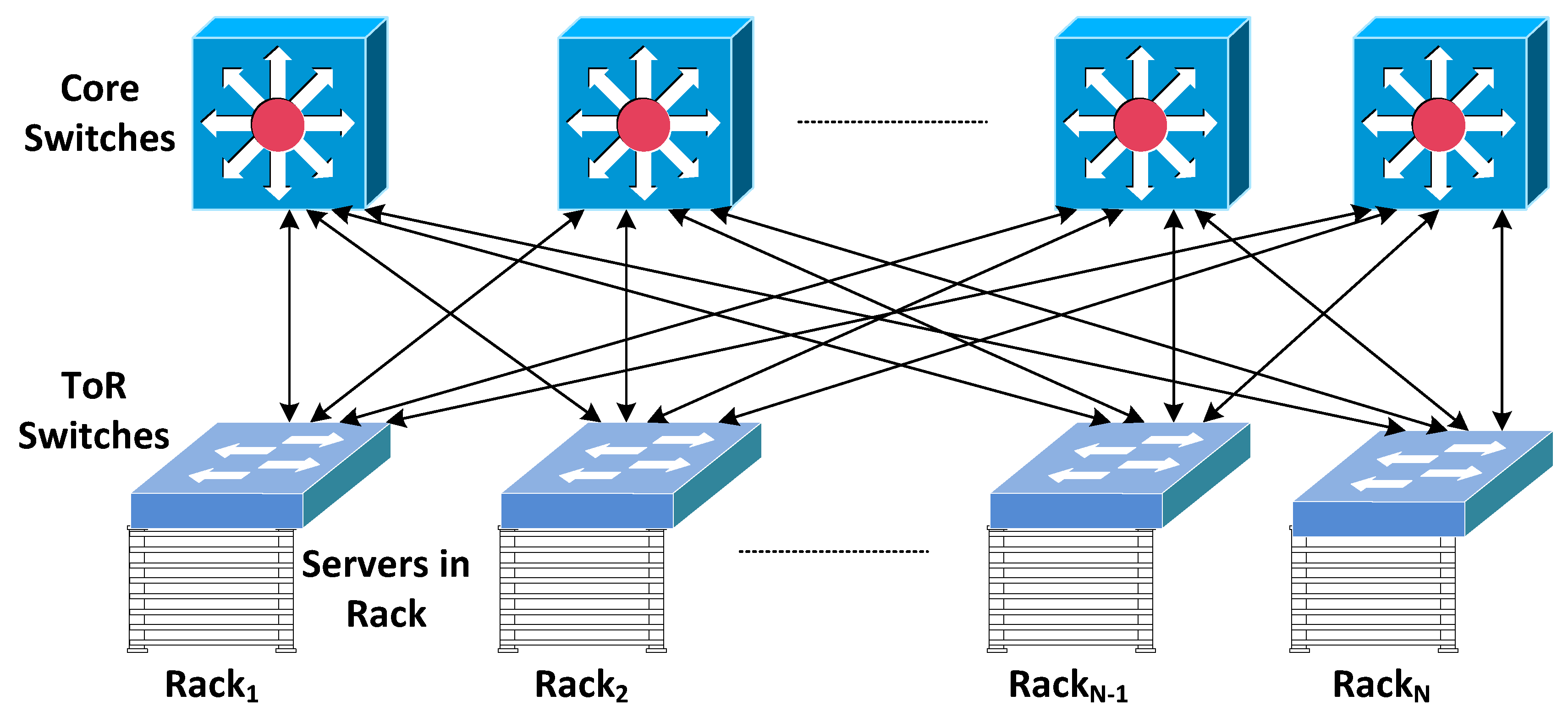
This architecture is shown in
Figure 1a. The proposed topology has two layers,
i.e., edge and core. The edge contains electronic Top of the Rack (ToR) switches while the core comprises a group of fast optical switches. Servers in each rack are connected to the ToR switches using bidirectional optical fibers. The ToR switches are linked to the optical switches using unidirectional optical fibers.
Figure 1.
(a) Topology Diagram for Data Center Network and (b) Design of ToR switches.
Figure 1.
(a) Topology Diagram for Data Center Network and (b) Design of ToR switches.
The proposed design features separate control and data planes. The control plane comprises a centralized controller. The controller performs routing, scheduling and switch configuration functions. It receives connection setup requests from all ToR switches, finds routes, assigns timeslots to the connection requests, and configures optical switches with respect to the timeslots allocated. In order to perform these tasks, the controller keeps a record of the connection states of all optical switches. The data plane comprises optical switches that perform data forwarding on pre-configured lightpaths set up by the controller. A management network is used by the control plane that connects every ToR switch to the controller via a transceiver in each ToR switch reserved for use by control plane. Further details of this architecture are given elsewhere [
16].
2.1. ToR Switch Design
The design of the ToR switch is shown in
Figure 1b. The ToR switch performs intra-rack (same rack) switching using an electronic switch fabric. In order to route traffic to different racks (inter-rack), we consider (
N − 1) virtual output queues (VOQs) where
N represents the total number of ToR switches in the network. Most modern ToR switches support hundreds of VOQs. One VOQ is required for each destination rack. Packets going to the same destination rack are aggregated into the same VOQ. The VOQ not only aggregates traffic but it also avoids head of line blocking (HOL). The dispatcher module of the ToR switch sends each packet to the required VOQ by extracting network address from the destination IP address of the packet and matching it with the VOQ network address.
After traffic aggregation in the VOQ, a control packet is created to request a timeslot from the controller. The timeslot duration corresponds to the duration of the circuit,
i.e., the transmission time for the number of bits aggregated into the circuit by the VOQ. The controller processes the control packet to assign an optical path and a timeslot on that path to the circuit. The requesting VOQ is advised of this path by being told the relevant output port number of the corresponding ToR switch. The control packet is updated with this information and is returned to the ToR switch. The allocation process is described in
Section 2.2. The data transmission proceeds via the assigned port number immediately after the control packet arrives back at the ToR switch. If the timeslot is not immediately available, the controller holds onto the control packet until it is.
We consider a timer-based algorithm for traffic aggregation which is shown in Algorithm 1. The timer starts when a packet reaches the empty VOQ (lines 8–11 in Algorithm 1). If the VOQ is not empty when the packet arrives, it joins other packets in the VOQ (lines 13–14 in Algorithm 1). Upon expiration of the timer, the control packet is created and is sent to the controller to request a new timeslot (lines 3–7 in Algorithm 1). At this stage, the control packet comprises the requested circuit length in bytes and the IP addresses of source and destination ToR switches. The controller performs routing and scheduling algorithm as described in
Section 2.2, assigns a timeslot in the optical switch path and allocates ToR port number to which circuit is to be transmitted and sends it back to the ToR switch.
The control packet now contains the ToR port number assigned by the controller and the circuit length. The scheduler in the ToR switch sends packets according to the circuit length to the queue of the assigned port. This procedure is called circuit transmission and is shown in Algorithm 2. A number of packets corresponding to the circuit length are extracted from the VOQ and are sent to the assigned port for transmission (lines 5–9 in Algorithm 2). The scheduler also starts a new timer if the VOQ is not empty after circuit transmission because new packets might have arrived during the RTT of the control packet (lines 14–22 in Algorithm 2).
| Algorithm 1 Traffic Aggregation Mechanism at ToR Switch |
| Require: timeout ← timeout Parameter |
| {timeout parameter is required during ToR switches configuration} |
| 1: | timeoutevent ← NULL |
| 2: | circuit_length ← 0 {Initialize parameters.} |
| 3: | if timeoutevent then |
| 4: | control_packet ← generateControlPacket() |
| 5: | control_packet.setCircuitLength(circuit_length) |
| 6: | send(control_packet, Tctrl) |
| {timeoutevent is for timer check. This block is executed when timeoutevent occurs, i.e., when timer expires. The control packet is generated and is sent to the management network} |
| 7: | else |
| 8: | pk ← packet arrives |
| 9: | if VOQ.empty() then |
| 10: | firstpk_time ← current_time |
| 11: | schedule(firstpk_time + timeout, timeoutevent) |
| {Schedule timeoutevent by adding timeout parameter in first packet’s arrival time} |
| 12: | end if |
| 13: | circuit_length+ = pk.length |
| 14: | VOQ.insert Packet(pk) |
| {Add packet in virtual output queue} |
| 15: | end if |
2.2. Routing and Scheduling
The controller keeps a record of the connections of all optical switches. It performs routing, scheduling and optical switch configuration. The routing and scheduling mechanism is depicted in Algorithm 3. The controller first gets the source and destination IP addresses from the incoming control packet and reads the source and destination IDs of the ToR switches (lines 2–3 in Algorithm 3). We employ a horizon-based scheduling algorithm similar to that presented for optical burst switching networks [
15]. The term horizon is defined as the latest available time when the channel will be free. By using horizon scheduling, the controller finds source and destination ports of optical switches and their horizons (lines 4–6 in Algorithm 3). The next step is to create a timeslot on the basis of the requested circuit length and to set up a path for this circuit (lines 9–12 in Algorithm 3). After setting up the path in the horizon table, the controller sets the port number of the ToR switch to which circuit will be assigned (line 12 in Algorithm 3). Finally, it sends the control packet back to the ToR switch when the circuit transmission time is about to start (line 13 in Algorithm 3).
Switch configuration is the final task of the controller. After processing the control packet, a configuration message is generated and is sent to the switch controller for optical switch configuration. The switch controller configures the optical switch according to the instructions in the configuration message. The switch controller can control multiple optical switches.
| Algorithm 2 Circuit Transmission at ToR Switch |
| Require: timeout ← timeout Parameter |
| 1: | cp ← control packet arrives |
| 2: | circuitsize ← cp.getSize() |
| 3: | portno ← cp.getPortNo() |
| {Initialization of different variables when the control packet arrives at the ToR switch after being processed by the controller.} |
| 4: | length ← 0 |
| 5: | while VOQ.hasPackets() do |
| 6: | if length ≤ circuitsize then |
| 7: | packet ← VOQ.getPacket() |
| 8: | length+ = packet.length |
| 9: | send(packet, portno) |
| 10: | else |
| 11: | break |
| 12: | end if |
| 13: | end while |
| {Following steps reinitialize variables after circuit transmission.} |
| 14: | if VOQ → empty() then |
| 15: | circuit_length ← 0 |
| 16: | firstpk_time ← 0 |
| 17: | else |
| 18: | pk ← VOQ.get(0) |
| 19: | firstpk_time ← pk.arrivaltime |
| 20: | schedule(firstpk_time + timeout, timeoutevent) |
| 21: | circuit_length ← VOQ.getTotalPacketsLength() |
| 22: | end if |
| Algorithm 3 Routing and Scheduling |
| 1: | cp ← control packet arrives at the controller |
| 2: | sID ← getSrcId(cp.getSourceToRAddress) |
| 3: | dID ← getDestId((cp.getDestToRAddress) |
| {Above lines get source and destination IDs of ToR switches} |
| 4: | src_ch ← getH_Ch(sID) |
| 5: | dest_ch ← getH_Ch(dID) |
| {Above methods return channels of latest horizon} |
| 6: | Tfast ← getMax(getH(src_ch), getH(dest_ch)) |
| {Above methods return latest horizon} |
| 7: | CL ← cp.getCircuitLength() |
| 8: | TRL ← CL ∗ 8/Datarate |
| {Requested timeslot TRL is calculated from circuit length (CL) in the control packet.} |
| 9: | Tstart ← Tfast + Tswf + Tproc + Toverhad |
| 10: | Tend ← Tstart + TRL + Tguard |
| {Above lines represent starting and ending time of timeslot.} |
| 11: | setupPath(src_ch, dest_ch, Tstart, Tend, Tcur) {Horizon is updated} |
| 12: | cp.setchannel(K + (src_ch (mod ch))){Port to port mapping from horizon table to ToR switch} |
| 13: | sendAt(cp, Tstart − Toverhad){Control packet is sent back to the source ToR.} |
2.3. Fast Optical Switches
Recent years have seen the introduction of new types of faster optical switches, some of which are described below.
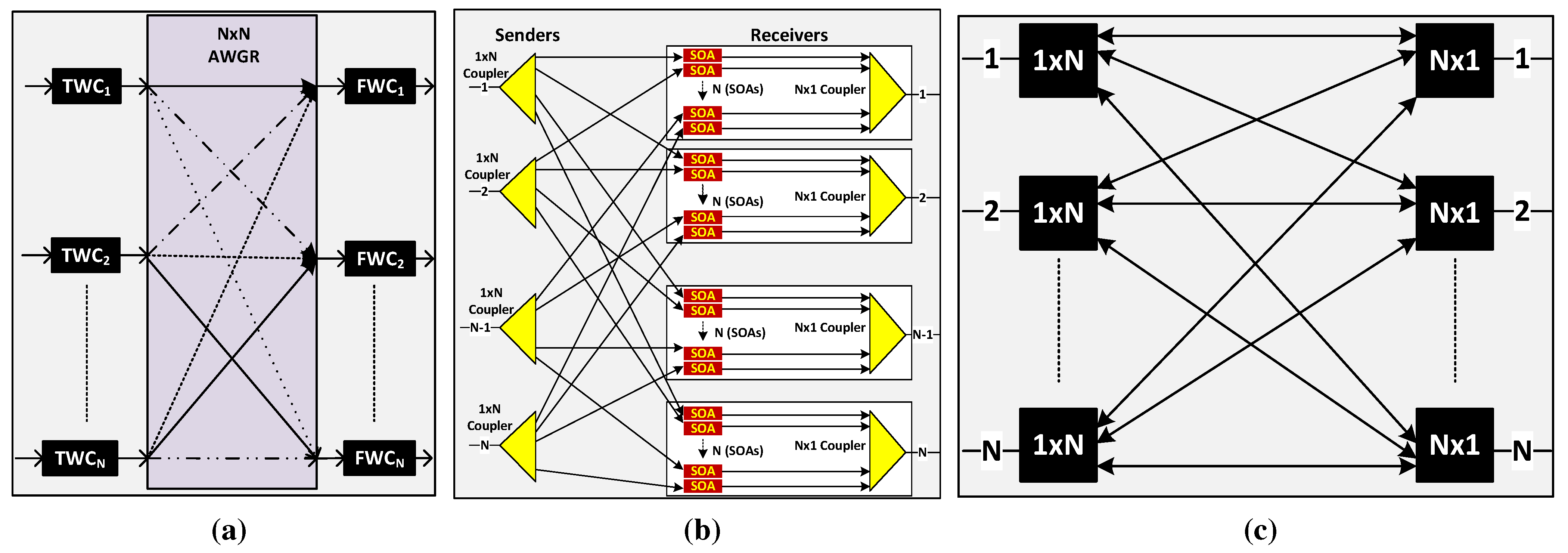
2.3.1. AWGR
An AWGR can be used as a strictly non-blocking switch, if it is used with tunable wavelength converters (TWCs) at the input ports and fixed wavelength converters (FWCs) at the output ports. Its design in shown in
Figure 2a. The TWC selects its wavelength according to the desired output port. An AWGR switch design with (512 × 512) ports has been reported by using 512 channels with 10 GHz channel spacing [
8]. AWGR-based interconnects have been proposed in recent studies [
17,
18,
19].
2.3.2. SOA Switch
An SOA switch can be built by using SOAs in a broadcast-and-select architecture [
9,
10,
20] as shown in
Figure 2b. First, the input signal is broadcast using a (1 ×
N) coupler, where
N is the total number of input/output ports. Each output of the (1 ×
N) coupler is attached to one of
N SOAs per output port. It has been reported that SOAs are required after every (1 × 32) coupling factor, in order to provide gain to overcome losses [
10]. A large scale strictly non-blocking switch fabric having (1024 × 1024) ports can be built if two stages of SOA gates are used,
i.e., after the first stage of SOAs, light is broadcast again by using a (1 × 32) coupler to another stage of SOAs.
Figure 2.
Different types of fast optical switches. (a) arrayed waveguide grating routers (AWGR) Switch; (b) emiconductor optical amplifier (SOA) Switch; (c) 1×N Photonic Switch.
Figure 2.
Different types of fast optical switches. (a) arrayed waveguide grating routers (AWGR) Switch; (b) emiconductor optical amplifier (SOA) Switch; (c) 1×N Photonic Switch.
2.3.3. (1 × N) Photonic Switch
Photonic switches with a (1 ×
N) configuration using Polarized Lead Zirconium Titanate (PLZT) waveguide technology have been proposed [
12]. These switches use (1 × 2) Mach-Zehnder Interferometer with 3dB couplers arranged in multiple stages to implement a (1 ×
N) switch fabric. A Photonic switch with a (1 ×
N) configuration using phased array switching technology has also been proposed [
21]. These switches use a single stage of phased array modulators between star couplers. An (
N ×
N) strictly non-blocking switch fabric can be built by using the Spanke architecture [
13] as shown in
Figure 2c. A (1 ×
N) switch is used at each input port and an (
N × 1) switch is used at each output port.
3. Performance Analysis
To assess the performance of the OCS for architecture described above, we developed simulations models using OMNeT
++ simulation framework [
22]. The key simulation parameters are presented in
Table 1. The simulated topology comprises 40 ToR switches with 40 servers connected to each ToR switch. We consider a management network for the control plane that connects all ToR switches with a single controller. We use one fast switch which is connected to the management network.
We consider three different core network sizes, i.e., fully subscribed, 2:1 over-subscribed and 4:1 oversubscribed networks wherein the degree of each ToR is 40, 20 and 10 respectively. The three different levels of core network oversubscription are explored so as to investigate the impact of traffic aggregation on the performance of the system. In a fully subscribed network, all servers in a rack send their traffic to the servers in other racks, i.e., 100% of the traffic is inter-rack while in a 2:1 oversubscribed network, 50% of the traffic is inter-rack and 50% of it is intra-rack. Similarly in a 4:1 oversubscribed network, 75% of the traffic is intra-rack and 25% of the traffic is inter-rack. A fully subscribed network will aggregate more traffic than 2:1 or 4:1 oversubscribed networks, resulting in higher latency due to the higher transmission time under the same parameters of traffic aggregation and load. We consider four cases for traffic aggregation by using values of aggregation in all three networks drawn from the set {25 μs, 50 μs, 75 μs, 100 μs}.
Table 1.
Simulation Parameters.
Table 1.
Simulation Parameters.
| Parameter Name | Symbol | Value |
|---|
| ToR switches & total racks | TRK | 40 |
| Servers in each rack | SRK | 40 |
| Degree of ToR switches | X | {40,20,10} |
| Traffic aggregation time | Ta | {25 μs,50 μs,75 μs,100 μs} |
| Processing time of control packet | Tproc | 1 μs |
| Switching time of fast switch | Tswf | 1 μs |
| Overhead | Toverhead | 1 μs |
| Data rate | | 10 Gbps |
| Topological degree of communication | TDC | {1,10}racks |
We use a conservative value of 1 μs for the switching time of the optical switches. Fast optical switches can be configured in a few nanoseconds [
10,
18]. The RTT of the control packet comprises its processing time at the controller (
Tproc) and the overhead time (
Toverhead). The overhead time is the sum of the propagation delay, the processing delay of the control packet at the electronic switch, and the delay in performing optical-electrical-optical (O-E-O) conversion. We conservatively select the value of
Toverhead to be 1 μs, even though all these delays are negligible (at most a few nanoseconds [
7]). We choose a value of 1 μs for
Tproc. The
Tproc is compatible with the upper bound of the routing and scheduling algorithm that we measure in
Section 4.1.
We select two cases of topological degree of communication (TDC). The TDC indicates the traffic workload diversity. Setting TDC = 1 means that servers in a rack communicate with servers in only 1 destination rack (low traffic diversity) while setting TDC = 10 indicates that each server in a rack communicates with servers in 10 destination racks (high traffic diversity).
We benchmark the performance against an ideal electrical packet switching network that features a two layer leaf-spine topology [
23] as shown in
Figure 3. Its performance provides a baseline against which to compare the performance of the new networks.
Figure 3.
Topology diagram for the baseline electrical network (Leaf-spine topology).
Figure 3.
Topology diagram for the baseline electrical network (Leaf-spine topology).
4. Results and Discussion
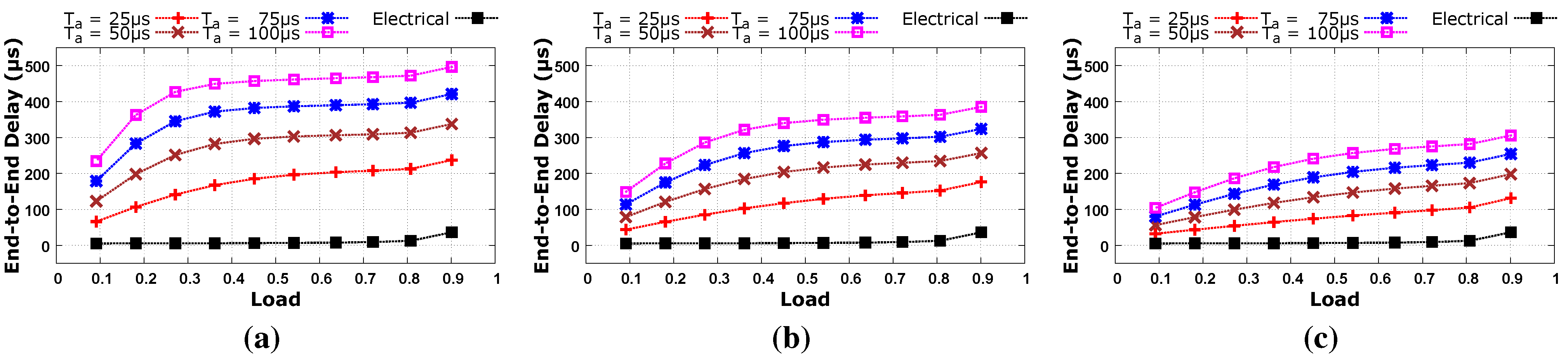
The simulation results obtained are shown in
Figure 4 and
Figure 5. Four of the curves in
Figure 4 and
Figure 5 show end-to-end delay versus offered load for different values of the traffic aggregation time while the fifth curve shows corresponding performance of the baseline electrical network.
Figure 4.
Average end-to-end latency with different parameters of traffic aggregation and with respect to different network over-subscription for low diversity traffic, i.e., topological degree of communication (TDC) = 1. (a) Fully Subscribed Network; (b) 2:1 Over-subscribed Network; (c) 4:1 Over-subscribed Network.
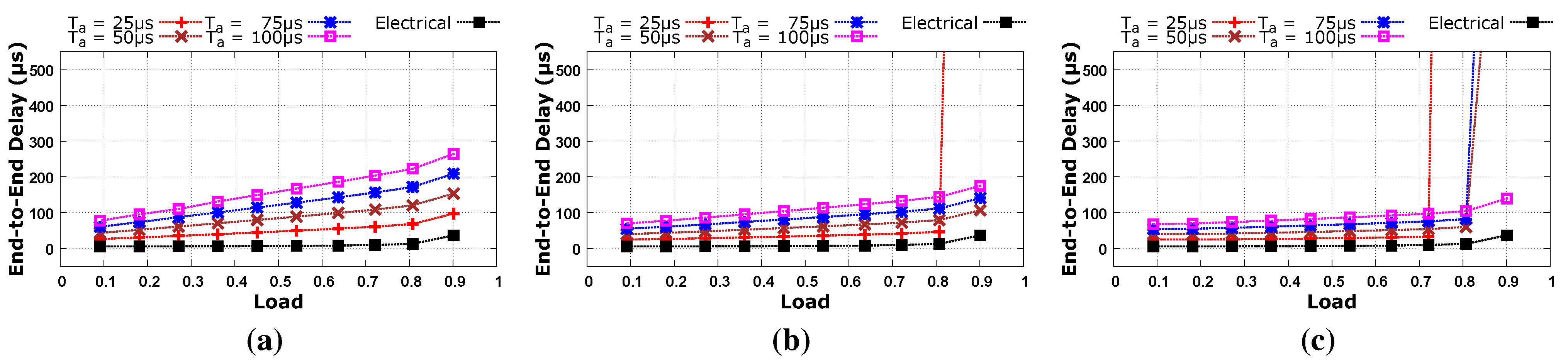
Figure 5.
Average end-to-end latency with different parameters of traffic aggregation and with respect to different network over-subscription for high diversity traffic, i.e., TDC = 10. (a) Fully Subscribed Network; (b) 2:1 Over-subscribed Network; (c) 4:1 Over-subscribed Network.
Figure 5.
Average end-to-end latency with different parameters of traffic aggregation and with respect to different network over-subscription for high diversity traffic, i.e., TDC = 10. (a) Fully Subscribed Network; (b) 2:1 Over-subscribed Network; (c) 4:1 Over-subscribed Network.
Figure 4 and
Figure 5 also reveal the impact of traffic diversity. Low diversity traffic where TDC = 1 has higher latency than high diversity traffic where TDC = 10 in a fully subscribed network as shown in
Figure 4a and
Figure 5a. This is because a large amount of traffic is aggregated with a low diversity workload, it takes more time to transmit this large amount of traffic, and so high latency is observed. Latency decreases as we move from a fully subscribed network to an oversubscribed network due to lower levels of traffic aggregation. It can be inferred from our results that aggregated traffic should not be less than 100 μs at high load levels that may result in network congestion as shown in
Figure 5b with
Ta = 25 μs and in
Figure 5c with
Ta = {25 μs, 50 μs, 75 μs}. In these cases, circuit establishment requests are generated more frequently and each request is delayed by the RTT of the control packet. Network bandwidth is wasted during this round trip time, and so network congestion may occur at high traffic load. In the case of a low traffic load, we get performance comparable to the baseline electrical network because any wasted bandwidth caused by circuit establishment requests is not so high that it could lead to network congestion.
4.1. Performance of the Control Plane
In order to assess the performance of the routing and scheduling algorithm of the control plane, we run our algorithm on an Intel host with a Core i7, 2.17 GHz processor and 16 GB RAM. The results were obtained for several combinations of parameters. To ensure statistical significance, we averaged the results of 1000 runs and the results are shown in
Table 2.
When a control packet arrives at the controller, the controller performs the routing and scheduling operations described in Algorithm 3. The complexity of the routing and scheduling algorithm is
O(
Q ×
X +
μ), where
Q is the number of optical switches,
X is the degree of ToR switches and
μ represents the sum of processing time of all other instructions. This is assumed to be a constant of negligibly low value. We measure the execution time in fully subscribed, 2:1 oversubscribed and 4:1 oversubscribed networks as shown in
Table 2. We assume 40 servers per rack and 1000 port optical switch. It can be noticed in
Table 2 that we get good performance of the algorithm in 4:1 oversubscribed networks even with a 1000 rack network. The execution time of the algorithm increases as we decrease the level of network over-subscription. A fully subscribed network is inefficient, e.g., only 40% resources of a fully subscribed fat tree network is utilized [
24]. So in order to efficiently utilize resources, network over-subscription is used. By using oversubscribed networks, our algorithm demonstrates good performance even with very high network size.
Table 2.
Performance of the Control Plane.
Table 2.
Performance of the Control Plane.
| Algorithm | Over-Subscription | Optical Switch (Q) | Degree of ToR (X) | Racks (N) | Exec. T |
|---|
| Routing and scheduling | 4:1 | 1 | 10 | 100 | <0.1 μs |
| 10 | 10 | 1000 | <0.5 μs |
| 2:1 | 1 | 20 | 50 | <0.1 μs |
| 10 | 20 | 500 | 1 μs |
| 20 | 20 | 1000 | 2.1 μs |
| 1:1 | 1 | 40 | 25 | <0.1 μs |
| 20 | 40 | 500 | 3.1 μs |
| 40 | 40 | 1000 | 6.2 μs |
4.2. Future Work
In this paper, we consider network-level simulation of a proposed new data center network design by using OMNeT++ to validate our design. In future, we aim to develop a prototype of this design. For this purpose, we aim to use servers to emulate ToR switches and another server will be used as the controller. In order to implement the control plane algorithm, there are two options: (1) To develop our own controller; (2) To use an existing SDN controller and implement our algorithm on it. For second option, different open source SDN controller can be considered such as OpenDayLight, OpenContrail, Ryu, Floodlight and FlowVisor. For data plane implementation, we can consider any fast optical switch that we describe in
Section 2.3.
5. Conclusions
We investigated the performance of a new OCS architecture for data center networks by using network-level simulation. The modelled switch architecture features fast optical switches in a single hop topology with a centralized software-defined optical control plane.
We consider circuits of short-duration and use different workloads with various traffic aggregation parameters to investigate the OCS performance. The results reveal that our traffic aggregation mechanisms, with appropriately chosen parameters, produce delay performance comparable to that of an electrical packet switched data center network even with high traffic load.


