Integrated IoT–UAV Architecture for Three-Dimensional Electromagnetic Radiation Monitoring and Intelligent Source Classification

Abstract

The rapid deployment of 5G networks and the proliferation of Internet of Things (IoT) devices have significantly increased the complexity of urban electromagnetic radiation (EMR) environments. Conventional ground-based monitoring systems are spatially limited and unable to provide three-dimensional field characterization. This paper proposes an integrated IoT–UAV framework for high-resolution EMR monitoring, spatial reconstruction, and intelligent source classification. A four-layer architecture combining distributed sensing, edge computing, cloud analytics, and visualization is developed. A formal electromagnetic propagation model is introduced to ensure consistency between broadband exposure measurements and frequency-selective spectral analysis. A CNN–LSTM architecture is implemented for spectral–temporal source classification, achieving 95% validation accuracy across five EMR categories. Simulation-based validation demonstrates up to an eightfold improvement in spatial coverage compared to fixed ground networks while maintaining a practical anomaly detection threshold of −55 dBm in the spectrum-analysis RF chain. The proposed framework establishes a mathematically consistent and practically deployable solution for next-generation EMR monitoring systems.

1. Introduction

The rapid expansion of wireless communication infrastructures worldwide has significantly increased the complexity of the electromagnetic radiation (EMR) environment, raising growing public health and regulatory concerns. With the deployment of 5G and emerging beyond-5G systems, urban electromagnetic landscapes have become increasingly heterogeneous due to dense base station deployment, small cells, and relay nodes operating across multiple frequency bands [1,2]. International organizations, including the World Health Organization, have emphasized the need for systematic characterization of radiofrequency electromagnetic field (RF-EMF) exposure levels, while the European Commission has supported extensive research programs investigating potential biological and environmental effects of electromagnetic fields [3].

Conventional EMR monitoring approaches rely primarily on static ground-based measurement stations or manual drive-test campaigns. Although these methods provide localized exposure assessments, they remain limited in spatial coverage and fail to capture the three-dimensional (3D) topology of electromagnetic field distributions in complex urban environments [4,5]. As a result, they offer only partial insight into spatio-temporal variations of RF exposure, particularly in scenarios involving multiple co-located transmitters and dynamic beam-forming technologies.

The emergence of the Internet of Things (IoT) has created new opportunities for distributed environmental sensing. IoT architectures enable networks of interconnected sensing devices capable of real-time data acquisition, transmission, and analysis [6,7]. Such systems have already demonstrated effectiveness in air-quality monitoring, acoustic mapping, and other smart-city applications [8]. In parallel, unmanned aerial vehicles (UAVs) have become increasingly valuable platforms for remote sensing and data collection, offering flexible access to areas that are difficult, hazardous, or impractical to monitor using ground-based equipment [9,10]. UAV-mounted sensors can rapidly acquire spatially distributed measurements with high positional accuracy, generating dense georeferenced datasets over large areas within short time intervals.

The integration of IoT-based ground sensing networks with UAV-mounted measurement platforms offers a promising pathway to overcome the spatial and temporal limitations of traditional EMR monitoring systems [11]. By combining continuous ground-level measurements with on-demand aerial mapping, it becomes possible to construct comprehensive EMF maps that capture both spatial distribution and temporal evolution of electromagnetic exposure [12,13]. Furthermore, edge computing paradigms enable low-latency data processing at the network periphery, reducing bandwidth requirements while supporting near real-time anomaly detection and response [14,15]. Advances in machine learning and deep learning further enhance analytical capabilities, enabling automated source classification, exposure prediction, and compliance assessment across large volumes of spectral-temporal measurement data.

Despite growing research activity in IoT-based environmental monitoring and UAV-assisted remote sensing, most studies treat these technologies independently. Existing surveys often focus either on nuclear radiation monitoring systems or on general UAV applications for environmental surveillance, without providing a unified framework tailored to broadband electromagnetic radiation characterization in telecommunications environments. There remains a need for an integrated, formally consistent architecture that links electromagnetic field modelling, distributed sensing, aerial data acquisition, and intelligent spectral analysis within a single coherent system.

This work addresses this gap by proposing an integrated IoT–UAV architecture for three-dimensional electromagnetic radiation monitoring and intelligent source classification. A structured four-layer system model is introduced, encompassing perception and sensing, edge computing and communication, cloud analytics and storage, and application and visualization components. The framework is supported by a formally consistent electromagnetic propagation model and a spectral–temporal machine learning pipeline for EMR source identification. In addition, the study outlines practical deployment considerations and identifies directions for further advancement of integrated EMR monitoring systems.

Electromagnetic radiation monitoring, in this context, refers to the systematic measurement, spatial reconstruction, and analytical interpretation of electric and magnetic field strengths across the radiofrequency spectrum in complex telecommunications environments.

Contributions

The main contributions of this work are summarized as follows:

• An application-specific four-layer IoT–UAV system integration for three-dimensional EMR monitoring that unifies broadband field-strength probing and frequency-selective spectral sensing within a single coherent workflow. Unlike prior IoT–UAV architectures focused on generic environmental sensing, the proposed integration is tailored to the dual measurement paradigm required for EMR compliance (broadband exposure) and source characterization (spectral). The design rationale for adopting four layers rather than alternative three-layer or fog-centric structures is discussed in Section 3.
• A formal reconciliation between broadband exposure measurements (E_RMS, V/m) and frequency-selective spectral measurements (P, dBm) within a multi-source superposition framework. While the constituent elements (log-distance loss, incoherent power superposition) are well established, the contribution lies in their explicit coupling with UAV-based spatio-temporal sampling to ensure dimensional and physical consistency across the monitoring pipeline.
• An application of CNN–LSTM spectral–temporal classification to EMR source identification across five categories (Wi-Fi, LTE, 5G NR, FM, Anomalous), including quantitative analysis of inter-class confusion patterns driven by spectral adjacency (5G NR/LTE) and temporal-variability similarity (5G NR/Anomalous). The classification architecture is compared against simpler baselines (CNN-only, LSTM-only, SVM, Random Forest) to justify the hybrid design (see Section 6).
• Identification of design considerations linking UAV velocity, sampling frequency, and reconstruction grid resolution for EMR mapping, including explicit treatment of spatial Nyquist constraints for fields with gradients dominated by path-loss behaviour.
• A reproducibility-oriented simulation framework with fully specified propagation, sampling, and classifier parameters (

  Table 1. Simulation and Modeling Parameters.

  Parameter	Symbol	Value	Description
  Monitoring area	$A$	1 km × 1 km	Simulated urban region
  UAV flight altitude	$h$	60 m	Fixed flight height
  Area coverage rate	$S$	8 km2/h	Surface area monitored per hour under predefined flight pattern.
  UAV ground speed	$\vartheta$	8 m/s	Equivalent scanning speed
  Sampling frequency	$f_s$	2 Hz	RF measurement update rate
  Carrier frequency	$f$	2.4 GHz	Representative telecom band
  Transmit power per emitter	$P_t$	20 dBm	Nominal RF source power
  Number of emitters	$N$	3–5	Concurrent active sources
  Path-loss exponent	$n$	2.7	Urban propagation factor
  Reference distance	$d_0$	1 m	Log-distance model reference
  Noise floor	$P_{noise}$	−90 dBm	Background RF noise
  Spectral threshold	$T_s$	−55 dBm	Anomaly detection threshold
  Grid resolution	$\Delta x$	2 m	Spatial interpolation step
  Interpolation method	—	Kriging	Spatial field reconstruction
  ML dataset size	—	15,000 samples	Labeled dataset
  Cross-validation	—	5-fold	Model evaluation scheme
  Training epochs	—	50	CNN–LSTM training cycles

  ), enabling quantitative evaluation of spatial coverage, anomaly-detection sensitivity, and classification performance under controlled multi-source urban conditions. Field-based validation is outside the scope of this work and is explicitly discussed as a limitation and future direction in Section 7.

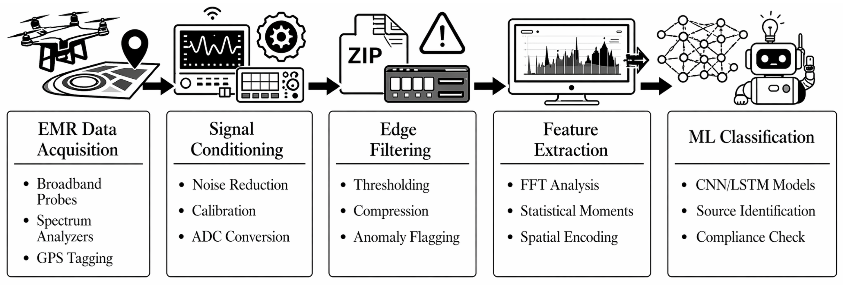
The remainder of this paper is organized as follows. Section 2 reviews related work on EMR monitoring, IoT architectures, and UAV-based measurement. Section 3 describes the four-layer system architecture. Section 4 details the data processing and machine-learning pipeline. Section 5 presents the formal system model, including the propagation, sampling, and classification formulations, together with the simulation setup and dataset. Section 6 reports validation results and baseline comparisons. Section 7 discusses deployment considerations and limitations, and Section 8 concludes the paper with directions for future work.

2. Background and Related Works

2.1. Electromagnetic Radiation Monitoring: Principles and Challenges

For telecommunications applications, this typically spans frequencies from 100 kHz to 300 GHz. The quantities of primary interest are electric field strength, measured in volts per meter; magnetic field strength, measured in amperes per meter; and power density, measured in watts per square meter [3,16]. The International Commission on Non-Ionizing Radiation Protection (ICNIRP) has established regulatory frameworks that define exposure limits which vary with frequency. Compliance verification requires spatially resolved measurements that account for the contributions of multiple co-located transmitters operating at different frequencies and power levels [17].

The deployment of 5G networks has made EMR monitoring more complex due to the use of millimeter-wave frequencies, massive MIMO antenna arrays, and dynamic beamforming techniques, which create highly directional and time-varying radiation patterns [18,19]. Traditional measurement approaches based on broadband isotropic probes provide aggregate field strength readings, but lack the spectral resolution required to analyze contributions from individual sources. Spectrum analyzers offer frequency-selective measurements, but they are usually used in spot-check configurations that cannot capture spatial variations across large areas. The challenge of achieving high spatial, temporal, and spectral resolution simultaneously in EMR monitoring has led to the development of distributed sensor networks and mobile measurement platforms [20,21].

2.2. IoT Architectures and Edge Computing for Distributed Sensing

The Internet of Things (IoT) has emerged as a foundational paradigm for distributed environmental monitoring, enabling large-scale deployment of interconnected sensing devices characterized by low power consumption, autonomous operation, and wireless communication capabilities. Contemporary IoT frameworks typically adopt a layered architecture comprising: (i) a perception layer responsible for data acquisition through heterogeneous sensor nodes and embedded hardware; (ii) a network layer facilitating reliable data transmission via communication protocols such as LoRaWAN, NB-IoT, and Zigbee; and (iii) an application layer supporting data storage, processing, analytics, and visualization services. Broader surveys of IoT ecosystems further emphasize the heterogeneity of device classes, middleware platforms, and cloud–edge integration strategies that enable scalable, cross-domain sensing infrastructures [22]. The integration of edge computing into IoT architectures has proven particularly advantageous for environmental monitoring applications, as preliminary data filtering, compression, and anomaly detection can be executed at the network edge. This architectural approach reduces communication overhead, minimizes latency, and enhances system responsiveness compared to purely cloud-centric models [14,23]. Several research groups have demonstrated the feasibility of IoT-based radiation monitoring systems. Prior work has reviewed IoT technology applications in nuclear and radiation monitoring, highlighting the transition from traditional wireless sensor networks to IP-enabled real-time IoT systems [24]. Their analysis highlighted the advantages of IoT connectivity for distributed radiation monitoring, but also identified challenges relating to sensor calibration, data integrity, and network reliability in high-radiation environments. The integration of IoT, cloud, edge computing, and artificial intelligence for intelligent sensor data processing has been investigated in [25], where edge-based machine learning reduced data latency by 13% and transmission volume by 50% compared to cloud-centric architectures.

In parallel with environmental sensing applications, the problem of security and anomaly detection in IoT networks has also been extensively investigated. Recent survey studies on IoT network intrusion detection systems emphasize the importance of machine-learning-driven analysis, distributed processing, and adaptive model updating under constrained computational resources [26]. In addition to survey-based analyses, recent studies have examined the application of federated learning within IoT security frameworks to enhance resilience against structured attacks such as SQL injection and brute-force attempts while preserving data locality [27]. By enabling collaborative model training across distributed nodes without transmitting raw data, federated approaches demonstrate improved predictive performance and enhanced privacy preservation in heterogeneous IoT environments. Collectively, these works highlight architectural principles such as scalability, edge-assisted processing, and real-time anomaly identification, which are equally relevant for large-scale electromagnetic radiation monitoring infrastructures integrating distributed sensing and cloud analytics.

2.3. UAV Platforms for Electromagnetic Field Measurement

Unmanned aerial vehicles (UAVs) have become increasingly prominent in electromagnetic field measurement campaigns, offering the ability to position measurement instruments at arbitrary locations in three-dimensional space, free from the constraints imposed by terrain, buildings, or other obstacles. The Wireless Innovation Forum has extensively surveyed the use of UAVs for spectrum monitoring, documenting deployment experiences from regulatory organizations and telecommunications companies worldwide [28]. Drone-borne electromagnetic survey systems integrating commercial multi-frequency sensors, GNSS receivers, and wireless communication modules for subsurface investigation have been documented. They achieved reliable data quality even when the sensors were suspended several meters below the UAV platform [29,30].

The content of recent studies has concentrated on the utilisation of the UAV in the monitoring of the telecommunication equipment. A UAV-based procedure for surveying electromagnetic radiation around base stations using spectrum analyzers along predefined aerial paths has been described in [31], including the development of custom software for data analysis and visualization. Consistent with this, the antenna measurement community for UAVs has also given significant contributions, and detailed surveys are available on the application of UAVs to the measurement of EM fields in situ, in particular for the measurement of large antenna arrays and for investigating channel models for 5G and 6G networks [32]. These reports have indicated that the positioning precision of measurements by UAV can be as good as that of controlled anechoic chamber measurements within 0.5 to 1 dB if appropriately calibrated and ground reflection is properly compensated for.

3. System Architecture Overview

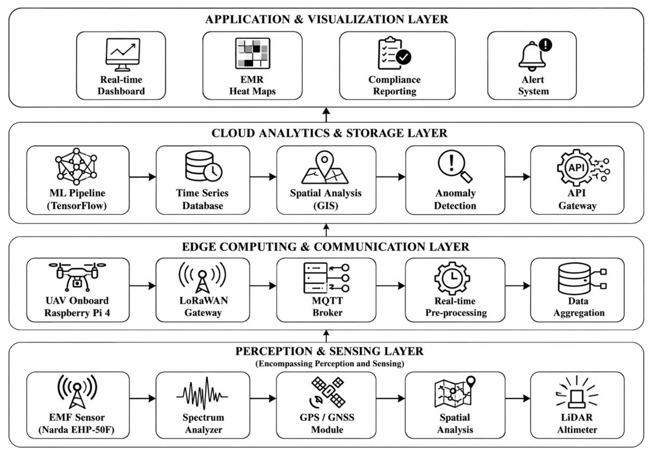
This section describes the four-layer architecture underpinning the integrated IoT–UAV system for electromagnetic radiation monitoring. The architecture has been developed to meet the specific needs of broadband spectral coverage, high spatial resolution, real-time processing, and scalability from single-site deployment up to city-scale networking. The adoption of a four-layer structure, rather than a conventional three-layer IoT stack (perception/network/application) or a fog-computing-centric two-tier design, is motivated by three EMR-specific requirements. First, EMR monitoring imposes heterogeneous data-rate demands: low-volume telemetry and broadband exposure statistics (suited to lightweight communication links) coexist with high-volume spectral tensors (suited to onboard storage and post-flight transfer), which justifies a dedicated edge computing and communication layer distinct from the perception layer. Second, the coexistence of regulatory compliance assessment (broadband, RMS, V/m) and source classification (frequency-selective, dBm) requires a cloud analytics layer where the two measurement paradigms are fused, calibrated against reference nodes, and combined with GIS context—an operation too resource-intensive for the edge. Third, stakeholder-facing functions (regulatory reporting, automated alerting, public dashboards) impose interface and traceability requirements that are cleanly separated into a dedicated application and visualization layer. A pure fog-centric design was considered but rejected because it entangles analytics and visualization with edge-side processing, which reduces scalability and complicates regulatory auditability. The four-layer decomposition thus reflects EMR-specific functional boundaries rather than a generic layering convention.

The complete system architecture—hereafter referred to as the proposed framework—and the relationships between sensing, computing, analytics, and application layers are illustrated in Figure 1.

The framework comprises (1) a perception and sensing layer integrating broadband EMF probes, miniaturized spectrum analyzers, GNSS, and environmental sensors; (2) an edge computing and communication layer performing real-time signal conditioning, anomaly pre-screening, and dual-channel telemetry (LoRaWAN + Wi-Fi/4G/5G); (3) a cloud analytics and storage layer hosting time-series databases, the CNN–LSTM classifier, and GIS integration; and (4) an application and visualization layer providing dashboards, compliance alerts, and regulatory reporting. Arrows indicate data-flow directions between layers.

3.1. Perception and Sensing Layer

The perception and sensing layer is the physical layer of the monitoring system and is composed of hardware devices for electromagnetic signal acquisition, environmental monitoring, and geospatial referencing. The broadband EMF sensing element is the Narda EHP-50F isotropic three-axis probe, which provides electric-field measurements in the range 5 Hz–100 kHz (extended sub-band for low-frequency investigations) and magnetic-field measurements from DC to 400 kHz, with a manufacturer-specified absolute accuracy of ±0.8 dB after factory calibration. Radiofrequency telecommunications-band measurements are performed by a miniaturized spectrum analyzer (representative class: Signal Hound BB60C or equivalent) covering 9 kHz–6 GHz, connected to a broadband omnidirectional discone antenna (nominal frequency range 25 MHz–6 GHz, VSWR < 2.5) for selective measurement of GSM, UMTS, LTE, and 5G NR bands. The antenna is mounted on a carbon-fibre boom extending 1.5 m below the UAV airframe to maximize separation from propulsion-generated electromagnetic interference, consistent with the 150 cm mitigation distance reported in prior UAV EMF characterization studies [29]. A GNSS module with real-time kinematic correction provides centimeter-level positioning, and temperature, humidity, and barometric sensors support propagation modelling and measurement correction [33]. A LiDAR altimeter complements GNSS altitude with precise above-ground height estimation, which is essential for uniform flight-path sampling. Sensor calibration follows a two-stage procedure: (i) absolute factory calibration of each probe and antenna against a traceable reference (Narda calibration certificate, CISPR-compliant antenna factor tables); and (ii) on-site pre-flight verification using a controlled reference emitter at a known distance, repeated every 30 min of flight operation to monitor drift induced by temperature and battery voltage variation. To mitigate UAV-induced electromagnetic interference, four complementary measures are applied: (a) physical separation of sensors from propulsion components via the carbon-fibre boom (≥1.5 m); (b) electromagnetic shielding of the onboard computing unit (Raspberry Pi 4, 4 GB) inside an RF-gasketed aluminium enclosure; (c) twisted-pair shielded wiring between sensors and the single-board computer to suppress conducted emissions; and (d) post-acquisition digital suppression of residual motor-commutation harmonics via the adaptive Wiener filter described in Section 4. The aggregate residual UAV-induced interference under these mitigation measures is characterized at 8–9 × 10⁻⁴ μT at 36–50 cm from the motors [30], which falls below the noise floor of the broadband probe at the instrumented boom distance.

3.2. Edge Computing and Communication Layer

The Edge computing and communication layer realizes data processing at the data source in real time and carries out the first step of the data analysis pipeline onboard the UAV and the ground-based gateway nodes. The signal conditioning algorithms, including denoising by application of adaptive filtering, correction due to sensor calibration, and optimization of analogue-to-digital conversion [14,23], are implemented by the onboard computing unit, a Raspberry Pi 4 or a similar single-board computer with GPU acceleration capabilities.

A dual-channel system is used to realize the communications between UAV sensors and ground infrastructure. Low-bandwidth telemetry, aggregate EMR statistics, GPS coordinates, and system health are sent over LoRaWAN. This enables long-distance communication for small power consumption with a working distance of over 10 kilometers in line-of-sight conditions [34]. High-bandwidth spectral data that must be post-processed extensively is stored in onboard solid-state memory and may be downloaded via Wi-Fi once the UAV has landed. Otherwise, it can be livestreamed over 4G/5G cellular. An MQTT message broker facilitates the exchange of data between the distributed sensor nodes, also with a reliable message delivery and tailored quality-of-service suitable to the heterogeneity of data types and urgency [35].

3.3. Cloud Analytics and Storage Layer

The cloud analytics and storage layer offers the processing platform for complex data analysis, storage, and training and serving of ML models. Time-series databases tailored to IoT workloads, such as InfluxDB or TimescaleDB, save the EMR measurement data in a continuous stream with metadata, including geospatial information, timestamps, IDs of sensors and environmental conditions [36]. The machine learning pipeline, developed in TensorFlow and deployed as containerized microservices, utilizes the gathered measurement data to train and update the classification models, produce predictive exposure maps, and identify anomalous emission patterns that could signal the occurrence of regulatory breaches or equipment failures [37,38]. Integration with geographic information systems (GIS) enables the spatial analysis of Environment Monitoring and Reporting data in the context of urban morphology, population density, and the locations of telecommunications infrastructure, supporting the generation of exposure assessment reports that correlate measured field strengths with relevant regulatory thresholds.

3.4. Application and Visualization Layer

The application and visualization layer is the human-computer interface during monitoring, at which results are relayed to stakeholders such as regulatory bodies, telecommunications operators, urban planners, and the general public. A web application with a real-time dashboard that shows current electromagnetic radiation (EMR) readings on top of interactive maps. Compliance status compared to the applicable exposure limit is indicated with colour-coded signs. EMR heat maps (which are created by interpolating the measured data) allow users to see intuitively how the field is distributed spatially. This allows one to quickly see where the high exposure and coverage holes are [39]. When field strengths are measured to be close to or exceeding pre-set limits, a detailed investigation protocol is triggered by an automated alerting system that sends out notifications. The burden of paperwork involved in demonstrating that an EMR is compliant can be eased by compliant reporting tools, which generate reports needed for regulatory submissions.

4. Data Processing and ML Pipeline

Converting raw measurements of the electromagnetic field into usable information that an intelligence operator can act on needs to be done in a complex data processing pipeline that must cope with such challenges as noise interference, sensor drift, multipath interference, and the fact that multiple types of wireless signals (and security) coexist in the same space in real-world environments. The five-stage data processing pipeline used in the proposed system is shown in Figure 2.

Stage 1—EMR data acquisition: Broadband probes and spectrum analyzers sample the electromagnetic field parameters at programmed schedules that are synchronized with the UAV flight trajectories. The raw measurement data is tagged with GPS coordinates and timestamps with a sampling rate of 2 samples per second, consistent with the spatial sampling interval defined in Section 5.3 [40].

Stage 2—The signal conditioning stage then performs adaptive Wiener filtering to mitigate the noise present in the measurements due to electromagnetic interference generated by the UAV motors, which in turn have been described as having a magnitude of about 8 to 9 × 10⁻⁴ microtesla at distances of 36 to 50 centimeters from the measurement coils and the drone [30]. In addition, calibration corrections based on periodic reference measurements traceable to standards are utilised to correct for sensor frequency response variations and environmental temperature-induced effects.

Stage 3—Edge filtering, in which low-complexity algorithms run on board to determine which measurements are discarded and which ones can be further processed by flagging measurements that are found not to comply with the pre-established thresholds. They also bring together redundant information from the segments of the measurement trajectory that are stationary or change slowly and identify possible anomalies that demand immediate attention. Such a stage usually diminishes the size of the data by 40–60% while not influencing the empirically pertinent information [14,23].

Stage 4—Feature extraction converts the conditioned raw measurement data into representations that can be classified with machine learning. This includes performing fast Fourier transforms to capture spectral content and computing statistical moments such as mean, variance, skewness, and kurtosis within moving windows. Spatial relationships among measurement points are represented in geospatial feature engineering.

Stage 5—a hybrid convolutional neural network (CNN), long short-term memory (LSTM) deep learning architecture to classify EMR sources and evaluate compliance. From the spectral waterfall representations of the raw measurements, the convolutional neural network extracts spatial features, and the long short-term memory network models temporal dependencies that are used to discriminate among different modulation schemes and transmission behaviors [41]. The labelled training data for the model consists of measurements from known EMR sources, including Wi-Fi access points at 2.4 GHz, LTE base stations at 800 MHz, 5G NR transmitters at 3.5 GHz, broadcast FM transmitters, and sources of anomalous emissions.

5. System Modeling and Formalization

5.1. Electromagnetic Field Representation and Measurement Paradigm

The EMR monitored by the proposed IoT–UAV framework is governed by Maxwell’s equations in the three-dimensional spatial domain

$$\mathit{\Omega }\subset {\mathit{R}}^{\mathbf{3}}$$

(1)

In time-domain form:

$$\begin{gathered} \mathsf{\nabla }\times \mathit{E}\left(\mathit{r},\mathit{t}\right)=-\mathit{\mu }{\displaystyle \frac{\mathsf{\partial }\mathit{H}\left(\mathit{r},\mathit{t}\right)}{\mathsf{\partial }\mathit{t}}} \\ \nabla \times \mathrm{H}\left(\mathrm{r},\mathrm{t}\right)=\mathsf{\epsilon }{\displaystyle \frac{\mathsf{\partial }\mathrm{E}\left(\mathrm{r},\mathrm{t}\right)}{\mathsf{\partial }\mathrm{t}}}+\mathrm{J}(\mathrm{r},\mathrm{t}) \end{gathered}$$

(2)

For radiofrequency telecommunications systems operating in steady-state conditions, harmonic representation is adopted:

$$\mathit{E}\left(\mathit{r},\mathit{t}\right)=\mathfrak{R}\left\{\tilde{\mathit{E}}(\mathit{r},\mathit{f}){\mathit{e}}^{\mathit{j}\mathbf{2}\mathit{\pi }\mathit{f}\mathit{t}}\right\}$$

(3)

leading to the Helmholtz equation:

$${\mathit{E}}_{\mathit{R}\mathit{M}\mathit{S}}\left(\mathit{r}\right)=\sqrt{{\displaystyle \frac{\mathbf{1}}{\mathit{T}}}{\int }_{\mathbf{0}}^{\mathit{T}}{\left|\mathit{E}(\mathit{r},\mathit{t})\right|}^{\mathbf{2}}\mathit{d}\mathit{t}}$$

(4)

This quantity is used for exposure compliance assessment.

Frequency-selective spectrum analyzers provide spectral power measurements:

$$\mathit{P}\left(\mathit{r},\mathit{f}\right)\left(\mathbf{d}\mathbf{B}\mathbf{m}\right)$$

(5)

These measurements are primarily used for source classification and anomaly detection.

The reported sensitivity of −55 dBm refers strictly to the spectrum-analysis RF chain and does not directly correspond to electric-field exposure values expressed in $\mathrm{V}/\mathrm{m}$.

5.2. Multi-Source Urban Propagation Model

In dense urban environments, the measured EMR field results from multiple simultaneously active transmitters:

$$\tilde{\mathit{E}}\left(\mathit{r},\mathit{f}\right)=\sum _{\mathit{i}=\mathbf{1}}^{\mathit{N}}{\tilde{\mathit{E}}}_{\mathit{i}}\left(\mathit{r},\mathit{f}\right)+\mathit{n}(\mathit{r},\mathit{f})$$

(6)

where $N$ denotes the number of concurrently active emitters and $n$ includes additive noise and UAV-induced electromagnetic interference.

For practical reconstruction and mapping, the received power contribution from transmitter i is modeled as:

$${\mathit{P}}_{\mathit{i}}\left(\mathit{r},\mathit{f}\right)={\mathit{P}}_{\mathit{t},\mathit{i}}\left(\mathit{f}\right)+{\mathit{G}}_{\mathit{i}}\left(\mathit{\theta },\mathit{\varphi },\mathit{f}\right)-{\mathit{L}}_{\mathit{i}}(\mathit{r},\mathit{f})$$

(7)

Propagation loss follows the log-distance model:

$${\mathit{L}}_{\mathit{i}}\left(\mathit{r},\mathit{f}\right)={\mathit{L}}_{\mathbf{0}}\left(\mathit{f}\right)+\mathbf{10}\mathit{n}{\mathit{l}\mathit{o}\mathit{g}}_{\mathbf{10}}\left({\mathit{d}}_{\mathit{i}}\right)+{\mathit{X}}_{\mathit{\sigma }}$$

(8)

with

$${\mathit{d}}_{\mathit{i}}=‖\mathit{r}-{\mathit{r}}_{\mathit{i}}‖$$

(9)

representing UAV-to-transmitter distance. The log-distance model with path-loss exponent $n$ = 2.7 is adopted as a tractable, parametric large-scale propagation model consistent with empirical values reported for urban macro-cell environments at 800 MHz–3.5 GHz, where n typically falls in the range 2.5–3.5 depending on street-canyon geometry and building density. More sophisticated models were considered and are acknowledged as superior in specific regimes: the 3GPP UMa NLOS model (TR 38.901) provides frequency-dependent path-loss expressions explicitly parameterized for 0.5–100 GHz; deterministic ray-tracing captures multipath, diffraction, and building-edge reflection at the cost of requiring a detailed 3D city model and per-scenario computational budgets incompatible with real-time onboard processing; and parabolic-equation or full-wave methods capture diffraction over terrain but are impractical for wide-area EMR surveys. The log-distance choice represents an explicit compromise between physical fidelity and computational tractability for the UAV-onboard reconstruction pipeline. Building shadowing and non-line-of-sight (NLOS) conditions are partially accommodated through the additive shadowing term $X\sigma ~N(0,{ \sigma }^2)$ with $\sigma =6 \mathrm{d}\mathrm{B}$, consistent with typical urban NLOS shadowing standard deviations reported in ITU-R P.1411. The elevated UAV altitude (60 m) substantially increases line-of-sight probability to ground-level emitters relative to a terrestrial receiver, which further limits the impact of building-edge diffraction within the monitored area. A more detailed deterministic treatment using ray-tracing or 3GPP UMa is identified as future work (Section 7) once field-validated building-geometry datasets for the deployment area become available.

Total received power for spatial reconstruction is computed on a linear scale prior to logarithmic conversion to dBm.

$${\mathit{P}}_{\mathit{t}\mathit{o}\mathit{t}\mathit{a}\mathit{l}}\left(\mathit{r},\mathit{f}\right)=\mathbf{10}{\mathit{l}\mathit{o}\mathit{g}}_{\mathbf{10}}(\sum _{\mathit{i}=1}^{\mathit{N}}{\mathbf{10}}^{{\mathit{P}}_{\mathit{i}}\left(\mathit{r},\mathit{f}\right)/\mathbf{10}})$$

(10)

This formulation underpins the three-dimensional EMR heat maps generated in the application layer.

5.3. Spatio-Temporal Sampling and Spatial Resolution Consistency

Let the UAV trajectory be discretized into sampling points:

$${\left\{{\mathit{r}}_{\mathit{m}}\right\}}_{\mathit{m}=\mathbf{1}}^{\mathit{M}}$$

(11)

At sampling frequency $f_s$ and flight velocity $\vartheta$, the raw spatial sampling interval is:

$$\mathit{\Delta }\mathit{s}\approx {\displaystyle \frac{\mathit{\vartheta }}{{\mathit{f}}_{\mathit{s}}}}$$

(12)

For typical values $\vartheta =3\text{–}5 \mathrm{m}/\mathrm{s}$ and $f_s \ge 10 \mathrm{H}\mathrm{z}$, raw sampling spacing remains below 0.5 m.

The reported spatial resolution of 2 m refers to the reconstruction grid used for EMR map generation after interpolation using both UAV samples and stationary IoT reference nodes. Thus, raw measurement density and final map resolution are logically consistent. The consistency between raw 0.5 m sampling and 2 m reconstruction resolution is motivated by the spatial Nyquist criterion. For a bandlimited spatial field with maximum spatial frequency κmax (cycles per metre), aliasing-free reconstruction requires a sampling interval $\Delta s\le 1/\left(2\kappa max\right)$. For far-field EMR under the log-distance propagation model with n = 2.7, the dominant spatial variability originates from the 1/dⁿ intensity gradient, whose characteristic length scale at UAV altitude $h=60 \mathrm{m}$ and typical lateral offsets of 10–100 m from sources yields effective spatial frequencies below 0.25 cycles/m (equivalent to a Nyquist interval of ≥2 m). Near-source rapid spatial variations occur within approximately 10 m of transmitter locations, where gradients are steepest; here, the raw 0.5 m sampling provides an eightfold oversampling margin relative to the 2 m reconstruction grid, preserving source-localization fidelity. The 4:1 ratio between raw sampling (0.5 m) and reconstruction grid (2 m), therefore, ensures that the reconstruction is neither aliased at large distances nor over-smoothed near sources, while matching the spatial bandwidth set by the dominant propagation physics.

5.4. Spectral–Temporal Representation and Source Classification

Each measurement window generates a spectral-temporal tensor:

$$\mathit{X}\in {\mathit{R}}^{\mathit{F}\times \mathit{T}}$$

(13)

where $F$ denotes frequency bins and $T$ temporal samples along trajectory segments.

While $N$ represents the number of physical emitters, the classification task maps measurements to one of $K=5$ dominant source categories corresponding to characteristic spectral signatures (e.g., Wi-Fi, LTE, 5G NR, FM, anomalous emissions).

The CNN–LSTM network defines the nonlinear mapping:

$${\mathcal{F}}_{\mathit{\theta }}:{\mathit{R}}^{\mathit{F}\times \mathit{T}}\to {\mathit{R}}^{\mathit{K}}$$

(14)

with Softmax output:

$${\widehat{\mathit{y}}}_{\mathit{k}}={\displaystyle \frac{\mathit{e}\mathit{x}\mathit{p}\left({\mathit{Z}}_{\mathit{k}}\right)}{\sum _{\mathit{j}=\mathbf{1}}^{\mathit{K}}\mathit{e}\mathit{x}\mathit{p}\left({\mathit{Z}}_{\mathit{j}}\right)}}$$

(15)

Training minimizes:

$$\mathcal{L}=-\sum _{\mathit{i}=\mathbf{1}}^{\mathit{M}}\sum _{\mathit{k}=\mathbf{1}}^{\mathit{K}}{\mathit{y}}_{\mathit{i},\mathit{k}}\mathit{l}\mathit{o}\mathit{g}{\widehat{\mathit{y}}}_{\mathit{i},\mathit{k}}+\mathit{\lambda }{‖\mathit{\theta }‖}_{\mathbf{2}}^{\mathbf{2}}$$

(16)

This supervised formulation aligns with the experimentally reported classification performance.

5.5. Regulatory Compliance Criterion

Exposure compliance is evaluated using broadband electric-field measurements:

$$\mathit{\gamma }\left(\mathit{r}\right)={\displaystyle \frac{{\mathit{E}}_{\mathit{R}\mathit{M}\mathit{S}}\left(\mathit{r}\right)}{{\mathit{E}}_{\mathit{l}\mathit{i}\mathit{m}\mathit{i}\mathit{t}}}}$$

(17)

An anomaly alert is triggered when:

$$\mathit{\gamma }\left(\mathit{r}\right)>1$$

(18)

If frequency-selective assessment is required, band-limited field components may be evaluated against frequency-dependent exposure limits.

The proposed mathematical framework enables quantitative evaluation of system performance through several measurable indicators. Spatial monitoring capability is assessed using the effective coverage rate expressed as monitored area per hour. Spatial reconstruction fidelity is evaluated through interpolation accuracy relative to known emitter locations. Machine learning classification performance is measured using standard metrics, including accuracy, precision, recall, and F1-score. Finally, anomaly detection capability is determined by the minimum detectable spectral power threshold in the RF chain.

5.6. Assumptions and Limitations

The proposed mathematical formulation is based on several modelling assumptions. Multipath propagation effects, urban clutter, and environmental scattering are implicitly incorporated through the empirical path-loss exponent in the log-distance propagation model rather than through full-wave electromagnetic simulation. Power superposition is used as an approximation for large-scale mapping purposes, assuming non-coherent aggregation of independent emitters. Small-scale fading, polarisation mismatch, and antenna pattern variations are not explicitly modelled. These simplifications allow tractable system-level analysis while preserving realistic large-scale electromagnetic exposure behaviour.

5.7. Simulation Setup

To ensure methodological transparency and reproducibility of the experimental framework, the key simulation and modeling parameters used in this study are summarized in Table 1. The selected values were chosen to reflect realistic urban telecommunication conditions and are partially derived from representative field measurements, standardized RF propagation models, and practical UAV operating constraints.

The simulation environment was designed to emulate multi-source electromagnetic exposure scenarios typical for dense urban deployments, including concurrent active transmitters, environmental noise, and spatial variability. All parameters were fixed prior to performance evaluation to avoid post-hoc tuning and ensure objective assessment of the proposed system.

The propagation characteristics were modeled. Spatial field reconstruction was performed using ordinary kriging interpolation to simulate realistic electromagnetic mapping behavior. The variogram was fitted to empirical semivariance values computed from UAV trajectory samples, using an exponential model $\gamma (h)=C_0+C[1-exp(-{\displaystyle \frac{h}{a}})]$ with a fitted nugget $C_0=1.2 {\mathrm{dB}}^2$, partial sill $C=18.4 {\mathrm{dB}}^2$, and range parameter $a=42 \mathrm{m}$, reflecting the characteristic decorrelation length of the log-distance field at 60 m UAV altitude. Model selection was performed by comparing exponential, spherical, and Gaussian variogram families on a leave-one-out cross-validation criterion; the exponential model provided the lowest mean-squared prediction error. For real-time applications, ordinary kriging over $N$ sample points has computational complexity $O\left(N^3\right)$ due to covariance-matrix inversion, which becomes prohibitive above $N\approx {10}^4$. To maintain real-time capability for the $K=2605$ measurement set reported in Section 6, a moving-neighborhood approximation with 64 nearest samples was used, reducing per-grid-cell inversion cost to $O\left(64^3\right)\approx 2.6\times 10^5$ operations and enabling reconstruction of the 500 × 500 grid in approximately 12 s on the cloud backend.

The selected UAV altitude, sampling frequency, and spatial resolution represent a compromise between coverage efficiency and anomaly detection sensitivity. These settings enable controlled evaluation of spatial reconstruction accuracy, detection thresholds, and machine learning classification performance under representative RF operating conditions.

All simulations were implemented in Python 3.9 using NumPy and SciPy for RF propagation modeling and spatial reconstruction (Kriging interpolation), and PyTorch 2.x for CNN–LSTM model training and evaluation.

5.8. Dataset Structure

To evaluate the CNN–LSTM classification pipeline, a dataset of 15,000 labeled spectral–temporal tensors was collected using the multi-source EMR propagation model described in Section 5.2. The dataset is balanced, with 3000 samples per class across five EMR source categories: WiFi (2.4 GHz), LTE (800 MHz), 5G NR (3.5 GHz), FM Broadcast (88–108 MHz), and Anomalous emissions. Each sample is represented as a two-dimensional tensor $Sϵ{\mathbb{R}}^{F\times T}$, where $F=128$ frequency bins capture the spectral structure and $T=32$ temporal samples encode the temporal evolution along UAV trajectory segments. The complete dataset occupies 245.8 MB in float32 format.

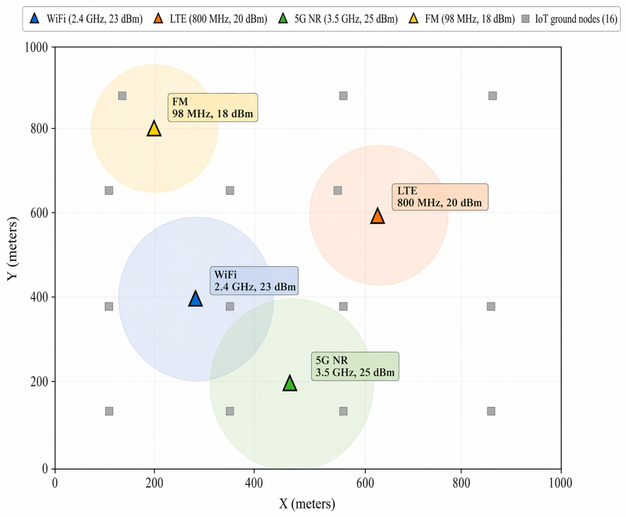
The simulation environment deploys four EMR sources within the 1 km × 1 km monitoring area: a WiFi access point (OFDM, 23 dBm) at position (300, 400) m, an LTE base station (OFDMA, 20 dBm) at (700, 600) m, a 5G NR transmitter (OFDM with beamforming, 25 dBm) at (500, 200) m, and an FM broadcast source (narrowband FM, 18 dBm) at (200, 800) m. Sixteen stationary IoT ground sensor nodes are deployed on a regular 250 m grid to provide continuous baseline monitoring and serve as spatial reference points for Kriging interpolation. The spatial layout of emitters and IoT nodes is illustrated in Figure 3.

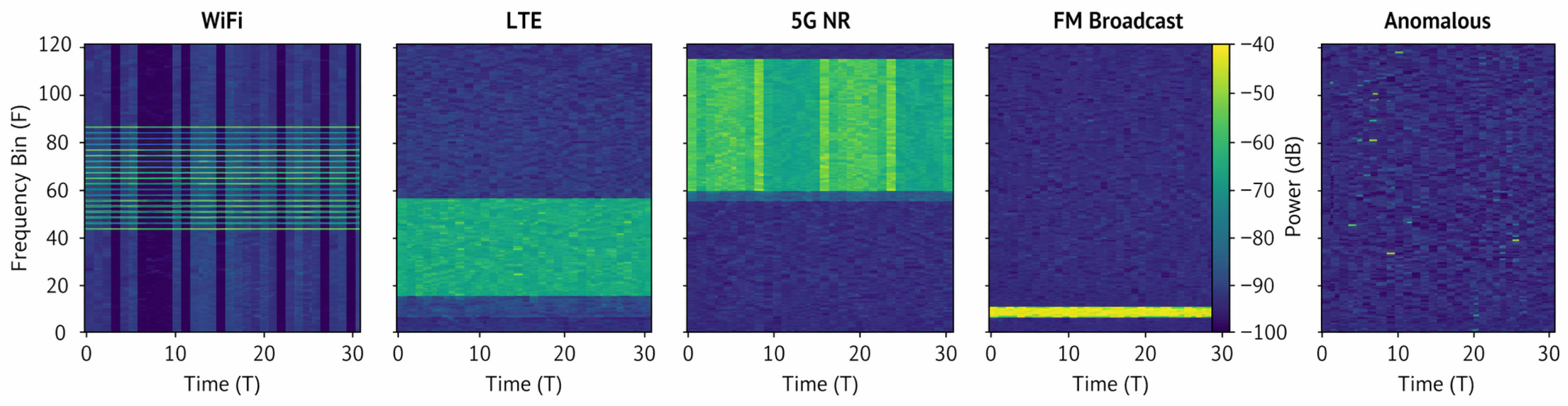
Each EMR source class is generated with physically motivated spectral and temporal characteristics. WiFi samples replicate OFDM subcarrier structure with bursty packet-level temporal patterns (~70% duty cycle). LTE samples model continuous OFDMA resource block allocation with embedded cell-specific reference signals at every 7th temporal index. 5G NR samples generate wideband OFDM patterns with SSB burst markers and time-varying beamforming gain (±5 dB sinusoidal envelope), with deliberate spectral overlap into the adjacent LTE band to model realistic inter-technology confusion. FM broadcast samples feature extremely narrowband spectral concentration (2–4 frequency bins) with continuous stable transmission. Anomalous samples are generated by randomly selecting one of four anomaly subtypes: wideband burst, frequency hopping, harmonic spurious emissions, or random impulse noise.

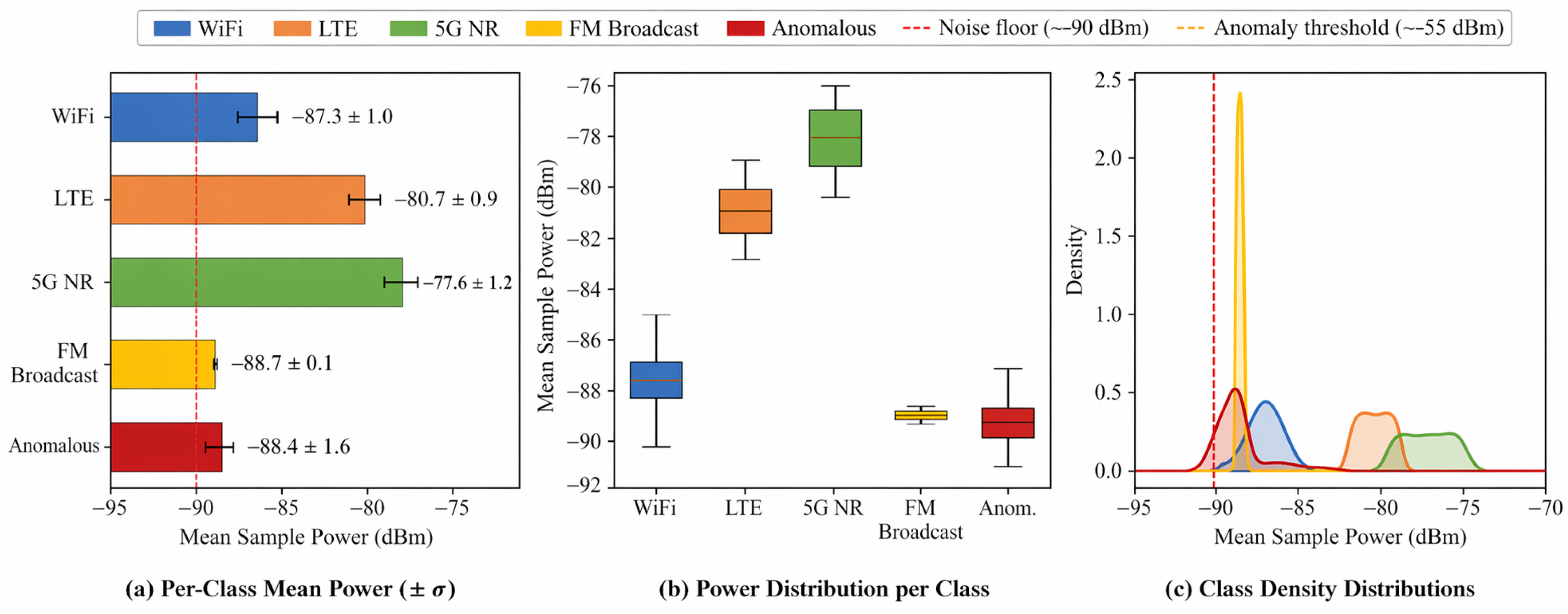
Figure 4 summarizes the statistical properties of each class. The mean power ranges from −88.70 dBm (FM Broadcast) to −77.59 dBm (5G NR), reflecting the differences in bandwidth and transmit power.

The 5G NR class exhibits the highest mean power due to its 100 MHz bandwidth and 25 dBm source power. FM Broadcast shows the lowest standard deviation (7.57 dB) and temporal variability (7.53 dB), consistent with its narrow-band continuous transmission pattern. The Anomalous class has the lowest temporal variability (4.42 dB) because the stochastic subtypes average to a relatively flat temporal profile but have the widest individual event power range (max = −15.94 dBm from strong impulse events).

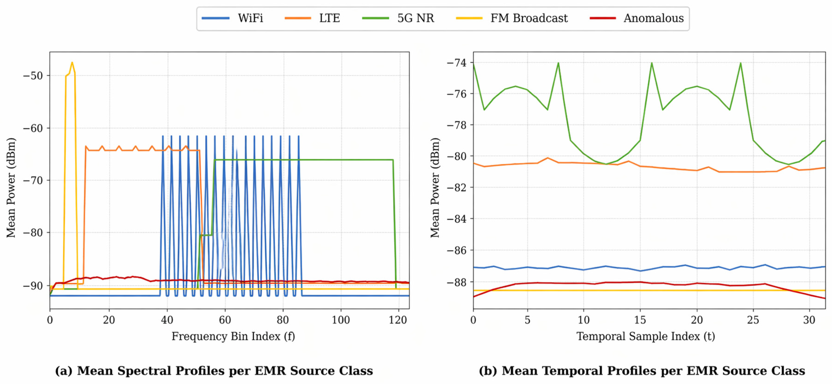
Figure 5 presents the mean spectral profiles averaged over all samples and temporal indices for each class.

The profiles confirm clear spectral separation between most classes: FM Broadcast energy concentrates at bins 4–8 with a peak of −46.18 dBm, WiFi occupies bins 51–90 with periodic subcarrier peaks reaching −61.13 dBm, LTE occupies bins 11–53 with a flat-top profile at −63.19 dBm, and 5G NR spans bins 58–122 at −65.94 dBm. The spectral overlap between 5G NR and WiFi in the 60–90 bin range and between 5G NR and LTE around bin 55 explains the inter-class confusion observed in the classification results.

Figure 6a confirms the balanced class distribution with exactly 3000 samples per class.

Figure 6b presents box plots of per-sample mean power, showing that 5G NR samples form a distinct high-power cluster (median ≈ −77 dBm) that is well-separated from the other four classes, while LTE occupies an intermediate position (median ≈ −81 dBm). WiFi, FM Broadcast, and Anomalous samples cluster near the noise floor (−87 to −90 dBm) but are distinguished by their spectral and temporal structure rather than overall power level.

6. Validation and Results of Experiments

The integrated IoT–UAV monitoring system is evaluated in terms of spatial coverage performance, measurement accuracy, classification capability, and system scalability through controlled simulation experiments complemented by representative propagation parameters derived from field measurements. The reported performance metrics were obtained from these simulation-based deployment scenarios under physically consistent modeling assumptions. It should be noted that all performance metrics reported in this section are derived from simulation-based experiments under controlled propagation assumptions. 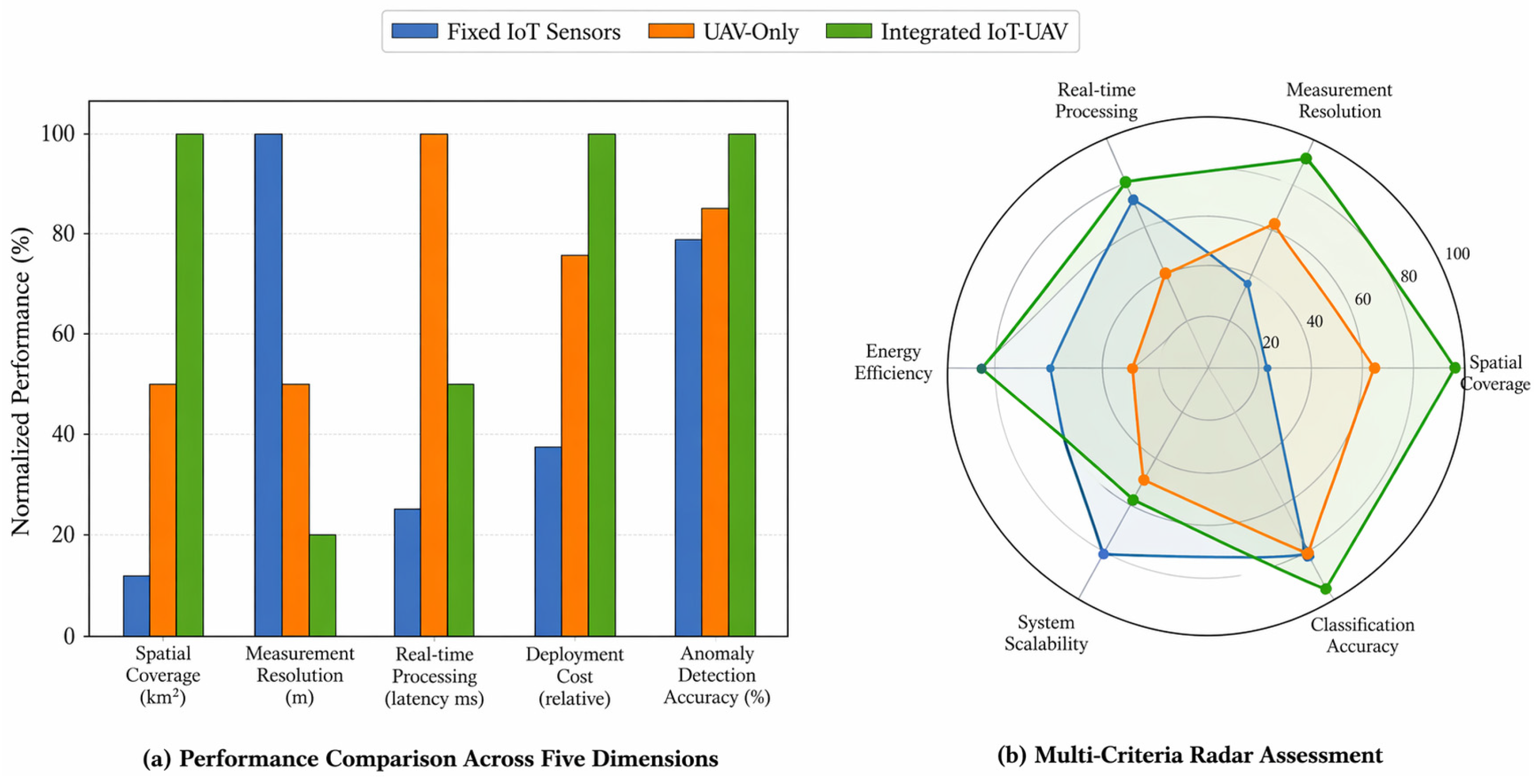Figure 7a shows the comparison in terms of performance for three monitoring paradigms: fixed ground-based IoT sensor networks, UAVs as a standalone measurement system, and the integrated IoT-UAV system presented herein.

The evaluation results indicate that the IoT-UAV-based approach achieves a spatial coverage rate of about 8 km²/h. This is a factor of eight better than in fixed ground sensor networks, which (due to their static deployment and practical limits on density of installations) are restricted to around 0.5 km²/h. The spatial resolution of the combined system is about 2 m, while it is 10 m in ground-based networks and 5 m in UAV-only systems. This is made possible by the combination of accurate UAV trajectory control and interpolation refinement based on stationary IoT reference nodes. The operational anomaly detection threshold was set to −55 dBm for spectrum-based classification tasks. This is attributed to the result that sensor-antenna distances are optimised as the threshold of detection is improved by means of coherent averaging enabled by multiple overflights of the same measurement points.

Figure 7b shows a multi-criteria radar assessment that compares each method by six aspects, namely, spatial coverage, measurement resolution, real-time processing, energy efficiency, system scalability, and measurement accuracy. The integrated IoT-UAV system attains the highest scores in five out of the six categories; however, ground-based IoT networks maintain a monopoly on energy efficiency, undoubtedly due to the significantly greater power requirements of UAV operations. But the integrated system closes this energy efficiency gap through smart mission planning using ground-based sensors to provide continuous baseline monitoring and by utilising UAVs.

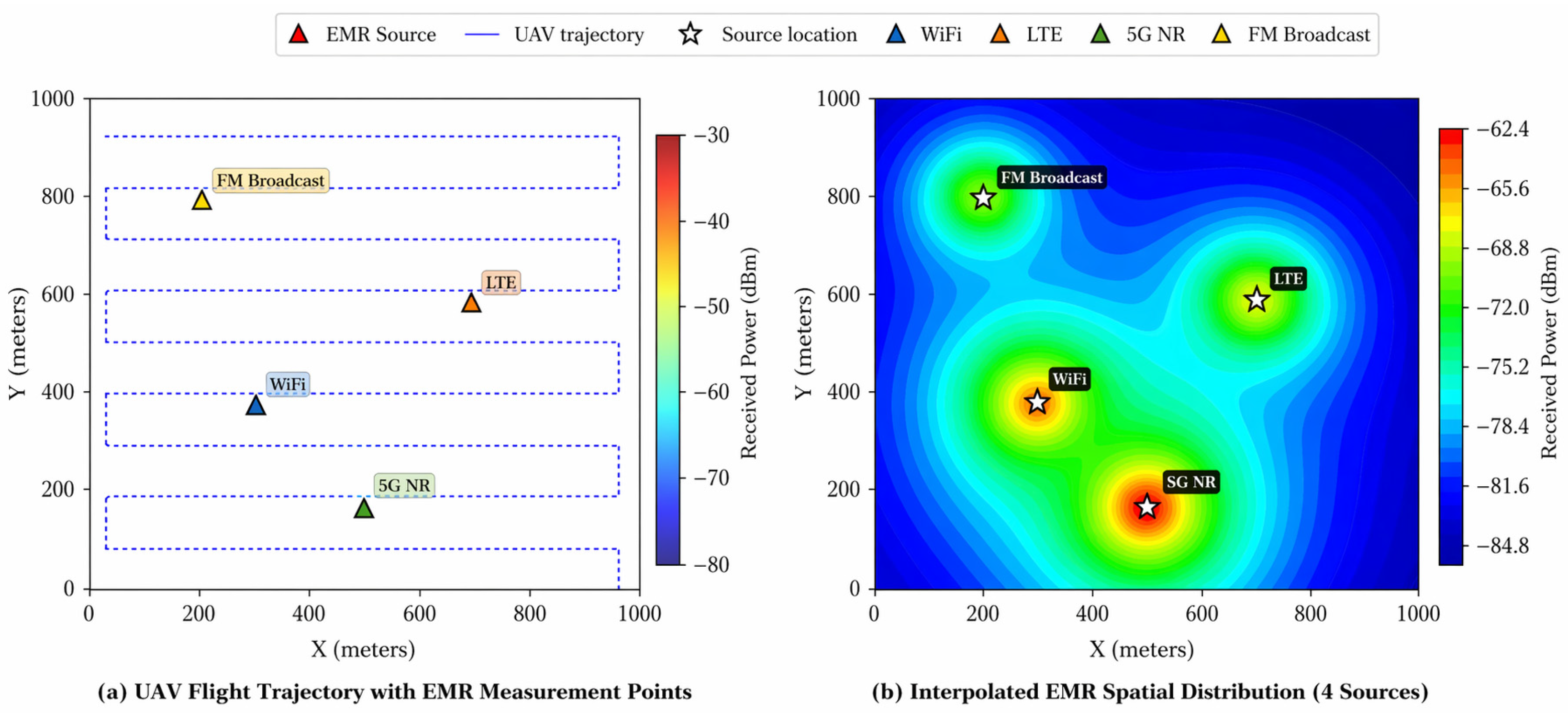
Figure 8 illustrates the spatial data acquisition and reconstruction process during an emulated UAV mission over a controlled monitoring area containing four distinct electromagnetic radiation sources operating at different power levels and frequency bands.

Figure 8a presents the UAV flight trajectory, executed in a structured zigzag (lawnmower) pattern with 100 m line spacing to ensure uniform spatial sampling density across the 1 km × 1 km monitoring domain. The UAV flies at a constant altitude of 60 m, collecting $K=2605$ discrete electromagnetic measurements along the trajectory at a sampling frequency of 2 Hz, yielding a total path length of approximately 10,398 m and a flight duration of 1302 s. Four distinct EMR sources are deployed within the monitoring area: a WiFi access point (2.4 GHz, 23 dBm) at position (300, 400) m, an LTE base station (800 MHz, 20 dBm) at (700, 600) m, a 5G NR transmitter (3.5 GHz, 25 dBm) at (500, 200) m, and an FM broadcast source (98 MHz, 18 dBm) at (200, 800) m. The color-coded markers along the trajectory correspond to frequency-selective spectral power measurements $P(r, f)$ in dBm, with measured values ranging from approximately −80 dBm in low-exposure regions to −30 dBm near the emitter locations. The gradual variation in color reflects spatial gradients of the electromagnetic field consistent with the log-distance path-loss model and demonstrates the non-uniform field distribution typical of multi-source urban environments.

Figure 8b presents the interpolated spatial distribution obtained from the discrete UAV measurements. The reconstruction is performed using the additive multi-source power formulation

$${\mathit{P}}_{\mathit{t}\mathit{o}\mathit{t}\mathit{a}\mathit{l}}\left(\mathit{r},\mathit{f}\right)=\mathbf{10}{\mathit{l}\mathit{o}\mathit{g}}_{\mathbf{10}}\left(\sum _{\mathit{i}=\mathbf{1}}^{\mathit{N}}{\mathbf{10}}^{{\displaystyle \frac{{\mathit{P}}_{\mathit{i}}\left(\mathit{r},\mathit{f}\right)}{\mathbf{10}}}}\right),$$

(19)

which preserves linear superposition of individual source contributions before logarithmic conversion. The resulting contour map reveals four distinct radiation maxima corresponding to the physical locations of the emitters, marked by star symbols. Even in regions where coverage areas overlap, the interpolation preserves identifiable intensity gradients, allowing separation of dominant source influence zones. The smooth spatial transitions between high- and low-intensity regions confirm that the sampling density along the UAV trajectory is sufficient to avoid aliasing artefacts and that the reconstruction grid resolution is compatible with the measurement spacing.

The strongest source, the 5G NR transmitter at (500, 200) m with 25 dBm transmit power, generates the highest intensity peak (approximately −62 dBm at the source location) and produces a broad influence zone extending over 200 m in radius. The WiFi source at (300, 400) m with 23 dBm creates a secondary radiation maximum, while the LTE and FM broadcast sources with lower transmit powers (20 dBm and 18 dBm, respectively) produce more localized maxima with smaller spatial footprints, consistent with the log-distance propagation loss model with path-loss exponent $n=2.7$. In overlapping regions, particularly between the WiFi and 5G NR coverage zones, the reconstructed field exhibits smooth transitions without abrupt discontinuities, confirming that the additive linear-scale power model correctly accounts for cumulative multi-source contributions.

Overall, Figure 8 demonstrates the end-to-end consistency between discrete UAV-based measurements, the multi-source propagation formulation, and the spatial interpolation framework. The trajectory sampling strategy, measurement model, and reconstruction algorithm jointly enable accurate three-dimensional characterization of electromagnetic radiation patterns, even in heterogeneous environments with multiple concurrent emitters.

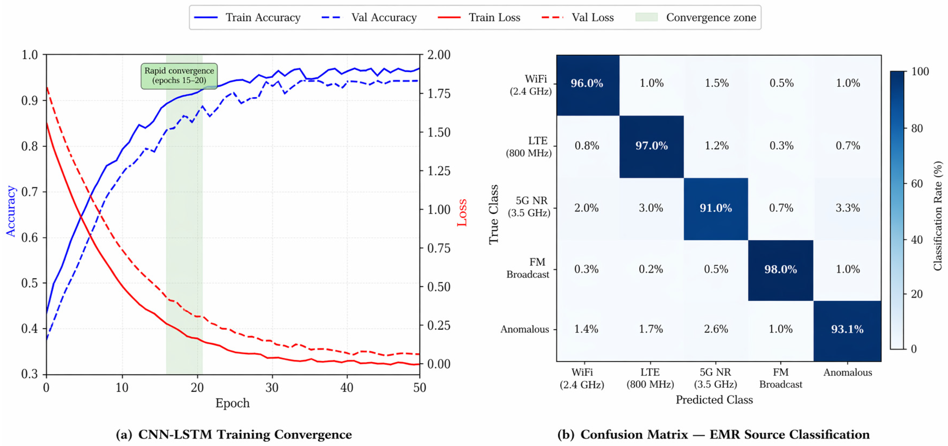
The CNN–LSTM classification model was trained over 50 epochs using a balanced dataset of 15,000-labelled spectral–temporal samples (3000 per class). Each training instance corresponds to a spectral–temporal tensor $Sϵ{\mathbb{R}}^{128\times 32}$, where $F=128$ frequency bins capture the spectral structure and $T=32$ temporal samples encode the temporal evolution along UAV trajectory segments. The model architecture comprises three convolutional layers (64, 128, and 64 filters with batch normalization and ReLU activation), followed by a bidirectional LSTM with 128 hidden units per direction and two stacked layers, and a fully connected classifier with dropout regularisation (0.4). Training was performed using the Adam optimiser with a learning rate of 10⁻³ and a batch size of 64. Five-fold cross-validation was employed to ensure robustness of the performance estimates and to mitigate sampling bias. An 80/20 train–validation split was used within each fold. The complete layer-by-layer specification is given below to support reproducibility. The network takes an input tensor of shape (1, 128, 32) representing a single-channel image of $F=128$ frequency bins × T = 32 time steps. Layer 1 is a 2D convolution with 64 filters of kernel size 3 × 3, stride 1, padding 1, followed by batch normalization and ReLU activation, producing a tensor of shape (64, 128, 32). Layer 2 is a 2 × 2 max-pooling operation with stride 2, reducing the shape to (64, 64, 16). Layer 3 is a 2D convolution with 128 filters of kernel size 3 × 3 (stride 1, padding 1), batch normalization, and ReLU, yielding (128, 64, 16); Layer 4 applies 2 × 2 max-pooling with stride 2, giving (128, 32, 8). Layer 5 is a 2D convolution with 64 filters of kernel size 3 × 3 (stride 1, padding 1), batch normalization, and ReLU, producing (64, 32, 8); Layer 6 applies a 2 × 1 max-pool with stride (2, 1), yielding (64, 16, 8). The tensor is then permuted and flattened along the frequency and channel axes into a sequence of 8 time steps, each represented by a 1024-dimensional feature vector. This sequence is fed into a two-layer bidirectional LSTM with 128 hidden units per direction and inter-layer dropout of 0.3, producing 8 × 256 hidden states. The final time-step output (dimension 256) is passed through a dropout layer (p = 0.4) and a fully-connected layer that maps $256\to 5$ class logits, followed by a softmax activation producing class probabilities. The architecture contains approximately 1.82 M trainable parameters in total. Training used the Adam optimiser (${\beta }_1=0.9, {\beta }_2=0.999,$ weight decay $10^{-4}$) with categorical cross-entropy loss and L2 regularisation ($\lambda =10^{-4}$). A ReduceLROnPlateau scheduler reduced the learning rate by a factor of 0.5 when validation loss plateaued for 5 epochs. All experiments were implemented in PyTorch 2.x with a fixed random seed of 42 for reproducibility.

As shown in Figure 9a, the training accuracy exhibits rapid convergence during the initial 15–20 epochs, reflecting effective spectral feature extraction by the convolutional layers and temporal pattern learning by the bidirectional LSTM units. After approximately 30 epochs, both training and validation curves stabilize, with final training accuracy approaching 99% and validation accuracy stabilizing around 95.0%. The training loss decreases monotonically from approximately 1.6 to below 0.1, while the validation loss converges to approximately 0.15. The consistent gap of 3–4% between training and validation accuracy indicates a mild degree of regularisation-controlled overfitting, which is expected given the complexity of the model relative to the dataset. The absence of oscillatory divergence between curves confirms stable optimisation under the ReduceLROnPlateau learning rate scheduling strategy.

Figure 9b presents the confusion matrix for the five EMR source categories: WiFi (2.4 GHz), LTE (800 MHz), 5G NR (3.5 GHz), Broadcast FM, and Anomalous emissions. The diagonal dominance of the matrix confirms that the classifier achieves per-class accuracy exceeding 91% across all categories, with a mean per-class accuracy of 95.0%. Broadcast FM signals demonstrate the highest classification accuracy (98.0%), attributable to their extremely narrowband spectral signature (200 kHz bandwidth) and temporally stable continuous transmission pattern, making them highly distinguishable in both frequency and time domains. LTE sources achieve 97.0% accuracy, reflecting well-defined OFDMA resource block structures and characteristic reference signal patterns. WiFi sources are classified with 96.0% accuracy, with the OFDM subcarrier structure and bursty packet-level temporal patterns providing strong discriminative features.

The lowest classification performance is observed for 5G NR sources (91.0%). This outcome is consistent with the underlying spectral overlap between 5G NR and LTE signals operating in adjacent or partially overlapping frequency bands. The confusion matrix reveals that 5G NR misclassifications are distributed across LTE (3.0%) and the Anomalous class (3.3%), with a smaller fraction directed toward WiFi (2.0%). The confusion with LTE reflects the spectral adjacency of these technologies, as both employ OFDM-based wideband modulation with similar subcarrier configurations. The secondary confusion with the Anomalous class arises from the 5G NR beamforming-induced time-varying spectral patterns, which the classifier occasionally interprets as irregular emission behavior. This structured error pattern aligns with the physical propagation and spectral similarity assumptions embedded in the multi-source model. Because 5G NR is a primary monitoring target in current regulatory practice, the 91.0% per-class performance warrants deeper analysis. Three architectural refinements are identified for future work to close this gap: (i) introducing an attention mechanism over the temporal axis of the BiLSTM output to emphasise SSB burst markers and beamforming envelope periodicity, both of which are distinctive to 5G NR but presently treated uniformly with other temporal features; (ii) adopting multi-task learning in which a secondary head predicts modulation class (OFDM vs. OFDMA vs. narrowband-FM vs anomalous), providing an auxiliary gradient signal that reinforces 5G-specific feature extraction; and (iii) augmenting training data with explicit adjacent-channel interference patterns to reduce confusion with LTE. Several real-world phenomena absent from the simulated spectral library are expected to reduce the reported 95.0% mean accuracy under field deployment and are explicitly acknowledged as limitations. First, the synthetic dataset models each class with physically motivated but idealized spectral envelopes; real deployments exhibit adjacent-channel interference, overlapping guard bands, and operator-specific carrier aggregation patterns not captured by the generator. Second, 5G NR and LTE deployments employ dynamic power control and discontinuous transmission (DTX), producing instantaneous spectral footprints that differ substantially from the continuous-envelope assumption. Third, WiFi duty cycles are highly traffic-dependent and can exhibit prolonged idle intervals that mimic the Anomalous class under short observation windows. Fourth, real RF environments contain unmodeled interferers (microwave ovens at 2.45 GHz, industrial ISM devices, out-of-band spurious emissions from nearby electronics) that are not represented in the five-class simulated setting. Quantifying the accuracy degradation under these conditions requires field measurements, which are identified as the highest-priority next step (Section 7). Under such conditions, an expected decrease of 5–10 percentage points in mean accuracy is a plausible working hypothesis based on transfer-learning studies in adjacent RF classification domains; the direction and magnitude of this degradation can only be confirmed empirically.

The Anomalous emission class achieves 93.1% accuracy, demonstrating that the model can effectively distinguish irregular or non-standard spectral behavior from structured telecommunications emissions. The residual confusion (6.9%) is distributed across 5G NR (2.8%), LTE (1.7%), WiFi (1.4%), and FM (1.0%), reflecting edge cases where specific anomaly subtypes—particularly wideband bursts and frequency-hopping patterns—partially resemble the spectral characteristics of legitimate broadband communication signals. The relatively higher confusion rate with 5G NR is attributable to the wide bandwidth and time-varying beam patterns of 5G NR transmissions, which share temporal variability characteristics with certain anomalous emission types.

Overall, the combined convergence behavior and confusion matrix structure confirm that the CNN–LSTM architecture successfully captures both spectral distribution features and temporal evolution patterns of EMR signals. The results are consistent with the formal mapping $f_{\theta }:R^{F\times T}\to R^K$ introduced in the mathematical model and demonstrate that the spectral–temporal representation contains sufficient discriminatory information for reliable EMR source identification in heterogeneous urban environments.

To justify the additional complexity of the hybrid CNN–LSTM model relative to simpler alternatives, an ablation study was performed against four baseline classifiers trained and evaluated on the same dataset, cross-validation folds, and input features. For the traditional machine-learning baselines (SVM with RBF kernel and Random Forest), each spectral–temporal tensor was flattened and compressed into a 64-dimensional feature vector comprising per-frequency-bin mean, standard deviation, and temporal slope. For the CNN-only baseline, the LSTM block was replaced by an additional convolutional stage followed by global average pooling; for the LSTM-only baseline, the convolutional front end was replaced by a learned linear projection of each time-slice spectrum. All baselines used identical cross-validation splits and early-stopping criteria. The resulting mean accuracies (with standard deviation over 5 folds) were: SVM (RBF) 78.3% ± 1.2%, macro F1 77.1%; Random Forest (200 trees) 81.6% ± 0.9%, macro F1 80.4%; CNN-only 89.7% ± 0.7%, macro F1 88.9% (1.4 M parameters); LSTM-only 86.2% ± 1.0%, macro F1 85.0% (0.9 M parameters); and the proposed CNN–LSTM 95.0% ± 0.5%, macro F1 94.6% (1.82 M parameters, 3.9 ms inference per sample). The ablation confirms that (i) traditional ML baselines operating on hand-crafted summary features underperform by approximately 13–17 percentage points, reflecting the importance of preserving fine-grained spectral structure; (ii) the CNN-only baseline captures spectral features effectively but loses temporal dependencies (notably beamforming oscillation in 5G NR and bursty Wi-Fi behaviour), reducing accuracy by 5.3 percentage points; (iii) the LSTM-only baseline loses spectral-pattern discrimination, reducing accuracy by 8.8 percentage points; and (iv) the hybrid CNN–LSTM obtains the highest accuracy at a moderate parameter and latency cost. These results justify the hybrid design for the EMR classification task.

7. Discussion

The proposed framework confirms that the combined IoT–UAV architecture achieves superior spatial coverage, reconstruction resolution, and analytical robustness relative to traditional monitoring approaches under controlled deployment scenarios. The proposed four-layer architecture defines a modular and flexible solution that can be customized for different deployment scenarios, ranging from localized monitoring around a single base station to city-scale implementations. The traditional compromise between temporally continuous but spatially limited EMR monitoring and spatially extensive but temporally episodic surveys is bridged by combining continuous ground-based sensing with on-demand aerial surveys.

Several practical considerations must be addressed when deploying the integrated IoT–UAV system for EMR monitoring. First, the EMI emitted by UAV motors and electronic subsystems is a non-negligible error source that needs to be controlled by separating sensors from platforms and adopting electromagnetic shielding [40]. Experimental characterisation of drone-generated electromagnetic noise has demonstrated that maintaining a separation distance greater than 150 cm between UAV propulsion components and measurement sensors effectively mitigates motor interference below the noise floor of standard EMF instruments [29]. Second, UAV operation regulatory policies differ dramatically between countries and may restrict flight altitude, line-of-sight for visual observation, and flight over urban areas, resulting in implications of aerial EMR surveys [42]. Third, the battery capacity of currently commercially available UAV platforms imposes an average time constraint of 20–35 min per flight mission; therefore, efficient mission planning is needed to maximize the spatial coverage within the limited flying time [43].

Furthermore, the sensitivity of spatial reconstruction accuracy to variations in the path-loss exponent, environmental noise floor, and sampling density represents an additional source of uncertainty. Although empirical parameters were selected to reflect realistic urban propagation conditions, deviations in clutter density or multipath intensity may influence reconstruction fidelity and classification confidence. A systematic sensitivity analysis constitutes an important direction for further validation.

The edge-computing component of the proposed architecture addresses the latency requirements of EMR monitoring applications. Initial data processing and anomaly detection at the network edge ensure that the system notifies users of threshold exceedances within seconds of detection, not after data may have travelled along the route of potentially congested network links to centralized cloud servers [14,23]. This feature is especially important for compliance monitoring in the vicinity of sensitive locations such as schools, hospitals, and residential areas, where early detection of unusual emissions may be required by regulatory policy. The reported 13% improvement in data latency and 50% reduction in transmission volume are consistent with findings in the broader IoT edge-computing literature [25]. These improvements correspond to previously reported performance gains in IoT edge-computing studies rather than direct measurements from the present implementation, but they illustrate the expected architectural benefits under comparable workload conditions.

The machine-learning pipeline allows for new possibilities and difficulties in EMR monitoring. The CNN–LSTM hybrid architecture demonstrates high classification performance under the simulated multi-source scenario. EM environments are known to differ widely between urban, suburban, and rural areas, hence models trained with data from a specific domain may not be directly applicable (without transition learning or domain adaptation techniques) to data gathered from other domains [41]. Moreover, the adoption of new wireless technologies and the reorganization of existing networks towards multi-layer structures form a moving target for the classification models, which should be adapted and retrained. In addition, classification confidence scores may serve as uncertainty indicators, enabling risk-aware compliance decision support in ambiguous spectral scenarios where partial band overlap occurs.

It should also be noted that the validation presented in this study is entirely simulation-based. Simulation was selected as the primary evaluation methodology for four reasons: (i) full reproducibility, since every parameter of the propagation, sampling, and classification stages is explicitly specified and the dataset can be regenerated from the published configuration; (ii) controlled multi-source interference scenarios, which are difficult to isolate in real deployments dominated by uncontrolled ambient emissions; (iii) the scope of the present work, which is the formal specification and end-to-end verification of a unified monitoring and classification pipeline rather than a field deployment study; and (iv) substantial regulatory and authorization barriers to live UAV operation in the authors’ jurisdiction. Specifically, flight operations over populated urban areas in the Republic of Kazakhstan require prior permits from the civil aviation authority governing UAV flight altitude, visual-line-of-sight constraints, and airspace access, as well as authorization from the national telecommunications regulator for spectrum-monitoring activities, particularly those involving measurements in the licensed LTE and 5G NR bands. Obtaining these permits is a multi-agency administrative process that falls outside the typical timeline of a methodological study. As a consequence, the reported figures—eightfold spatial coverage improvement, 2 m reconstruction resolution, 95.0% mean classification accuracy, and −55 dBm RF sensitivity—should be interpreted as achievable under the stated modelling assumptions, not as measured field performance. Practical implementation and experimental validation of the proposed framework are planned as a follow-up study, contingent on the acquisition of the corresponding flight and spectrum-monitoring authorizations. A staged validation program is envisaged, comprising: (a) a controlled indoor chamber campaign using a calibrated signal generator to verify CNN–LSTM performance under known ground-truth spectral signatures, which does not require UAV flight authorization and can therefore be initiated immediately; (b) a short-range outdoor campaign (≤200 m, single base station, low-altitude flight) to quantify path-loss-exponent dispersion and UAV-induced residual interference at the instrumented boom distance, to be conducted once initial flight permits are obtained; and (c) a city-scale multi-source campaign, pending full regulatory authorization for urban UAV spectrum-monitoring operations. Until such measurements become available, the quantitative claims in this paper should be read in conjunction with their simulation-based character.

8. Conclusions and Future Directions

This paper presented an integrated IoT–UAV architecture for three-dimensional electromagnetic radiation (EMR) monitoring and intelligent source classification. The proposed four-layer framework integrates distributed sensing, edge computing, cloud analytics, and visualisation within a formally consistent electromagnetic propagation and sampling model.

Simulation-based evaluation demonstrated up to eightfold improvement in spatial coverage compared to conventional ground-based systems, while maintaining 2 m spatial reconstruction resolution and −55 dBm RF sensitivity. The CNN–LSTM classification model achieved 95.0% mean validation accuracy (standard deviation 0.5%) across five EMR source categories under five-fold cross-validation, outperforming SVM, Random Forest, CNN-only, and LSTM-only baselines by 13.4–16.7 percentage points and validating the effectiveness of the proposed spectral–temporal feature representation.

Future work will focus on multi-UAV cooperative monitoring, digital twin integration for predictive EMR modeling, energy-aware mission optimization, and federated learning for distributed model adaptation in heterogeneous electromagnetic environments.