CoFiWaveMamba: A Coarse-to-Fine Wavelet-Guided Mamba Network for Single Image Dehazing

Abstract

Single image dehazing remains challenging because haze simultaneously distorts global illumination, scene structure, and fine textures, making rigid low–high frequency decoupling prone to error propagation and detail inconsistency. To address this issue, we propose CoFiWaveMamba, a coarse-to-fine wavelet-guided Mamba network for single image dehazing. The proposed method first employs wavelet decomposition to separate low- and high-frequency components. For low-frequency restoration, a 2D selective-scan Mamba-based module is introduced to capture long-range dependencies, combined with lightweight high-frequency-guided spatial modulation and Shuffle-guided Sequence Attention, we design a progressive coarse-to-fine refinement strategy that combines Fourier-domain global spectral consistency with wavelet-domain directional detail representation, enabling more targeted recovery of edges and textures. Experiments on synthetic and real dehazing benchmarks, including Haze4K, RESIDE-6K, HSTS-SYNTHETIC, I-Haze, NH-Haze, Dense-Haze, and O-HAZE, as well as ablation studies, verify the effectiveness of the proposed design. Overall, CoFiWaveMamba provides a more coordinated solution for global haze removal and local detail reconstruction, helping suppress residual haze, ringing artifacts, oversharpening, and texture inconsistency while restoring clearer and more natural images.

1. Introduction

Images captured under hazy conditions are often severely degraded by atmospheric scattering and absorption, leading to reduced contrast, color distortion, and loss of fine textures. Such degradations not only deteriorate visual quality but also adversely affect the performance and robustness of high-level vision tasks, such as object detection [1,2] and semantic segmentation [3]. Therefore, single image dehazing has remained an important and challenging problem in low-level computer vision.

The goal of single image dehazing is to recover a clear scene from only one hazy observation. However, this task is intrinsically ill-posed, since haze concentration is highly correlated with scene depth, while the degradation process is strongly coupled with scene structure and illumination conditions. As a result, one hazy image may correspond to multiple plausible haze-free solutions. This ambiguity becomes even more pronounced in dense haze, complicated lighting environments, and texture-rich regions. Consequently, how to recover haze-free images that are visually natural, structurally faithful, and rich in details remains a challenging research problem.

Early prior-based dehazing methods [4,5,6,7] mainly relied on physical imaging models and handcrafted priors, such as the dark channel prior, color attenuation prior, and non-local prior. These methods usually estimate transmission maps and atmospheric light to restore clean images. Despite their interpretability, such model-based approaches depend heavily on specific statistical assumptions about haze distribution and scene formation. When these assumptions are violated in complex real-world scenes, their estimation accuracy often degrades, leading to residual haze, halo artifacts, and color distortion [4,5,6,7]. With the development of large-scale synthetic datasets and deep learning techniques [8], learning-based dehazing methods have gradually become dominant, and recent studies have further explored self-supervised paradigms to reduce the dependence on paired haze-free supervision [9]. Recent studies have further expanded this research line from multiple perspectives, including self-supervised dehazing, global-context fusion for large-image haze removal, noisy correspondence rectification, dynamic prompt policy learning, and modality-agnostic representation learning [10,11,12,13]. Although not all of these methods are designed specifically for image dehazing, they collectively highlight the growing importance of robust representation learning, adaptive conditioning, and reliable global-context modeling in modern vision systems. CNN-based methods, such as AOD-Net, GridDehazeNet, FFA-Net, and DEA-Net [8,14,15,16], improve local representation through hierarchical convolutions, multi-scale modeling, and attention mechanisms. However, convolutional operators are still inherently local, making it difficult to robustly capture long-range dependencies, global haze distribution, and large-scale illumination variation, especially under dense or spatially non-uniform haze. Transformer-based methods [17,18] improve global interaction ability, but they often come with considerable computational and memory overhead, particularly for high-resolution image restoration. More recently, generative restoration paradigms, such as stochastic differential equation-based methods [19], have shown strong representation capacity, while their iterative inference process and optimization complexity still raise practical concerns regarding efficiency and stability.

In recent years, state space models (SSMs) [20], especially Mamba, have attracted growing attention due to their ability to model long-range dependencies with near-linear computational complexity, a property that is particularly appealing for high-resolution image restoration tasks.

For image dehazing, the low-frequency component usually contains the core information of the global haze veil, scene structure, and illumination variation, making it well suited for efficient long-range modeling. However, directly applying visual Mamba to image restoration still faces several challenges [21,22]. Existing visual Mamba architectures typically flatten two-dimensional features into one-dimensional scan sequences, which inevitably introduces sequential bias and may weaken effective interactions among spatially correlated regions [21,22].

From the perspective of frequency-domain analysis, haze degradation affects global appearance and local details in a coupled manner. Wavelet decomposition provides an interpretable way to separate low-frequency structural information from high-frequency texture components [23], and has, therefore, been adopted in recent dehazing and image restoration frameworks such as WDMamba [24] and from Zero to Detail [25]. Nevertheless, these frequency-aware frameworks still largely follow a conventional sequential paradigm, treating low-frequency restoration and high-frequency enhancement as two relatively independent stages. Such rigid decoupling does not fully align with the characteristics of real-world haze degradation.

On the one hand, the major haze-related degradation is indeed concentrated in the low-frequency component. On the other hand, the high-frequency component still preserves relatively clean edge, texture, and positional cues, which are highly valuable for structural recovery. If these two stages are strictly separated, such complementary information cannot be fully exploited. Moreover, structural bias introduced during the low-frequency stage may further propagate to the subsequent high-frequency reconstruction process, resulting in detail inconsistency, ringing artifacts, and error accumulation.

Therefore, the key challenge is not simply to restore low- and high-frequency components separately, but to design a collaborative mechanism that enables effective cross-frequency interaction, so that high-frequency cues can assist low-frequency restoration, while the restored low-frequency structure can in turn guide fine-grained high-frequency refinement. Since high-frequency information contains richer details and is more difficult to recover, adopting a progressive restoration strategy can lead to better results.

The main contributions of this work are summarized as follows:

(a)

We identify that the limitation of existing wavelet-based dehazing frameworks mainly lies in the rigid decoupling between low-frequency structure restoration and high-frequency detail enhancement, which is inconsistent with the coupled nature of real haze degradation. To address this issue, we propose CoFiWaveMamba, a coarse-to-fine wavelet-guided Mamba network that explicitly improves the coordination between global structure recovery and progressive detail reconstruction.

(b)

We redesign the low-frequency restoration stage by introducing Mamba-based long-range dependency modeling into the wavelet low-frequency branch, and integrate SM-SSM and SGSA to achieve high-frequency-guided adaptive spatial modulation and more stable multi-directional fusion, thereby improving global haze modeling and local structural compensation simultaneously.

(c)

We develop a progressive high-frequency refinement strategy that combines Fourier-domain spectral consistency with wavelet-domain directional detail enhancement. Experiments on synthetic, cross-dataset, and real-scene benchmarks, together with lightweight-model comparison and ablation studies, show that the gain mainly comes from the proposed restoration mechanism rather than a simple increase in model complexity.

2. Materials and Methods

2.1. Motivation

Recent learning-based single image dehazing methods have achieved notable progress, yet the task remains severely ill-posed because haze is depth-dependent and strongly coupled with scene structure and illumination. To better handle this difficulty, frequency-aware dehazing/restoration frameworks often decompose the restoration process into low-frequency structure recovery and high-frequency detail enhancement via wavelet representations [23,24]. Such a decomposition is intuitive, since the dominant haze veil and global illumination distortion are mainly reflected in the low-frequency component, whereas high-frequency components preserve finer edge and texture cues.

According to the atmospheric scattering model, a hazy image can be viewed as the combination of attenuated scene radiance and additive airlight. This indicates that haze degradation is not purely local, but is jointly governed by atmospheric light, transmission variation, and scene depth distribution. Therefore, recovering the low-frequency component requires effective long-range dependency modeling across distant yet correlated regions, so that the network can infer a more reliable global haze veil and illumination trend rather than relying only on local appearance statistics. This motivates us to introduce a 2D selective-scan state space model (Mamba) into the low-frequency branch for efficient global modeling [20,21,22].

However, we argue that the limitation of existing frequency-aware methods does not only lie in insufficient low-frequency modeling but also in the overly rigid decoupling between low- and high-frequency restoration. In many existing frameworks, low-frequency restoration and high-frequency enhancement are treated as relatively independent stages, with limited cross-frequency interaction. Such a design is suboptimal for real-world haze degradation. Although haze-related corruption is mainly concentrated in the low-frequency component, the high-frequency component still retains relatively cleaner structural, edge, and positional cues, which are valuable for guiding low-frequency recovery. If the two stages are strictly separated, these complementary cues cannot be sufficiently exploited. More importantly, once structural bias is introduced during low-frequency restoration, it may be further propagated to the subsequent high-frequency reconstruction process, resulting in detail inconsistency, ringing artifacts, and accumulated errors. In addition, directly enhancing directional high-frequency subbands without sufficient global or structural guidance may also produce oversharpening and direction-inconsistent textures.

Based on these observations, we propose CoFiWaveMamba, a coarse-to-fine wavelet-guided Mamba network for single image dehazing. Our motivation is to promote more effective collaboration between low- and high-frequency restoration rather than treating them as strictly separate processes. Specifically, high-frequency cues are first exploited to assist low-frequency recovery, improving structural clarity during coarse restoration. Then, for high-frequency refinement, the restored low-frequency structure is further combined with high-frequency features to progressively guide detail reconstruction. To this end, we employ a Mamba-based low-frequency restoration branch with spatial modulation and SGSA [26] to stabilize global tone, illumination, and transmittance recovery, while designing a progressive high-frequency restoration strategy to reduce error accumulation and improve detail consistency. Furthermore, by combining Fourier representations for global spectral consistency with wavelet representations for directional multi-scale details, the proposed framework enables more accurate and coherent texture reconstruction.

2.2. Preliminaries

(a).

Wavelets and the Discrete Fourier Transform (DFT)

The DFT projects a length-$N$ discrete signal onto complex exponential bases to obtain a global spectrum, which is effective for capturing overall periodic/frequency content. However, because its bases span the entire signal, DFT offers weak time/space localization and may miss local transients, edges, or texture changes in non-stationary signals. Wavelets address this limitation via multi-resolution analysis over scale and shift, preserving both frequency information and local structure [23]. In practice, the discrete wavelet transform (DWT) is implemented by filter banks, recursively splitting a signal into low-frequency approximations and high-frequency details, which is often useful for denoising, compression, and feature extraction.

Therefore, Fourier analysis and wavelet decomposition are complementary for detail restoration: the former is suitable for constraining the global distribution of frequency responses, while the latter is more suitable for spatially localized and direction-aware reconstruction.

$$X[k]={\displaystyle \sum _{n=0}^{N-1}x[n]e^{-j2\pi kn/N}}$$

(1)

$$x[n]={\displaystyle \frac{1}{N}}{\displaystyle \sum _{n=0}^{N-1}X[k]e^{j2\pi kn/N}}$$

(2)

$$a_{j+1} [n]={\displaystyle \sum _{k}h[k-2n]a_j [k]} ,\hspace{1em}{d}_{j+1} [n]={\displaystyle \sum _{k}g[k-2n]a_j [k]}$$

(3)

(b).

Mamba

Mamba-style models [20] can be viewed as (selective) state space models (SSMs): a hidden state is updated by a linear recurrence over the input sequence, and outputs are read out from that state. The recurrence can be implemented with an efficient scan, making computation and memory scale roughly linearly with the sequence length, which is typically more efficient than the quadratic cost of self-attention on long contexts. In vision, 2D features are commonly unfolded into 1D sequences before scanning [22], which introduces an order bias: each position aggregates information primarily from earlier tokens along the scan path, and interactions may weaken when correlated pixels become far apart in the unfolded order. Multi-directional or multi-path scans can enlarge receptive fields but may introduce redundancy and extra cost. Overall, SSMs are attractive for long-context efficiency, while careful sequence design is important to reduce ordering artifacts.

$$h_{i }=A{h}_{i-1 }+B{x}_{i }$$

(4)

$$y_{i }=C{h}_{i }+D{x}_i$$

(5)

(c).

ASSM

The Attentive State Space Module (ASSM) [21] is used to alleviate the limited global interaction caused by unidirectional causal scanning after image flattening. It first flattens a feature map into a sequence of length $L=HW$ and then applies a Semantic-Guided Neighboring (SGN) permutation so semantically similar pixels become closer in the scan order. A single SSM scan is performed and then folded back to 2D. The key component is the Attentive State Space Equation (ASE): a prompt pool is built via a low-rank factorization, and a position-specific prompt is selected and in jected (residually) into the output mapping. Intuitively, this adds an attention-like modulation so each token can better aggregate information from semantically related regions across the image, while keeping only one scan pass—reducing the redundant computation typical of multi-directional scanning on high-resolution inputs.

$$P=MN$$

(6)

$$h_i=A{h}_{i-1}+B{x}_i$$

(7)

$$y_{i }=(C+P_{i })h_{i }+D{x}_i$$

(8)

(d).

Contrastive learning

The fundamental frameworks of contrastive learning were established by SimCLR, MoCo, and SupCon, which provide a transferable representation learning paradigm for low-level vision restoration by pulling positive samples closer and pushing negative samples apart in the feature space [27,28,29]. In single image dehazing, Wu et al. proposed AECR-Net based on contrastive regularization, where clean images and hazy images are treated as positive and negative samples, respectively, so that the restored results are explicitly constrained to be closer to haze-free images and farther from degraded inputs in the representation space [30]. Subsequently, Zheng et al. further introduced curricular contrastive regularization, which constructs more consistent negative samples from hazy images and the restored results of other methods, while combining a physics-aware structure to improve both dehazing performance and interpretability [31]. Beyond dehazing, contrastive learning has also been extended to tasks such as deraining, underwater image restoration, low-light enhancement, super-resolution, and deblurring, where contrastive constraints or contrastive regularization terms are used to enhance structural consistency, texture details, and perceptual quality [29,32,33,34,35]. Therefore, introducing contrastive learning, especially contrastive regularization, into dehazing networks has become an effective direction for improving the naturalness, discriminability, and robustness of restoration results.

2.3. Architecture

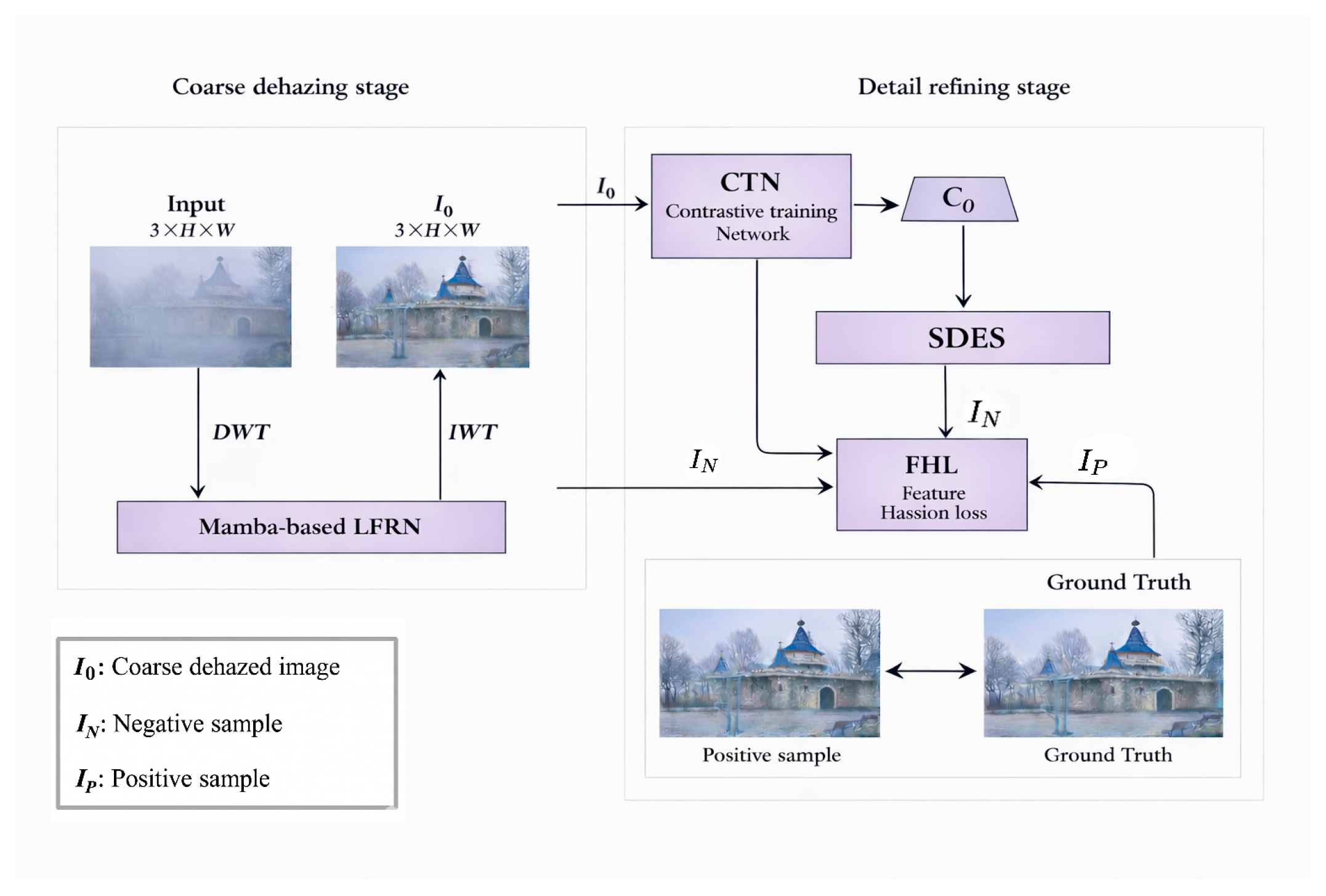
Our CoFiWaveMamba adopts a coarse-to-fine hazy image restoration scheme, including a low-frequency restoration stage and two progressive high-frequency tuning stages.

First, the low-frequency restoration network (LFRN) processes only the low-frequency component $I_{LL}$ to recover the global haze veil and illumination, producing

$${\widehat{I}}_{LL}=f_{LF}(I_{LL}).$$

(9)

Unlike conventional single-path low-frequency backbones, the proposed LFRN incorporates a dual-branch Spatial State Space Block:

(i)

A selective-scan state space branch to model long-range dependencies and global structures;

(ii)

An Efficient Spatial Context Mixer (ESCM) branch that captures local spatial interactions with a large receptive field.

The two branches are adaptively fused via a gating mechanism, improving representation capacity with low computational overhead. We then combine ${\widehat{I}}_{LL}$ with the original high-frequency components to obtain a coarse restoration:

$$X_1=\lambda X+DP\left(SS2D(\widehat{X})\right)$$

(10)

$$X_2=\lambda X+DP\left(SiLU(\widehat{X})\odot LSM(Con{v}_{1\times 1}(\widehat{X}))\right)$$

(11)

$$Y=\lambda \widehat{X}+DP(Linear([X_1 ;X_2 ]))$$

(12)

We formulate high-frequency restoration as a two-stage coarse-to-fine tuning process. Specifically, progressive high-frequency refinement is realized by two cascaded tuning networks. We first design a coarse-tuning network (CTN) for coarse high-frequency recovery, where a lightweight CNN-based refinement module quickly mitigates prominent texture loss and edge blurring in the LFRN output. This provides a cleaner initialization for the subsequent fine-tuning network (FTN) to perform fine-grained refinement. The specific details of each component are shown in Figure 1.

2.3.1. Spatially Modulated Low-Frequency Restoration Network (SM-LFRN)

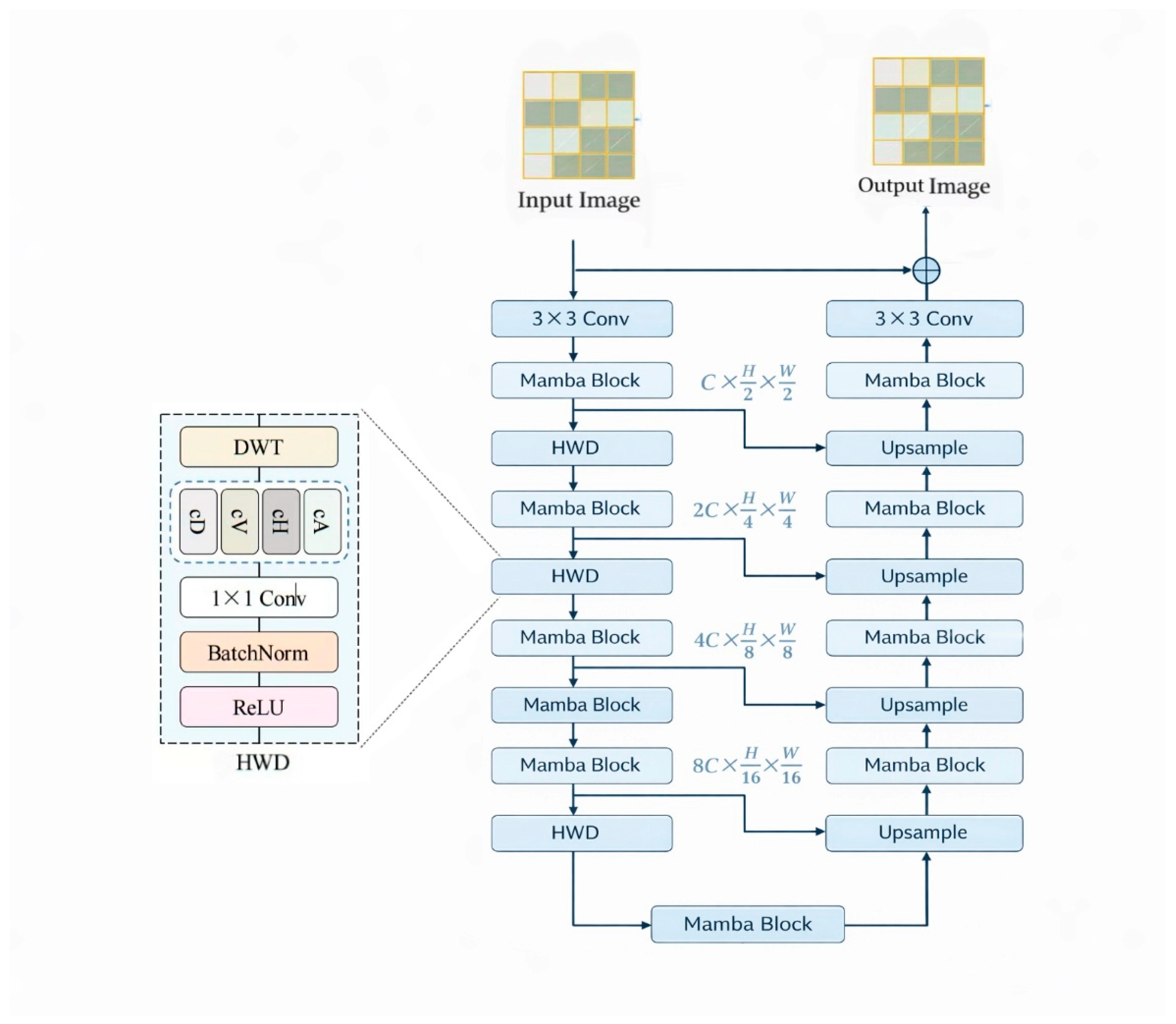
SM-LFRN is used to restore the low-frequency component $A_{low}$. Its structure is built on a U-shaped backbone. We use an improved Mamba block. It allows the network to model low-frequency information over a larger range and also helps preserve the overall scene structure and brightness distribution. In addition, wavelet downsampling [36] is used instead of conventional downsampling to avoid the loss of spatial information and reduce computational cost. This design is also naturally compatible with the long-range modeling ability of Mamba.

Haar Wavelet Downsampling: In image restoration, downsampling is commonly performed with strided convolutions to aggregate local features and expand the receptive field. However, this approach can result in the loss of crucial spatial details. As an alternative, Haar wavelet downsampling (HWD) [36] has recently gained attention, showing superior performance in tasks such as semantic segmentation. Motivated by this, we adopt HWD in our low-frequency restoration network to better retain important information.

The HWD process, shown in Figure 2, begins by applying the Haar wavelet transform to the input features, generating four subbands, each with half the spatial resolution of the original input. These subbands are then concatenated along the channel dimension. A 1 × 1 convolution is applied afterward to facilitate cross-channel interaction, followed by batch normalization and ReLU activation. By combining reduced spatial resolution with the information-preserving properties of the Haar transform, HWD allows downsampling with minimal information loss, thereby improving the network’s dehazing capability.

Mamba Block: As shown in Figure 3, the input features first pass through the first LayerNorm and are then fed into the SM-SSM branch for global context modeling. The output of the SM-SSM branch is added to the input through a residual connection, and the result is then sent to the following feed-forward network (FFN). The entire process can be expressed as follows:

$$F_{h }=SMSSM(LN(F_A^{in} )+\alpha \cdot F_{A }^{in}$$

(13)

$$F_{A }^{out}=FFN(LN(F_{h }))+\beta \cdot F_h$$

(14)

where $F_{h }$ denotes the intermediate hidden feature, $LN(\cdot )$ represents the layer normalization operation, $SMSSM(\cdot )$ and $FFN(\cdot )$ correspond to the SM-SSM and FFN mappings, respectively, and $\alpha$ and $\beta$ are learnable skip-scaling factors.

SM-SSM: The input of SM-SSM is processed by two branches and then fused for output. Branch 1 uses SS2D [21,22] selective scanning to capture long-range global dependencies and introduces SGSA to adaptively reweight the outputs from four directions, so as to achieve stable global trend recovery. Branch 2 uses a gated lightweight spatial context modulator (LiteSpatialMix) to provide structure-aware local compensation. The outputs of the two branches are first concatenated along the channel dimension and linearly fused, and then further refined through residual connections and an FFN, finally producing enhanced low-frequency features.

Given $X\in R^{B\times H\times W\times C}$, Branch 1 first applies LayerNorm and then uses a linear projection to produce a content stream and a gating stream. The content stream is injected with local spatial prior by depthwise convolution and then processed by SS2D with four directional selective scans, yielding four directional outputs. Since different scanning directions cover different contexts, direct summation aggregation can introduce fusion instability and limit complementarity.

We, therefore, insert SGSA [26] before aggregation: we concatenate four outputs along channels, perform shuffle → global pooling → grouped $1\times 1$ convolution → sigmoid to generate channel-wise, direction-wise weights, and finally “rearrange back” the weights to align directional channels. The reweighted directional outputs are then summed and projected back to $C$ channels with gated output modulation.

$$\tilde{X}=LN(X).$$

(15)

$$U_{k }=SSA\left({\mathrm{\Phi }}_{k }(\tilde{X})\right),\hspace{1em}k\in \left\{1,2,3,4\right\}.$$

(16)

$$Y=Cat(U_{1 },U_2 ,U_{3 },U_4 )\in R^{B\times H\times W\times 4C^{″}},A_{1:4} =SGSA([U_{1 };U_2 ;U_3 ;U_{4 }])$$

(17)

$$Branch1(X)=X\odot \alpha +DP(U)$$

(18)

where $B$, $H$, $W$, and $C$ denote the batch size, spatial size, and number of channels of the feature map, respectively, ${\mathrm{\Phi }}_{k }(\cdot )$ denotes the serialized operator for k scanning directions, $SSA$ denotes selective scan/state space update, $DP(\cdot )$ denotes stochastic depth, $\odot$ denotes channel-wise broadcast multiplication, and $[;]$ denotes concatenation along the channel dimension.

Spatial modulation branch: Branch 2 complements the limited local adaptivity of Branch 1 through gating and spatial context mixing. Specifically, the input $\tilde{X}$ is first processed by $SiLU$ to generate a spatial gate $G$, followed by a $1\times 1$ convolution for channel reorganization, and then fed into the lightweight spatial context modulator LSM (LiteSpatialMix). LSM applies large-kernel and dilated depthwise convolutions to the high-frequency features of the image to expand the receptive field. while the remaining channels are directly passed through to preserve feature fidelity. Channel shuffle and grouped $1\times 1$ convolutions are then used for low-cost full-channel mixing, and layer-scale is employed to suppress early training oscillations. The final output is modulated by the gate $G$, achieving spatially adaptive compensation that enhances structural regions while suppressing flat regions.

$$G=\delta (\tilde{X}),\hspace{1em}V=Con{v}_{1\times 1} (\tilde{X}),\hspace{1em}S=\mathrm{ESCM}(V)$$

(19)

$$Y_{2 }=X\odot \alpha +DP(G\odot S)$$

(20)

Convert $V$ to $BCWH$ format and split it along the channel dimension.

$$V=[V_p ,V_r ],V_p \in R^{B\times C_{p }\times H\times W}$$

(21)

Perform partial channel-spatial mixing on $Vp$, and apply lightweight channel attention ECA [37] to $T$.

$$T=\delta \left(DWCon{v}_{3\times 3} (Vp )+DWCon{v}_{k\times k}^{(d) } (V_{p })\right)$$

(22)

$$w=\sigma \left(Conv1D(GAP(T))\right),\hspace{1em}\widehat{T}=T\odot w$$

(23)

where $\delta$ denotes $SiLU$, $\sigma$ is $Sigmoid$, and $GAP$ denotes global average pooling.

Finally, concatenate $\widehat{T}$ and $V_r$, perform the shuffle operation, and finally mix them with grouped 1 × 1 convolutions.

$$\widehat{V}=PWCon{v}_{1\times 1}\left(Shuffle([T,V_r])\right),\hspace{1em}ESCM(V)=\gamma \cdot \widehat{V}$$

(24)

where $\gamma$ denotes layer-scale.

With $Y_1$ and $Y_2$, we concatenate them along channels and linearly project back to $C$ channels for cross-branch information exchange and complementary fusion.

$$F=Linear(Cat(Y_1 ,Y_{2 })),Z=X\odot \alpha +DP(F),$$

(25)

$$LFSSBlock(X)=Z\odot \beta +FFN(LN(Z))$$

(26)

where $\alpha$ and $\beta$ are learnable skip-scale parameters, Linear denotes the linear projection that maps 2C to C, $FFN(\cdot )$ denotes the lightweight gated feed-forward network, and $\beta$ acts as the residual scaling factor in the second branch.

2.3.2. Coarse-Tuning Network

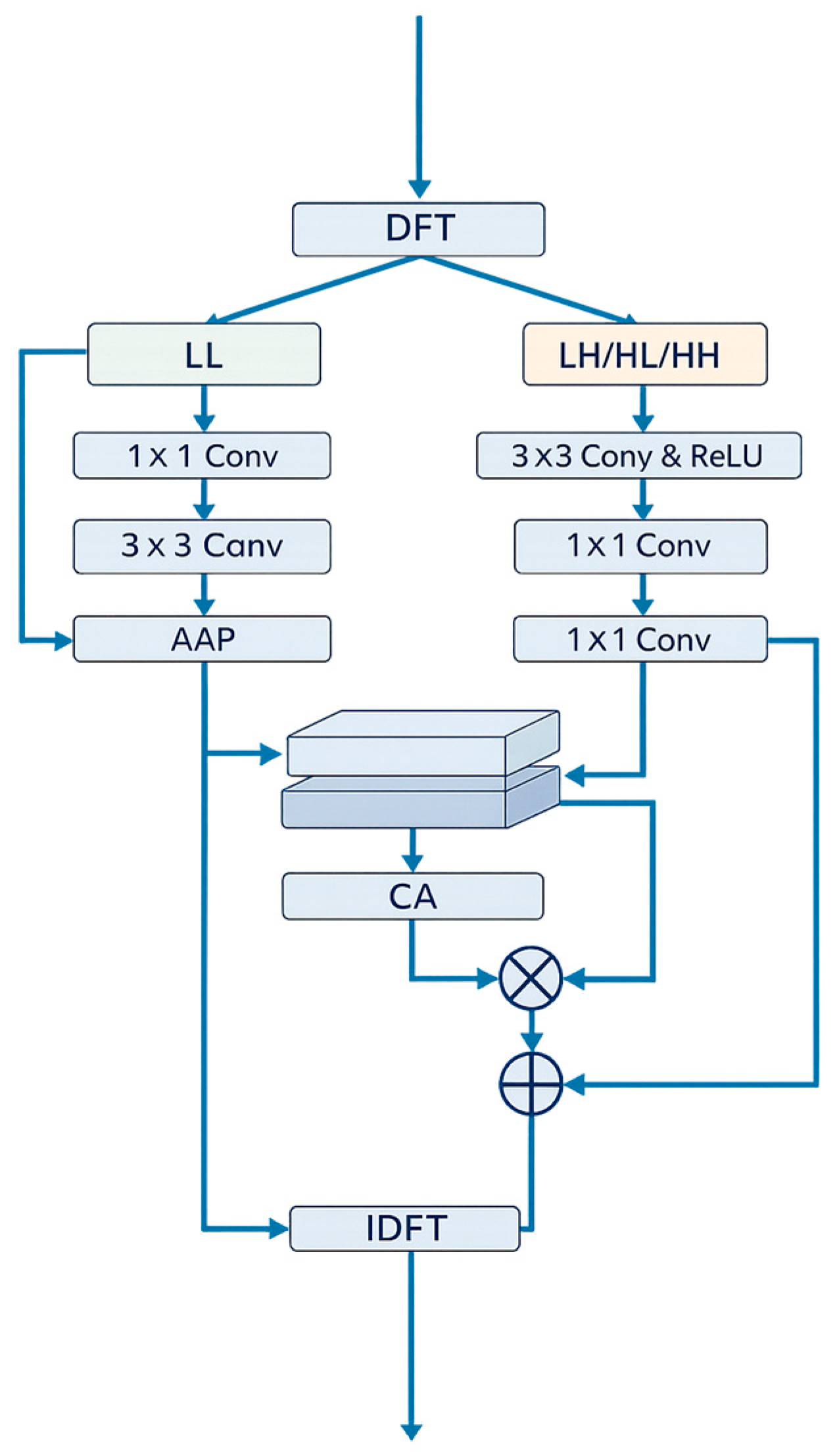
As shown in Figure 4, the coarse-tuning network decomposes the input into low- and high-frequency subbands, enhances each to preserve structure and details, and then fuses them via a gating mechanism, thereby achieving preliminary restoration of the image’s overall structure, brightness distribution, and edge details, providing a reliable foundation for subsequent fine-grained restoration.

For the input feature $X$, a discrete wavelet transform is first applied to decompose it into one low-frequency subband $LL$ and three high-frequency subbands $LH$, $HL$, and $HH$:

$$DWT(X)=[LL,LH,HL,HH]$$

(27)

The three high-frequency subbands are then concatenated as follows:

$$H=[LH,HL,HH]$$

(28)

A low-frequency guidance mapping ${\varphi }_{l }(\cdot )$ is applied to $LL$. Specifically, $LL$ is first processed by a $1\times 1$ convolution followed by a $3\times 3$ depthwise convolution to obtain $Z_l$, which aligns the low-frequency features to a suitable dimension for subsequent fusion while capturing smooth structures, illumination trends, and large-scale residual haze.

Then, after ASSM modulation is applied to $Z_l$, average pooling, a $1\times 1$ convolution, and a nonlinear activation are applied to $Z_l$ to emphasize low-frequency structural information beneficial for restoration and suppress ineffective low-frequency responses. In Figure 4, it is the operation of AAP. The formulation is given by

$$Z_l =DWCon{v}_{3\times 3 }(Con{v}_{1\times 1 }(LL)),{\varphi }_{l }(LL)=\sigma (Con{v}_{1\times 1 }(GAP(Z_{l })))\odot Z_l$$

(29)

Here, $Con{v}_{1\times 1 }$ is used for channel alignment and compression, $Con{v}_{3\times 3 }$ is employed to extract local structural context in the low-frequency space, and $GAP(\cdot )$ denotes global average pooling, which is used to generate a global channel descriptor. Finally, sigmoid is adopted to produce channel-wise weights for lightweight recalibration of the low-frequency features.

H is processed by the high-frequency enhancement mapping ${\psi }_{h }(\cdot )$, which compensates for the edges, textures, and directional details contained in the high-frequency subbands $LH,HL,HH$, while avoiding the ringing artifacts and false edges that may result from direct uniform amplification. Since the three high-frequency subbands correspond to different directional information, a more reasonable strategy is to model them separately before fusion. Specifically, each subband is first processed by a $3\times 3$ depthwise convolution, followed by a nonlinear activation and a $1\times 1$ convolution, to extract local high-frequency patterns and perform channel mixing. The enhanced responses from the three directions are then concatenated and fused to form a unified high-frequency compensation representation. The detailed formulation is given as follows:

$$E_i =Con{v}_{1\times 1 }(\delta (DWCon{v}_{3\times 3 }(Hi ))),i\in \{LH,HL,HH\}$$

(30)

$${\psi }_{h }(H)=Con{v}_{1\times 1} ([E_{LH} ,E_{HL} ,E_{HH} ])$$

(31)

where $\delta (\cdot )$ denotes $SiLU$.

Then, the low-frequency context and high-frequency responses are jointly used to generate a gating map $M$, which is further employed to modulate the enhancement strength of the high-frequency components:

$$M=\delta (Con{v}_{1\times 1}([{\varphi }_l(LL),{\psi }_h(H)])),\widehat{H}=H+M\odot {\psi }_h(H)$$

(32)

Here, $\psi (\cdot )$ denotes a lightweight high-frequency enhancement mapping used to extract and compensate high-frequency details; $\varphi (\cdot )$ denotes a low-frequency guidance mapping that provides global structural and illumination priors; $\delta (\cdot )$ is the sigmoid function; and $M\in [0,1]$ represents position-aware and channel-aware enhancement weights. Rather than uniformly amplifying all high-frequency responses, this design applies stronger enhancement only to edge and texture regions while maintaining suppression in noisy or artifact-prone regions, thereby effectively alleviating over-sharpening and ringing artifacts.

For the low-frequency subband, instead of performing strong enhancement, we adopt a lightweight correction strategy:

$$\tilde{L}=LL+\beta \cdot {\varphi }_l (LL)$$

(33)

where $\beta$ is a learnable scaling factor. The reason for this design is that the low-frequency component mainly carries the overall structure, brightness, and color distribution of the image. Directly applying strong enhancement to it may easily lead to color shifting, structural distortion, and amplification of residual haze. Finally, the output of the frequency-domain branch is reconstructed by the inverse wavelet transform:

$$F=IDWT(LL,LH,HL,HH)$$

(34)

2.3.3. Fine-Tuning Network

The fine-tuning network aims to further restore delicate high-frequency textures and suppress residual artifacts such as a slight haze veil, ringing, and detail loss caused by over-smoothing after the coarse restoration.

A key challenge in this stage is that local detail enhancement alone is prone to unstable amplification: once the coarse restoration still contains residual haze bias or slight structural deviation, directly sharpening directional subbands may generate visually sharp but globally inconsistent textures. To alleviate this issue, we combine Fourier-domain and wavelet-domain modeling in a complementary manner. The Fourier representation constrains the global distribution of high-frequency responses, while the wavelet representation preserves spatial localization and directional sensitivity. In this way, global spectral regularity is used to guide local directional reconstruction, reducing ringing and pseudo-detail amplification.

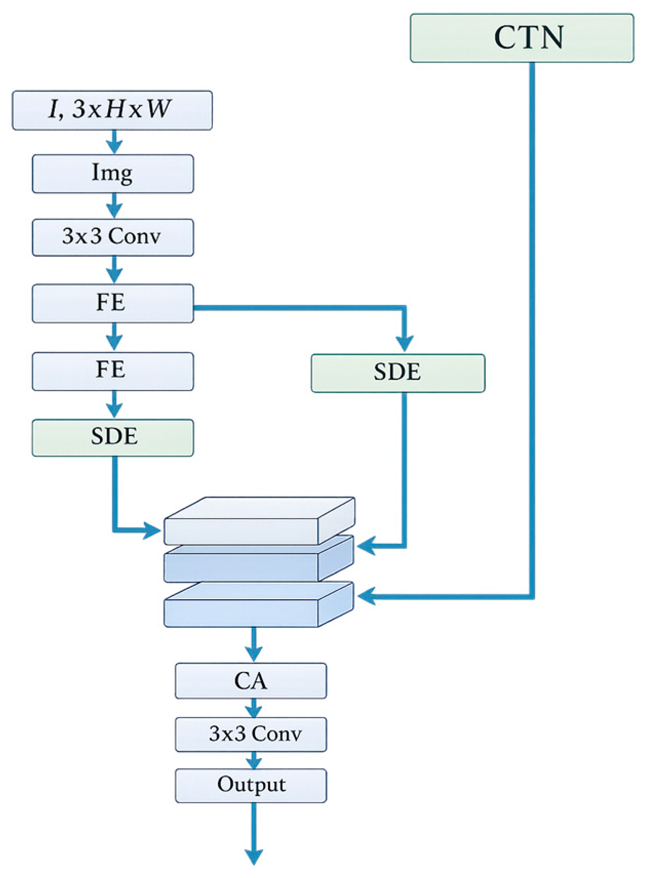
As shown in Figure 5, for the coarsely restored image produced by low-frequency restoration, we first perform deeper feature extraction and stable local enhancement through cascaded grouped structures (FE), and then employ a wavelet-guided, subband-split frequency enhancement module (SDE) to explicitly restore directional textures, instead of implicitly mixing information from different directions. Given the CTN output $\widehat{I}\in R^{3\times H\times W}$, FTN performs residual learning:

$$\widehat{I}=I^{(1)}+f_{FTN}(I^{(1)}).$$

(35)

Here, $f_{FTN}(\cdot )$ denotes the nonlinear mapping of FTN, and $\widehat{I}$ is the final output.

Feature Extraction Module (FE): FTN first applies a $3\times 3$ convolution to extract shallow features. Then two cascaded FE are used, where each FE stacks multiple blocks, followed by an extra convolution and a group-level skip connection. Each block follows a “conv → activation → residual → conv → U-Block → residual” pattern, enabling lightweight U-shaped multi-scale fusion and stable training.

Subband Detail Enhancement Net: A Subband Detail Enhancement Net (SDE) is inserted after each Feature Extraction Module. The first SDE emphasizes stability, while the second SDE activates a stronger ASSM on magnitude [21] to capture longer-range frequency correlations. This forms a “weak-to-strong” progressive tuning: early refinement avoids destabilizing global updates, while later refinement releases stronger modeling capacity for higher detail fidelity.

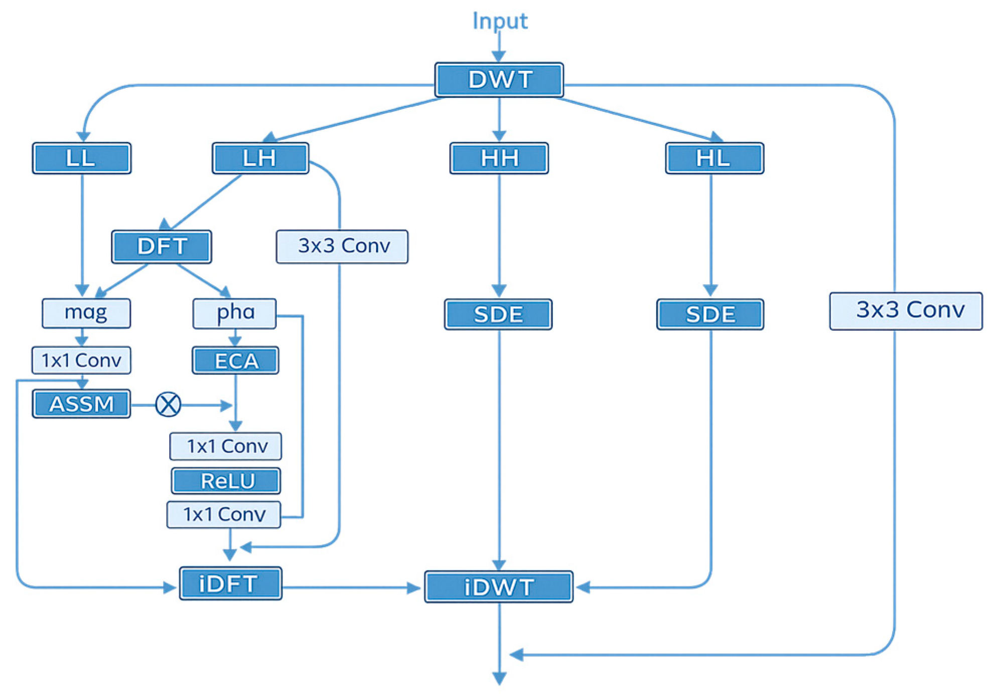
As shown in Figure 6, the Subband Detail Enhancement Net (SDE) does not directly perform detail restoration on the full feature map, but instead adopts a subband frequency enhancement strategy: it first performs wavelet decomposition [23,24], then separately enhances the three directional high-frequency subbands, while using the low-frequency magnitude as structural guidance.

$$\{F_{LL} ,F_{HL },F_{LH },F_{HH} \}=DWT(F).$$

(36)

Here, $F\in R^{C\times H\times W}$ is the input feature; $F_{LL}\in R^{C\times {\displaystyle \frac{H}{2}}\times {\displaystyle \frac{W}{2}}}$ is the low-frequency subband; $F_{HL },F_{LH },F_{HH}$ correspond to horizontal, vertical, and diagonal textures, respectively.

For each directional subband, we introduce Fourier-domain modulation not to replace spatially localized restoration, but to regularize it. The amplitude spectrum characterizes the global strength distribution of frequency components and is thus used to stabilize how strongly different high-frequency responses should be enhanced. The phase spectrum is closely related to structural arrangement and edge localization; therefore, phase refinement under amplitude guidance helps preserve edge positions while avoiding structurally inconsistent sharpening.

For a given feature $F_n$, four subbands are first obtained through wavelet decomposition. For each directional subband, the FFT is applied to extract the amplitude A and phase P of the high-frequency subband. Then, following the method in the UVM-Net paper, the amplitude is enhanced by ASSM. ASSM is applied to the amplitude branch to capture long-range correlations in the global spectral distribution, so that the enhancement strength of directional details is globally regularized rather than determined only by local responses. The phase branch is then refined with ECA under the guidance of the enhanced amplitude, because phase is more sensitive to structural arrangement and edge positioning. This design allows the model to preserve spatially meaningful detail locations while avoiding unstable amplification of high-frequency noise, which can be expressed as follows:

$$A\prime =PConv(A)$$

(37)

For the phase spectrum, the ECA mechanism is employed to adaptively model the inter-channel relationships, and the phase is further optimized under the guidance of the amplitude. Finally, a convolution operation is used for additional refinement. The formulation is as follows:

$$w_{A\prime }=Softmax(ASSM(A\prime ))$$

(38)

$$P^{\prime }=PConv(ReLU(PConv(({\omega }_{A^{\prime }}\cdot ECA(P)))))+P$$

(39)

where denotes $AAP(\cdot )$ adaptive average pooling, and ${\omega }_{A^{\prime }}$ represents the attention weights of the enhanced amplitude spectrum. Finally, the frequency-domain features are transformed back into the spatial domain via the inverse Fourier transform.

After detail reconstruction is completed for each subband, the feature map is reconstructed through the inverse wavelet transform:

$$F\prime =IWT(F_{LL},{\widehat{F}}_{HL},{\widehat{F}}_{LH},{\widehat{F}}_{HH})$$

(40)

where $IWT(\cdot )$ denotes inverse wavelet transform for spatial-domain reconstruction.

Finally, SDE fuses a spatial $3\times 3$ convolution branch with the wavelet-frequency reconstructed branch in a residual manner to preserve locality while injecting frequency-corrected details.

Notably, to balance the number of parameters and prevent model overfitting, we apply ASSM-guided channel modeling in only one SDE, while the other SDE still uses 1 × 1 convolution and pooling operations to generate channel attention.

2.3.4. Self-Guided Contrastive Regularization (SGCR)

In image dehazing, we take the clear image $J$ (ground truth) and the hazy image $I$ as the positive sample and negative sample, respectively. The objective of contrastive regularization $R_{t }$ is to maximize the $L_1$ distance between the anchor and the negative sample in the feature space while minimizing the $L_1$ distance between the anchor and the positive sample. Its expression can be written as follows:

$$R_{t }={\displaystyle \sum _{i=1}^n{\omega }_{i }\frac{\parallel V_{i }(J)-V_{i }(f(I,\theta )){\parallel }_1}{\parallel V_{i }(I)-V_{i }(f(I,\theta )){\parallel }_1}}$$

(41)

where $f(\cdot ,\theta )$ denotes the parameterized dehazing network, and $V(\cdot )(i=1,2,\dots ,n)$ denotes the i-th latent feature extracted by the pre-trained VGG-19 [38] network, and ${\omega }_{i }$ denotes the corresponding weight. However, as the anchor gradually moves away from the negative sample and gets closer to the positive sample, the ability of the model to distinguish the dehazed image from the hazy input continues to increase. As a result, the influence of the hazy image gradually weakens, thereby limiting its effect in further improving the performance of the model. To alleviate this problem and promote the generation of more natural dehazing results, we introduce contrastive regularization in the WDMamba [24] paper. While treating the coarse restored image ${\widehat{I}}_0$ generated by the low-frequency restoration network as a hard negative sample, we also add the coarse restored image generated by CTN into the learning of hard negative samples. This design can better use the intermediate outputs of the model itself and guide the final prediction to better approximate the ground truth. The regularization term can be formally defined as follows:

$$R_{SG}={\displaystyle \sum _{i=1}^n{\omega }_{i }\frac{\parallel V_{i }(J)-V_{i }(f(I,\theta )){\parallel }_1}{\parallel V_{i }({\widehat{I}}_0)-V_{i }(f(I,\theta )){\parallel }_1+\parallel V_{i }({\widehat{I}}_{CNT})-V_{i }(f(I,\theta )){\parallel }_1}}$$

(42)

where ${\widehat{I}}_0$ denotes the coarse restored image generated by the low-frequency restoration network, and ${\widehat{I}}_{CNT}$ denotes the coarse restored image generated by CTN.

3. Experiments

In this section, we first introduce the experimental setup. We then verify the effectiveness of the proposed method through extensive experiments on various datasets. Finally, we conduct a detailed ablation analysis to validate our method.

3.1. Datasets and Task Setup

3.1.1. Datasets

For a comprehensive evaluation of the proposed CoFiWaveMamba model, we conduct quantitative and qualitative assessments on three synthetic dehazing datasets—Haze4K, RESIDE-6K, and HSTS-SYNTHETIC [8] (a hybrid subjective test set)—as well as one real-world paired hazy dataset, O-HAZE [39].

Specifically, Haze4K [40] and RESIDE-6K [8] are used as the main supervised training and quantitative evaluation datasets, since both provide paired hazy/clear images and have been widely adopted in recent dehazing studies. RESIDE-6K contains 6000 training images and 1000 test images. Haze4K contains 3000 training images and 1000 test images. The test sets of both datasets consist of a mixture of indoor and outdoor hazy images. The HSTS-SYNTHETIC synthetic dataset is composed of 10 test images without any training samples. In this work, the model trained on RESIDE-6K is used to evaluate performance on the HSTS-SYNTHETIC dataset.

O-HAZE [39] provides 45 real-world outdoor hazy images that are manually generated. The first 40 images are used for training and the remaining 5 for testing. This dataset is used to verify the practical robustness of the proposed method in real outdoor scenarios. All O-HAZE images are resized to a resolution of 1600 × 1200 pixels for evaluation. In addition, we have also supplemented cross-dataset generalization tests of the model on real-world datasets, including I-Haze, NH-Haze, and Dense-Haze, as well as synthetic datasets such as SOTS outdoor and HSTS-SYNTHETIC-Synthetic.

3.1.2. Implementation and Hardware Environment

Our model is implemented in PyTorch 2.2.2 and trained on a single NVIDIA RTX 4090 GPU. Unless otherwise specified, the random seed is fixed to 666 for reproducibility.

For the low-frequency restoration backbone, we adopt a WaveMamba architecture [41] with input channel number 3, base width 16, and multi-scale Mamba block configuration n_l_blocks = [1, 2, 2, 4, 4, 2, 2, 1]. In the high-frequency refinement stage (FTN), the feed-forward expansion ratio is set to 2.0. The fine-tuning network adopts three group (gsp) modules, each consisting of a feature extraction unit (FE) and a Subband Detail Enhancement Net (SDE). The specific connection is illustrated in Figure 5. The FE contains 6 residual blocks, denoted as FTNet (3, 6).

In real-image dehazing experiments, due to the limited number of training images, after a trade-off, we set the number of gps to 2 and the number of residual blocks in each FE to 4, i.e., FTNet(2, 4).

For optimization, we use AdamW for the generator with parameters

$${\beta }_{1 }=0.9,{\beta }_{2 }=0.99$$

(43)

We also use an initial learning rate of $5\times {10}^{-4},$ and a weight decay of $1\times {10}^{-3}$. The learning rate is gradually decayed to $1\times {10}^{-7}$.

Using a cosine annealing schedule. During training, we employ a combined objective consisting of L1 loss, SSIM loss (weight 0.25), and FFT loss (weight 0.1). Validation is performed every 5000 iterations, and the best model is selected according to PSNR.

For synthetic paired training, random paired cropping and geometric augmentation are used. On RESIDE-6K, we adopt a progressive training strategy to better balance convergence stability and high-resolution detail recovery.

In the first stage, the model is trained using 256 × 256 patches with a relatively larger batch size.

In the second stage, the patch size is increased to 400 × 400 while the batch size is reduced to improve fine-detail reconstruction.

In the final training configuration, the RESIDE-6K model is trained for a total of 500,000 iterations. The first stage reaches its upper limit at around 248,000 iterations, after which we switch to the second stage for fine-tuning.

For Haze4K, the model is trained with the same optimizer and scheduler settings, using paired supervision on the corresponding training split. For O-HAZE [39], due to the larger spatial resolution and higher memory consumption, we set the training patch size to 640 × 640 and the batch size to 2, with a total of 300,000 iterations.

We further conduct cross-dataset generalization tests on the lightweight variant CoFiWaveMamba-lite and the full CoFiWaveMamba model across synthetic datasets (SOTS outdoor and HSTS-SYNTHETIC-Synthetic) and real-world datasets, including I-Haze, NH-Haze, and Dense-Haze.

Table 1. Architectural differences between CoFiWaveMamba and CoFiWaveMamba-lite.

Component	CoFiWaveMamba (Full)	CoFiWaveMamba-Lite
Overall pipeline	LFRN → CTN → FTN	LFRN→ CTN-lite → FTN-lite
ffn_scale	2.0	1.5
CTN	Used	Used
CTN modulation	with ASSM-guided modulation	ASSM modulation removed
FTN groups (gps)	3	2
Blocks per Group	6	4
FTN ASSM hidden setting	d_state = 16, num_tokens = 64, inner_rank = 32, mlp_ratio = 2.0	d_state = 8, num_tokens = 32, inner_rank = 16, mlp_ratio = 1.5

summarizes the architectural differences between CoFiWaveMamba and its lightweight variant, CoFiWaveMamba-lite.

The core distinction lies in the CTN module: the full CoFiWaveMamba employs ASSM-guided modulation to enhance global frequency correlation modeling, while CoFiWaveMamba-lite removes this ASSM-based modulation structure and retains only lightweight global pooling operations. Additionally, the FTN of CoFiWaveMamba-lite is more lightweight than that of CoFiWaveMamba, featuring fewer groups and residual blocks.

3.1.3. Comparison Methods and Evaluation Metrics

We compare the proposed CoFiWaveMamba with two representative early dehazing methods, including DCP [4] and AOD-Net [14], as well as eleven recent state-of-the-art methods, namely, WDMamba [24], GDN [42], FFA-Net [16], Dehamer [17], DehazeFormer [18], IR-SDE [19], FSNet [43], PNE-Net [44], DEA-Net [15], OKNet [45], and ConvIR [46].

For quantitative evaluation on paired benchmarks, we use PSNR and SSIM as the primary full-reference metrics. Following the implementation setting in our codebase, evaluation on synthetic datasets is conducted with a 4-pixel border crop and Y-channel measurement [8,24], while evaluation on real paired benchmarks, such as O-HAZE [39], is performed in the RGB space.

3.2. Results

3.2.1. Comparison of Synthetic Dehazing Methods

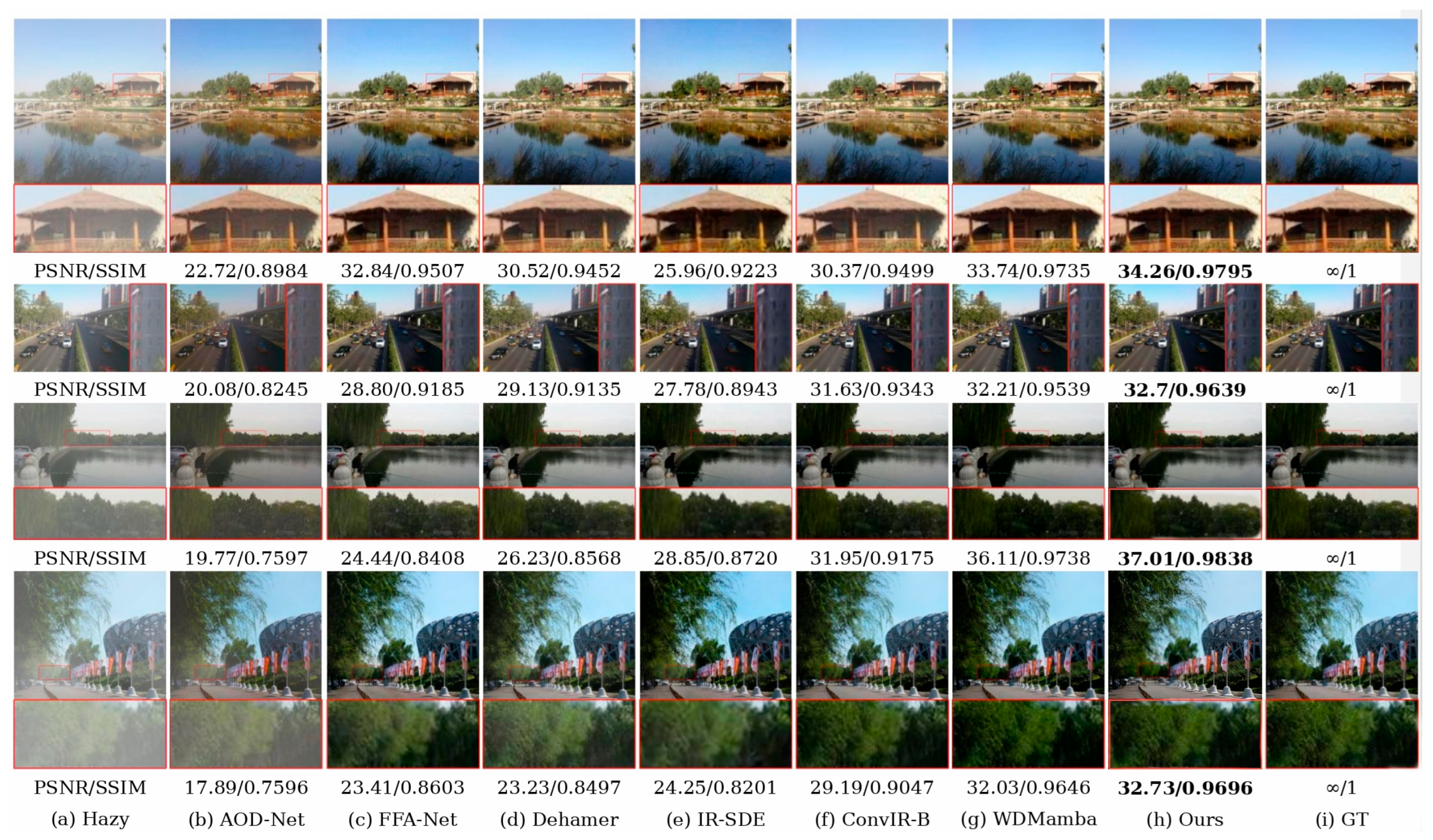
As can be seen from

Table 2. Quantitative comparison between our CoFiWaveMamba and 14 state-of-the-art dehazing methods on Haze4K, RESIDE-6K, HSTS-SYNTHETIC-SYNTHETIC, and O-HAZE. We report PSNR, SSIM, parameters, and FLOPs. Results in bold denote the best performance. while lower Params and FLOPs indicate lower model complexity. The best result in each column is shown in bold.

Method	Haze4K		RESIDE-6K		HSTS-SYNTHETIC		O-HAZE		Params (M)	FLOPs (G)
	PSNR	SSIM	PSNR	SSIM	PSNR	SSIM	PSNR	SSIM
DCP [4]	16.93	0.5877	17.88	0.8160	17.01	0.8030	14.65	0.6358	-	-
AOD-Net [14]	17.90	0.5946	19.88	0.8454	20.87	0.8411	18.19	0.6823	0.002	0.12
GDN [42]	25.72	0.9641	27.16	0.9544	29.71	0.9617	20.05	0.7362	0.96	21.55
FFA-Net [16]	28.21	0.9669	28.69	0.9577	28.82	0.9133	23.34	0.8084	4.46	287.8
Dehamer [17]	26.03	0.9392	28.12	0.9521	29.58	0.9207	24.36	0.8089	132.45	59.31
DehazeFormer-L [18]	31.86	0.9783	31.57	0.9696	34.08	0.9743	25.25	0.8206	25.45	277.02
IR-SDE [19]	29.57	0.9744	28.50	0.9575	27.60	0.8900	23.99	0.7652	135.3	119.1
FSNet [43]	34.09	0.9881	30.69	0.9672	30.54	0.9293	24.55	0.8483	13.28	110.5
PNE-Net [44]	31.07	0.9821	29.64	0.9635	28.81	0.9523	24.12	0.8354	4.76	308.31
DEA-Net [15]	34.22	0.9879	30.77	0.9681	31.66	0.9342	25.54	0.8196	3.65	32.23
OKNet [45]	32.42	0.9863	30.21	0.9613	31.39	0.9316	25.62	0.8528	14.3	39.71
ConvIR-B [46]	34.12	0.9877	30.96	0.9656	31.80	0.9347	26.09	0.8552	8.63	71.22
ConvIR-L [46]	34.50	0.9886	30.23	0.9504	31.82	0.9330	25.31	0.8511	14.83	129.34
WDMamba [24]	35.88	0.9909	32.15	0.9723	34.53	0.9739	27.22	0.8729	11.25	38.84
CoFiWaveMamba	35.93	0.9911	32.09	0.9801	35.40	0.9865	27.31	0.8731	12.36	39.61

, CoFiWaveMamba achieves highly competitive results. On Haze4K, it attains a PSNR of 35.93 dB and an SSIM of 0.9911, achieving the best PSNR and SSIM. On the RESIDE-6K dataset, although its PSNR is slightly lower than that of WDMamba, CoFiWaveMamba achieves a significantly higher SSIM of 0.9801, indicating better structural preservation. In addition, on the HSTS-SYNTHETIC dataset, CoFiWaveMamba achieves the best peak signal-to-noise ratio (PSNR) and the best structural similarity index (SSIM). These comprehensive quantitative analyses demonstrate that our CoFiWaveMamba delivers superior dehazing performance. As shown in Figure 7, the clarity of the images restored by our method is very close to that of the ground truth, and its visual performance is consistently better than that of other models. In particular, even in distant regions, where dehazing is generally more challenging, our method is still able to remove haze effectively.

3.2.2. Real-World Hazy Image Evaluation

To further assess the practical robustness of the proposed method, we first report its performance on the paired real-world O-HAZE benchmark. As shown in Table 2, CoFiWaveMamba achieves 27.31 dB PSNR and 0.8731 SSIM, outperforming WDMamba. This result demonstrates that the proposed framework remains effective when both training and evaluation are conducted on real hazy images.

To further evaluate cross-dataset generalization, we additionally test the models trained on RESIDE-6K and Haze4K on unseen synthetic and real-world datasets, including HSTS-SYNTHETIC, SOTS outdoor, I-Haze, NH-Haze, and Dense-Haze, as reported in

Table 3. Quantitative cross-dataset evaluation of different methods on unseen synthetic and real-world hazy benchmarks, where all models are trained on RESIDE-6K and directly tested on HSTS-SYNTHETIC-Synthetic, SOTS outdoor, I-Haze, NH-Haze, and Dense-Haze. Bold indicates the best result in each column. Higher PSNR and SSIM values indicate better performance. Bold values indicate the results where our method outperforms WDMamba in the corresponding column.

Model	HSTS-SYNTHETIC PSNR/SSIM	SOTS Outdoor PSNR/SSIM	I-Haze PSNR/SSIM	NH-Haze PSNR/SSIM	Dense-Haze PSNR/SSIM
WDMamba	34.0057/0.9826	33.2443/0.9811	16.1998/0.7572	12.4008/0.4732	10.7073/0.4232
CoFiWaveMamba-lite	34.6600/0.9837	33.479/0.9813	16.4182/0.7622	12.2496/0.4661	11.1100/0.4292
CoFiWaveMamba	35.4013/0.9865	33.9693/0.9825	16.9160/0.7822	12.2496/0.4661	11.3100/0.4362

and

Table 4. Quantitative cross-dataset evaluation of different methods on unseen synthetic and real-world hazy benchmarks, where all models are trained on Haze4K and directly tested on HSTS-SYNTHETIC-Synthetic, SOTS outdoor, I-Haze, NH-Haze, and Dense-Haze. Bold indicates the best result in each column. Higher PSNR and SSIM values indicate better performance. Bold values indicate the results where our method outperforms WDMamba in the corresponding column.

Model	HSTS-SYNTHETIC PSNR/SSIM	SOTS Outdoor PSNR/SSIM	I-Haze PSNR/SSIM	NH-Haze PSNR/SSIM	Dense-Haze PSNR/SSIM
WDMamba	27.4586/0.9616	27.0562/0.9631	17.1581/0.7597	12.0310/0.5061	10.8070/0.42026
CoFiWaveMamba-lite	27.9869/0.9774	27.3528/0.9698	17.3814/0.7601	11.7998/0.5001	11.1800/0.42626
CoFiWaveMamba	28.6316/0.9828	27.9296/0.9763	18.0184/0.7876	12.1007/0.5066	11.4618/0.43162

. When trained on RESIDE-6K, CoFiWaveMamba achieves the best performance on HSTS-SYNTHETIC, SOTS outdoor, I-Haze, and Dense-Haze, while remaining competitive on NH-Haze. When trained on Haze4K, CoFiWaveMamba consistently outperforms WDMamba on all five target datasets. These results indicate that the proposed method is less sensitive to distribution shift and exhibits stronger cross-dataset generalization ability.

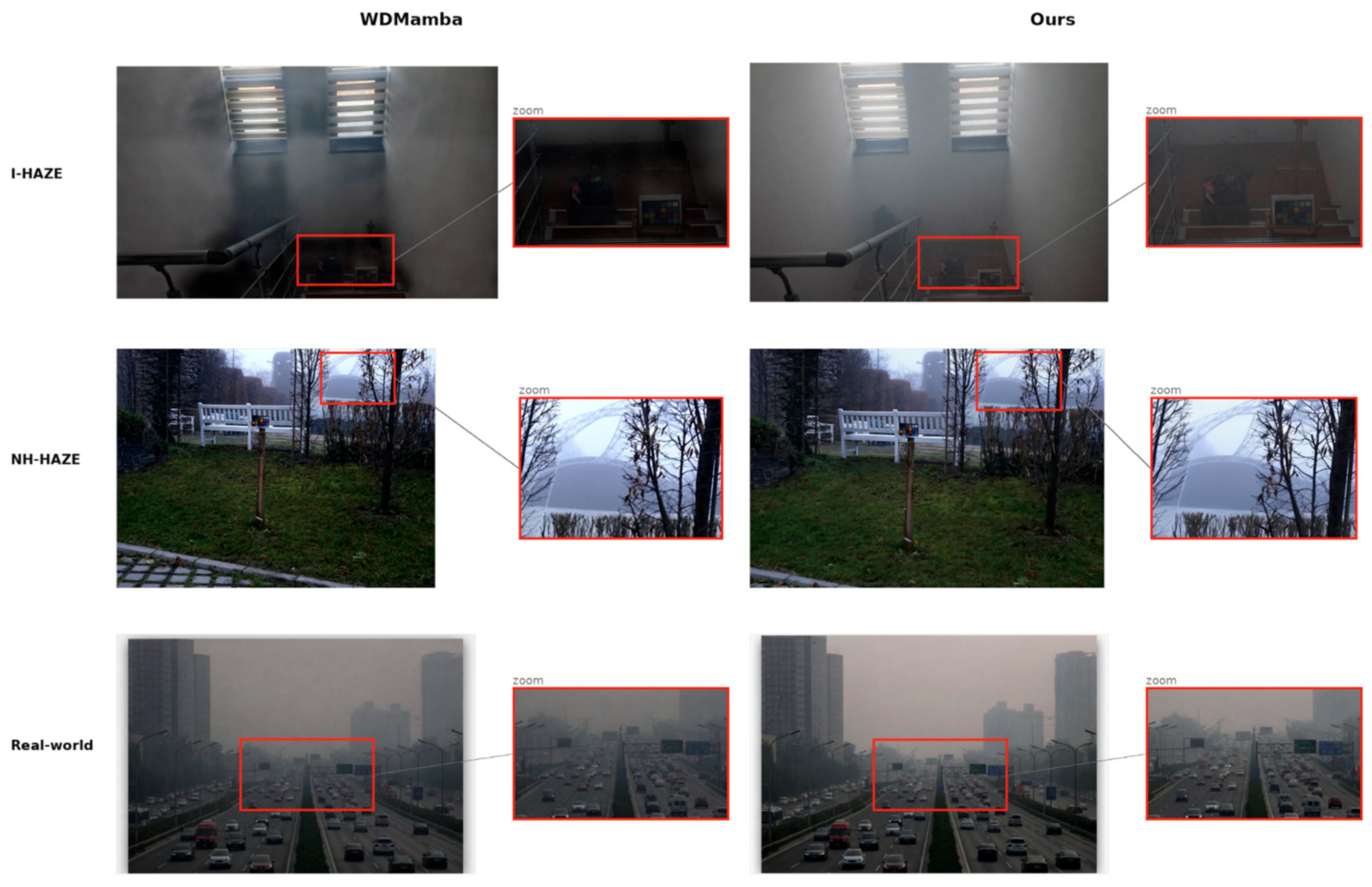
The visual comparisons in Figure 8 further support the quantitative results. Compared with WDMamba, CoFiWaveMamba restores clearer contours, better local visibility, and more distinguishable details in challenging hazy regions. Overall, these results demonstrate that the proposed high–low frequency collaborative design is effective not only for in-domain restoration, but also for improving robustness and transferability under real-world haze conditions.

The visual comparisons in Figure 8 further support the above quantitative observations. In the I-Haze and NH-Haze examples, CoFiWaveMamba recovers sharper and more faithful local structures than WDMamba, as evidenced by the enlarged regions, where object boundaries, fine textures, and small structural details are more clearly preserved. For the unpaired real-world hazy image collected from the Internet, although no-reference metrics are unavailable, our method still produces a visually cleaner result with better local visibility and more natural detail restoration, while introducing fewer oversmoothed or blurred regions. These observations are consistent with the proposed high–low frequency collaborative design: the low-frequency branch helps stabilize global haze removal and structural recovery, while the progressive high-frequency refinement further improves edge and texture reconstruction. Overall, the visual results demonstrate that CoFiWaveMamba is able to achieve more robust and transferable dehazing performance under real-world haze conditions.

3.3. Ablation Experiments

To better understand the contribution of each component, we conduct ablation experiments on the proposed model. As shown in

Table 5. Ablation study on CTN and FTN. √ indicates that the corresponding module is enabled, while × indicates that it is disabled. Higher PSNR and SSIM values indicate better performance.

Model	CTN	FTN	RESIDE-6K PSNR	RESIDE-6K SSIM	SOTS Outdoor PSNR	SOTS Outdoor SSIM
B1	×	×	29.68	0.9533	31.81	0.9433
B2	√	×	30.55	0.9687	32.31	0.9703
B3	×	√	31.78	0.9709	33.08	0.9789
B4	√	√	32.13	0.9782	33.97	0.9825

and

Table 6. Ablation study on SM-SSM and SGSA. √ indicates that the corresponding module is enabled, while × indicates that it is disabled. Higher PSNR and SSIM values indicate better performance.

Model	SM-SSM	SGSA	RESIDE-6K PSNR	RESIDE-6K SSIM
A1	×	×	32.01	0.9773
A2	√	×	32.06	0.9777
A3	×	√	32.08	0.9779
A4	√	√	32.13	0.9782

, both CTN and FTN help improve the dehazing performance, and the best results are achieved when the two modules are used together, which suggests that they play complementary roles in the restoration process. We also evaluate the effect of SM-SSM and SGSA in the low-frequency branch. Although each module brings only a modest improvement when used alone, combining them still leads to the best performance, showing that both are beneficial for enhancing feature representation. Overall, these results confirm that each proposed component contributes positively to the final performance of the network.

4. Discussion

The experimental results demonstrate that the proposed CoFiWaveMamba provides a balanced and effective solution for single image dehazing. Compared with existing methods, its advantage is not simply reflected in one specific benchmark, but in a more stable performance trend across synthetic, cross-dataset, and real-scene settings.

The proposed collaborative design between low- and high-frequency components in this work contributes to improved model generalization. Existing wavelet-based dehazing frameworks typically decompose the restoration process into low-frequency structure recovery and high-frequency detail enhancement. While this improves interpretability, it can also lead to an overly rigid restoration process in complex degradation scenarios. In contrast, CoFiWaveMamba emphasizes the collaborative interaction between global high-frequency-guided low-frequency restoration and progressively refined high-frequency reconstruction.

The superior performance on the HSTS-SYNTHETIC and O-HAZE datasets demonstrates that, when there exists a discrepancy between the haze distribution, image content, and degradation characteristics of the training and testing data, the proposed design enables the model to maintain stronger robustness.

This is because haze degradation is inherently cross-frequency coupled rather than independently distributed across frequency bands. In real-world scenarios, low-frequency components are closely related to the global haze veil, illumination shifts, and overall scene contrast, whereas high-frequency components are affected by edge diffusion, texture attenuation, and directional detail degradation. If these two components are restored in a strictly decoupled manner, biases introduced in the low-frequency stage may propagate into subsequent high-frequency reconstruction, leading to dataset-dependent artifacts such as over-sharpening, ringing effects, or structural inconsistencies in textures. Meanwhile, valuable high-frequency cues cannot be fully exploited.

In contrast, the proposed framework first stabilizes global low-frequency restoration through long-range dependency modeling, and then progressively refines high-frequency details in a coarse-to-fine manner. This strategy reduces error amplification across stages and makes the restoration process less sensitive to the specific statistical properties of haze in the training data, thereby improving cross-dataset robustness.

In this sense, the benefit of the proposed high–low frequency collaborative design is not only better frequency decomposition, but also a more stable restoration pathway. The low-frequency branch provides a more reliable global structural prior, while the progressive high-frequency branch avoids directly over-amplifying uncertain details. Their coordination helps preserve global consistency and local realism simultaneously, which is particularly important when the haze density, scene content, or illumination pattern differs from the training distribution.

From an efficiency perspective, the proposed framework keeps the overall complexity close to WDMamba in terms of parameters and FLOPs, while introducing only limited extra overhead through the progressive refinement stages. This is because the low-frequency branch performs most global modeling in a compact wavelet space, and the high-frequency branch refines directional details progressively rather than applying heavy global modeling to the full-resolution image. Nevertheless, runtime and memory consumption still increase with input resolution, especially in the fine-refinement stage, which should be further optimized in future lightweight designs.

Although the proposed method shows promising results, several limitations still remain. First, the current study mainly follows the standard supervised dehazing protocol based on paired training data. While cross-dataset testing and real-scene evaluation have been included to examine practical robustness, more diverse unpaired or weakly supervised settings are still worth further investigation. Second, the progressive design improves restoration quality, but it also introduces additional stages and modules, which may limit deployment efficiency in resource-constrained scenarios. Third, the present work focuses on image-level restoration quality and generalization, and its effect on downstream high-level vision tasks, such as detection or segmentation under haze, has not yet been systematically evaluated. These directions are important but go beyond the main scope of the current method-oriented study and will be explored in future work.

5. Conclusions

In this paper, we proposed CoFiWaveMamba, a coarse-to-fine wavelet-guided Mamba network for single image dehazing. The proposed method combines Mamba-based long-range dependency modeling in the low-frequency branch with progressive high-frequency refinement in the Fourier and wavelet domains, aiming to improve the coordination between global haze removal and local detail reconstruction. Experimental results on Haze4K, RESIDE-6K, HSTS-SYNTHETIC, SOTS, and O-HAZE show that CoFiWaveMamba achieves competitive overall performance and exhibits stronger robustness on cross-dataset and real-scene benchmarks. In addition, ablation studies verify that the proposed CTN, FTN, and SM-SSM modules all contribute positively to the final results. Overall, the proposed method demonstrates that a more coordinated high–low frequency collaborative strategy is beneficial for reducing residual haze, preserving structural consistency, and restoring finer textures in challenging dehazing scenarios.

References

1. Sakaridis, C.; Dai, D.; Van Gool, L. Semantic Foggy Scene Understanding with Synthetic Data. Int. J. Comput. Vis. 2018, 126, 973–992. [Google Scholar] [CrossRef]
2. Yang, X.; Mi, M.B.; Yuan, Y.; Wang, X.; Tan, R.T. Object Detection in Foggy Scenes by Embedding Depth and Reconstruction into Domain Adaptation. In Computer Vision—ACCV 2022; Springer: Cham, Switzerland, 2023; pp. 303–318. [Google Scholar]
3. Ren, W.; Zhang, J.; Xu, X.; Ma, L.; Cao, X.; Meng, G.; Liu, W. Deep Video Dehazing with Semantic Segmentation. IEEE Trans. Image Process. 2019, 28, 1895–1908. [Google Scholar] [CrossRef] [PubMed]
4. He, K.; Sun, J.; Tang, X. Single Image Haze Removal Using Dark Channel Prior. IEEE Trans. Pattern Anal. Mach. Intell. 2011, 33, 2341–2353. [Google Scholar] [PubMed]
5. Meng, G.; Wang, Y.; Duan, J.; Xiang, S.; Pan, C. Efficient image dehazing with boundary constraint and contextual regularization. In Proceedings of the IEEE International Conference on Computer Vision (ICCV), Sydney, Australia, 1–8 December 2013. [Google Scholar]
6. Berman, D.; Treibitz, T.; Avidan, S. Non-local Image Dehazing. In Proceedings of the IEEE Conference on Computer Vision and Pattern Recognition (CVPR), Las Vegas, NV, USA, 27–30 June 2016. [Google Scholar]
7. Zhu, Q.; Mai, J.; Shao, L. A fast single image haze removal algorithm using color attenuation prior. IEEE Trans. Image Process. 2015, 24, 3522–3533. [Google Scholar] [CrossRef] [PubMed]
8. Li, B.; Ren, W.; Fu, D.; Tao, D.; Feng, D.; Zeng, W.; Wang, Z. Benchmarking Single-Image Dehazing and Beyond. IEEE Trans. Image Process. 2019, 28, 492–505. [Google Scholar] [CrossRef] [PubMed]
9. Chen, J.; Ren, W.; Zhao, H.; Xia, Q.; Yang, G. You Only Need Clear Images: Self-supervised Single Image Dehazing. IEEE Trans. Multimed. 2025, 27, 5800–5814. [Google Scholar] [CrossRef]
10. Chen, J.; Yan, X.; Xu, Q.; Li, K. Tokenize Image Patches: Global Context Fusion for Effective Haze Removal in Large Images. In Proceedings of the IEEE/CVF Conference on Computer Vision and Pattern Recognition (CVPR), Nashville, TN, USA, 10–17 June 2025. [Google Scholar]
11. Miao, P.; Chen, X.; Sun, K.; Wang, Y.; Zhao, S.; An, Y. BioDPP: Dynamic Prompt Policy Learning for Biomedical Vision-Language Models. In Proceedings of the AAAI Conference on Artificial Intelligence; AAAI Press: Washington, DC, USA, 2026. [Google Scholar]
12. Wang, Y.; Peng, Y. MARS: Learning Modality-Agnostic Representation for Scalable Cross-Media Retrieval. IEEE Trans. Circuits Syst. Video Technol. 2022, 32, 4765–4777. [Google Scholar] [CrossRef]
13. Wang, Y.; Wu, Y.; Dai, Z.; Tian, C.; Long, J.; Chen, J. Noisy Correspondence Rectification via Asymmetric Similarity Learning. In Proceedings of the AAAI Conference on Artificial Intelligence, Philadelphia, PA, USA, 25 February–4 March 2025. [Google Scholar]
14. Li, B.; Peng, X.; Wang, Z.; Xu, J.; Feng, D. AOD-Net: All-in-One Dehazing Network. In Proceedings of the IEEE International Conference on Computer Vision (ICCV), Venice, Italy, 22–29 October 2017. [Google Scholar]
15. Chen, Z.; He, Z.; Lu, Z.M. DEA-Net: Single image dehazing based on detail-enhanced convolution and content-guided attention. IEEE Trans. Image Process. 2024, 33, 1002–1015. [Google Scholar] [CrossRef] [PubMed]
16. Qin, X.; Wang, Z.; Bai, Y.; Xie, X.; Jia, H. FFA-Net: Feature fusion attention network for single image dehazing. In Proceedings of the AAAI Conference on Artificial Intelligence, New York, NY, USA, 7–12 February 2020. [Google Scholar]
17. Guo, C.L.; Yan, Q.; Anwar, S.; Cong, R.; Ren, W.; Li, C. Image Dehazing Transformer with Transmission-Aware 3D Position Embedding. In Proceedings of the IEEE/CVF Conference on Computer Vision and Pattern Recognition (CVPR), New Orleans, LA, USA, 19–23 June 2022. [Google Scholar]
18. Song, Y.; He, Z.; Qian, H.; Du, X. Vision transformers for single image dehazing. IEEE Trans. Image Process. 2023, 32, 1927–1941. [Google Scholar] [CrossRef] [PubMed]
19. Luo, Z.; Gustafsson, F.K.; Zhao, Z.; Sjölund, J.; Schön, T.B. Image Restoration with Mean-Reverting Stochastic Differential Equations. In Proceedings of the 40th International Conference on Machine Learning (ICML), Honolulu, HI, USA, 23–29 July 2023. [Google Scholar]
20. Gu, A.; Dao, T. Mamba: Linear-Time Sequence Modeling with Selective State Spaces. In Proceedings of the First Conference on Language Modeling (COLM), Philadelphia, PA, USA, 7–9 October 2024. [Google Scholar]
21. Guo, H.; Guo, Y.; Zha, Y.; Zhang, Y.; Li, W.; Dai, T.; Xia, S.T.; Li, Y. MambaIRv2: Attentive State Space Restoration. In Proceedings of the IEEE/CVF Conference on Computer Vision and Pattern Recognition (CVPR), Nashville, TN, USA, 11–15 June 2025. [Google Scholar]
22. Liu, Y.; Tian, Y.; Zhao, Y.; Yu, H.; Xie, L.; Wang, Y.; Ye, Q.; Jiao, J.; Liu, Y. VMamba: Visual State Space Model. In Proceedings of the Advances in Neural Information Processing Systems, Vancouver, BC, Canada, 9–15 December 2024. [Google Scholar]
23. Mallat, S.G. A theory for multiresolution signal decomposition: The wavelet representation. IEEE Trans. Pattern Anal. Mach. Intell. 1989, 11, 674–693. [Google Scholar] [CrossRef]
24. Sun, J.; Liu, H.; Wang, Y.; Zhang, X.P.; Wei, M. WDMamba: When wavelet degradation prior meets vision Mamba for image dehazing. arXiv 2025, arXiv:2505.04369. [Google Scholar] [CrossRef]
25. Zhao, C.; Chen, Z.; Xu, Y.; Gu, E.; Li, J.; Yi, Z.; Wang, Q.; Yang, J.; Tai, Y. From Zero to Detail: Deconstructing Ultra-High-Definition Image Restoration from Progressive Spectral Perspective. In Proceedings of the IEEE/CVF Conference on Computer Vision and Pattern Recognition (CVPR), Nashville, TN, USA, 11–15 June 2025. [Google Scholar]
26. Li, B.; Zhao, H.; Wang, W.; Hu, P.; Gou, Y.; Peng, X. MaIR: A Locality- and Continuity-Preserving Mamba for Image Restoration. In Proceedings of the IEEE/CVF Conference on Computer Vision and Pattern Recognition (CVPR), Nashville, TN, USA, 11–15 June 2025. [Google Scholar]
27. Chen, T.; Kornblith, S.; Norouzi, M.; Hinton, G. A Simple Framework for Contrastive Learning of Visual Representations. In Proceedings of the 37th International Conference on Machine Learning (ICML), Virtual, 13–18 July 2020. [Google Scholar]
28. He, K.; Fan, H.; Wu, Y.; Xie, S.; Girshick, R. Momentum Contrast for Unsupervised Visual Representation Learning. In Proceedings of the IEEE/CVF Conference on Computer Vision and Pattern Recognition (CVPR), Virtual, 14–19 June 2020. [Google Scholar]
29. Huang, S.; Wang, K.; Liu, H.; Chen, J.; Li, Y. Contrastive Semi-Supervised Learning for Underwater Image Restoration via Reliable Bank. In Proceedings of the IEEE/CVF Conference on Computer Vision and Pattern Recognition (CVPR), Vancouver, BC, Canada, 18–22 June 2023. [Google Scholar]
30. Wu, H.; Qu, Y.; Lin, S.; Zhou, J.; Qiao, R.; Zhang, Z.; Xie, Y.; Ma, L. Contrastive Learning for Compact Single Image Dehazing. In Proceedings of the IEEE/CVF Conference on Computer Vision and Pattern Recognition (CVPR), Virtual, 19–25 June 2021. [Google Scholar]
31. Zheng, Y.; Zhan, J.; He, S.; Dong, J.; Du, Y. Curricular Contrastive Regularization for Physics-Aware Single Image Dehazing. In Proceedings of the IEEE/CVF Conference on Computer Vision and Pattern Recognition (CVPR), Vancouver, BC, Canada, 18–22 June 2023. [Google Scholar]
32. Chen, X.; Pan, J.; Jiang, K.; Li, Y.; Huang, Y.; Kong, C.; Dai, L.; Fan, Z. Unpaired Deep Image Deraining Using Dual Contrastive Learning. In Proceedings of the IEEE/CVF Conference on Computer Vision and Pattern Recognition (CVPR), New Orleans, LA, USA, 19–23 June 2022. [Google Scholar]
33. Ye, Y.; Yu, C.; Chang, Y.; Zhu, L.; Zhao, X.L.; Yan, L.; Tian, Y. Unsupervised Deraining: Where Contrastive Learning Meets Self-Similarity. In Proceedings of the IEEE/CVF Conference on Computer Vision and Pattern Recognition (CVPR), New Orleans, LA, USA, 19–23 June 2022. [Google Scholar]
34. Wang, Y.; Li, B.; Huang, J.; Zhao, F. Unsupervised Low-Light Image Enhancement with Dual Contrastive Learning. In Pattern Recognition: ICPR 2024; Springer: Berlin/Heidelberg, Germany, 2025; pp. 325–338. [Google Scholar]
35. Zhang, Y.; Zheng, P.; Yan, W.; Fang, C.; Cheng, S.S. A Unified Framework for Microscopy Defocus Deblur with Multi-Pyramid Transformer and Contrastive Learning. In Proceedings of the IEEE/CVF Conference on Computer Vision and Pattern Recognition (CVPR), Seattle, WA, USA, 17–21 June 2024. [Google Scholar]
36. Xu, G.; Liao, W.; Zhang, X.; Li, C.; He, X.; Wu, X. Haar Wavelet Downsampling: A Simple but Effective Downsampling Module for Semantic Segmentation. Pattern Recognit. 2023, 143, 109819. [Google Scholar] [CrossRef]
37. Wang, Q.; Wu, B.; Zhu, P.; Li, P.; Zuo, W.; Hu, Q. ECA-Net: Efficient Channel Attention for Deep Convolutional Neural Networks. In Proceedings of the IEEE/CVF Conference on Computer Vision and Pattern Recognition (CVPR), Virtual, 14–19 June 2020. [Google Scholar]
38. Simonyan, K.; Zisserman, A. Very Deep Convolutional Networks for Large-Scale Image Recognition. arXiv 2014, arXiv:1409.1556. [Google Scholar]
39. Ancuti, C.O.; Ancuti, C.; Timofte, R.; De Vleeschouwer, C. O-HAZE: A Dehazing Benchmark with Real Hazy and Haze-Free Outdoor Images. arXiv 2018, arXiv:1804.05101. [Google Scholar]
40. Liu, Y.; Zhu, L.; Pei, S.; Fu, H.; Qin, J.; Zhang, Q.; Wan, L.; Feng, W. From Synthetic to Real: Image Dehazing Collaborating with Unlabeled Real Data. In Proceedings of the ACM Multimedia Conference, Chengdu, China, 20–24 October 2021. [Google Scholar]
41. Zou, W.; Gao, H.; Yang, W.; Liu, T. Wave-Mamba: Wavelet State Space Model for Ultra-High-Definition Low-Light Image Enhancement. In Proceedings of the ACM Multimedia Conference, Melbourne, Australia, 28 October–1 November 2024. [Google Scholar]
42. Liu, X.; Ma, Y.; Shi, Z.; Chen, J. GridDehazeNet: Attention-Based Multi-Scale Network for Image Dehazing. In Proceedings of the IEEE/CVF International Conference on Computer Vision (ICCV), Seoul, Republic of Korea, 27 October–2 November 2019. [Google Scholar]
43. Cui, Y.; Ren, W.; Cao, X.; Knoll, A. Image Restoration via Frequency Selection. IEEE Trans. Pattern Anal. Mach. Intell. 2024, 46, 1093–1108. [Google Scholar] [CrossRef] [PubMed]
44. Cheng, D.; Li, Y.; Zhang, D.; Wang, N.; Sun, J.; Gao, X. Progressive Negative Enhancing Contrastive Learning for Image Dehazing and Beyond. IEEE Trans. Multimed. 2024, 26, 8783–8798. [Google Scholar] [CrossRef]
45. Cui, Y.; Ren, W.; Knoll, A. Omni-Kernel Network for Image Restoration. In Proceedings of the AAAI Conference on Artificial Intelligence, Vancouver, BC, Canada, 20–27 February 2024. [Google Scholar]
46. Cui, Y.; Ren, W.; Cao, X.; Knoll, A. Revitalizing Convolutional Network for Image Restoration. IEEE Trans. Pattern Anal. Mach. Intell. 2024, 46, 9423–9438. [Google Scholar] [CrossRef] [PubMed]
Figure 1. Overall framework of the proposed CoFiWaveMamba. It consists of four main components: the low-frequency restoration network (LFRN), the coarse-tuning network (CTN), the Subband Detail Enhancement Network (FTN), and Self-Guided Contrastive Regularization (SGCR) [30,31]. LFRN operates on degraded low-frequency components to restore the global structure with linear complexity, producing a coarsely restored image. Subsequently, CTN integrates amplitude and phase modulation to perform preliminary overall detail restoration, preparing the features for the subsequent FTN. FTN further performs frequency-wise modulation to generate the final output.
Electronics 15 01599 g001
Figure 2. The detailed architecture of the spatially modulated low-frequency restoration network adopts a U-Net design and incorporates a redesigned Mamba block to model long-range feature dependencies, using Haar wavelet downsampling instead of conventional downsampling operations.
Electronics 15 01599 g002
Figure 3. The Mamba block with a dual-branch design in the low-frequency restoration module. Specifically, the Mamba block models long-range dependencies through the global SSM branch and adaptively fuses multi-directional scanning features, while the spatial modulation branch provides structure-aware local enhancement. Through the complementary fusion of the two branches, the module improves global consistency while helping preserve richer local detail information. Here, ⊗ and ⊕ denote element-wise multiplication and addition, respectively.
Electronics 15 01599 g003
Figure 4. The detailed architecture of the coarse-tuning network. Here, ⊗ and ⊕ denote element-wise multiplication and addition, respectively.
Electronics 15 01599 g004
Figure 5. Overall pipeline of the detail restoration network (FTN).
Electronics 15 01599 g005
Figure 6. Subband Detail Enhancement Net (SDE). The module combines Fourier-domain global spectral modulation with wavelet-domain directional subband refinement, where Fourier modeling stabilizes the overall high-frequency distribution, and wavelet decomposition preserves localized edge and texture reconstruction. Here, ⊗ denote element-wise multiplication.
Electronics 15 01599 g006
Figure 7. Visual comparisons on the RESIDE-6K and HSTS-SYNTHETIC datasets. (a) Hazy input; (b) AOD-Net; (c) FFA-Net; (d) Dehamer; (e) IR-SDE; (f) ConvIR-B; (g) WDMamba; (h) CoFiWaveMamba (Ours); (i) Ground truth (GT). The red boxes mark the regions selected for enlarged comparison. It can be observed that CoFiWaveMamba produces clearer dehazed results with better structural recovery and local detail preservation.
Electronics 15 01599 g007
Figure 8. Visual comparisons of dehazing results on challenging real-world hazy scenes and cross-dataset samples. From top to bottom, the examples are taken from I-Haze, NH-Haze, and a real-world hazy image collected from a publicly available online source. Compared with WDMamba, the proposed CoFiWaveMamba restores clearer structures and more distinguishable local details in the magnified regions, while better suppressing residual haze and avoiding oversmoothing. The red boxes indicate the selected regions for zoomed-in comparison.
Electronics 15 01599 g008