A Method for Probability Forecasting of Daily Photovoltaic Power Output Based on Multivariate Dynamic Copula Functions and Reinforcement Learning

Abstract

Accurate photovoltaic power probability forecasting assists dispatch departments in making rational decisions. Joint probability distributions constructed using Copula functions can flexibly characterize complex nonlinear correlations and tail dependencies among random variables. However, existing research has not thoroughly explored the multivariate dynamic coupling characteristics related to forecasting errors, nor has it sufficiently considered the complementary advantages among different Copula functions. To address this, we propose a method for forecasting photovoltaic power output probabilities days in advance, integrating multivariate dynamic Copula functions with reinforcement learning. First, to capture the time-varying structure of photovoltaic power-related variables, we introduce a sliding time window for segmented modeling of historical data, fitting marginal probability distributions for predicted irradiance, forecasting power, and forecasting error. Second, a joint probability distribution of dynamic Gaussian Copula and t-Copula is constructed based on historical samples within the time window, generating a probabilistic prediction interval for the target time. Finally, reinforcement learning is employed to adaptively combine the probability prediction intervals derived from both Copula types, yielding the final photovoltaic power probability forecast. Simulations using actual operational data from a photovoltaic power plant in Shanxi Province validate the effectiveness of the proposed method.

1. Introduction

Global new photovoltaic (PV) installations reached 380 GW in the first half of 2025, marking a 64% year-on-year increase. However, since PV power output depends on external meteorological factors, it exhibits randomness, uncertainty, and volatility. Accurate PV power forecasting assists dispatch departments in formulating generation and scheduling plans to address grid stability issues arising from the unpredictability of PV output [1].

Although numerous studies are currently focused on improving the accuracy of PV power forecasting, achieving near-perfect predictions—especially for short-term forecasts—remains unattainable. Given the inherent difficulty in eliminating forecasting errors, research on quantifying forecasting uncertainty holds significant importance for ensuring the safe and stable operation of power systems [2]. Probabilistic forecasting provides richer predictive information by assigning confidence levels to forecast outcomes, thereby supporting dispatchers in making scientifically sound decisions. Among these, interval forecasting aims to provide the probability that the forecast object will fall within a certain range at a future time [3]. Its intuitive nature and information richness have led to extensive research in this area.

Existing probabilistic forecasting research can be categorized into parametric and nonparametric methods based on whether a distribution model for the forecast object or forecast error is assumed beforehand [4,5]. The parametric method assumes that the forecast object follows a known distribution, which is then fitted to obtain the probability distribution [6]. Reference [7] established a conditional normal distribution model for wind power forecasting errors to derive probability prediction intervals. Nonparametric methods directly fit the probability distribution of the forecast object to obtain probability intervals. Reference [8] applied kernel density estimation to a set of N samples obtained at N conditional quantiles for a specific future PV power forecast point, thereby deriving the distribution density function of PV power. Nonparametric probability forecasting avoids the limitation of pre-assumed distribution models failing to accurately describe the distribution of the prediction target, better aligning with the true distribution of variables. Among nonparametric methods, kernel density estimation is an effective technique for fitting univariate probability density functions, leading many studies to base probability forecasts on it [9]. Reference [10] uses kernel density estimation to fit the probability distribution of forecasting errors after obtaining deterministic forecast results, thereby deriving the probability interval for errors. However, kernel density estimation can only fit the distribution of a single variable, failing to capture coupling characteristics between variables and inadequately characterizing the conditions for error generation. Moreover, exploring the probability distribution of a single variable and then aggregating it onto deterministic prediction results leads to identical probability interval widths across all time points, lacking specificity. Consequently, some studies have established joint probability distributions [11]. Reference [12] constructed Copula functions for predicting power and forecasting error, and obtained the prediction interval for power through joint probability distributions. Reference [13] employs a Clayton Copula function to build a joint probability distribution between wind speed forecast residuals and measured wind speeds over a preceding period, thereby deriving probability intervals for wind speed residuals at different confidence levels.

However, the current use of Copula functions is primarily focused on joint wind-solar power forecasting, multi-site renewable energy forecasting at the regional level, and the generation of forecast scenarios, with relatively little research on power forecasting for individual PV power plants. Reference [14] employs the D-vine copula to model the spatial dependence of forecast errors across different PV nodes, combining error samples obtained through D-vine copula sampling with deterministic forecast values to ultimately generate probabilistic forecasts of PV power output. Reference [15] employs Copula functions to model the nonlinear correlation characteristics of wind and solar power output, generating output scenarios that closely match the distribution characteristics and correlation structure of the original wind and solar power output data. However, since individual PV power plants do not exhibit significant spatial correlations, the aforementioned methods are not applicable.

However, there is currently relatively little research on the application of Copula functions to power forecasting for individual PV power plants, and existing studies are limited to modeling and analyzing the joint probability distribution between two variables. Reference [16] used Copula functions to fit the joint probability distribution between the forecasting power and the forecasting error under different fluctuation modes. By applying an inverse transformation, it obtained the upper and lower bounds of the forecasting error for the corresponding forecasting power values, thereby forming a prediction interval and clearly verifying the correlation between the forecasting power and the forecasting error. In reality, forecasting errors arise not from a single variable but from the coupled interaction of multiple variables [17]. Reference [16] fails to thoroughly investigate the conditions under which forecasting errors occur, resulting in a probability distribution of the fitted error that remains insufficiently refined. Mechanistically, forecasting error is directly correlated with both forecasting power and measured power. Since measured power is known or fixed during the forecasting phase, reducing forecasting error can only be achieved by improving the accuracy of power forecasting. Furthermore, PV power forecasting heavily relies on forecasted irradiance, whose forecasting accuracy is significantly influenced by forecasted irradiance error. Thus, significant correlations exist between forecasting error, forecasting power, and forecasted irradiance, forming a complex coupling relationship among these three factors. Simultaneously, due to seasonal variations and the non-stationary nature of meteorological conditions, this multivariate coupling relationship often evolves dynamically over time. Consequently, constructing dynamic high-dimensional copula functions for multiple variables is necessary to enhance the ability to characterize dynamically changing multivariate coupling relationships.

In essence, joint modeling of multiple variables also characterizes forecast scenarios. The multivariate forecast scenarios discussed herein refer to combinations of forecast states determined by various uncertainties, including forecasted irradiance levels, forecasting power magnitudes, and forecasting error characteristics. These scenarios reflect the comprehensive performance of PV power forecasting under different meteorological conditions, temporal features, and numerical weather forecasting accuracies. For instance, when forecasted irradiance is high, forecasting power levels are elevated, and forecasting errors are small, this typically corresponds to typical scenarios like a sunny midday, where numerical weather forecasts are relatively accurate. Conversely, when forecasting power is high but forecasting errors significantly increase, this may correspond to scenarios where actual weather conditions are cloudy or rainy, leading to larger numerical weather forecast biases and consequently reduced power forecasting accuracy. Constructing only the correlation between forecasting power and forecasting error can only reflect the error characteristics associated with high or low forecasting power levels. It struggles to distinguish whether low forecasting power stems from deterministic scenarios like sunrise/sunset or uncertain scenarios like rainy/cloudy conditions or extreme weather. Given the significant variations in the “irradiance-power” mapping across different forecasting scenarios [18], forecasting errors exhibit distinct distribution characteristics. Single or low-dimensional Copula models struggle to effectively capture these diverse scenarios. Therefore, to enhance the Copula model’s expressive power and adaptability for complex, multi-dimensional forecasting scenarios, it is necessary to comprehensively consider multiple influencing factors and construct a high-dimensional joint probability distribution model.

Furthermore, mainstream Copula models—such as Gaussian Copula, Gumbel Copula, and t-Copula—each possess distinct strengths and limitations. Gaussian Copula facilitates parameter estimation but fails to capture tail dependencies, making it suitable for conventional scenarios with relatively stable correlations yet inadequate for depicting tail dependencies under extreme conditions. Conversely, t-Copula effectively captures symmetric tail dependencies, rendering it more appropriate for scenarios with high volatility or extreme conditions, though its parameter estimation is relatively complex. A single Copula model often struggles to fully characterize multivariate forecasting scenarios. Combining multiple Copula functions to achieve complementary advantages can enhance the ability to model such scenarios.

To this end, this paper proposes a method for day-ahead probabilistic forecasting of PV power based on multivariate dynamic Copula functions and reinforcement learning. Compared with traditional Copula-based probabilistic forecasting methods, the main distinction of this approach lies in modeling the joint probability distribution of three variables—predicted irradiance, forecasting power, and forecasting error—simultaneously while further accounting for the dynamic characteristics of the coupling relationships among them over time. By introducing a sliding time window, the dependency structure among the multivariate variables is dynamically characterized, thereby more accurately reflecting the time-varying correlations in the PV power forecasting process. Furthermore, considering that different Copula functions have their own advantages in characterizing variable correlation structures, this paper introduces a reinforcement learning strategy to adaptively combine the forecasting results of different Copula models, thereby fully leveraging the fitting capabilities of various Copula functions in different forecasting scenarios. Specifically, this paper constructs a multivariate joint probability distribution model based on the Gaussian Copula and t-Copula functions, and further optimizes and integrates the forecasting results using reinforcement learning methods. The aim is to effectively enhance the model’s ability to capture multivariate coupling relationships and their dynamic characteristics through the aforementioned methods, thereby improving the adaptability and predictive performance of the probabilistic forecasting model under various meteorological conditions and operational scenarios.

The main contributions of this paper are summarized as follows:

(1) Multi-variable joint probability modeling. To address the coupling relationship among predicted irradiance, PV forecasting power, and forecasting error, a three-variable joint probability distribution model was constructed, which overcomes the limitation of traditional methods that only consider the relationship between two variables. Starting from the error generation mechanism, the statistical dependency structure among multiple variables was characterized, improving the model’s expression ability and applicability in the multivariate probability forecasting scenario.

(2) Dynamic correlation structure characterization. During the joint modeling process, the time-varying characteristics of the correlation between variables were fully considered, and a dynamic correlation modeling mechanism based on Copula functions was established. Compared with the static correlation assumption method, this proposed method can more accurately reflect the dynamic coupling characteristics of variables under different operating conditions, thereby enhancing the reliability of the probability forecasting results.

(3) Reinforcement learning-driven Copula combination optimization. In response to the differences in tail correlation and asymmetric dependency structure in different Copula functions, a reinforcement learning algorithm was introduced to adaptively optimize the probability prediction intervals generated by different Copula models. Through a dynamic weight adjustment mechanism, the complementary advantages of different Copula functions were fully utilized, effectively improving the accuracy and stability of the probability prediction intervals.

The remainder of this paper is organized as follows: Section 2 primarily introduces the research methodology employed in this study. Section 3 applies this methodology to real-world cases and compares it with alternative approaches to validate the proposed method’s effectiveness. Section 4 provides a summary of the research and outlines future directions.

2. Overall Process

The workflow of the proposed PV power day-ahead probability forecasting method based on multivariate dynamic copula functions and reinforcement learning is illustrated in Figure 1. It can be divided into the following three steps:

(1) Divide the time window into sliding segments, each with a size of 1440 and a time step of 96. Use kernel density estimation to obtain the marginal probability density functions for predicted irradiance, forecasting power, and forecasting error within each time window for the preceding fourteen days.

(2) Based on the marginal probability density functions of the three variables, fit the Gaussian Copula and t-Copula functions to these variables. This yields two probability intervals for the error at the specified confidence level for the day following the time window. Adding these to the forecasting power yields two probability intervals for the power at the specified confidence level. By sliding the time window, two probability intervals for the power of each future day are obtained.

(3) Divide the data into training and test sets. Train the reinforcement learning model on the training set. Use the two probability intervals from the previous day and the actual measured power to calculate the weights for each combination of probability intervals at different time points within that day. Apply these weights to the combinations for the following day to obtain the final probability intervals for the forecasting power.

3. Probability Forecasting Model Construction

3.1. Multi-Scenario Depiction Analysis

3.1.1. Multivariate Characterization

Establishing a joint probability distribution for forecasting power and forecasting error alone is insufficient to fully characterize the conditions under which forecasting errors arise. When forecasting errors are small, forecasting power may be either overestimated or underestimated: if forecasting power is low, this may correspond to sunrise or sunset periods, or situations with high forecasting accuracy during cloudy or rainy weather; if forecasting power is high, this typically corresponds to midday periods under clear weather conditions. Conversely, when forecasting errors are large, the variation characteristics of forecasting power also differ: if forecasting power is high, it may be due to low actual output caused by snow or dust covering the PV panel surface, despite high atmospheric irradiance at that time; if forecasting power is low, it may be caused by underestimated irradiance forecasts.

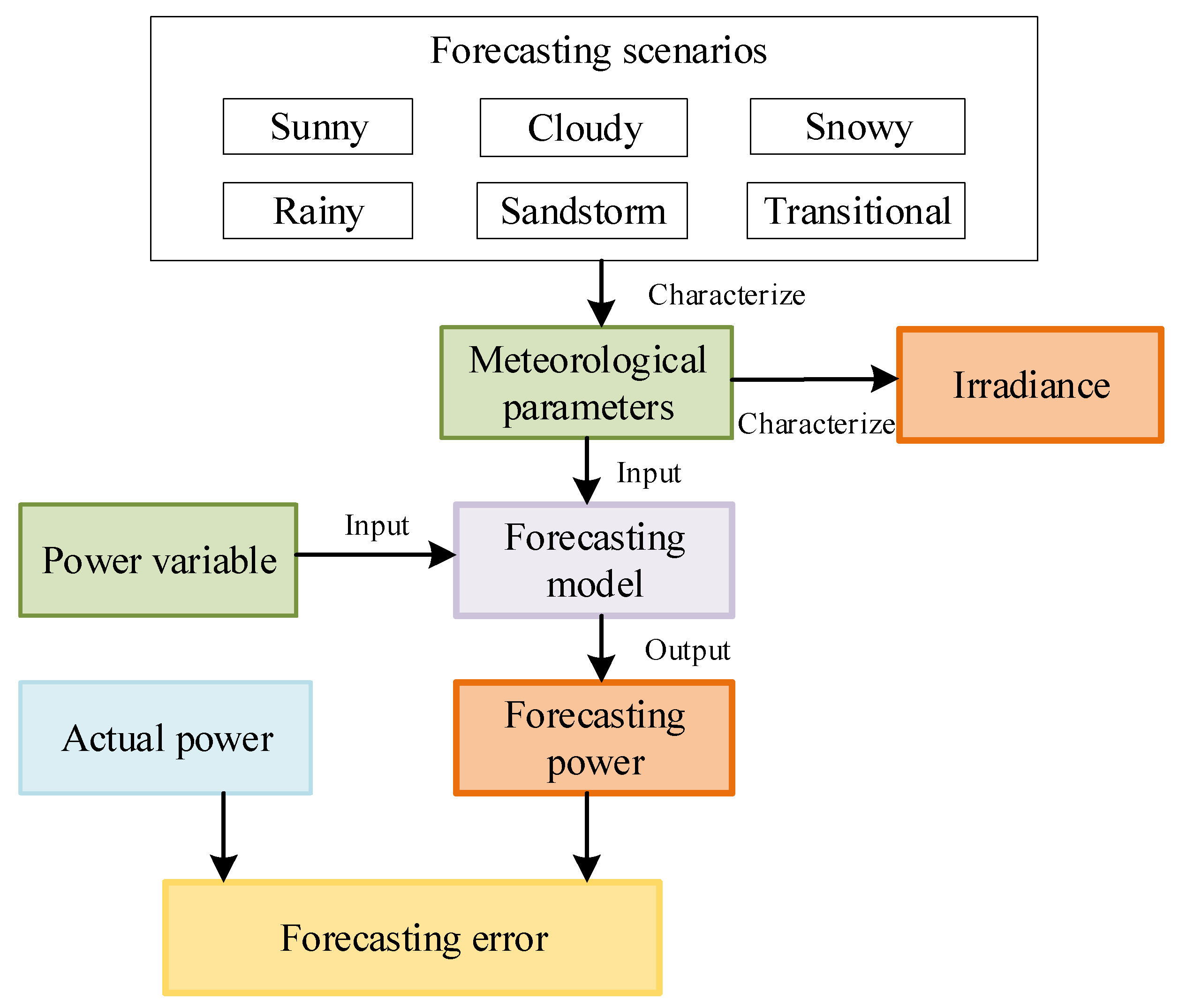
The conditions contributing to forecasting errors in PV power generation are analyzed in Figure 2. Forecasting errors are directly determined by the discrepancy between measured and forecasted power, where forecasted power depends on the forecasting model and its input variables—with irradiance being one of the most critical inputs. As a meteorological variable highly correlated with PV power output, irradiance partially reflects the characteristics of the forecasting scenario. Simultaneously, the performance of power forecasting models often varies across different forecasting scenarios. Therefore, forecasting errors are ultimately determined by both the forecasting scenario and the forecasting model.

3.1.2. Dynamic Coupling Characteristics Analysis

The mapping relationship between irradiance and PV power output is not static. As a PV system operates over time, module performance gradually changes due to various factors. For example, during long-term operation, PV modules experience phenomena such as light-induced degradation [19], potential-induced degradation [20], and aging of encapsulation materials; these factors all lead to a gradual decline in module output efficiency. Furthermore, factors such as dust accumulation on the module surface, changes in ambient temperature, and increases in module temperature can also alter the module’s PV conversion efficiency, thereby affecting the functional relationship between irradiance and output power.

In addition to the aforementioned long-term factors, in the short term, the mapping relationship between forecasted irradiance and forecasting power varies under different weather conditions, and the coupling relationship among forecasted irradiance, forecasting power, and forecasting error consequently changes as well.

Due to the combined effects of the aforementioned factors, the operational characteristics of PV systems exhibit significant time-varying behavior, and the relationships between variables change over time. This variability causes forecasting models established based on historical data to degrade in performance or even fail over time. Therefore, when conducting probabilistic power forecasting for PV systems, it is necessary not only to consider the changing mapping relationship between predicted irradiance and forecasting power but also to account for the dynamic characteristics of forecasting errors that evolve over time. In other words, the correlation structure among predicted irradiance, forecasting power, and forecasting error is not static but varies dynamically with operational conditions and environmental factors. Based on this characteristic, this paper employs dynamic multivariate Copula functions in the modeling process to characterize the time-varying correlations among these three variables, thereby enabling a more accurate description of their joint probability distribution characteristics and enhancing the reliability of probabilistic PV power forecasting.

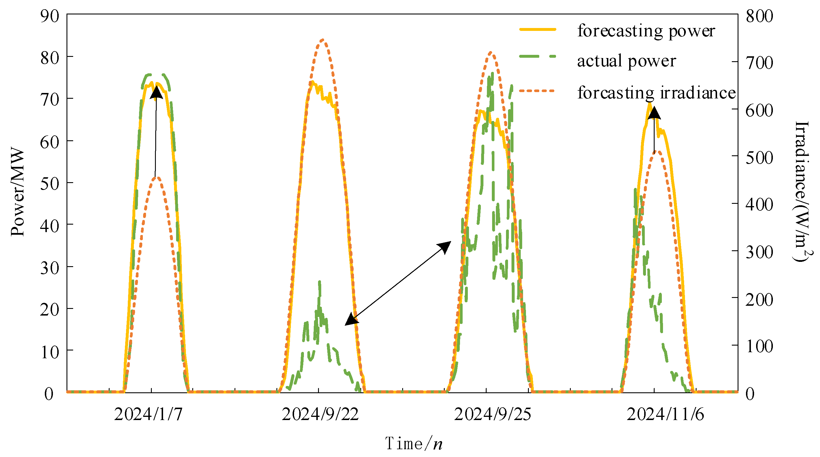
As shown in Figure 3, the predicted irradiance values for 22 September and 25 September are similar, and the corresponding power forecasting is also close. However, the measured values differ significantly, resulting in substantial variations in the error sequence. Conversely, on 7 January and 6 November, the predicted irradiance values differ, yet the power forecasting is roughly the same, while the measured power values also vary. This demonstrates that the coupling relationship among predicted irradiance, forecasting power, and forecasting error evolves over time.

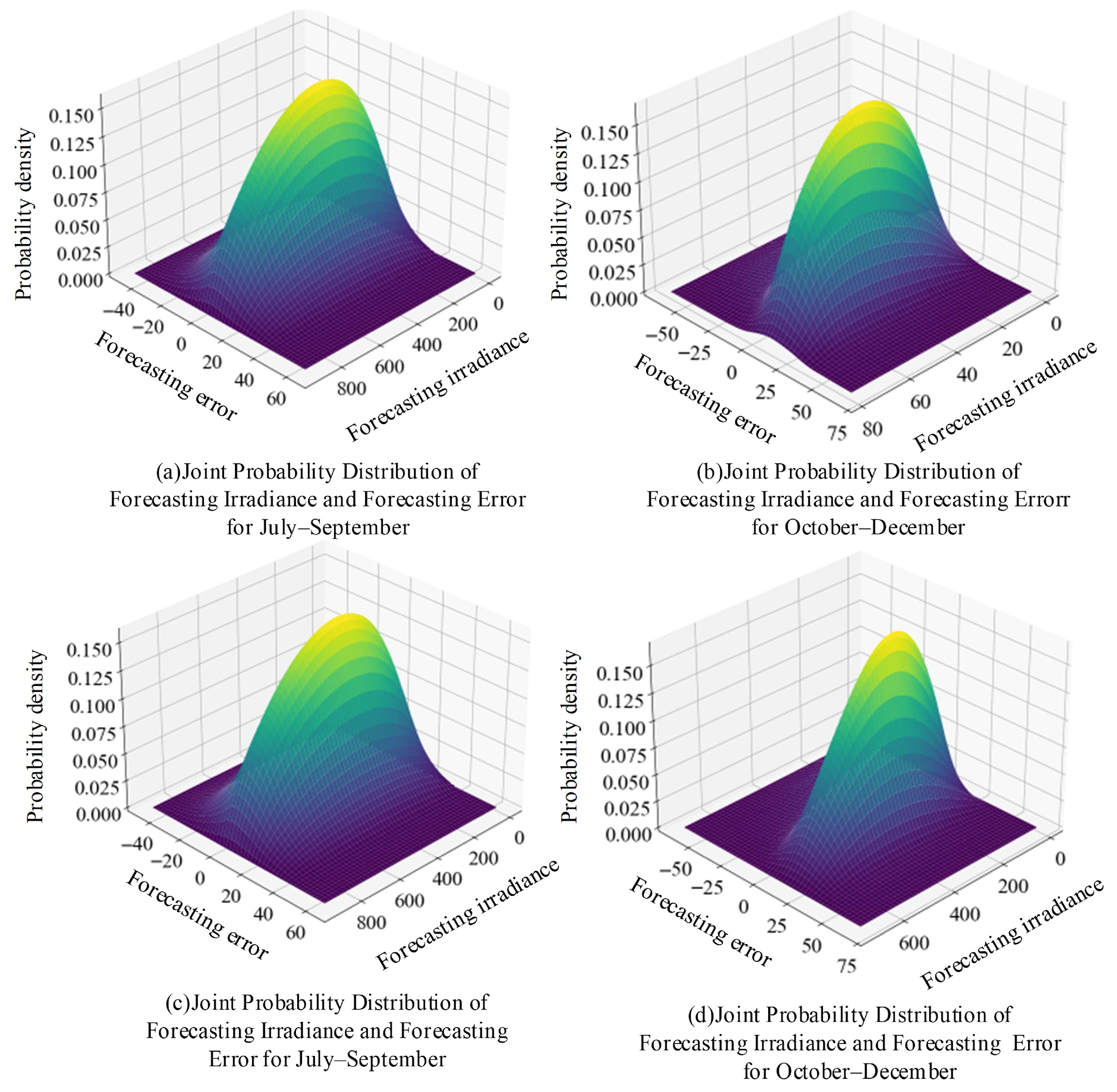
Figure 4 illustrates the joint probability density curves of forecasting power and predicted irradiance versus forecasting error across different seasons over time. It reveals that the shape of these joint probability density curves changes with time, indicating that the coupling characteristics among variables exhibit dynamic variability.

3.2. Principles of the Copula Function

When different random variables are not independent of each other, modeling their joint distribution becomes highly challenging. Copula functions are multidimensional joint distribution functions with a uniform distribution over the domain (0,1). Their core concept involves coupling the marginal distributions of multiple random variables using copula functions, thereby enabling the modeling of multivariate joint distributions [21].

According to Sklar’s theorem, for any joint distribution function F, there exists a copula function C such that:

$$F(x_1,x_2,\dots ,x_m)=C(F_1(x_1),F_2(x_2),\dots ,F_n(x_n))$$

(1)

where $u_i=F_i(x_i)\in [0,1]$, $F_i(x_i)$ denotes the marginal distribution of each variable, and $F(x_1,x_2,\dots ,x_m)$ represents the joint probability distribution. If all F_i are continuous, then C is unique.

Copula functions describe the dependence relationships between variables without relying on the specific forms of their marginal distributions.

Copula functions come in various forms, such as Gaussian Copula, t-Copula, and Clayton Copula. Different types of Copulas vary in structure and characteristics, thus exhibiting distinct advantages and disadvantages when modeling dependence relationships between variables. For instance, the Gaussian Copula model features a simple structure, high computational efficiency, and stable parameter estimation [19], but it cannot capture tail dependencies. Conversely, the t-Copula can model two-tailed dependencies, yet it involves more complex parameter estimation and carries a certain risk of overfitting. Precisely because different Copula functions vary in their description of dependency structures, it is necessary in practical applications to comprehensively consider and combine multiple Copulas to more accurately reflect the associative characteristics between variables.

Given that forecasting errors are predominantly clustered around zero, their distribution function exhibits symmetry. Therefore, two copula functions with symmetric properties—the Gaussian Copula and the t-Copula—were selected.

The Gaussian Copula is expressed as:

$$C_{\mathrm{\Sigma }}^{\mathrm{Gauss}}(u_1,\dots ,u_n)={\mathrm{\Phi }}_{\mathrm{\Sigma }}\left({\mathrm{\Phi }}^{-1}(u_1),\dots ,{\mathrm{\Phi }}^{-1}(u_n)\right)$$

(2)

where ${\mathrm{\Phi }}^{-1}(•)$ is the inverse function of the standard normal distribution, and ${\mathrm{\Phi }}_{\mathrm{\Sigma }}\left(•\right)$ is the joint distribution function of multivariate normal distributions with correlation matrix Σ.

The expression for the t-Copula is:

$$C_{\mathrm{\Sigma },\nu }^{\mathrm{t}}(u_1,\dots ,u_n)=t_{\mathrm{\Sigma },\nu }\left(t_{\nu }^{-1}(u_1),\dots ,t_{\nu }^{-1}(u_n)\right)$$

(3)

where $t_{\nu }^{-1}(•)$ is the inverse function of the t-distribution with $\upsilon$ degrees of freedom, and $t_{\mathrm{\Sigma },\nu }\left(•\right)$ is the multivariate t-distribution with correlation matrix $\sum$ and $\upsilon$ degrees of freedom. The t-distribution exhibits “thicker” tails compared to the normal distribution, thereby reflecting stronger correlations in tail events—that is, it better captures the interdependencies among variables under extreme scenarios.

3.3. Construction of Dynamic High-Dimensional Copula Functions

Since probabilistic forecasting is ultimately achieved through the probability interval of forecasting errors, it is necessary to analyze the conditional distribution of these errors—that is, how forecasting errors are distributed under different conditions. The finer the conditions, the more accurate the forecasting errors become. However, although elliptical copula functions inherently support constructing joint probability distributions for multiple random variables, increasing the number of fitted variables significantly elevates the parameter dimension, computational complexity, and data requirements of the copula model. This leads to risks such as overfitting, unstable estimates, and distorted dependency structures. Therefore, when applying copula functions in practice, it is essential to control the number of fitted random variables by extracting key variables. As described in Section 3.1.1, the forecasting power and forecasted irradiance are extracted as the conditions generating forecasting errors, thereby fitting the joint probability distribution function of forecasting power, forecasted irradiance, and forecasting errors.

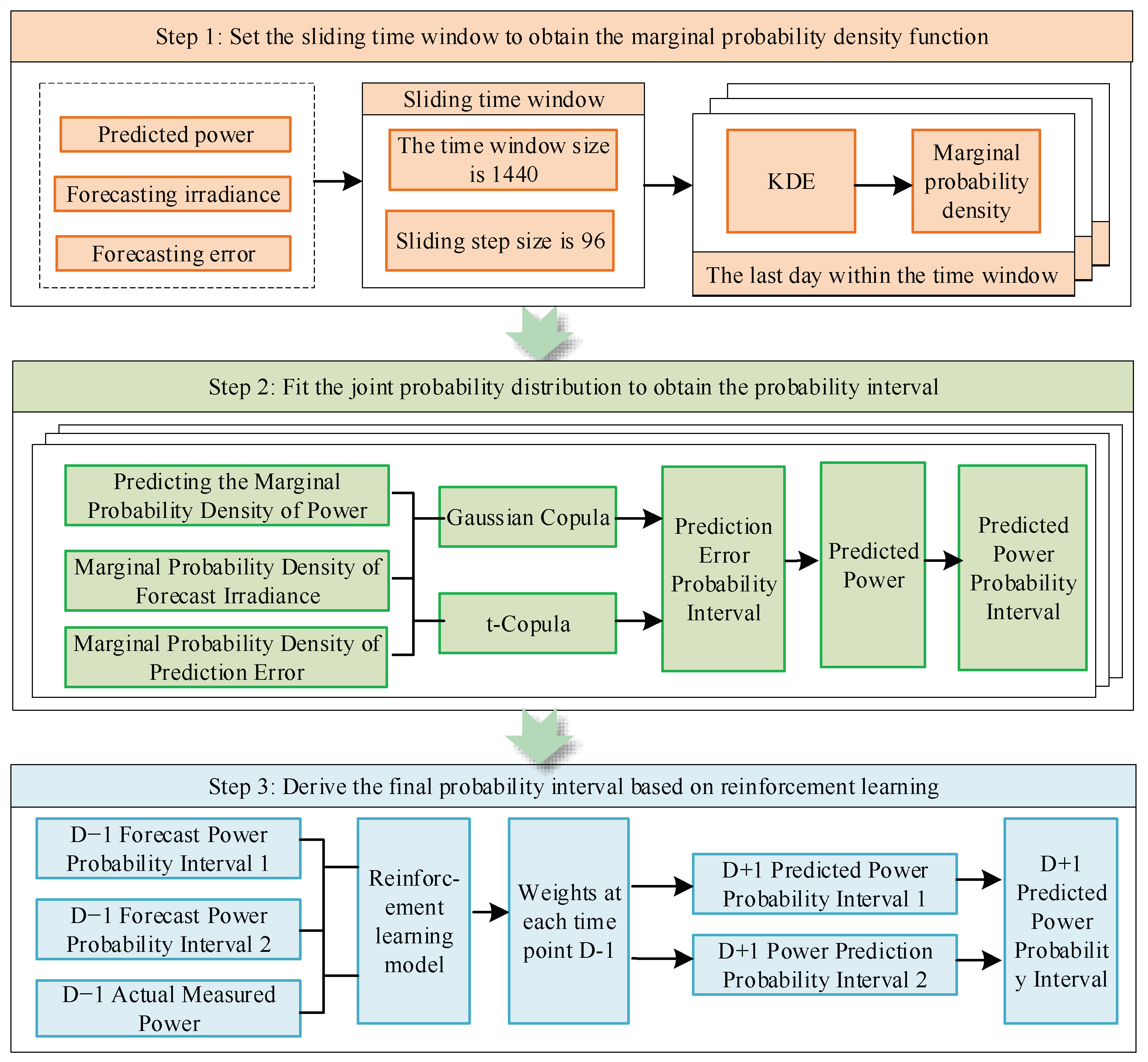
This paper employs a sliding time window mechanism to capture the dynamic characteristics of variables. Given that insufficient data within a time window can lead to unstable estimates of Copula function parameters, appropriately expanding the time window helps the model learn more stable statistical features; however, if the time window is too long, it may introduce excessive non-stationary variations, thereby weakening the model’s ability to capture local correlation structures. Therefore, a trade-off must be struck between sample stability and the capture of dynamic characteristics. Based on the above considerations, and given that the data has a 15-min time resolution, this paper empirically selects a time window length of 1440, corresponding to 15 days of data.

Furthermore, considering that day-ahead forecasts require daily rolling updates, this study sets the time window sliding step to 96 (i.e., one day’s worth of data). Specifically, within each time window, the three-dimensional Copula function is fitted using data from the preceding 14 days, and the forecasting error for the 15th day is probabilistically modeled based on the resulting joint probability distribution, thereby obtaining the corresponding PV power forecast interval.

3.3.1. Gaussian Copula

The construction process of the Gaussian Copula function comprises the following three steps:

(1) Use kernel density estimation to fit the marginal probability density functions of forecasting error, forecasting power, and forecast irradiance within the time window.

Kernel density estimation is a nonparametric method for estimating the probability density function of data [22]. It relies on kernel functions with a given bandwidth parameter to estimate the probability density at each data point by performing a weighted average of kernel functions near that point. The Gaussian kernel function is typically chosen, expressed as follows:

$$K(x)={\displaystyle \frac{1}{\sqrt{2\mathrm{\pi }}}}\exp \left(-{\displaystyle \frac{x^2}{2}}\right)$$

(4)

where $x$ is the input value, and $K(x)$ is the value of the Gaussian kernel function.

Based on the kernel function, the probability density is calculated as follows:

$$f(x)={\displaystyle \frac{1}{nh}}{\displaystyle \sum _{i=1}^{n}K}\left({\displaystyle \frac{x-x_i}{h}}\right)$$

(5)

where n is the sample size, and h is the bandwidth.

Let the three variables of forecasted irradiance, forecasting power, and forecasting error be denoted as $X_1$, $X_2$, and $X_3$, respectively. Then the resulting marginal distributions and densities are $F_i\left(X_i\right)$ and $f_i\left(X_i\right)$, respectively, where $i=1,2,3$.

(2) Map the original variables to standard normal variables

Let $U_i=F_i\left(X_i\right)$, then $U_i\sim \mathrm{Uniform}\left(0,1\right)$. Then transform the uniform variables into standard normal variables:

$$Z_i={\mathrm{\Phi }}^{-1}\left(U_i\right)={\mathrm{\Phi }}^{-1}\left(F_{-1}\left(X_i\right)\right)\sim N\left(0,1\right)$$

(6)

where ${\mathrm{\Phi }}^{-1}$ is the inverse cumulative distribution function of the standard normal distribution.

Then obtain the random variable $Z={(Z_1,Z_2,Z_3)}^{\top }\sim N(0,\mathrm{\Sigma })$, where $\mathrm{\Sigma }$ is the correlation matrix between the variables.

(3) Constructing Gaussian Copulas

Let $z={\left(z_1,z_2,z_3\right)}^{\mathrm{T}}$ denote the vector formed by the combinations of values taken by the random variables Z₁, Z₂, and Z₃. The density expression for the multivariate normal distribution is:

$${\phi }_{\mathrm{\Sigma }}(z)={(2\mathrm{\pi })}^{-3/2}|\mathrm{\Sigma }{|}^{-1/2}\exp \left(-{\displaystyle \frac{1}{2}}{z}^{\top }{\mathrm{\Sigma }}^{-1}z\right)$$

(7)

Since the first-order standard normal density is $\phi (z)={(2\mathrm{\pi })}^{-{\displaystyle \frac{1}{2}}}{e}^{-{\displaystyle \frac{z^2}{2}}}$, the copula density is:

$$c_{\mathrm{\Sigma }}(u_1,u_2,u_3)={\displaystyle \frac{{\phi }_{\mathrm{\Sigma }}(z)}{\phi (z_1)\phi (z_2)\phi (z_3)}}=|\mathrm{\Sigma }{|}^{-1/2}\exp \left(-{\displaystyle \frac{1}{2}}{z}^{\top }({\mathrm{\Sigma }}^{-1}-I)z\right)$$

(8)

The three-dimensional joint density is given by the combination of the copula function and the marginal functions:

$$f_X(x_1,x_2,x_3)=c_{\mathrm{\Sigma }}\left(F_1(x_1),F_2(x_2),F_3(x_3)\right)•f_1(x_1)f_2(x_2)f_3(x_3)$$

(9)

Substituting expression $c_{\mathrm{\Sigma }}$ into $z_i{=\mathrm{\Phi }}^{-1}\left(F_{-1}\left(x_i\right)\right)$ yields the joint probability density of the original variables:

$$f_X(x_1,x_2,x_3)=|\mathrm{\Sigma }{|}^{-1/2}\exp \left(-{\displaystyle \frac{1}{2}}{z}^{\top }({\mathrm{\Sigma }}^{-1}-I)z\right){\displaystyle \prod _{i=1}^3{f}_i}(x_i)$$

(10)

3.3.2. t-Copula

The construction process of the t-Copula function involves the following three steps:

(1) Similar to the Gaussian Copula, map the original variables X_i to the marginal distribution probability intervals:

$$u_i=F_i(x_i),\hspace{1em}i=1,2,3$$

(11)

(2) Transform the marginal probability distribution into the t-distribution space:

$$t_i=t_{\nu }^{-1}(u_i)$$

(12)

where $t_{\nu }^{-1}(•)$ is the inverse cumulative distribution function (CDF) of the one-dimensional Student-t distribution with ν degrees of freedom.

(3) Constructing the t-Copula

The cumulative distribution function (CDF) expression for the t-Copula is:

$$C_{\mathrm{\Sigma },\nu }(u_1,u_2,u_3)=t_{\mathrm{\Sigma },\nu }\left(t_{\nu }^{-1}(u_1),t_{\nu }^{-1}(u_2),t_{\nu }^{-1}(u_3)\right)$$

(13)

In the equation, $\mathrm{\Sigma }$ denotes the copula’s correlation matrix, and $\nu$ represents the degrees of freedom parameter.

The probability density function of the t-Copula is:

$$\begin{array}{cc}{c}_{\mathrm{\Sigma },\nu }(u_1,u_2,u_3)\hfill & ={\displaystyle \frac{t_{\mathrm{\Sigma },\nu }(t)}{{\displaystyle \prod _{i=1}^3{t}_{\nu }}(t_i)}}\hfill \\ & =|\mathrm{\Sigma }{|}^{-1/2}{\displaystyle \frac{\mathrm{\Gamma }\left(\frac{\nu +3}{2}\right)}{\mathrm{\Gamma }\left(\frac{\nu }{2}\right)}}•\left({\displaystyle \prod _{i=1}^3\frac{\mathrm{\Gamma }\left(\frac{\nu }{2}\right)}{\mathrm{\Gamma }\left(\frac{\nu +1}{2}\right)}}\right){\left(1+{\displaystyle \frac{1}{\nu }}{t}^{\top }{\mathrm{\Sigma }}^{-1}t\right)}^{-{\displaystyle \frac{\nu +3}{2}}}{\displaystyle \prod _{i=1}^3\left(1+\frac{t_i^2}{\nu }\right)}\hfill \end{array}$$

(14)

where $\mathrm{\Gamma }\left(•\right)$ is the function describing the characteristics of the degrees of freedom in the t-distribution, ${\left(1+{\displaystyle \frac{1}{\nu }}{t}^{\top }{\mathrm{\Sigma }}^{-1}t\right)}^{-{\displaystyle \frac{\nu +3}{2}}}$ is the core exponential term of the multivariate t-distribution density, reflecting the decaying properties of fat-tail dependencies, and ${\displaystyle \prod _{i=1}^3\left(1+\frac{t_i^2}{\nu }\right)}$ is the product term of the univariate t-distribution density, used to isolate the influence of marginal distributions.

Based on this, the joint probability density function of the original variables is:

$$f_{X_1,X_2,X_3}(x_1,x_2,x_3)=c_{\mathrm{\Sigma },\nu }\left(F_1(x_1),F_2(x_2),F_3(x_3)\right){\displaystyle \prod _{i=1}^3{f}_i}(x_i)$$

(15)

3.4. Copula Parameter Estimation and Update Process

Within each sliding window, the Copula parameters are estimated through the following steps:

(1) Estimation of marginal distributions:

First, the marginal distributions of each variable are estimated. Since the distributions of PV power and irradiance typically exhibit nonparametric characteristics, this paper employs kernel density estimation (KDE) to obtain the probability density functions for the forecast irradiance, predicted power, and forecasting error, denoted as $f_X\left(x\right)$, $f_Y\left(y\right)$, and $f_Z\left(z\right)$, respectively. These are then transformed into standard normal variables via the cumulative distribution function, resulting in $u_t=F_X\left(x_t\right)$, $v_t=F_Y\left(y_t\right)$, and $w_t=F_Z\left(z_t\right)$, respectively.

(2) Estimation of Copula-related structures:

After obtaining the uniform variables, the three-dimensional joint distribution is constructed using the Copula function as follows:

$$C\left(u_t,v_t,w_t;\theta \right)$$

(16)

In the equation, $C\left(•\right)$ denotes the Copula function, and $\theta$ represents the Copula parameters.

The parameters are estimated using maximum likelihood estimation within each time window:

$${\theta }_k=\arg {\max }_{\theta }{\displaystyle \sum _{t=1}^W\ln }c(u_t,v_t,w_t;\theta )$$

(17)

In the equation, $c\left(•\right)$ represents the Copula density function, and W represents the number of samples in the window.

(3) Sliding Window Update Mechanism

As the time window progresses, the samples used to fit the Copula function within the window also change; the relevant parameters of the Copula function are re-estimated using the new samples within each time window.

3.5. Solving the Probability Interval of Forecasting Error

Based on the constructed Gaussian Copula and t-Copula, the probability distribution function of forecasting errors under each conditional distribution is derived using the conditional distribution and the forecasted irradiance and forecasting power at each future time step. This enables the determination of upper and lower bounds for forecasting errors at different confidence levels. The conditional distribution functions for forecasting errors corresponding to the Gaussian Copula and t-Copula are respectively:

$$F_{X_3|X_1,X_2}^{\mathrm{Gauss}}(x_3|x_1,x_2)=P(X_3\le x_3|X_1=x_1,X_2=x_2)=\mathrm{\Phi }\left({\displaystyle \frac{{\mathrm{\Phi }}^{-1}(F_3(x_3))-{\mu }_{3|12}}{{\sigma }_{3|12}}}\right)$$

(18)

$$F_{X_3|X_1,X_2}^t(x_3|x_1,x_2)=P(X_3\le x_3|X_1=x_1,X_2=x_2)=T_{\nu +2}\left({\displaystyle \frac{t_{\nu }^{-1}(F_3(x_3))-{\mu }_{3|12}^{(t)}}{{\sigma }_{3|12}^{(t)}}}\right)$$

(19)

where X₁, X₂, and X₃ represent the forecasting power, forecasted irradiance, and forecasting error, respectively. $x_1$, $x_2$ and $x_3$ denote the specific values of the three random variables. ${\mu }_{3|12}$ and ${\sigma }_{3|12}$ are the conditional mean and conditional standard deviation of X₃ given X₁ and X₂, respectively. $T_{\nu +2}\left(•\right)$ is the cumulative distribution function of the t-distribution with $\nu +2$ degrees of freedom.

3.6. Combination Strategy Based on Deep Reinforcement Learning

Reinforcement learning is a method enabling agents to learn optimal behavioral strategies through interaction with their environment. Agents continuously experiment with actions, observe outcomes, and adjust their strategies based on reward signals. Ultimately, they learn to take optimal actions in various scenarios to maximize long-term benefits. Reinforcement learning can be categorized into two main types: value-based reinforcement learning and policy-based reinforcement learning. Proximal Policy Optimization (PPO) is a policy-based reinforcement learning method that maximizes expected return by directly optimizing the policy function [23].

This paper trains a reinforcement learning model for dynamically combining probability intervals. It uses the upper and lower bounds of the two probability intervals from the previous day as input variables (states), the fused weights across 96 time points of that day as output variables (actions), and the negative value of the Winkler score from the combined probability interval as the reward.

3.6.1. Strategy Update Objectives

Set the policy to ${\pi }_{\theta }(a|s)$; the fundamental objective of policy gradient methods is to maximize the following surrogate objective function:

$$L(\theta )={\mathbb{E}}_t\left[r_t(\theta ){\widehat{A}}_t\right]$$

(20)

where $r_t(\theta )={\displaystyle \frac{{\mathrm{\pi }}_{\theta }(a_t|s_t)}{{\mathrm{\pi }}_{{\theta }_{\mathrm{old}}}(a_t|s_t)}}$ denotes the probability ratio of the new and old policies for a unified action, while ${\widehat{A}}_t$ is the advantage function used to measure action quality.

3.6.2. Cutting Objective Function

The core objective function of PPO is defined as:

$$L^{CLIP}(\theta )={\mathbb{E}}_t\left[\min \left(r_t(\theta ){\widehat{A}}_t,\mathrm{clip}(r_t(\theta ),1-ϵ,1+ϵ){\widehat{A}}_t\right)\right]$$

(21)

where $\mathrm{clip}(r_t(\theta ),1-ϵ,1+ϵ){\widehat{A}}_t$ is a shear operation that constrains $r_t(\theta )$ within the interval $\left[1-ϵ,1+ϵ\right]$, ${\mathbb{E}}_t\left[•\right]$ denotes the expectation over time step t.

3.6.3. Advantage Function Estimation

To enhance the sample efficiency and stability of policy gradient methods, PPO predominantly employs generalized advantage estimation, where the advantage function is defined as:

$${\widehat{A}}_t={\displaystyle \sum _{l=0}^{\infty }{(\gamma \lambda )}^l}{\delta }_{t+l}$$

(22)

where ${\widehat{A}}_t$ is the advantage estimate at time step t, measuring the “advantage” of selecting action $s_t$ over the average action $a_t$ in state $s_t$. $\gamma$ is the discount factor, $\lambda$ is the decay coefficient for the generalized advantage estimate, and ${\delta }_{t+l}$ is the temporal difference residual at time step t + l, quantifying the discrepancy between the current estimate and the next-step estimate.

3.6.4. Training Process

For the probability interval of the forecasting power, this paper employs the following three metrics to evaluate its predictive performance [24]:

(1) Reliability Index R_a: Represents the difference between the predicted interval coverage and the preset confidence level. The closer it approaches 0, the higher the reliability of the probability interval. The calculation formula is:

$$R_a=I_{\mathrm{PICP}}-a={\displaystyle \frac{1}{N}}{\displaystyle \sum _{i=1}^N{k}_{na}}-a$$

(23)

In the formula, $k_{ia}$ is a Boolean value. When the actual power value of sample $n$ falls within the predicted interval under a given confidence level $a$, then $k_{na}=1$; otherwise, $k_{na}=0$.

(2) Prediction Interval Average Width $S$: Represents the average width of the prediction interval. A narrower interval indicates higher sharpness, signifying greater prediction accuracy. The calculation formula is:

$$S={\displaystyle \frac{1}{N}}{\displaystyle \sum _{i=1}^N(U_i-L_i)}$$

(24)

In the formula, $U_i$ and $L_i$ represent the upper and lower bounds of the prediction interval for sample size n, respectively, and $N$ denotes the total number of samples.

(3) Winkler Score $S_{\mathrm{W}}$: Evaluates overall performance by weighting the reliability and sharpness of intervals, with lower scores indicating better performance. The calculation formula is:

$$S_{\mathrm{W}}=(U_i-L_i)+{\displaystyle \frac{2}{\tau }}(L_i-P_i)x(L_i-P_i)+{\displaystyle \frac{2}{\tau }}(P_i-U_i)x(P_i-U_i)$$

(25)

$$v(x)=\left\{\begin{array}{ll}1,\hfill & x\ge 0\hfill \\ 0,\hfill & x<0\hfill \end{array}\right.$$

(26)

where $(U_i-L_i)$ represents an assessment of the sharpness of the prediction interval; the wider the interval, the larger this term becomes. The subsequent two terms evaluate the reliability of the prediction interval. When the actual value falls outside the prediction interval, these two terms are positive, indicating a penalty for forecasting errors; when the actual value falls within the prediction interval, these two terms are zero.

4. Case Study

4.1. Data Description

This study conducts experiments using actual power output, forecasting power output, actual meteorological data, and forecasted meteorological data provided by a PV power station in Shanxi Province to validate the effectiveness of the proposed method. The data span from 1 September 2024 to 1 September 2025, with a 15-min resolution. The test set covers the period from 1 August 2025 to 1 September 2025. Given the significant variations in PV power generation patterns across different regions and climatic conditions, this paper also employs data from a PV power plant in the Inner Mongolia Autonomous Region to conduct cross-climatic validation, thereby enhancing the method’s generalizability. The data covers the period from 1 January 2024 to 31 December 2024, with a resolution of 15 min; the test set spans from 1 December 2024 to 31 December 2024.

4.2. Comparative Experiment

To fully validate the effectiveness of the proposed method in this paper, comparative experiments were conducted using the following approaches:

Method 1: Probabilistic forecasting was performed by fitting the joint probability distribution of forecasted irradiance, forecasting power, and forecasting error using only the dynamic t-Copula function;

Method 2: Probabilistic forecasting was performed by fitting the joint probability distribution of forecasted irradiance, forecasting power, and forecasting error using only the dynamic Gaussian Copula function;

Method 3: Fit the joint probability distribution of forecasted irradiance, forecasted power, and forecasted error using static t-Copula and static Gaussian Copula functions respectively, then combine the probabilistic forecasting results;

Method 4: Fit the joint probability distribution of forecasted power and forecasted error using dynamic t-Copula and dynamic Gaussian Copula functions respectively, then combine the probabilistic forecasting results.

Method 5: Use the Gaussian Copula and t-Copula functions separately to fit the joint probability distributions of the forecast temperature, forecasting power, and forecasting error, and then combine the probability forecasting results.

4.3. Results Display

4.3.1. Joint Probability Density and Joint Probability Distribution

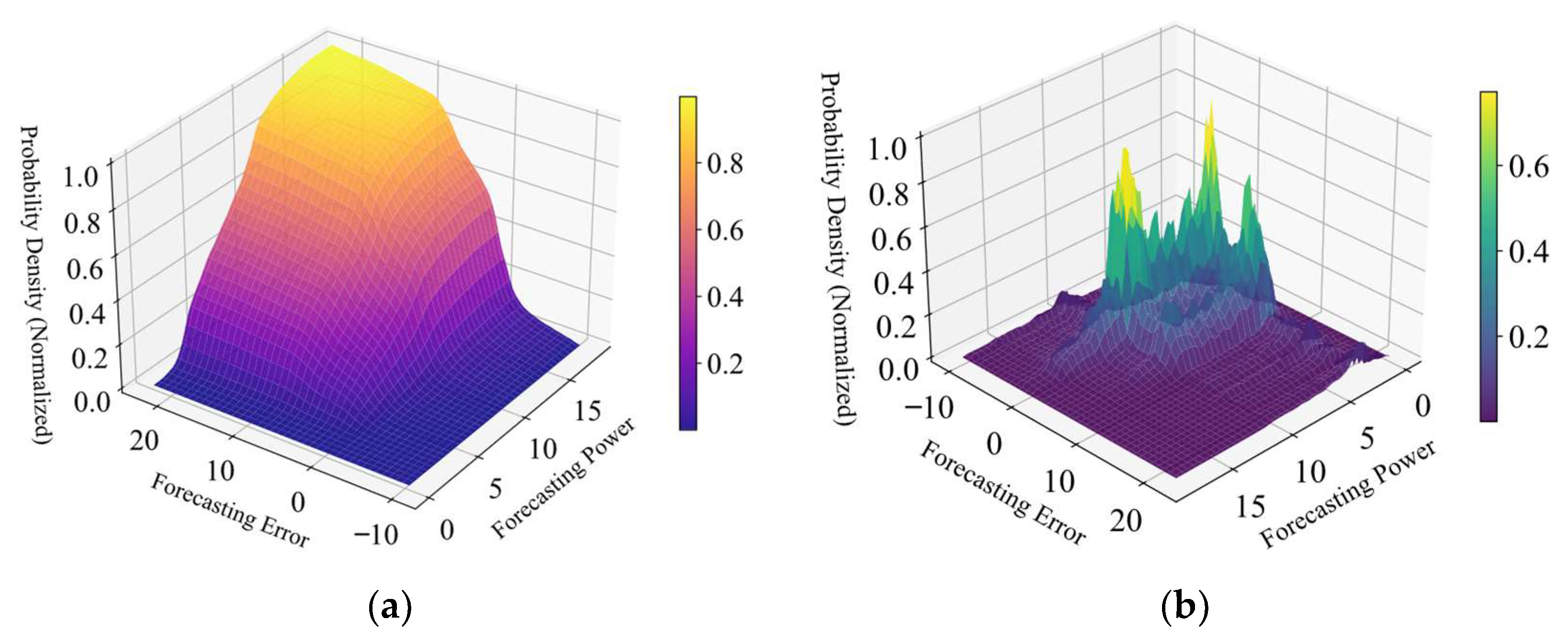
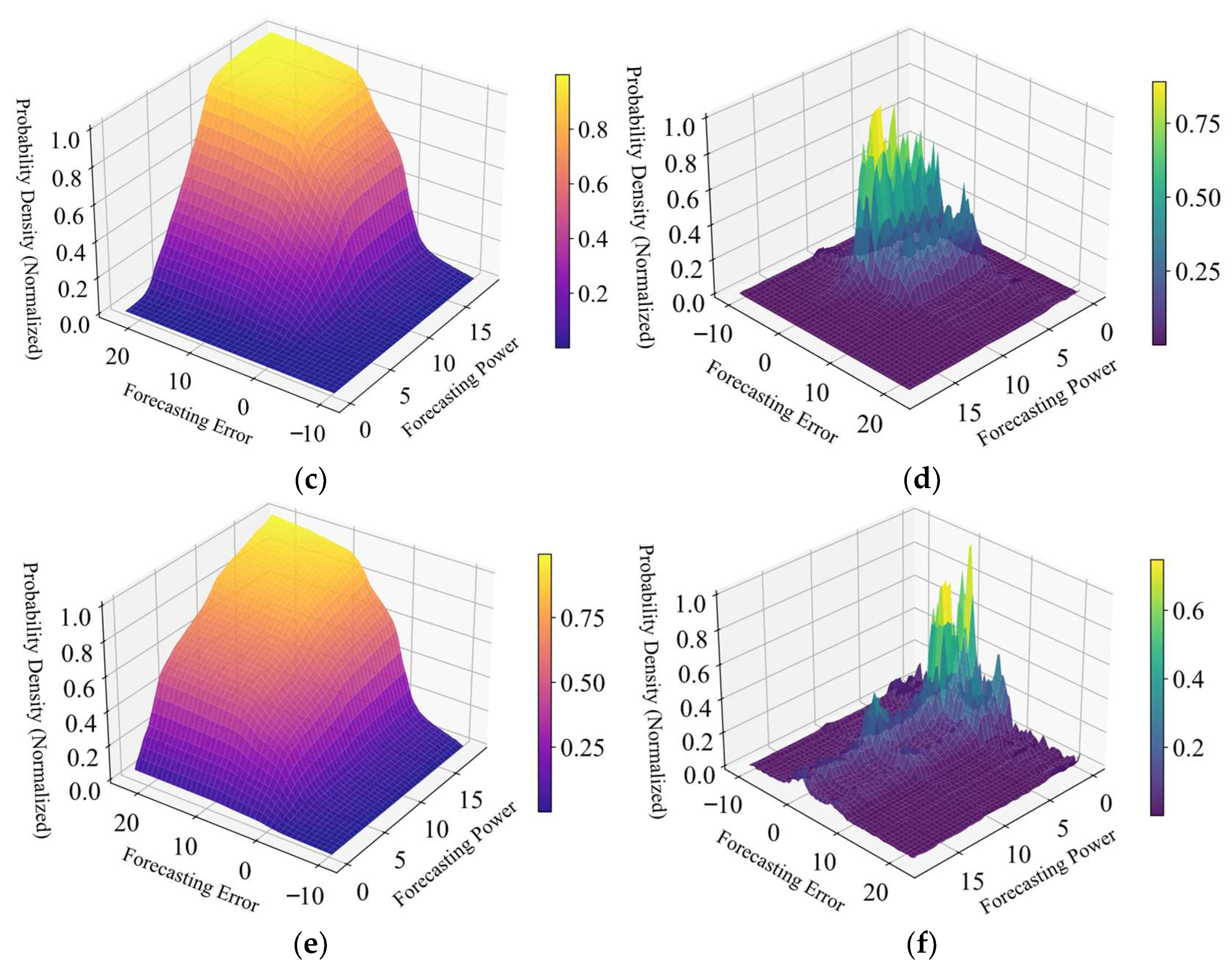
Figure 5a,b show the Gaussian Copula joint probability distribution function and t-Copula joint probability distribution function for forecasting power and forecasting error when the forecast irradiance is fixed at 300 W/m² within the 12th time window. Figure 5d,e present the corresponding probability density functions, while Figure 5c,f display the joint probability distribution functions and probability density functions of the forecasted power and forecasted error obtained by fitting within the 12th time window. The cumulative probabilities of all three cumulative probability distributions reach 1 when the forecasting power and forecasting error attain their maximum values, consistent with the fundamental definition of cumulative probability distributions. Meanwhile, the peaks of the probability density functions occur around a forecasting error of 0, aligning with the general principle that power forecasting results rarely deviate significantly from measured power, and small errors are highly probable events. As shown in Figure 5, different Copula functions yield distinct probability distributions and probability densities for the same data set. Similarly, varying the number of fitted variables under the same Copula function produces differing probability distributions and densities.

4.3.2. Probability Forecasting Results

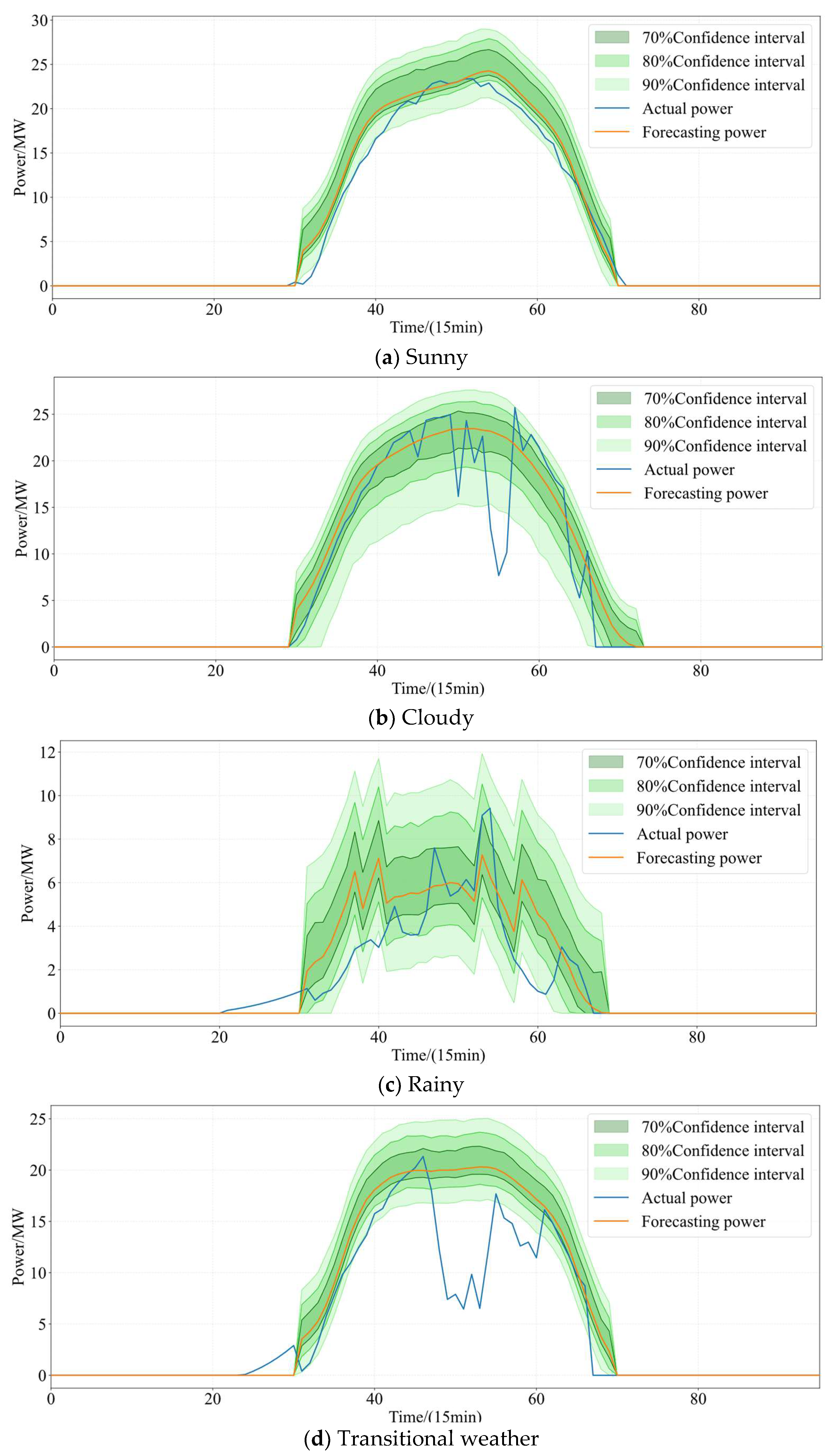
Figure 6 presents probability forecasts obtained using the proposed method under several typical weather conditions. To highlight forecast details, only four representative days are shown.

Table 1. Evaluation Indicator Calculation Results.

Method	Confidence Level	Reliability Index	Prediction Interval Average Width	Winkler Score
Proposed Method	70%	−0.038	1.195	2.884
Method1		−0.570	1.195	2.984
Method 2		−0.047	1.195	2.983
Method 3		−0.010	1.454	3.114
Method 4		−0.040	1.290	3.076
Method 5		−0.128	5.418	7.319
Proposed Method	80%	−0.066	2.042	3.123
Method1		−0.656	2.042	3.322
Method 2		−0.085	2.043	3.325
Method 3		−0.014	2.684	3.790
Method 4		−0.074	2.084	3.401
Method 5		−0.126	7.0531	8.410
Proposed Method	90%	−0.073	3.451	4.063
Method1		−0.738	3.447	4.160
Method 2		−0.095	3.455	4.167
Method 3		−0.030	4.451	5.093
Method 4		−0.086	3.433	4.184
Method 5		−0.132	9.735	10.515

presents the results of various evaluation metrics obtained by comparing the method proposed in this paper with four control methods on a test set using actual data from a power plant in Shanxi Province, under three confidence levels of 90%, 80%, and 70%.

Table 2. The calculation results of the evaluation indicators obtained from the data of Inner Mongolia.

Method	Confidence Level	Reliability Index	Prediction Interval Average Width	Winkler Score
Proposed Method	70%	−0.10373	27.38766	35.37767
Method1		−0.0383	27.39	36.72682
Method 2		−0.05434	42.6217	57.34203
Method 3		−0.37675	16.78194	39.28067
Method 4		−0.06048	43.2052	57.45294
Method 5		−0.05434	42.61591	57.34531
Proposed Method	80%	−0.11611	22.06134	40.79764
Method1		−0.03775	35.74517	42.40075
Method 2		−0.04693	55.25488	65.60364
Method 3		−0.38266	35.75418	41.29301
Method 4		−0.05051	55.3217	65.4503
Method 5		−0.04539	55.26146	65.61346
Proposed Method	90%	−0.03388	31.85307	45.97291
Method1		−0.02983	47.92663	52.00003
Method 2		−0.12188	47.92558	50.1232
Method 3		−0.34388	71.47216	77.99926
Method 4		−0.03149	71.16241	77.59206
Method 5		−0.03439	71.46744	78.00439

presents the comparison results of the evaluation metrics for the aforementioned methods using actual data from a power plant in the Inner Mongolia Autonomous Region, under the same test conditions and confidence level settings.

Since the prediction method proposed in this paper involves multiple steps, it is necessary to specify the model runtime. Fitting the Gaussian Copula model on the full dataset used in this study took 179.74 s, fitting the t-Copula model took 320.27 s, and generating probability intervals for the three confidence levels using reinforcement learning took 132.86 s, for a total runtime of 632.87 s. All of the above experiments were conducted on a single personal computer with the following specifications: a Lenovo Xiaoxin 15 laptop equipped with an Intel Core i5 processor and 16 GB of RAM. In practical applications, however, daily forecasting requires only the fitting and combination of models within a single time window; furthermore, since the program will run on high-performance servers at the power plant, the computation time will be significantly reduced.

4.4. Results Analysis

Figure 6 results indicate that under clear weather conditions, prediction is relatively straightforward with minimal deviation, and most measured values fall within the 70% confidence interval. Conversely, during periods of significant weather variability, while individual measured power values occasionally fall outside the 90% confidence interval, the remaining instances are fully covered by it. Comparing Figure 6a,b reveals that the measured and forecasting power levels are broadly similar, though their probability intervals differ. Meanwhile, Figure 6c demonstrates that even under cloudy and rainy conditions, the probability interval still encompasses the actual power values. This indicates that when considering external meteorological scenarios, constructing a high-dimensional joint probability distribution by incorporating meteorological variables on top of the joint probability distribution of forecasting power and forecasting error yields probability intervals that more precisely reflect power uncertainty. Due to external meteorological influences, the coupling relationship between forecasted irradiance, forecasting power, and forecasting error continuously evolves over time. By constructing a dynamic high-dimensional Copula model, the probabilistic forecasting model can dynamically capture the evolving characteristics of this coupling relationship. This enables the model to maintain robust performance when predicting environmental changes, significantly enhancing its adaptability to multi-variable forecasting scenarios.

Overall, the evaluation metrics show that for all five methods, higher confidence levels correlate with wider average interval widths and larger Winkler scores, consistent with the general characteristics of probabilistic forecasting. Since the Winkler score simultaneously reflects reliability and sharpness, this paper places greater emphasis on this metric in comparisons. Comparing Method 1 and Method 2 reveals differences in reliability metrics and Winkler scores across various Copula functions, indicating that different Copula models yield distinct probabilistic forecasting performance. The combined predictions obtained through reinforcement learning outperform both Method 1 and Method 2 across all metrics, further validating the effectiveness of the proposed combination strategy. This approach enhances the accuracy of probabilistic forecasting models across diverse forecasting scenarios, ultimately improving the overall accuracy on the test set.

Comparing the proposed method with Method 3 reveals that accounting for the temporal evolution of multivariate correlations and characterizing their dynamic properties through sliding time windows significantly improves probability forecasting accuracy. Furthermore, the comparison with Method 4 demonstrates that constructing a joint probability distribution based on both forecasting power, forecasted irradiance, and forecasting error more accurately captures the conditions under which forecasting errors occur—i.e., the forecasting scenarios—compared to a joint distribution built solely on forecasting power and forecasting error. By modeling forecasting scenarios with greater precision, the model’s adaptability to diverse meteorological scenarios is enhanced, thereby further improving the accuracy of probabilistic forecasting.

However, as shown in Figure 6d, the method proposed in this paper still has certain limitations. Since this paper establishes a joint probability distribution for the error and then combines it with the forecasting power, the accuracy of the resulting probability interval depends on the accuracy of the forecasting power. Under rapidly changing weather conditions, power predictions often exhibit significant deviations, making it difficult for the 90% confidence interval to fully cover the measured power. In such cases, the proposed probability prediction method may perform poorly.

Comparing the method in this paper with Method 5, replacing the forecast irradiance with the forecast temperature resulted in a significant decrease in the accuracy of the probability forecast. This indicates that variables with a high degree of correlation should be selected when constructing a joint probability distribution. Regarding PV power forecasting errors, among the available data, the variables most closely correlated with the errors are the forecasting power and the forecast irradiance. Although, among the other meteorological elements besides forecast irradiance, forecast temperature exhibits a relatively high correlation with forecasting power, this correlation is still far weaker than that between forecast irradiance and forecasting power. Therefore, selecting forecasting power, forecast irradiance, and forecasting errors to construct a joint probability distribution is the most appropriate approach.

4.5. Analysis of Robustness and Generalization

A comparison of the various methods in Table 2 across all indicators—with a continued emphasis on the Winkler score—reveals that the method proposed in this paper still performs relatively well. This indicates that the proposed method is equally applicable to the Inner Mongolia Autonomous Region, thereby validating its universality and generalizability.

5. Conclusions

This paper addresses the issue that sources of forecasting errors vary across different forecasting scenarios, as well as the inadequacy of existing probabilistic forecasting models in capturing these scenarios. It proposes a probabilistic forecasting method for daily PV power output, aiming to enhance the model’s adaptability to diverse forecasting scenarios.

Experimental results demonstrate that the proposed method exhibits superior probabilistic forecasting performance across different confidence levels. At 70%, 80%, and 90% confidence levels, the Winkler scores of the proposed method were 2.884, 3.123, and 4.063, respectively, all of which outperformed the comparison methods. Compared to Method 1, the Winkler scores were reduced by approximately 3.4%, 6.0%, and 2.3%, respectively, indicating a significant improvement in the overall quality of the prediction intervals.

In terms of reliability, the reliability index of the proposed method consistently remains close to 0, significantly outperforming Method 1 and Method 5, indicating that the constructed prediction intervals possess better coverage accuracy. Meanwhile, regarding the width of the prediction intervals, the proposed method is largely consistent with Methods 1 and 2 but significantly outperforms Methods 3 and 5, suggesting that this method enhances prediction reliability without significantly increasing the interval width.

Overall, the method proposed in this paper achieves a better balance between the reliability of the prediction interval and the interval width, thereby yielding the best performance in terms of the Winkler score.

Specifically, the following conclusions can be drawn:

(1)

Constructing a joint probability distribution using the three variables—forecasting power, forecast irradiance, and forecasting error—allows for a more refined characterization of the conditions under which forecasting errors arise (i.e., different prediction scenarios) compared to considering only the correlation between forecasting power and forecast irradiance;

(2)

As time progresses, the correlation among forecasting power, forecasted irradiance, and forecasting error also changes; therefore, it is necessary to account for these dynamic characteristics when constructing the joint probability distribution;

(3)

Different Copula models characterize probability intervals differently; using combination weights determined by reinforcement learning can effectively improve the accuracy of probabilistic forecasts.

Although the proposed method combining multivariate dynamic Copulas with reinforcement learning can effectively characterize the multivariate coupling characteristics of PV power forecasting errors and improve the accuracy of probabilistic forecasts, it still has certain limitations, specifically:

(1)

Limited high-dimensional modeling capability. Copula models face certain limitations in modeling high-dimensional variables. If additional meteorological variables (such as temperature, humidity, and wind speed) are introduced, the number of model parameters will increase significantly, thereby increasing the difficulty of parameter estimation and potentially leading to overfitting.

(2)

High computational complexity. During the dynamic modeling process, marginal distributions and Copula parameters must be continuously updated within a sliding time window. Simultaneously, reinforcement learning algorithms require multiple rounds of policy iteration and parameter updates, which increases the computational overhead during model training and forecasting. In large-scale data scenarios or high-temporal-resolution forecasting tasks, there is still room for further optimization of this method’s computational efficiency.

(3)

Model scalability requires further investigation. When applied to larger-scale PV power plants or multi-site joint forecasting problems, the number of variables and the volume of data will increase further, potentially leading to a significant increase in training time and placing higher demands on computational resources. Therefore, in future research, it is necessary to explore more efficient parameter estimation methods or lightweight modeling strategies to enhance the model’s scalability in practical engineering applications.