Reinforced Arctic Puffin Optimization: A Multi-Strategy Fusion Approach with a Case Study in Manipulator Trajectory Planning

Abstract

In agricultural automation, trajectory planning for fruit-picking robot arms must satisfy dynamic obstacle avoidance and real-time control constraints in complex orchards, forming a high-dimensional, constrained optimization problem. Due to strong nonlinearity and steep gradients, traditional planners often yield high-cost trajectories with unstable quality. This paper introduces a Reinforced Arctic Puffin Optimization (RAPO) algorithm for trajectory planning in high-dimensional, complex, constrained scenarios. RAPO improves Arctic Puffin Optimization (APO), which uses a two-stage foraging strategy but may suffer premature convergence, insufficient population diversity, and weak boundary handling. Dynamic fitness–distance balance (DFDB) adaptively coordinates exploration and exploitation. An elite-pool dynamic search strategy (DEPSS) combines t-distribution perturbation and Lévy flight to maintain diversity and enhance exploitation. A convex-lens opposition-learning boundary control method (CLOBC) improves out-of-bounds handling and reduces invalid search. Stochastic centroid opposition learning (SOBL) further suppresses premature convergence and expands coverage. On the CEC2017 benchmark (30/50/100 dimensions), RAPO outperforms nine algorithms in convergence speed and solution quality, verified by Wilcoxon and Friedman tests. In dense, narrow, and dynamic obstacle scenarios, RAPO achieves the lowest path cost, converges within 30 iterations, reduces variance, and generates smoother trajectories. This case study demonstrates RAPO’s robust mathematical performance, providing a robust and efficient framework for agricultural picking robots.

1. Introduction

With the rapid development of intelligent agricultural automation, trajectory planning for fruit-picking robot arms has become one of the key issues in agricultural robot research. As a core module in the robot motion control and execution chain, trajectory planning directly affects operating efficiency, picking success rate, and control of damage to the fruit [1,2]. Its task is to generate a feasible motion trajectory that satisfies kinematic constraints, dynamic limits, and obstacle avoidance requirements under a given initial configuration and target pose, and to optimize path cost as much as possible, such as path length, smoothness, and execution time [3].

Traditional trajectory planning methods, such as numerical optimization and discrete search, have been widely studied, but they often face high computational cost and real-time bottlenecks under high-dimensional configuration spaces and complex coupled constraints [4]. Typical methods include the Artificial Potential Field (APF) method [5], Rapidly Exploring Random Trees (RRTs) [6], and Probabilistic Roadmaps (PRMs) [7]. Although these methods have a solid theoretical basis and are mature in engineering practice, they may fall into local minima in dense obstacle environments, produce unstable path quality, or have low sampling efficiency in narrow passage scenarios, which leads to longer solving time or makes it hard to obtain feasible solutions [8].

When gradient information is unavailable or unreliable, metaheuristic (MH) algorithms provide a practical alternative. They are particularly effective for high-dimensional nonlinear optimization problems with strongly nonconvex and multimodal landscapes. This is due to their derivative-free search and strong global exploration ability [9]. Consequently, MH algorithms have attracted significant attention in robot arm path and trajectory planning [10,11].

In recent years, researchers have proposed numerous swarm intelligence algorithms. These include the Grey Wolf Optimizer (GWO) [12,13], Whale Optimization Algorithm (WOA) [14], and newer approaches, such as the Secretary Bird Optimization Algorithm (SBOA) [15], Black-winged Kite Algorithm (BKA) [16], Runge–Kutta Method-based Optimizer (RUN) [17], Newton–Raphson-Based Optimizer (NRBO) [18], Electric Eel Foraging Optimization (EEFO) [19], and Chinese Pangolin Optimizer (CPO) [20]. These algorithms have demonstrated success in path planning [21,22], engineering design [23], and robotic manipulation [24]. However, selecting a suitable base algorithm requires critical consideration of the specific challenges in manipulator trajectory planning. The main challenges are the “curse of dimensionality” in the joint space and the need to balance obstacle avoidance with trajectory smoothness.

Classic algorithms like PSO [25] and GWO [12] are well-established. However, they often suffer from slow convergence rates or stagnation when scaling to the high-dimensional configuration spaces of 6-DOF or 7-DOF manipulators. Similarly, pure gradient-based planners are efficient but lack sufficient exploration capability. Without good initialization, they struggle to navigate dense obstacle environments. In this context, Arctic Puffin Optimization (APO) [26], proposed by Wang et al. in 2024, emerges as a particularly suitable framework.

APO performs a population-based search by simulating the unique two-stage foraging behavior of Arctic puffins. Unlike the blended search mechanisms in PSO or WOA, APO structurally separates the search process. It maps “aerial hunting” to a broad global exploration phase and “underwater diving” to an intensive local exploitation phase. This mechanism aligns naturally with the dual requirements of trajectory planning. The aerial phase effectively navigates the multimodal landscape to identify collision-free corridors. Meanwhile, the diving phase fine-tunes the joint angles to optimize path smoothness and execution time. Recent benchmarks indicate that this distinct switching mechanism allows APO to offer a superior trade-off between convergence speed and solution quality compared to traditional MH algorithms in robot path planning [26,27] and constrained engineering optimization [28,29].

Given these characteristics, this paper selects APO as the foundational optimization framework. It is specifically chosen for its capability to handle high-dimensional continuous search spaces and complex constraints.

However, according to the No Free Lunch (NFL) theorem, there is no universal algorithm that performs efficiently across all optimization problems. While APO has demonstrated potential in various applications, recent studies indicate that it encounters significant challenges when applied to high-dimensional and complex multimodal problems, such as robot arm trajectory planning. Specifically, standard APO is prone to premature convergence and often becomes trapped in local optima due to an imbalance between global exploration and local exploitation phases [28,29]. Furthermore, in environments with dense constraints, the algorithm frequently suffers from a rapid loss of population diversity and insufficient boundary handling capabilities, which can lead to solution degradation or invalid search directions near the joint space boundaries [30,31]. These inherent deficiencies limit its direct applicability to complex engineering tasks. Therefore, adapting APO with problem-specific strategies is essential. This paper proposes RAPO, a framework specifically tailored to overcome these limitations. The main contributions of this paper are as follows:

• A dynamic fitness–distance balance (DFDB) strategy is introduced. By evaluating the population convergence state and spatial distribution features in real time, it adaptively adjusts the exploration–exploitation trade-off, which helps address the tendency of APO to fall into local optima in high-dimensional constrained scenarios.
• An elite-pool-based dynamic search mechanism is designed, integrating the t-distribution perturbation and Lévy flight. While preserving high-quality solution information, it enhances population diversity and improves both local exploitation and global escape capability in complex multimodal environments.
• A Kinematic Boundary Repair Mechanism (CLOBC): Addressing the issue where APO’s random search often violates robotic joint limits, we construct a convex-lens opposition-based learning strategy integrated with Limit Control. Unlike generic boundary handling, this module acts as a geometric filter. It utilizes a “refraction” principle to map infeasible solutions back into the valid joint space, ensuring physical validity while preserving the kinetic energy of the search.
• A Dynamic Subspace Navigation Strategy (SOBL): To fix APO’s tendency to fall into local optima during the late convergence stage, we design a Selective Centroid Opposition-Based Learning strategy. By constructing a “floating centroid” from elite individuals, this strategy dynamically perturbs the search direction. This allows the algorithm to navigate the narrow feasible corridors of the obstacle environment, significantly improving the success rate of trajectory planning.

The rest of this paper is structured as follows. Section 2 reviews the original APO algorithm and then describes RAPO in detail. Section 3 reports extensive experiments on the CEC2017 benchmark functions, including statistical analysis and ablation studies. Section 4 presents a comprehensive case study, applying RAPO to robotic arm trajectory planning in a simulated apple-picking task, specifically validating its practical performance in solving complex engineering constraints.

2. Original APO and Proposed Methodology

To address the trajectory planning problem in agricultural picking manipulators under high-dimensional complex constraints and obstacle avoidance conditions, this section investigates and proposes the Reinforced Arctic Puffin Optimization (RAPO) algorithm. First, the bio-inspired mechanism and mathematical model of the original APO algorithm are introduced. Second, the proposed RAPO algorithm is described, including the dynamic fitness–distance balance mechanism, the dynamic search strategy based on the elite pool mechanism, the convex-lens opposition-learning boundary control strategy, and the centroid opposition-learning strategy.

2.1. Arctic Puffin Optimization (APO) Algorithm

APO is a novel metaheuristic algorithm proposed by Wen chuan Wang et al. in 2024 [26]. It is modeled based on the living habits and survival behaviors of Arctic puffins. Arctic puffins are a rare small bird species unique to the Arctic. They usually live in marine environments, tend to form flocks, and forage cooperatively. APO mainly includes two stages, namely aerial flight and underwater search. Each stage is further divided into several sub-stages, as shown in Figure 1. The two stages maintain a clever balance.

2.1.1. Initialization

Arctic puffins always move in flocks. The population initialization formula is given as follows:

$$\overrightarrow{X_i^t}=\mathrm{r}\mathrm{a}\mathrm{n}\mathrm{d}\times (ub-lb)+lb,\mathrm{i}=\mathrm{1,2},3\dots \mathrm{N}$$

(1)

$\overrightarrow{X_i^t}$ denotes the i-th individual, $ub$ and $lb$ denote the upper and lower bounds of the search space, and N denotes the number of individuals in the population.

2.1.2. Aerial Flight Stage

(1)

Aerial search

To improve flight efficiency and increase the chance of cooperative hunting, Arctic puffins fly in formation in the air. They often maintain a low altitude to better observe prey. The position update formula in this stage is given as follows:

$$\overrightarrow{Y_i^{t+1}}=\overrightarrow{X_i^t}+(\overrightarrow{X_i^t}-\overrightarrow{X_s^t})\times L(D)+R$$

(2)

$$R=round(\nu \times (\beta +rand\left)\right)\times a$$

(3)

$$\alpha \sim Normal\left(\mathrm{0,1}\right)$$

(4)

$R$ is a random number in the range $[1,N-1]$, following the parameter recommendations in the original APO study [26], $\nu$ is set to 0.5, and $\beta$ is set to 0.05. Here, $\nu$ = 0.5 acts as a velocity damping factor to prevent overshooting, while $\beta$ = 0.05 ensures a minimum perturbation magnitude to maintain search activity. $\overrightarrow{X_i^t}$ denotes the i-th individual in the current population, and $\overrightarrow{X_s^t }$ denotes an individual randomly selected from the current population. $L(D)$ is a random number generated by the Lévy flight strategy, $D$ is the dimensional constant, and $\alpha$ is a random number following a normal distribution. The Lévy flight features occasional long jumps mixed with frequent short steps. This mathematical property functionally allows the algorithm to explore a broader search space. The parameter $R$ acts as a stochastic perturbation term. It introduces small random variations to the reference position. This design maintains population diversity and prevents premature convergence during the aerial search phase.

(2)

Diving predation

When Arctic puffins lock onto prey below the sea surface, they quickly change their flight direction and accelerate toward the sea surface above the prey. To simulate this process, the algorithm introduces a speed coefficient $S$ to adjust the prescribed displacement during the dive. The position update formula in this stage is given as follows:

$$\overrightarrow{Z_i^{t+1}}=\overrightarrow{Y_i^{t+1}}\times S$$

(5)

$$S=tan\left(\right(rand-\lambda )\times \pi )$$

(6)

$S$ plays a key role in adjusting the flight speed and direction of Arctic puffins. Mathematically, the tangent function maps the random input to the entire real number axis. This generates a heavy-tailed distribution of step sizes, meaning the algorithm usually performs small local adjustments but retains the probability of generating large sudden displacements. This mechanism effectively simulates the behavior where Arctic puffins change direction flexibly or accelerate suddenly, thereby enhancing the algorithm’s ability to escape local optima (exploration) while maintaining local search precision (exploitation). In this experiment, $\lambda$ is set to 0.5. The diving predation strategy is also a key step that reflects the local search ability of the algorithm, enabling it to find a possible optimal solution within a short time. To make the transition between the two stages more natural, the common parts of the two stages can be combined, and the position update formula is given as follows:

$$\overrightarrow{F_i^{t+1}}=\overrightarrow{Y_i^{t+1}}\cup \overrightarrow{Z_i^{t+1}}$$

(7)

$$new=sort\left(P_i^{t+1}\right)$$

(8)

$$\overrightarrow{X_i^{t+1}}=new(1:N)$$

(9)

$sort$ denotes sorting of the population according to their fitness values.

2.1.3. Underwater Foraging Stage

The underwater foraging stage consists of three strategies: gathering foraging, intensified search, and predator avoidance.

(1)

Gathering foraging

When Arctic puffins act in groups, they gather on the sea surface where fish schools are present. This increases hunting efficiency and success rate. Other members also observe the behavior of the individuals that are hunting, thereby identifying the location of the resource point. The position update formula in this stage is given as follows:

$$\overrightarrow{W_i^{t+1}}=\left\{\begin{array}{l}\overrightarrow{X_{r_1}^t}+F\times L(D)+(\overrightarrow{X_{r_2}^t}-\overrightarrow{X_{r_3}^t}),\mathrm{r}and\ge 0.5\\ {\displaystyle \frac{\overrightarrow{X_i^t}}{\overrightarrow{X_{r_1}^t}+F\times (\overrightarrow{X_{r_2}^t}-\overrightarrow{X_{r_3}^t})}},\mathrm{r}and<0.5\end{array}\right.$$

(10)

$F$ represents the cooperation factor, which is used to adjust the foraging behavior of Arctic puffins. $r_1,r_2,r_3$ is a random number in the range $[1,N-1]$. $\overrightarrow{X_{r_1}^t},\overrightarrow{X_{r_2}^t},\overrightarrow{X_{r_3}^t}$ is a randomly selected candidate optimal population. When $rand\ge 0.5$ holds, it indicates a complex foraging action. The threshold of 0.5 is selected to assign an equal probability to both strategies, ensuring a balanced transition between the gathering and wandering behaviors under the assumption of uniform randomness. Arctic puffins may follow other individuals and quickly change their positions to hunt after discovering prey. When $rand<0.5$ holds, Arctic puffins forage cooperatively with other individuals.

(2)

Intensified search

When the resources in a region become scarce, Arctic puffins change their underwater posture to search for more prey. The position update formula in this stage is given as follows:

$$\overrightarrow{Y_i^{t+1}}=\overrightarrow{W_i^{t+1}}\times (1+f)$$

(11)

$$f=\rho \times (rand-1)\times {\displaystyle \frac{T-t}{T}}$$

(12)

$T$ is the maximum number of iterations, $\mathrm{t}$ denotes the current iteration number, and $rand$ denotes a random number in the range $[0,1]$. $f$ is a dynamic fitness factor used to adjust the underwater search step size. The term ${\displaystyle \frac{T-t}{T}}$ ensures that the value of $f$ linearly decreases as the iterations progress. Functionally, this mechanism allows the algorithm to perform larger spatial jumps in the early stage for global exploration. In the later stage, it restricts the search to a smaller area for precise local exploitation. $\rho$ = 0.1 serves as a scaling factor to keep this dynamic perturbation moderate and stable.

(3)

Predator avoidance

When Arctic puffins detect predators approaching, they send a danger signal to their companions. After receiving the warning signal, other individuals quickly leave the dangerous area. The position update formula in this stage is given as follows:

$$\overrightarrow{Z_i^{t+1}}=\left\{\begin{array}{ll}\overrightarrow{X_i^t}+f\times L(D)\times (\overrightarrow{X_{\eta }^t}-\overrightarrow{X_i^t}),& \mathrm{r}\mathrm{a}\mathrm{n}\mathrm{d}\ge 0.5\\ \overrightarrow{X_i^t}+\beta \times (\overrightarrow{X_{\eta }^t}-\overrightarrow{X_{\eta }^t}),& \mathrm{r}\mathrm{a}\mathrm{n}\mathrm{d}<0.5\end{array}\right.$$

(13)

where $\overrightarrow{X_{\eta }^t}$ denotes an individual randomly selected from the current population ($i\ne \eta$), representing a reference companion during the escape process. $f$ is the fitness factor defined in Equation (12), which dynamically adjusts the escape magnitude based on the iteration progress. $L\left(D\right)$ represents the Lévy flight vector, introducing randomness to help the algorithm jump out of local optima. $\beta$ is a random number in the range [0, 1].

Specifically, when $rand\ge 0.5$, the puffins perform a chaotic long-distance escape influenced by Lévy flights to quickly leave the dangerous area. Conversely, when $rand<0.5$, they perform a rapid short-distance adjustment relative to a random companion to confuse the predator and maintain flock cohesion.

Similarly, to achieve a more natural transition among the three stages, the best populations and the best solutions from the three stages can be combined as follows:

$$\overrightarrow{F_i^{t+1}}=\overrightarrow{W_i^{t+1}}\cup \overrightarrow{Y_i^{t+1}}\cup \overrightarrow{Z_i^{t+1}}$$

(14)

$$new=sort\left(P_i^{t+1}\right)$$

(15)

$$\overrightarrow{X_i^{t+1}}=new(1:N)$$

(16)

To ensure a smooth transition from the aerial search phase to the underwater foraging phase, the algorithm introduces a behavior transition factor $B$:

$$B=2\times \log (1/rand)\times (1-t/T)$$

(17)

According to the living habits of Arctic puffins, in the early stage, they are more likely to search for suitable foraging areas, while in the later stage, they pay more attention to diving for food. The transition factor $B$ dynamically balances the global exploration and local exploitation capabilities of the algorithm. The logarithmic term $\log (1/rand)$ introduces stochastic nonlinear variations. The linear decay term $1-t/T$ forces the overall trend of $B$ to decrease over time. Functionally, this combination ensures that the algorithm heavily favors the aerial flight stage for global search initially. As iterations increase, it smoothly and adaptively shifts focus to the underwater foraging stage for local exploitation, where $rand$ is a random number in the range $[0,1]$.

In APO, an additional random parameter $C$ is introduced. During each iteration, the algorithm compares $B$ with $C$ to select the search mode. If $B>C$, APO switches to the aerial flight stage, which promotes exploration over a broad region of the current search space. Otherwise, APO enters the underwater foraging stage, emphasizing local exploitation around the current solutions.

2.2. Reinforced Arctic Puffin Optimization (RAPO)

To overcome the limitations of the original APO algorithm—such as slow early convergence, inadequate population diversity, and weak boundary handling—this paper proposes a multi-mechanism enhanced Arctic Puffin Optimization method, termed RAPO. RAPO integrates a dynamic fitness–distance balance mechanism, an elite-pooling-based dynamic search strategy, a centroid opposition-based learning strategy, and a convex-lens opposition-based boundary control strategy. These components help maintain the key structure of APO while adaptively balancing global exploration and local exploitation, thereby improving convergence accuracy and robustness.

2.2.1. Dynamic Fitness–Distance Balance Mechanism (DFDB)

Balancing global exploration and local exploitation is a fundamental challenge in swarm intelligence. Traditional algorithms often rely solely on fitness values to guide the search. This approach can lead to premature convergence in the early stages. To address this, scholars like Liang and Yao proposed the Fitness–Distance Balance (FDB) strategy. It selects guiding individuals by considering both their fitness and their spatial distance from the best solution. This method maintains population diversity and improves global optimization capability.

The original APO algorithm exhibits a “greedy” search dynamic. In its aerial flight stage, individuals move directly toward the current global best position or a random individual. This mechanism lacks a measure of spatial distribution. Consequently, the population tends to collapse into a small region quickly. If the global best solution is located in a local trap, the entire swarm stagnates. The RAPO algorithm applies the dynamic fitness–distance balance (DFDB) mechanism to the Aerial Flight Stage of the APO algorithm as a guiding individual selection function:

$$div{Distance}_i=(1-\omega ){\tilde{F}}_i+\omega {\tilde{D}}_i$$

(18)

$$\omega ={\omega }_{max}-{\omega }_{max}\times {\displaystyle \frac{y}{f_x}}, y=mod(iter,f_x)$$

(19)

where ${\tilde{F}}_{\mathrm{i}}$ is the normalized fitness, ${\tilde{D}}_i$ is the normalized distance, and $\omega$ is a dynamic balance factor initialized to ${\omega }_{max}=0.6$ and adaptively decreases over iterations.

Unlike the original APO, RAPO fundamentally alters the selection logic. The $div{Distance}_i$ index acts as a spatial filter. In the early iterations, $\omega$ is large. The algorithm prioritizes individuals that are far from the population center, even if their fitness is not the absolute best. This creates a “dispersive” force. It prevents the particles from clustering too early. As the iterations progress, $\omega$ decreases. The weight shifts toward fitness (${\tilde{F}}_i$). The search dynamic then transitions smoothly from broad exploration to precise exploitation.

2.2.2. Dynamic Search Strategy Based on the Elite Pooling Mechanism (DEPSS)

In swarm intelligence optimization, the elite pool strategy is crucial for preserving historical high-quality information. It prevents the loss of potential optimal genes during rapid convergence. In the underwater search stage of RAPO, we construct an elite pool containing the top $N/2$ individuals:

$$Elite\text{\_}pool=\left\{X_{best},X_{2nd},X_{3rd},{\overline{X}}_{topN/2}\right\}$$

(20)

To achieve adaptive search, RAPO introduces a dynamic branch update strategy combining t-distribution and Lévy flight. The update formulas are as follows:

$$W=E_k+trnd\left(dof\right)·\left[r_1\left(X_{best}-X_i\right)+\left(1-r_1\right)\left(X_{centroid}-X_i\right)\right]$$

(21)

or

$$W=M·X_{best}+Levy\left(dim\right)·\left[r_2\left(X_{best}-X_i\right)+\left(1-r_2\right)\left(X_{centroid}-X_i\right)\right]$$

(22)

$E_k$ is an individual randomly selected from the elite pool, and $trnd\left(dof\right)$ denotes a t-distribution perturbation with degrees of freedom $dof$. M is a dynamic migration factor. The selection of the t-distribution and Lévy flight is motivated by their unique statistical properties, which address specific search dilemmas:

• t-distribution (Adaptive Mutation): Unlike the standard Gaussian distribution, the t-distribution has a tunable “tail” controlled by the degrees of freedom ($dof$). In RAPO, $dof$ increases with iterations. This allows the perturbation to transition smoothly from a heavy-tailed Cauchy-like distribution (strong exploration) in the early stage to a Gaussian-like distribution (fine exploitation) in the later stage.
• Lévy Flight (Stagnation Escape): This mechanism mimics the foraging behavior of natural predators. It is characterized by a mix of frequent short steps and occasional long jumps. This “long-jump” property is critical for helping the robot arm planner escape from deep local optima, which simple random walks cannot achieve.

A key advantage of this hybrid strategy is its low sensitivity to parameter tuning. The degrees of freedom ($dof$) in Equation (21) are coupled with the iteration count ($dof=iter$), making the mutation scale self-adaptive. Similarly, the Lévy flight uses a standard index ($\beta =1.5$), which is robust across various landscapes. This design ensures that RAPO maintains high stability without requiring manual fine-tuning of perturbation parameters.

2.2.3. Kinematic Boundary Repair: Convex-Lens OBL with Limit Control (CLOBC)

In the high-dimensional configuration space, search agents frequently violate joint limits. Standard handling methods in APO (like Truncation) simply clamp values to the boundary, causing “boundary accumulation” and loss of population diversity.

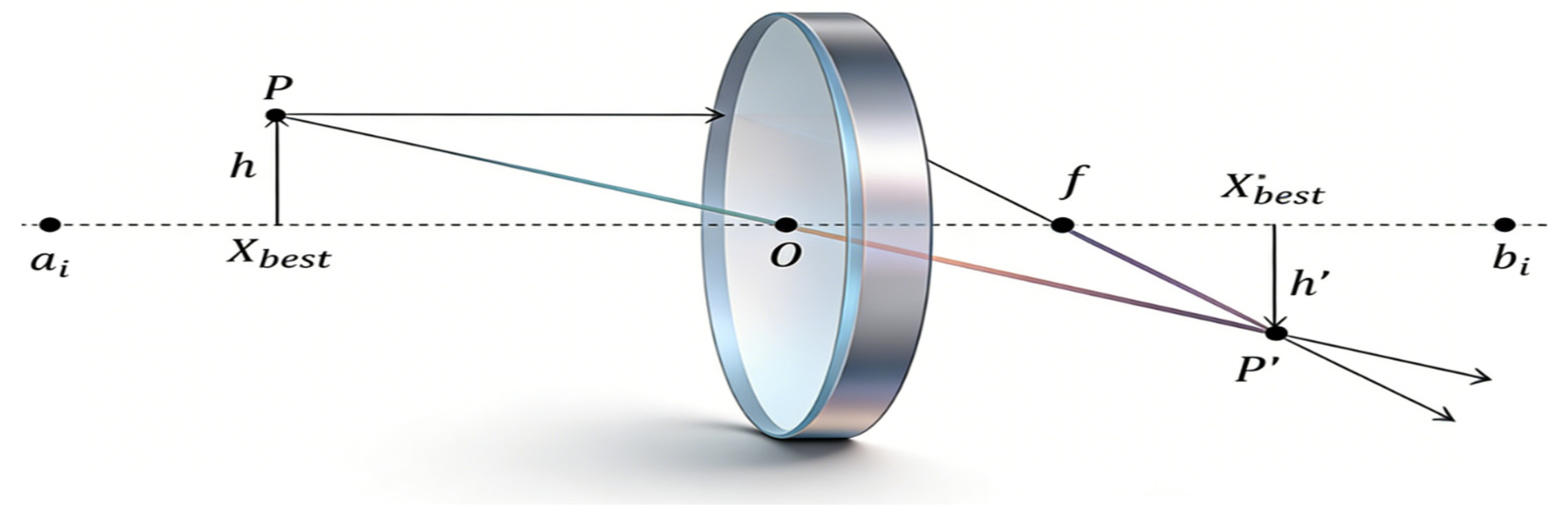
To resolve this specific flaw, RAPO employs a Kinematic Boundary Repair strategy based on convex-lens imaging. We redesign the standard OBL into a Limit Control mechanism. Instead of resetting an invalid individual, this method treats the joint limit as a “refractive interface.” By calculating a symmetrical feasible position, the algorithm “reflects” the agent back into the valid workspace. This customized correction ensures that the evolutionary information carried by the agent is preserved rather than discarded, turning a boundary violation into a valid search step.

As shown in Figure 2, convex-lens imaging follows the law of optical refraction. Where $a_i$ and $b_i$ are the upper and lower bounds of the lens imaging range, respectively, $X_{best}(t)$ is the best position, $X_{best}^{\ast }(t)$ is the opposite position of the best position, $h$ is the height of an individual, and $h^{\ast }$ is the corresponding height of the individual obtained through the lens. The focal length of the convex lens is $f$, and the center of the optical axis is O.

According to the geometric optics principle of convex-lens imaging, the direction of the light ray passing through the lens center remains unchanged. Therefore, two similar triangles are formed on the object side and the image side. Based on the properties of similar triangles, we can obtain:

$${\displaystyle \frac{(a_i+b_i)/2-X_{best}\left(t\right)}{X_{best}^{\ast }\left(t\right)-(a_i+b_i)/2}}={\displaystyle \frac{h}{h^{\ast }}}$$

(23)

Now let ${\displaystyle \frac{h}{h^{\ast }}}=n$, and by rearranging Equation (2), we obtain:

$$X_{best}^{\ast }\left(t\right)={\displaystyle \frac{(a_i+b_i)}{2}}+{\displaystyle \frac{(a_i+b_i)}{2n}}-{\displaystyle \frac{X_{best}\left(t\right)}{n}}$$

(24)

where the magnitude of $n$ is proportional to the range of the generated opposite solution. By adjusting $n$, the dynamic acceptance ability in lens opposition-based learning can be obtained.

RAPO calls a custom function for boundary handling:

$$X_{i,j}^{\prime }=\alpha \left(U_j+L_J-X_{i,j}\right)+\left(1-\alpha \right)X_{i,j}$$

(25)

Here, $\mathsf{\alpha }\in \left(\mathrm{0,1}\right)$ is the refraction coefficient, and $U_j, L_j$ are the upper and lower bounds. This formula is equivalent to a lens refraction correction. It keeps part of the individual’s original direction, so that an out-of-bounds individual is smoothly reflected back within the bounds.

Unlike simple reflection or truncation, CLOBC offers distinct practical advantages:

• Information Preservation: Instead of blindly resetting the particle, Equation (25) maps the invalid solution to a valid position based on its original trajectory. This preserves the kinetic energy of the search.
• Active Exploration: CLOBC transforms a boundary violation into an opportunity for opposition-based learning (OBL). By calculating the “refracted” position, the algorithm explores the symmetric region of the search space. This effectively turns a “failed” search step into a “probabilistic jump” that helps escape local optima.
• Dynamic Mapping: The introduction of the coefficient $\mathsf{\alpha }$ ensures that the mapping is not a rigid geometric symmetry but includes stochastic variation, further enhancing the algorithm’s robustness against periodic traps.

2.2.4. Selective Centroid Opposition-Based Learning, SOBL

Opposition-based learning (OBL), introduced by Tizhoosh in 2005 [32], is a strategy used in intelligent optimization. It is based on the observation that, within a search interval, the opposite of a current candidate can be closer to the global optimum than the candidate itself. For a point $\mathcal{X}$ in the search space [a,b], its opposite point $\tilde{\mathcal{X}}$ is defined as:

$$\tilde{\mathcal{X}}=a+b-\mathcal{X}$$

(26)

Traditional OBL uses the midpoint of the search space as the symmetry center, and it does not fully use the evolutionary information of the population. To address this, Rahnamayan et al. [33] proposed Centroid Opposition-Based Learning (COBL), which uses the centroid of the better individuals in the population as the symmetry center to better guide the search direction. However, existing COBL methods usually compute the centroid using a fixed number of individuals, and they lack dynamic adaptive ability.

This paper proposes a Selective Centroid Opposition-Based Learning (SOBL) strategy. It computes the centroid by randomly selecting different numbers of better individuals, which improves adaptability and population diversity.

(1)

Random parameter selection

In each iteration, the parameter is generated at random:

$$K=randi\left(N\right)$$

(27)

$$K\in [1,N]$$

$N$ is the population size. This random mechanism makes the centroid position dynamic across different iterations, and it avoids search stagnation caused by a fixed selection strategy.

(2)

Population ranking and centroid computation

Sort in ascending order of fitness:

$$f(\overrightarrow{X_1})\le f(\overrightarrow{X_2})\le \cdots \le f(\overrightarrow{X_N})$$

Compute the centroid of the current top $K$ individuals:

$$\overrightarrow{M}={\displaystyle \frac{1}{K}}\sum _{j=1}^K\overrightarrow{X_j}$$

(28)

$\overrightarrow{X_j}$ denotes the j-th individual after sorting. The centroid $\overrightarrow{M}$ represents the distribution center of the better solutions in the current population.

(3)

Generation of the opposite solution

Based on the centroid $\overrightarrow{M}$, generate the opposite solution for each individual:

$$\widetilde{\overrightarrow{X_i}}=2\overrightarrow{M}-\overrightarrow{X_i}$$

(29)

$$i=\mathrm{1,2},\dots \dots ,N$$

This formula shows that the opposite solution $\widetilde{\overrightarrow{X_i}}$ is symmetric to the original solution $\overrightarrow{X_i}$ with respect to the centroid $\overrightarrow{M}$. When $\overrightarrow{X_i}$ is far from $\overrightarrow{M}$, its opposite solution will be closer to $\overrightarrow{M}$, and vice versa.

(4)

Boundary handling

Apply boundary constraints to opposite solutions that exceed the search space:

$${\widetilde{\overrightarrow{X_i}}}^d=max\left(min\left({\widetilde{\overrightarrow{X_i}}}^d,u{b}_d\right),l{b}_d\right)$$

(30)

${\widetilde{\overrightarrow{X_i}}}^d$ denotes the $d$ th component of the opposite solution, and $u{b}_d$ and $l{b}_d$ are the upper and lower bounds of the $d$ th dimension, respectively.

(5)

Greedy selection

A greedy strategy is used to select the better one between the original solution and the opposite solution to update the population:

$${\overrightarrow{X}}_i^{new}=\left\{\begin{array}{c}\widetilde{\overrightarrow{X_i}}, if f(\widetilde{\overrightarrow{X_i}})<f(\overrightarrow{X_i})\\ \overrightarrow{X_i}, otherwise\end{array}\right.$$

(31)

This greedy mechanism guarantees that population quality strictly improves. Crucially, regarding diversity, SOBL outperforms classical OBL (which uses a static midpoint) and standard COBL (which relies on a fixed-size centroid). By dynamically randomizing the number of elite individuals ($K$) used to calculate the symmetry center, SOBL introduces a stochastic “jitter” to the reference point in each iteration. This fluctuation forces opposite solutions to scan diverse neighborhoods even when the population clusters. Consequently, this continuous variation in search trajectories effectively prevents the stagnation observed in fixed-strategy methods and significantly enhances the algorithm’s ability to escape local optima.

2.2.5. Algorithm Description of RAPO

The proposed RAPO algorithm introduces four improvement strategies based on the original APO. The proposed RAPO framework is not a simple stacking of strategies. Instead, it represents a systemic reconstruction of the search logic. The synergy among the four mechanisms addresses the inherent limitations of the original APO in high-dimensional and multimodal landscapes. The internal theoretical coherence is analyzed as follows.

First, DFDB reconstructs the global guidance mechanism. In the original APO, the “Aerial Flight” stage relies solely on the fitness value to select the leader. This greedy approach causes the population to collapse into local optima too quickly. DFDB introduces the Euclidean distance as a dynamic weight. It forces the algorithm to select leaders that are both high-quality and spatially distant. This mechanism transforms the search behavior from “blind following” to “dispersed exploration.” It ensures sufficient population diversity in the early stages.

Second, DEPSS reshapes the local exploitation engine. The original “underwater foraging” stage uses a simple linear contraction. This often leads to stagnation when the solution is close to the theoretical optimum. DEPSS integrates an elite pool with heavy-tailed perturbations. The elite pool acts as a memory bank to preserve historical high-quality information. The perturbations introduce multi-scale random jumps during the convergence process. This combination allows the algorithm to perform fine-grained searches while retaining the kinetic energy to escape saddle points.

Third, CLOBC and SOBL serve as the correction and recovery layer. Standard boundary handling methods simply truncate out-of-bound solutions. This results in a loss of search efficiency. CLOBC utilizes the convex-lens imaging principle to map invalid solutions back into the feasible region. This turns potential information loss into valid exploration. Furthermore, SOBL operates on the population centroid. When the swarm aggregates and stagnation occurs, SOBL generates reverse solutions based on the geometric center. This provides a secondary probability to jump out of local traps.

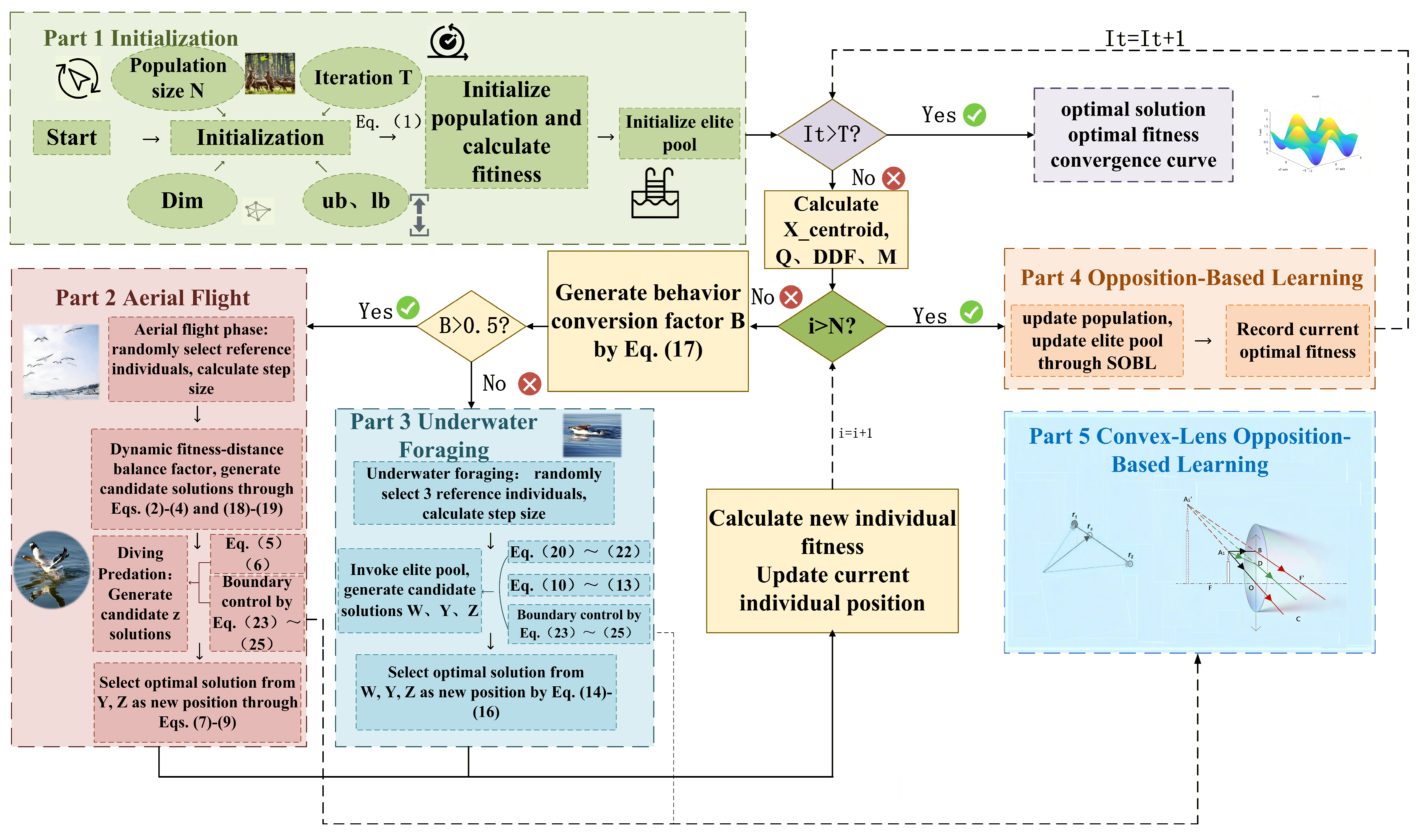
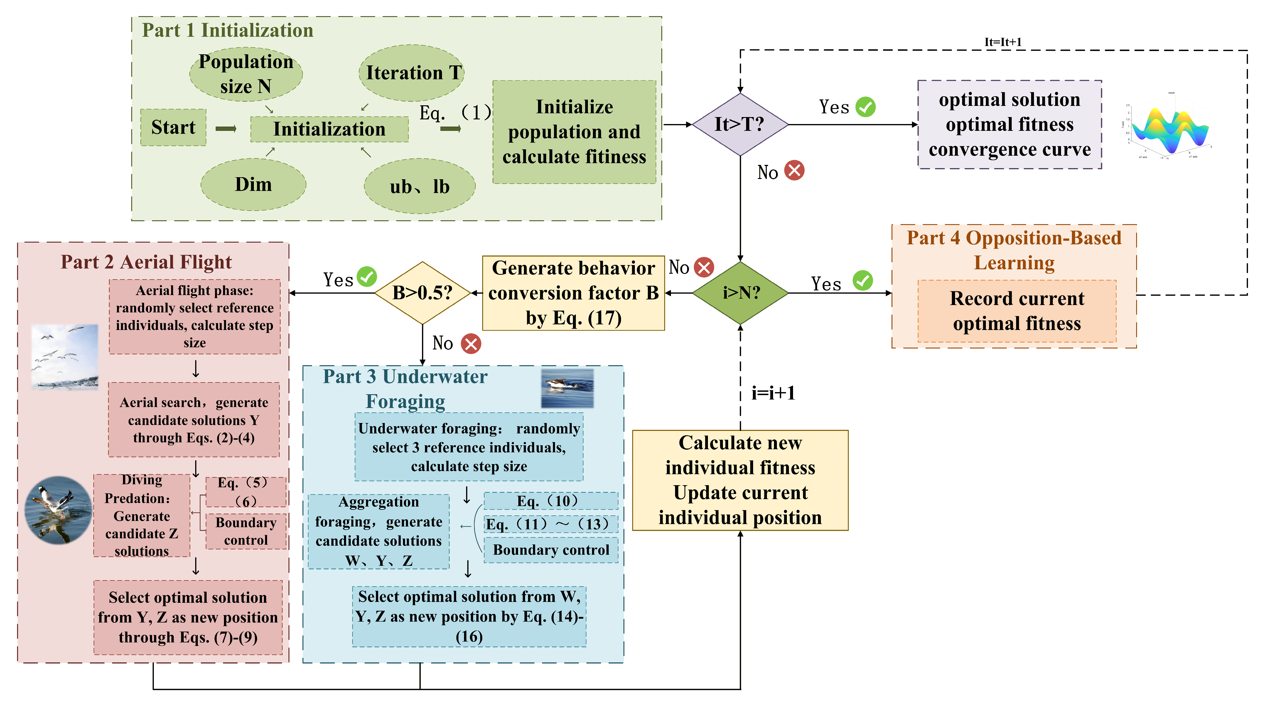
In summary, these strategies form a complementary closed-loop system. DFDB guarantees global coverage. DEPSS ensures local precision and escape capability. CLOBC and SOBL provide boundary safety and stagnation recovery. This multi-layer structure enables RAPO to handle complex optimization tasks more robustly than the single-layer logic of the original APO. The pseudocode of the RAPO algorithm is shown in Algorithm 1, and the detailed procedure of RAPO is shown in Figure 3.

Algorithm 1 Reinforced Arctic Puffin Optimization (RAPO)
	Input: Population size N, max iterations T, dimension dim, bounds [lb, ub]
	Output: Best solution X_best, best fitness f_best, convergence curve
1	Initialize population $\overrightarrow{X}$ according to Equation (1)
2	Evaluate fitness for all individuals
3	Obtain X_best and f_best
4	Initialize elite pool Elite_pool by Equation (20)
5	For  It = 1 to T do
6	Compute population centroid X_centroid
7	Calculate behavior transition factor B by Equation (17)
8	Update dynamic parameters Q, DDF, M
9	For i = 1 to N do
10	Generate random number rand ∈ [0, 1]
11	If (B > 0.5) then
12	Randomly select reference individuals, compute step1
13	Select guide individual via dFDB by Equations (18) and (19)
14	Generate aerial search candidate $\overrightarrow{Y}$ by Equations (2)–(4)
15	Generate swooping candidate $\overrightarrow{Z}$ by Equations (5) and (6)
16	Apply boundary control for $\overrightarrow{Y}$, $\overrightarrow{Z}$ by Equations (23)–(25)
17	Select best from {$\overrightarrow{Y}$, $\overrightarrow{Z}$} by Equations (7)–(9)
18	Else
19	Randomly select 3 reference individuals, compute step
20	Randomly select elite from Elite_pool
21	If (rand < 0.5) then
22	Generate candidate W by Equation (21) (t-distribution)
23	Else
24	Generate candidate W by Equation (22) (Lévy flight)
25	End if
26	Generate intensified candidate $\overrightarrow{Y}$ by Equations (11) and (12)
27	Generate evasion candidate $\overrightarrow{Z}$ by Equations (10) and (13)
28	Apply boundary control for W, $\overrightarrow{Y}$, $\overrightarrow{Z}$ by Equations (23)–(25)
29	Select best from {W, $\overrightarrow{Y}$, $\overrightarrow{Z}$} by Equations (14)–(16)
30	End if
31	If f(X_new) < f(Xi) then
32	Xi ← X_new
33	If f(X_new) < f_best then
34	X_best ← X_new, f_best ← f(X_new)
35	End if
36	End if
37	End for
38	Update population via SOBL by Equations (27)–(31)
39	Update Elite_pool
40	Record convergence curve(It) ← f_best
41	End for
42	Return X_best, f_best, curve

2.3. The Computational Complexity of the RAPO Algorithm

The computational cost of RAPO is mainly determined by two parts: (1) initializing the candidate solutions and (2) running the main steps of the algorithm. The main steps include fitness evaluation and solution updating. Overall complexity is influenced by the population size N, the maximum iterations T, and the problem dimension D. In particular, solution initialization has complexity O(N), so it scales linearly with N. Therefore, a larger population leads to a higher initialization cost.

The time complexity of the core operations in the original APO algorithm is O(T×N×D), where T is the number of iterations, N is the population size, and D is the problem dimension. Based on Equations (14)–(21), RAPO extends APO by adding four enhancements: a dynamic fitness–distance-balancing mechanism, an elite pool-based dynamic search strategy, a centroid opposition-based learning strategy, and a convex-lens-opposition boundary control strategy.

The dynamic fitness–distance balance mechanism computes the distance between each individual and the best solution and performs normalization of fitness and distance. Since this mechanism is applied to each individual, its complexity is O(N×D). The elite-pool-based dynamic search strategy maintains a dynamic archive containing four elite solutions. Maintaining the elite pool requires sorting the population, with complexity O(N log N); however, because the computational costs of the t-distribution perturbation and Lévy flight are O(N×D), when D > log N, this strategy is dominated by the O(N×D) term. The centroid opposition-based learning strategy computes the population centroid and generates opposite solutions, with complexity O(N×D). The convex-lens opposition-based boundary control strategy uses a refraction model to enforce boundary constraints by performing refraction calculations for each out-of-bounds solution, with complexity O(N×D).

Since these strategies are executed in every iteration, the time complexity of the dynamic fitness–distance balance mechanism is O(T×N×D), the elite-pool-based dynamic search strategy is O(T×N×D), the centroid opposition-based learning strategy is O(T×N×D), and the convex-lens opposition-based boundary control strategy is also O(T×N×D). In addition, the core position update process has complexity O(T×N×D), as well.

Therefore, the overall time complexity of RAPO is O(RAPO) = O(N) + O(T×N×D) + O(T×N×D) + O(T×N×D) + O(T×N×D) + O(T×N×D) = O(N) + 5×O(T×N×D) = O(T×N×D), which is consistent with the original APO algorithm. Although RAPO introduces four enhancement strategies, all of them are linear in N, T, and D and thus do not change the asymptotic order of complexity. In terms of space complexity, RAPO needs to store the population positions O(N×D), the elite pool O(D), and temporary variables O(N×D), giving a total space complexity of O(N×D), which is the same as that of the original algorithm. Overall, while maintaining the same time complexity O(T×N×D) and space complexity O(N×D) as APO, RAPO significantly improves optimization performance and convergence speed through more effective search strategies.

3. Results and Comprehensive Analysis

All simulations were conducted on a 64-bit Windows 11 system. The experiments were implemented in MATLAB R2024b and executed on a workstation equipped with an Intel Core i7-1355U CPU (1.70 GHz) and 32 GB RAM.

3.1. Test Functions and Parameter Settings

This study evaluates the proposed RAPO algorithm, using the CEC 2017 benchmark suite (Dim = 30, 50, and 100). Key information about CEC 2017 is listed in

Table 1. CEC2017 basic information.

Function	Function Name	Extreme Value	Function	Function Name	Extreme Value
F1	Shifted and Rotated Bent Cigar Function	100	F17	Hybrid Function 6 (N = 5)	1700
F3	Shifted and Rotated Zakharov Function	300	F18	Hybrid Function 6 (N = 5)	1800
F4	Shifted and Rotated Rosenbrock’s Function	400	F19	Hybrid Function 6 (N = 5)	1900
F5	Shifted and Rotated Rastrigin’s Function	500	F20	Hybrid Function 6 (N = 6)	2000
F6	Shifted and Rotated Expanded Scaffer’s F6 Function	600	F21	Composition Function 1 (N = 3)	2100
F7	Shifted and Rotated Lunacek Bi-Rastrigin Function	700	F22	Composition Function 2 (N = 3)	2200
F8	Shifted and Rotated Non-Continuous Rastrigin’s Function	800	F23	Composition Function 3 (N = 4)	2300
F9	Shifted and Rotated Lévy Function	900	F24	Composition Function 4 (N = 4)	2400
F10	Shifted and Rotated Schwefel’s Function	1000	F25	Composition Function 5 (N = 5)	2500
F11	Hybrid Function 1 (N = 3)	1100	F26	Composition Function 6 (N = 5)	2600
F12	Hybrid Function 2 (N = 3)	1200	F27	Composition Function 7 (N = 6)	2700
F13	Hybrid Function 3 (N = 3)	1300	F28	Composition Function 8 (N = 6)	2800
F14	Hybrid Function 4 (N = 4)	1400	F29	Composition Function 9 (N = 3)	2900
F15	Hybrid Function 5 (N = 4)	1500	F30	Composition Function 10 (N = 3)	3000
F16	Hybrid Function 6 (N = 4)	1600

. The benchmark set includes four categories of functions: unimodal, multimodal, hybrid, and composition. These categories are intended to test performance and applicability in a broad and systematic way. They also offer a standard framework to examine scalability, which helps us assess how RAPO performs across different problem types and dimensions.

3.2. Comparison with Other Algorithms and Parameter Settings

The performance of the RAPO algorithm is systematically compared against nine well-known algorithms. These are categorized into three distinct groups for a structured analysis.

High citation algorithms: These include Particle Swarm Optimization (PSO) [25], the Grey Wolf Optimizer (GWO) [12], and the Whale Optimization Algorithm (WOA) [14].

Latest advanced algorithms: This includes the Runge–Kutta Method-based Optimizer (RUN) [17], Newton–Raphson-Based Optimizer (NRBO) [18], and Atlantic Puffin Optimization (APO) [26]. This includes the Black-winged Kite Algorithm (BKA) [16], Secretary Bird Optimization Algorithm (SBOA) [15], and Chinese Pangolin Optimizer (CPO) [20].

Table 2. The parameter settings of the comparison algorithms.

Algorithms	Parameter	Value
PSO	Vmax, w, c1, c2	0.15, 0.8, 2, 2
GWO	α	[0, 2]
WOA	b	1
RUN	SF, γ, EXP	0.5, 4, 5
BKA	P, n	0.9, 0.05
SBOA	beta	0.5
NRBO	DF, Flag	0.6, 1
CPO	T, alpha, Tf	2, 0.2, 0.8
APO	F, beta	0.5, 1.5
RAPO	alpha	0.5

lists the parameter settings for the nine algorithms. Each algorithm was executed in 30 independent runs. In every run, the maximum number of iterations was set to 500, and the population size was fixed at 30. The search bounds were set to −100 (lower) and 100 (upper). We report the mean (Ave) and standard deviation (Std) of the results. For clear comparison, the best value in each case is shown in bold, indicating the top-performing algorithm under these test settings.

3.3. Quantitative Evaluation

RAPO is evaluated on the CEC 2017 benchmark suite. All algorithms follow the same experimental settings: population size = 30, maximum iterations = 500, and 30 independent runs. The numerical results are summarized in Tables S1–S3 in the Supplementary Materials, reporting the mean (Ave) and standard deviation (Std) for each competitor; the best values are highlighted in bold. The first-row metric (W|T|L) counts the number of wins, ties, and losses over all functions, and the conclusions are supported by statistical tests to demonstrate RAPO’s performance advantages.

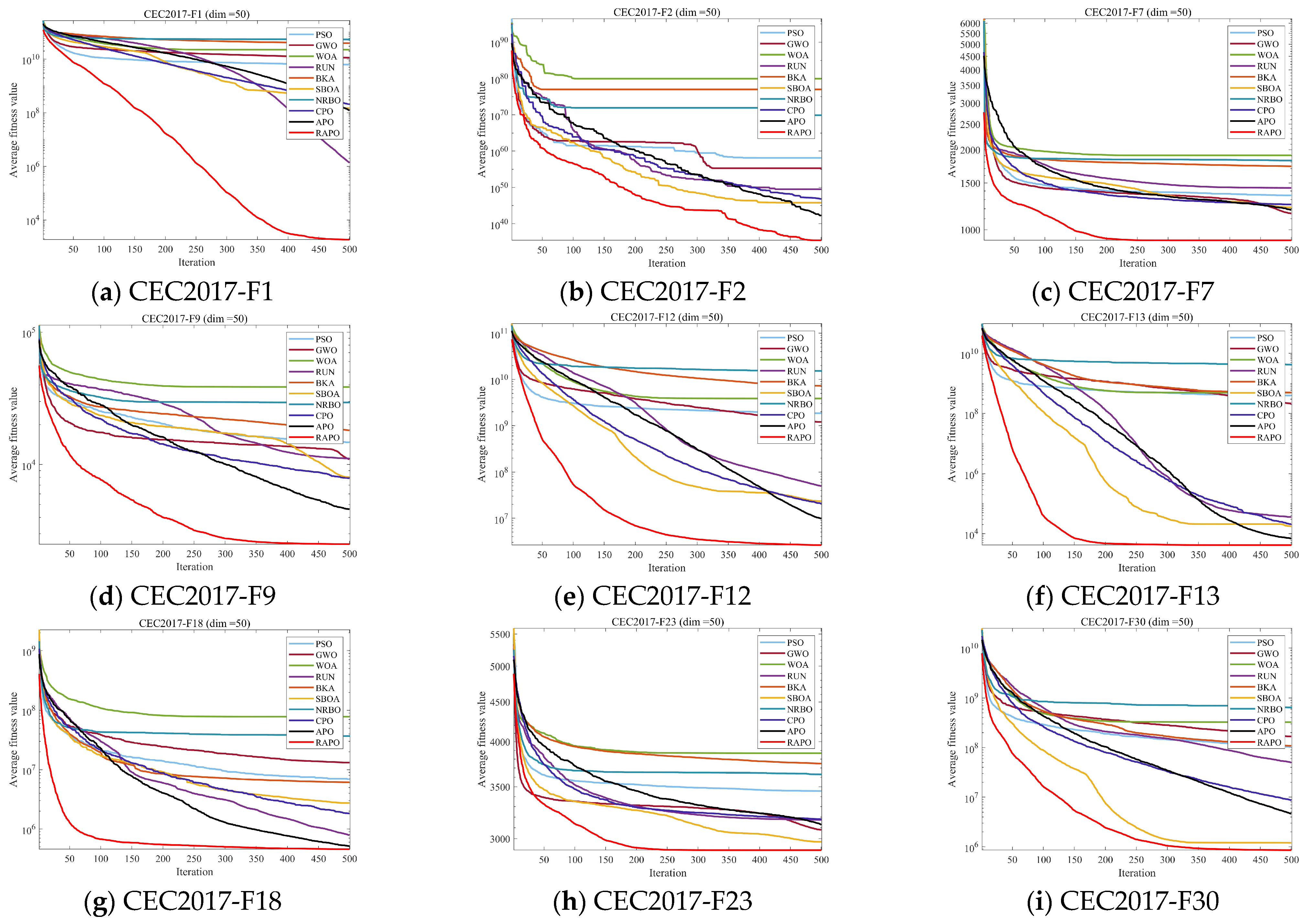
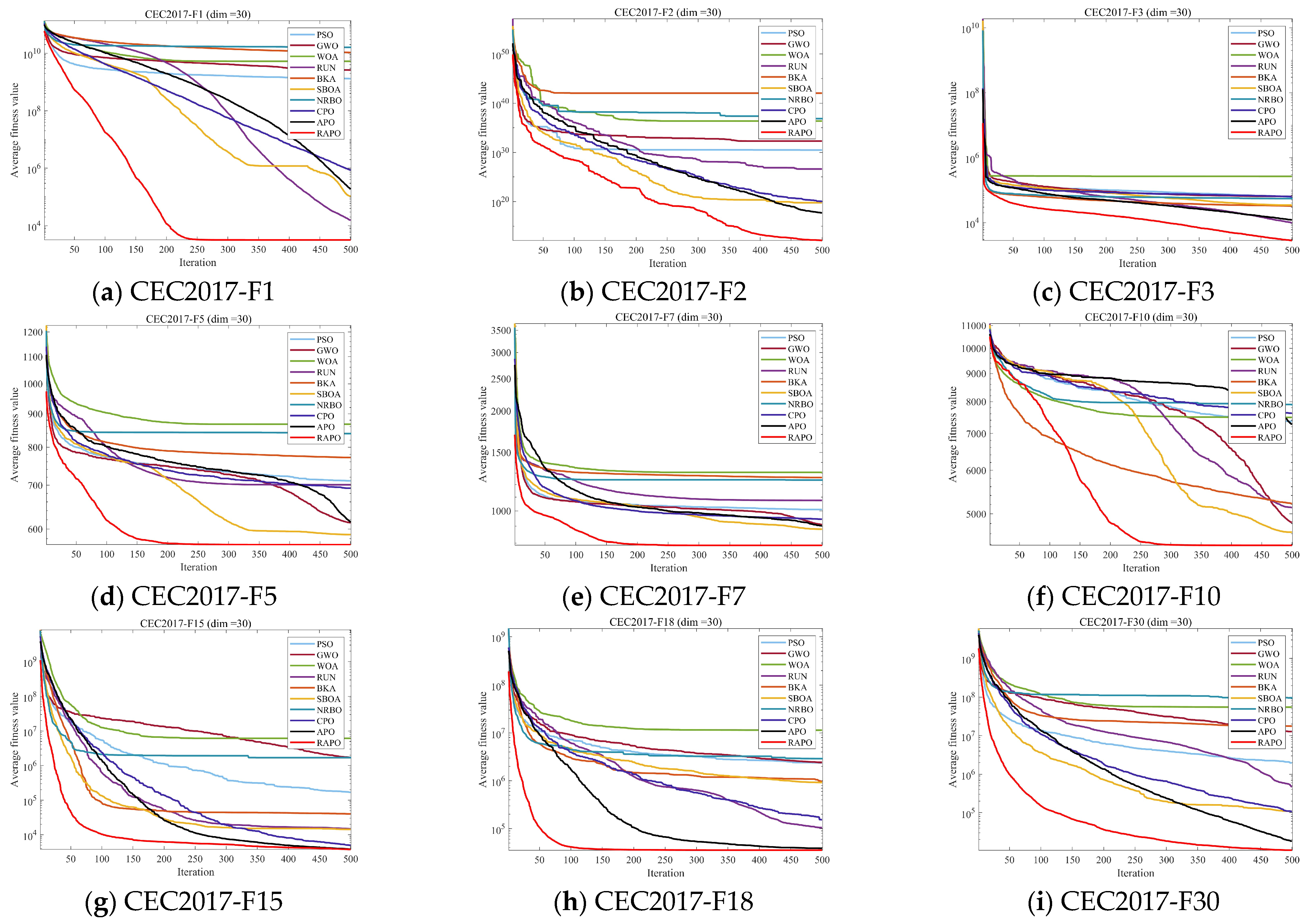
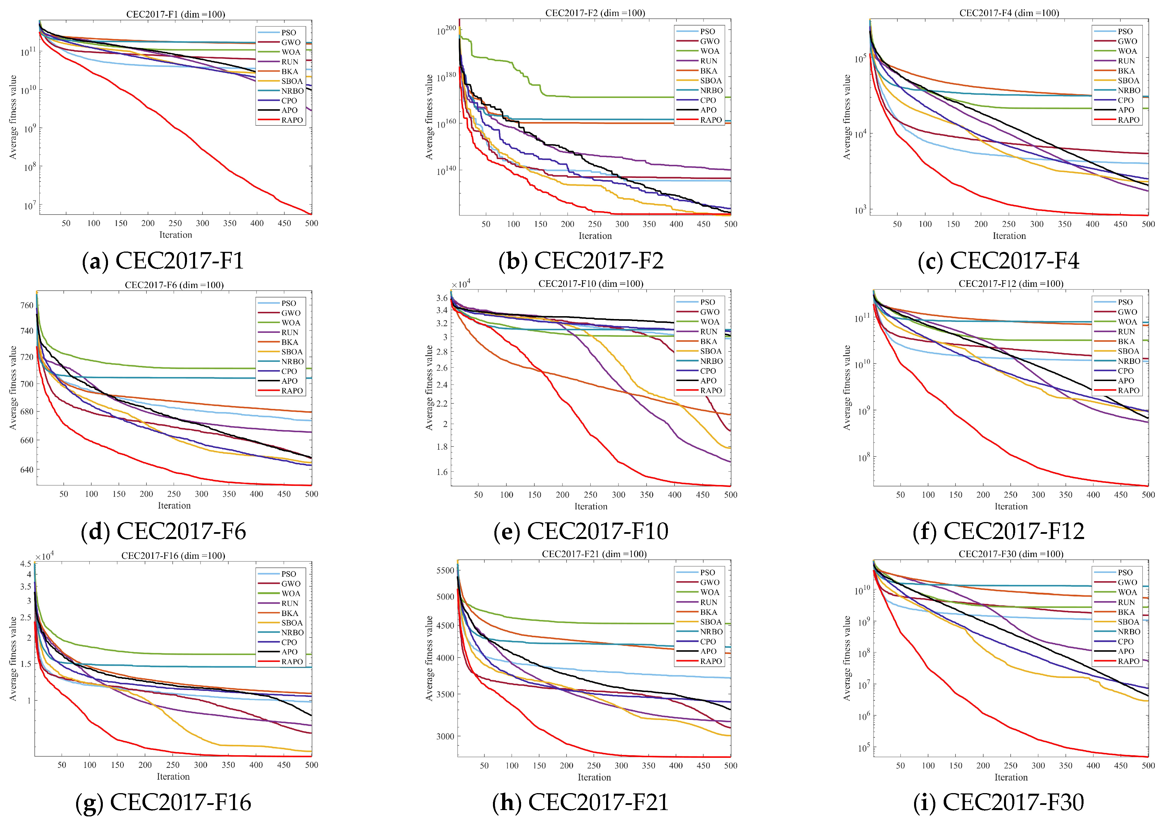
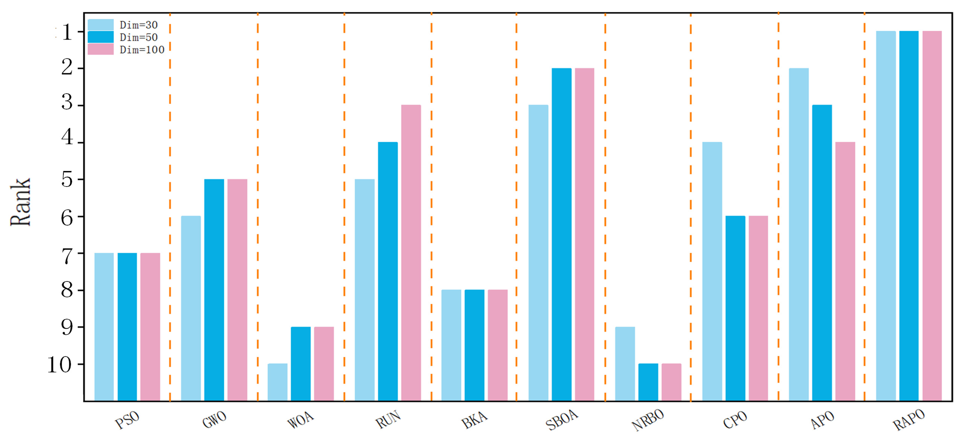
Figure 4, Figure 5 and Figure 6 show the convergence curves to compare search progress and efficiency across iterations. In addition, Figure 7 presents the average Friedman ranks on the 30D, 50D, and 100D test sets. Overall, the results confirm the robustness and adaptability of RAPO under different optimization settings.

3.3.1. Assessing Performance with CEC 2017 Test Suite (30 Dim)

This section assesses RAPO on the CEC 2017 benchmark suite. The first set of experiments was performed in a 30-dimensional search space. The corresponding results are presented in Table S1, where the best method among the ten competing algorithms is marked in bold.

On functions F1, F2, F3, F15, F18, and F30, RAPO achieves a much better mean performance than the other algorithms, showing higher solution accuracy. This indicates that RAPO has a clear accuracy advantage when dealing with complex objective functions. The results also show that RAPO is better at escaping local optima and can find better global solutions in very difficult search spaces. In addition, RAPO has a smaller standard deviation on most test functions, which shows better convergence stability and robustness. This means that across multiple independent runs, RAPO usually converges to similar solutions with less variation, giving more consistent and reliable performance.

In the performance evaluation, RAPO achieves (W|T|L) = (21|9|0). This means that among the 30 test functions, it obtains the best result on 21 functions, ties with other algorithms on nine functions, and is not the worst on any function. This result clearly shows that RAPO outperforms the comparison algorithms in most cases and does not show an obvious disadvantage in any specific case. The Friedman test further supports this conclusion. RAPO ranks first with an average Friedman rank of 1.3. This indicates that RAPO not only performs well on individual functions but also shows balanced overall optimization ability.

Figure 4 illustrates the convergence behavior of all algorithms in the 30-dimensional space. We divide the test functions into different types to analyze the search progress. For example, Figure 4a,b show the results for unimodal functions. Here, RAPO demonstrates a rapid downward trend. Figure 4d–i display the results for complex multimodal and hybrid functions. In these cases, RAPO effectively avoids local optima and reaches lower fitness values. These curves represent the average performance over 30 independent runs. This averaging process effectively reduces the impact of random variation. This rapid convergence is mainly attributed to the CLOBC strategy introduced in the initialization and update phases. By utilizing opposition-based learning, the algorithm can search the solution space more broadly and guide the population toward the promising region more quickly than random search. In particular, for complex hybrid functions, RAPO shows a faster and more stable decreasing trend, reflecting its stronger global exploration ability when solving difficult problems. Overall, these results clearly demonstrate the effectiveness and superiority of RAPO as an optimization tool.

3.3.2. Assessing Performance with CEC 2017 Test Suite (50 Dim)

In this section, to further evaluate the performance of RAPO, we extend the tests to a 50-dimensional high-dimensional and complex setting. The results are shown in Table S2, where the best-performing algorithm among the ten candidate algorithms is highlighted in bold. The results show that when the dimension increases to 50, RAPO still remains leading on many tests. Compared with the other algorithms, RAPO achieves clearly better accuracy, which shows its strong global search ability when dealing with high-dimensional nonconvex objective functions. The average Friedman test result over all test functions ranks RAPO first overall, and it is within the top two in all experiments, outperforming other advanced algorithms in the same category.

Figure 5 details the convergence curves for the 50-dimensional setting. The subfigures present results across various function types. Specifically, Figure 5a–c confirm the fast convergence speed of RAPO on simple functions. Furthermore, Figure 5d–i highlight its strong global search ability on highly complex functions. RAPO consistently achieves better accuracy than the competing algorithms across all these specific test cases. Across the tested functions and optimization settings, RAPO demonstrates excellent overall performance and robustness, which further confirms its effectiveness for solving this type of problem.

3.3.3. Assessing Performance with CEC 2017 Test Suite (100 Dim)

Extending the assessment to 100 dimensions, RAPO achieves (W|T|L) = (28|2|0). The detailed results are reported in Table S3, surpassing its performance in the 30D and 50D cases. This scalability indicates that RAPO maintains high accuracy even as the search space complexity increases exponentially. Beyond the numerical dominance, the performance variations across different function categories reveal how the proposed strategies specifically enhance the optimization process in high-dimensional spaces. For unimodal functions (F1, F3), the rapid convergence is primarily attributed to the CLOBC and SOBL strategies, which effectively shrink the search space boundaries and utilize opposition-based learning to accelerate exploitation near the global optimum. In contrast, for multimodal functions (F4–F10) riddled with local optima, the DEPSS plays a critical role by integrating Lévy flight and t-distribution perturbations to maintain population diversity and escape local basins of attraction. Furthermore, in the most complex hybrid and composition functions (F11–F30), the superior performance validates the effectiveness of the DFDB mechanism, which adaptively regulates the trade-off between exploration and exploitation based on real-time population distribution, ensuring robustness even when landscape characteristics change abruptly. The lower standard deviation observed in functions like F8, F21, F25, and F28 confirms that these mechanisms work synergistically to provide consistent stability across independent runs, as further illustrated by the convergence curves in Figure 6.

The superior performance of RAPO on the CEC2017 benchmark suite provides a theoretical guarantee for its application in robotic trajectory planning. Specifically:

• Handling High Dimensions: The algorithm’s dominance in 50D and 100D cases is crucial. In trajectory planning, optimizing cubic B-spline paths for a 6-DOF manipulator involves optimizing dozens of control points simultaneously. RAPO’s ability to maintain high accuracy in high-dimensional spaces ensures it can generate smooth and precise trajectories.
• Escaping Local Optima: The strong performance on hybrid and composition functions demonstrates RAPO’s ability to navigate complex, multimodal landscapes. This directly translates to the ability to avoid local minima caused by dense obstacles (branches and trunks) in the orchard environment.
• Stability: The low standard deviation observed across independent runs indicates high reliability. For agricultural robots, this means RAPO can consistently generate safe and feasible paths under varying initial conditions, which is essential for continuous harvesting operations.

3.4. Ablation Experiment

Strategy combination plays a crucial role in improving algorithm performance. To systematically evaluate the contribution of the four proposed enhancement mechanisms to RAPO, this study designed two types of mechanism ablation experiments, namely progressive addition and progressive removal. In the progressive addition experiment, each strategy was introduced into the basic APO algorithm in turn to observe the resulting performance improvement. In the progressive removal experiment, one mechanism was removed from the complete RAPO at a time to analyze its importance.

Table 3. Various RAPO variants with four strategies.

Algorithms	DFDB	DEPSS	CLOBC	SOBL
APO	0	0	0	0
DFAPO	1	0	0	0
DEAPO	0	1	0	0
CAPO	0	0	1	0
SAPO	0	0	0	1
DFDECAPO	1	1	1	0
DFDESAPO	1	1	0	1
DFCSAPO	1	0	1	1
DECSAPO	0	1	1	1
RAPO	1	1	1	1

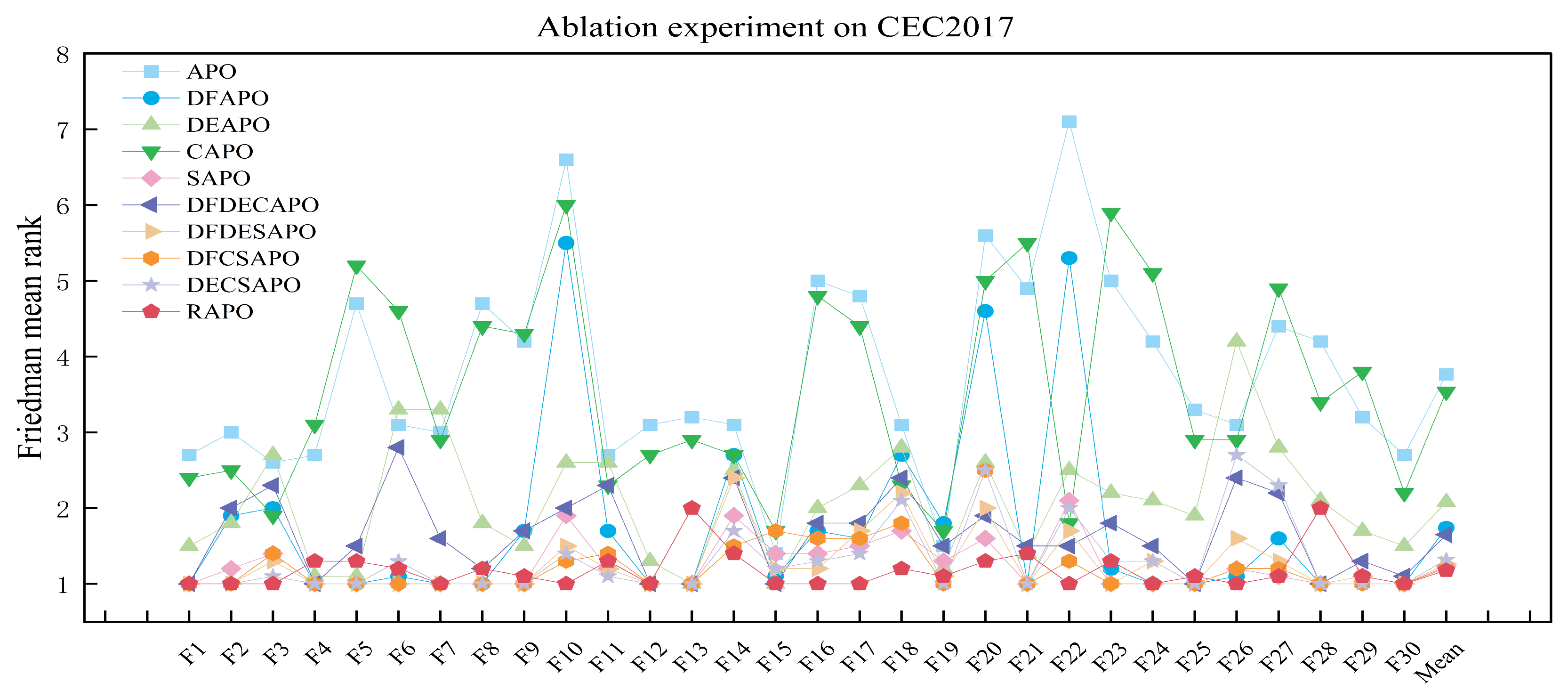
lists the configurations of each strategy combination, where “1” indicates enabled and “0” indicates disabled. Figure 8, showing the ablation experiment on CEC2017 (Dim = 100), presents the average ranks of ten strategy combinations based on the Friedman test on the CEC2017 test suite with Dim = 100. The results indicate that RAPO, which integrates all four mechanisms, achieves the best performance on most functions, with an average rank of 1.18, outperforming all other combinations. In contrast, the original APO exhibits moderate overall performance, with an average rank close to 4. SAPO, which includes only the SOBL strategy, achieves the best performance among the single strategy variants with an average rank of 1.3, indicating that centroid-based opposition learning, SOBL, is the core driving strategy for performance improvement. Notably, incorporating any single mechanism alone, such as DFAPO, DEAPO, CAPO, or SAPO, yields limited improvement and remains clearly inferior to multi-strategy fusion models, suggesting that an individual mechanism cannot fully exploit the algorithm potential. Meanwhile, RAPO consistently ranks first on representative functions, such as F3, F12, and F25, demonstrating excellent adaptability and robustness on multimodal and composite problems. Overall, the ablation experiments systematically verify the effectiveness and necessity of each strategy in the RAPO algorithm. SOBL acts as the core driver, DFDB provides a dynamic balancing mechanism, DEPSS enhances local search capability, and CLOBC improves boundary handling. The synergistic effect of the four strategies enables RAPO to maintain strong exploration while achieving efficient convergence and superior solution quality.

4. Application of the PAPO in Trajectory Planning for a Fruit-Picking Robotic Arm

This section investigates the application of the RAPO algorithm in practical engineering by establishing a trajectory planning framework for a fruit-picking robotic arm. Fruit-picking tasks typically involve unstructured environments with narrow spaces and dense obstacles, requiring the end-effector to approach targets smoothly while avoiding branches. To address this, we first establish the kinematic model of the manipulator and the mathematical representation of the obstacle environment. To specifically validate the mathematical performance of the proposed algorithm, the trajectory planning is formulated as a constrained optimization problem that balances path length, motion smoothness, and safety. Finally, the proposed RAPO algorithm is employed to solve for the optimal trajectory.

4.1. System Modeling

4.1.1. Manipulator Kinematics

Before detailing the trajectory optimization cost functions, it is essential to define the physical properties of the robotic arm and the operating environment. The simulation employs a 5-DOF serial manipulator designed for agricultural picking tasks. The forward kinematics are established using the Modified Denavit–Hartenberg (MDH) convention. The transformation matrix between adjacent links is defined by four parameters: link length ($a_{i-1}$), link twist (${\alpha }_{i-1}$), link offset ($d_i$), and joint angle (${\theta }_i$). Based on the physical structure, the specific D-H parameters are listed in

Table 4. Modified D-H parameters of the 5-DOF manipulator.

Joint (i)	${\mathit{\alpha }}_{\mathit{i}-1}$ (rad)	${\mathit{a}}_{\mathit{i}-1}$ (mm)	${\mathit{d}}_{\mathit{i}}$ (mm)	${\mathit{\theta }}_{\mathit{i}}$ (rad)	Range (rad)
1	0	0	0	0	($-\pi ,\pi$)
2	−$\pi /2$	0	0	0	($-\pi ,\pi$)
3	0	$L_2$	0	0	($-\pi ,\pi$)
4	0	$L_3$	0	0	($-\pi ,\pi$)
5	−$\pi /2$	0	0	0	($-\pi ,\pi$)
End-Effector	0	0	$L_4$	0	($-\pi ,\pi$)

.

The robot is mounted on a base with a height of $L_1=106.45 \mathrm{m}$. The parameters correspond to $L_2=101.985 \mathrm{m}\mathrm{m}$, $L_3=95.05 \mathrm{m}\mathrm{m}$, and $L_4=107.43 \mathrm{m}\mathrm{m}$.

The position of the end-effector is derived from the homogeneous transformation matrix. In this study, trajectory planning is performed in the Cartesian workspace, and inverse kinematics (IKs) are used to verify that the generated path points lie within the reachable workspace.

4.1.2. Obstacle Avoidance Encoding

To ensure safety in the orchard environment, obstacles (such as tree branches and trunks) are modeled as spheres to simplify collision detection. This assumption does not fully reflect real agricultural constraints but provides an efficient mathematical basis for algorithmic validation and collision detection. Five obstacles set as $\Omega =\left\{O_1,O_2,O_3,\dots ,O_k\right\}$ are defined, where each obstacle $O_k$ is characterized by its center coordinate $C_k$ and radius $r_k$.

The collision avoidance constraint is encoded as a hard constraint. For any point $P_i$ on the planned trajectory, the Euclidean distance to the $k$-th obstacle center must satisfy:

$$\parallel P_i-C_k\parallel >r_k+r_{safe}$$

(32)

where is $r_{safe}$ a safety margin. If a candidate solution violates this condition (the path intersects with any obstacle sphere), it is assigned an infinite cost penalty. This mechanism ensures that the RAPO algorithm automatically discards infeasible paths.

4.2. Trajectory Planning for the Robotic-Arm Model

4.2.1. Path Length Cost

Path length is closely related to the travel distance and energy consumption during the picking process. In general, under the prerequisites of obstacle avoidance and reachability, a shorter path implies lower actuator output and higher operational efficiency. This is especially important in repetitive picking scenarios, where it can significantly reduce the energy consumption and execution time per task.

To quantify this cost, this study uses the sum of Euclidean distances between adjacent discrete path points to represent the path length in three-dimensional space. For a three-dimensional trajectory containing N points, the path length cost is defined as:

$$L={\sum }_{i=1}^{N-1}\sqrt{{(x_{i+1}-x_i)}^2+{(y_{i+1}-y_i)}^2+{(z_{i+1}-z_i)}^2}$$

(33)

The discrete points form a spatial sequence of the robot end-effector in time order. N is the number of path points, and $(x_i, y_i, z_i)$ and $(x_{i+1}, y_{i+1}, z_{i+1})$ are two adjacent points on the path. A smaller value of this cost term indicates a more compact overall trajectory, corresponding to a shorter travel distance and potentially lower energy consumption.

4.2.2. Turning Angle Cost

When a fruit-picking robotic arm moves in an environment with dense branches and leaves, overly sharp turns in the trajectory can lead to large joint accelerations and impacts, increasing end-effector vibration and the risk of collision, and thus reducing picking stability. To constrain the geometric smoothness of the trajectory, this paper introduces a turning angle cost C to measure the degree of direction change between adjacent path segments. It is defined as:

$$C=\sum _{i=1}^{N-1}(\mathit{cos}({\displaystyle \frac{\pi }{2}})-{\displaystyle \frac{v_i·v_{i+1}}{\left|\right|v_i\left|\right| \left|\right|v_{i+1}\left|\right|}})$$

(34)

$$v_i=(d{x}_i, d{y}_i, d{z}_i)$$

Here, $v_i$ and $v_{i+1}$ denote the displacement vectors of two consecutive segments on the path. A smaller value for this term indicates a gentler turning of the trajectory, which better meets the requirements of a smooth approach and safe motion in fruit-picking tasks.

4.2.3. Height Variation Cost

In fruit-picking scenarios, the robotic arm often needs to move between different height levels to avoid branches, leaves, supports, or nearby equipment. If the trajectory shows large fluctuations in the vertical direction, it may increase the probability of collisions with surrounding objects and also cause unnecessary energy consumption and control burden. Therefore, this paper uses a height variation cost H to measure the vertical fluctuation of the trajectory. It is expressed as the sum of absolute deviations of the heights of all path points from the average height:

$$H=\sum _{i=1}^N|z_i-\overline{z}|$$

(35)

$\overline{z}$ denotes the average value. A smaller value for this term indicates that the trajectory is more stable in the height direction, which helps reduce collision risk and improves the controllability of the picking motion.

4.2.4. Comprehensive Performance Metric for Trajectory Planning

To jointly consider the requirements of path length, turning angle variation, and height fluctuation, this paper combines the three cost terms through the weight coefficients ${\omega }_1,{\omega }_2,{\omega }_3$, and constructs an overall objective function F for trajectory planning for the fruit-picking robotic arm. This objective is used to evaluate the overall quality of candidate paths and serves as the optimization target of the proposed improved algorithm:

$$F={\omega }_{1}L+{\omega }_{2}C+{\omega }_{3}H$$

(36)

${\omega }_1$, ${\omega }_2, {\omega }_3$ denote the weights of the corresponding cost terms, which are used to balance the relative importance of efficiency, represented by path length, smoothness, represented by turning angle, and vertical safety margin, represented by height variation. The optimization aims to minimize F and, under feasibility and obstacle avoidance constraints, obtain a picking trajectory with better overall performance. In this paper, the weight values used in the overall loss function for fitness evaluation are set to $1/3$ for ${\omega }_1$, ${\omega }_2, {\omega }_3$.

4.3. Simulation and Analysis of Robotic Arm Trajectory Planning

4.3.1. Algorithm Application and Simulation Experiments

To verify the effectiveness of the RAPO algorithm in robotic arm trajectory planning, this experiment applies it to an optimal path planning problem in three-dimensional space. Based on the three loss functions introduced in Section 4.2, and under the condition that the planned path does not collide with obstacles and does not pass through them, the algorithm is used to search for the path solution with the minimum overall loss.

To comprehensively evaluate the performance of RAPO on the path planning problem, CPO, NRBO, SBOA, BKA, RUN, WOA, GWO, PSO, and the original APO are also applied to the same problem for comparison.

Regarding the experimental settings, the start point of the path is set to (−150, −200, −150), and the end point is set to (300, 180, 200). The coordinates of the five obstacles are (−100, −100, 0), (−50, 0, −100), (200, 30, 100), (200, 200, 200), and (50, 100, 0), with the unit in mm. The population size is set to N = 30, and the maximum number of iterations is T = 500. To ensure fairness, the parameters of the comparison algorithms are kept consistent with those in Section 3.2.

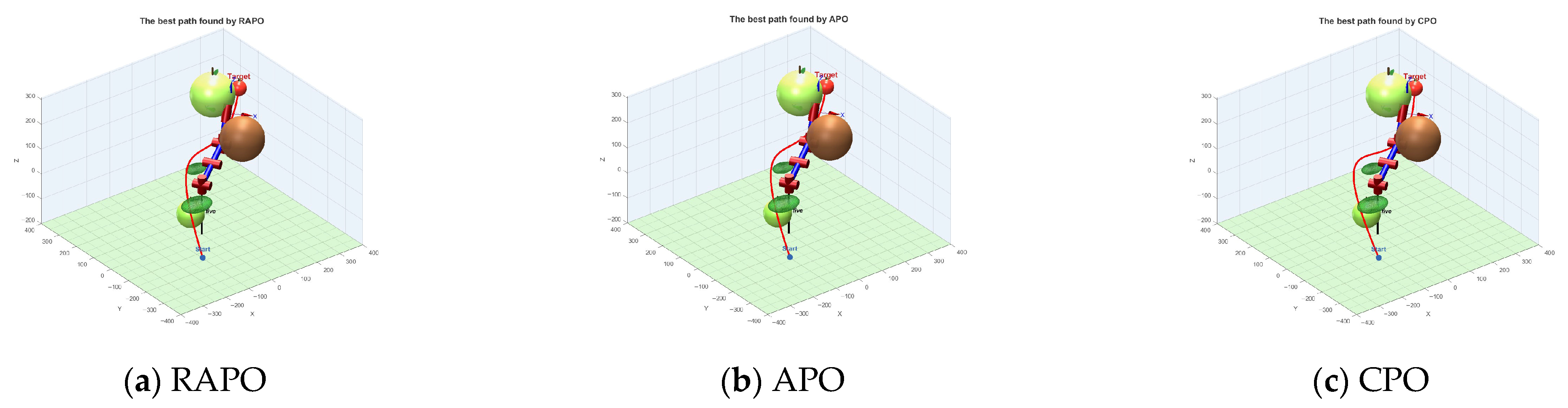
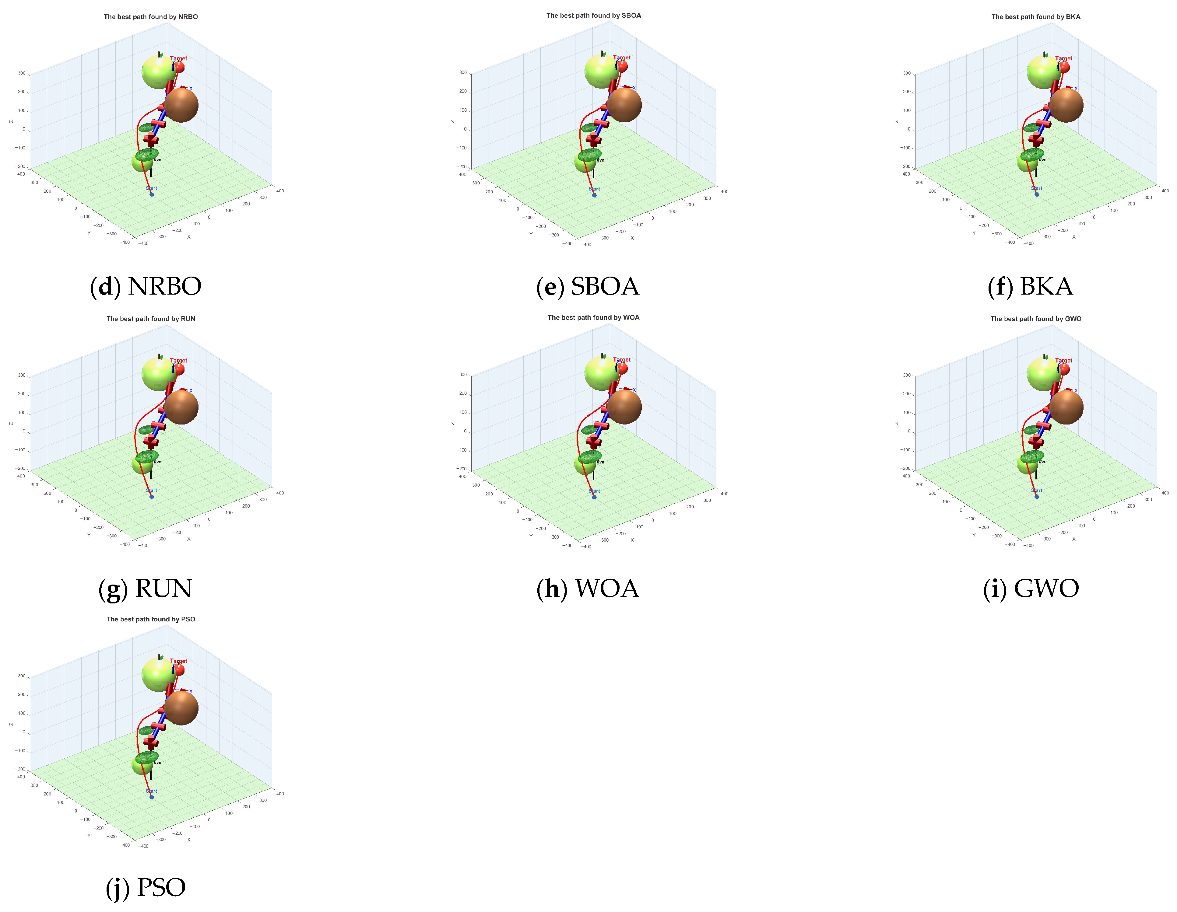
Figure 9 presents the optimal 3D trajectory planning results for each algorithm. We evaluate these paths under strict obstacle avoidance constraints. The red curve in each subfigure denotes the generated path. This integrated simulation analysis highlights the effectiveness of RAPO for path planning in complex environments and its advantages over other algorithms.

4.3.2. Simulation Results Analysis

From the paths generated by different algorithms in Figure 9, Figure 9a shows the smooth and short path generated by RAPO. Figure 9c,h,i show that the paths produced by CPO, WOA, and GWO are relatively long, which increases energy consumption, and their turning angles are overly sharp, leading to abrupt turns or large accelerations of the robotic arm and thus posing potential safety hazards. As shown in Figure 9b,g, the paths generated by RUN and APO exhibit slightly larger height variations, which increases the risk of collision with obstacles. The trajectories obtained by BKA, NRBO, SBOA, and PSO are relatively smooth and therefore safer; however, compared with RAPO, they have longer path lengths and higher energy consumption. Among the nine competing algorithms, RAPO not only yields a smoother path with smaller height variations but also achieves a notable reduction in path length, leading to favorable performance in both safety and energy consumption.

Under the same test conditions, 30 independent simulation runs were conducted for each of the ten algorithms. The overall loss values were statistically analyzed, as reported in

Table 5. Statistical results of robot-arm trajectory planning.

Algorithm	Worst Cost	Best Cost	Average Cost	Median	Standard Deviation	Wilcoxon (+/=/−)	FriedmanValue	FriedmanRank
RAPO	2.203460 × 102	2.158731 × 102	2.185801 × 102	2.184414 × 102	1.1179 × 100	=	1.000	1
APO	2.205533 × 102	2.205533 × 102	2.205533 × 102	2.205533 × 102	6.8204 × 10−14	+	5.733	6
CPO	2.205660 × 102	2.205533 × 102	2.205553 × 102	2.205538 × 102	3.3479 × 10−3	+	9.600	10
NRBO	2.205533 × 102	2.205533 × 102	2.205533 × 102	2.205533 × 102	9.2474 × 10−14	+	3.450	4
SBOA	2.205533 × 102	2.205533 × 102	2.205533 × 102	2.205533 × 102	1.4386 × 10−13	+	2.983	2
BKA	2.205533 × 102	2.205533 × 102	2.205533 × 102	2.205533 × 102	1.4559 × 10−13	+	3.133	3
RUN	2.205533 × 102	2.205533 × 102	2.205533 × 102	2.205533 × 102	1.6342 × 10−12	+	7.500	7
WOA	2.205642 × 102	2.205533 × 102	2.205542 × 102	2.205533 × 102	2.3572 × 10−3	+	7.817	8
GWO	2.205535 × 102	2.205533 × 102	2.205533 × 102	2.205533 × 102	4.8707 × 10−5	+	8.900	9
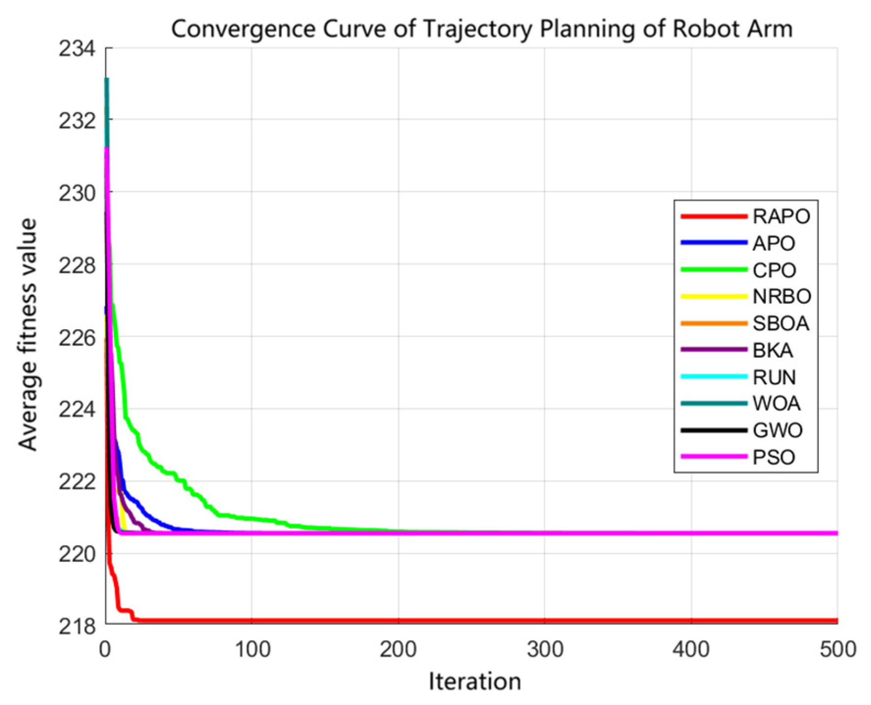
PSO	2.205533 × 102	2.205533 × 102	2.205533 × 102	2.205533 × 102	5.3303 × 10−14	+	4.883	5

, and the average convergence curves are shown in Figure 10.

As shown in Table 5, RAPO achieves the best results in terms of the best cost, worst cost, mean cost, and median cost. While most algorithms converge to local optima, RAPO identifies better solutions, indicating stronger global search capability and an improved ability to escape local optima. Although the standard deviation of RAPO (1.18) is larger than that of other algorithms, this mainly reflects enhanced global exploration rather than instability. In contrast, the extremely low standard deviations of other methods are largely attributable to premature convergence to local optima. Notably, in 30 independent runs, even the worst cost obtained by RAPO is better than the average cost of the other algorithms, demonstrating its robustness. The Wilcoxon rank sum test further indicates that RAPO achieves statistically significant performance improvements over the other nine algorithms. In the Friedman ranking, RAPO ranks first, confirming its superior performance.

From the average convergence curves in Figure 10, RAPO converges quickly and reaches the vicinity of the optimal solution within approximately the first 30 iterations. Except for CPO, the other eight algorithms also show fast convergence; for example, PSO and GWO converge even faster. However, the key difference is that RAPO converges to the global optimum rather than a local optimum. While maintaining a high convergence speed, RAPO effectively avoids premature convergence and achieves a favorable balance between convergence speed and path quality. This balance is particularly valuable in robotic arm planning, as it can substantially improve safety and reduce energy consumption in practical applications. Overall, RAPO demonstrates outstanding performance in addressing robotic arm trajectory planning problems.

5. Discussion

The results in Section 4.2 indicate that RAPO outperforms the other nine algorithms in robotic arm trajectory planning. This section further investigates the main factors behind RAPO’s performance gains for this task.

The experimental results consistently show that RAPO is better than the other competing algorithms. RAPO achieved the lowest overall path cost (218.5), which is clearly better than the local optimal solutions of other algorithms (220.55). This means RAPO can plan a motion trajectory for the robotic arm that is shorter, smoother, and uses less energy. More importantly, RAPO shows very fast convergence and reaches near the global optimum within 30 iterations, which is very important for real-time robotic arm path planning. In addition, RAPO keeps only small fluctuations during the whole optimization process, which shows high solution quality and strong robustness, and ensures stable and reliable robotic arm motion. The convergence curve comparison and the path quality evaluation both show that RAPO is the best-performing algorithm. It can effectively solve the multi-objective optimization problem in robotic arm trajectory planning, and it highlights RAPO’s excellent and reliable performance in picking robot applications.

RAPO’s strong performance can be mainly explained by four key integrated enhancement strategies: DFDB, DEPSS, CLOBC, and SOBL. The DFDB strategy adjusts the search behavior through adaptive weight tuning. In the early stage of optimization, it focuses on population diversity for wide exploration. In the later stage, it shifts to fitness priority to strengthen exploitation. This adaptive mechanism effectively prevents early convergence into local optima after 50 iterations. It allows RAPO to escape local traps and converge to the global optimum (218.5) within 30 iterations. The DEPSS strategy maintains a dynamic pool of four high-quality solutions, including the global best, the second best, the third best, and the mean of the top 50 percent. It guides the search process using t-distribution perturbation and the Lévy flight. This strategy plays a key role in keeping population diversity and avoiding local optima. The CLOBC strategy uses a refraction model to handle boundary constraints. When a solution goes out of bounds, it performs “refraction” instead of simple reflection. It keeps the original search information and also adds an opposite learning mechanism. This strategy, together with selective opposite learning based on the elite mean, improves solution feasibility while also improving path smoothness and energy efficiency. The SOBL strategy uses the population centroid as a reference point for opposite learning. It computes the geometric center of the current population and generates opposite solutions relative to the centroid. In robotic arm trajectory planning, the SOBL strategy explores new joint angle configurations in the region opposite to the centroid, which effectively expands the search range in joint space. This mechanism is especially important in the middle stage of robotic arm trajectory optimization, and it helps the algorithm escape local optimal regions.

These four strategies work together, enabling RAPO to achieve excellent performance in robotic arm trajectory planning. RAPO achieves fast global positioning in the first 30 iterations and quickly finds high-quality robotic arm motion trajectories. In the later iterations, it continues fine optimization and finally obtains a shorter, smoother, and more stable path.

6. Conclusions

Considering the characteristics of robotic arm trajectory planning, such as a high-dimensional search space and complex constraints, we propose the RAPO algorithm to address the low search efficiency and low convergence accuracy of general metaheuristic algorithms in robotic arm path planning. RAPO integrates four improvement strategies: a dynamic adaptive distance-balancing mechanism, elite-pool dynamic search, convex-lens opposite learning, and centroid opposite learning. These strategies improve the search ability of the algorithm, solve the problems of low search efficiency and getting trapped in local optima, and also solve the problems of the original APO algorithm during iterations, such as low convergence accuracy, slow convergence speed, and being prone to local optima. The combination of the four strategies not only greatly strengthens global search ability but also improves local search accuracy and significantly speeds up convergence.

To verify the effectiveness of RAPO, this paper carried out experiments at two levels. First, based on the CEC2017 benchmark set, RAPO was compared with nine advanced algorithms under three dimensions: 30, 50, and 100. The results show that RAPO has strong, fast convergence ability and global optimization ability. We also used the Wilcoxon rank sum test and the Friedman rank sum test to statistically confirm the superiority of RAPO. Second, we applied RAPO to robotic arm trajectory planning experiments, built a multi-objective optimization model that considers both energy consumption and safety, and compared it with nine advanced algorithms. In the fruit-picking robotic arm application scenario, RAPO generated the smoothest path with the smallest loss. It significantly reduced energy consumption and significantly improved safety, which confirms the practicality and superiority of the algorithm. The experimental results show that for high-dimensional and complex planning problems like robotic arm trajectory planning, RAPO outperforms CPO, NRBO, SBOA, BKA, RUN, WOA, GWO, PSO, and the original APO algorithm.

Despite these promising results, several limitations and potential constraints of RAPO must be acknowledged. First, the introduction of four enhancement strategies, namely DFDB, DEPSS, CLOBC, and SOBL, inevitably increases the computational complexity per iteration compared to the original APO. Consequently, RAPO might not achieve optimal performance in tasks that require responses within milliseconds, such as intercepting objects that move rapidly. Furthermore, deploying this algorithm on embedded hardware with limited resources could result in higher latency compared to simpler alternatives. Although RAPO effectively navigates around static and slow obstacles, its replanning speed might be insufficient in highly dynamic environments. The presence of unpredictable and rapidly moving obstacles could challenge its instantaneous capabilities and potentially compromise system stability.

Future work will focus on bridging the gap between simulation and practical deployment. Specifically, we aim to conduct hardware-in-the-loop simulations and physical experiments to validate the operational performance of RAPO on actual fruit harvesting robots. Furthermore, we plan to optimize the code structure or employ parallel computing techniques to reduce execution time for deployment on embedded platforms such as Jetson or Raspberry Pi. Finally, we intend to extend the current approach based on cost functions to a multiple-objective Pareto optimization framework, which will better balance conflicting goals like energy, time, and smoothness without requiring manual weight tuning.