Real-Time Adaptive Optimization for Underwater Optical Wireless Communications Using LSTM–NSGA-II

Abstract

Underwater optical wireless communication (UOWC) systems are significantly challenged by turbulence-induced signal degradation in dynamic channel conditions. This paper presents a novel framework that integrates Long Short-Term Memory (LSTM) networks with the Non-Dominated Sorting Genetic Algorithm II (NSGA-II) to enable real-time turbulence prediction and multi-objective adaptive optimization of transmission parameters, including power, modulation scheme, and beam divergence. Experimental results demonstrate that the proposed LSTM–NSGA-II framework achieves a 45% reduction in bit error rate (BER) and a 36% improvement in energy efficiency compared to conventional static systems, while maintaining a signal-to-noise ratio (SNR) prediction accuracy of 94.7% and an adaptive response latency of 28.6 ms. Validation using field data from the Marine Institute in the Baltic Sea confirms the framework’s practical applicability and robustness, highlighting its potential to enhance autonomous and military underwater operations in turbulent environments. This work represents a significant step toward more reliable and efficient UOWC systems.

1. Introduction

The dynamic and unpredictable nature of marine environments poses significant challenges to underwater communication systems. Turbulence, scattering, and absorption phenomena degrade signal quality, making reliable communication crucial for applications such as marine research, autonomous underwater vehicle (AUV) operations, and military missions [1]. A comprehensive understanding of light propagation characteristics, including polarization effects in turbid environments, is essential for accurately evaluating and mitigating signal degradation [2].

Traditional underwater communication methods, including acoustic and radio frequency (RF) systems, face fundamental limitations such as low bandwidth, high latency, and significant signal attenuation [3,4]. Underwater optical wireless communication (UOWC) has emerged as a promising alternative, offering high-speed, energy-efficient, and secure communication capabilities [5,6]. However, UOWC system performance is strongly influenced by the dynamic underwater environment [7], particularly optical turbulence effects that cause signal fading and intensity fluctuations.

Recent research has made substantial progress in addressing UOWC challenges. Advanced channel characterization models and mitigation techniques have been developed to enhance link reliability [8,9], while studies of polarized light transmission in turbid environments provide valuable insights for analyzing signal degradation [2].

The pursuit of energy autonomy represents a critical frontier in advancing UOWC systems, particularly for the Internet of Underwater Things (IoUT). The vision of self-powered IoUT devices, which harvest energy from their environment to achieve long-term operation, underscores the necessity for communication strategies that are not only high-speed but also exceptionally energy-efficient [10]. In this context, Simultaneous Lightwave Information and Power Transfer (SLIPT) emerges as a transformative paradigm, offering a dual-use framework for optical carriers to deliver both data and energy concurrently [11]. Our work on real-time adaptive optimization directly contributes to this vision by dynamically balancing data rate with power consumption, thereby establishing the foundational control intelligence required for the practical implementation of SLIPT and self-sustaining IoUT networks in dynamic underwater environments. Despite these advancements, the growing demand for reliable underwater communications in marine research, resource exploration, AUV operations, and military applications [12,13] necessitates more robust solutions to address signal degradation, fading, and increased error rates caused by turbulent environments [14,15].

Current UOWC approaches typically optimize single performance metrics like bit error rate (BER) or signal-to-noise ratio (SNR) [16], failing to address the multi-objective nature of underwater communication systems where simultaneous balance of energy efficiency, signal integrity, and adaptability is required. To address these multi-objective optimization challenges, we present an integrated framework combining long short-term memory (LSTM) networks with the Non-Dominated Sorting Genetic Algorithm II (NSGA-II). LSTM networks effectively model temporal dependencies in sequential data, enabling accurate prediction of turbulence conditions in underwater channels [17,18,19,20]. The NSGA-II algorithm provides essential multi-objective optimization capabilities for balancing competing performance requirements. Together, these components enable dynamic adaptation of transmission parameters, including power levels (10–30 dBm), modulation schemes from Binary Phase Shift Keying (BPSK) to 64-Quadrature Amplitude Modulation (64-QAM), and beam divergence (2-5 mrad).

Recent advances in UOWC systems have explored various techniques, including adaptive optics [21], multiple-input multiple-output (MIMO) configurations [22], and non-orthogonal multiple access (NOMA) integration [23,24]. While machine learning approaches like LSTM networks have shown promise for parameter optimization [25,26], previous implementations have lacked the real-time multi-objective optimization capabilities needed for dynamic underwater environments [27,28]. Our framework addresses this limitation through the tight coupling of predictive modeling and adaptive optimization.

The proposed system demonstrates significant improvements over conventional approaches. Where static systems experience BER degradation exceeding 10⁻² under turbulence conditions ($C_n^2>{10}^{-9} {\mathrm{m}}^{-2/3}$) [29], our adaptive framework maintains BER below the hard decision forward error correction (HD-FEC) threshold of $3.8\times {10}^{-3}$ even at $C_n^2>{10}^{-8} {\mathrm{m}}^{-2/3}$ [7,30]. This performance enhancement is achieved through real-time optimization of SNR and energy efficiency via parameter adjustments.

While traditional UOWC systems often focus on optimizing individual performance metrics, they fall short in environments requiring simultaneous consideration of multiple conflicting objectives. Our framework bridges this gap by integrating LSTM-based turbulence prediction with NSGA-II for real-time, multi-objective optimization of key communication parameters [31]. Previous works [29,32] primarily employed static parameter configurations, often failing under turbulent conditions. In contrast, our integrated approach enables real-time adaptation and effectively balances multiple conflicting objectives, including BER minimization, SNR maximization, and energy efficiency optimization [33,34]. This unique combination of predictive modeling and multi-objective optimization outperforms conventional UOWC systems that rely on preset parameters without dynamic environmental feedback [35,36].

The primary contributions of this work are:

• A novel predictive-optimization framework combining LSTM networks with NSGA-II
• Real-time adaptive control of multiple communication parameters
• Experimental validation demonstrating 45% BER reduction and 36% energy efficiency improvement
• Comprehensive performance comparison with conventional systems under varying turbulence conditions

The remainder of this paper is organized as follows: Section 2 details the system model and methodology, Section 3 describes the performance evaluation, Section 4 presents experimental validation, and Section 5 concludes the study.

2. Materials and Methods

2.1. Transmitter

The transmitter configuration employs a 500 nm laser diode with three adaptive control parameters. First, the transmit power $P_t$ is dynamically adjustable within a 10–30 dBm range through closed-loop feedback mechanisms. Second, the beam divergence angle ${\theta }_t$ is optimized between 2 and 5 mrad to achieve an optimal balance between geometric loss and turbulence-induced beam spread. Third, the modulation scheme adaptively switches among $M-QAM$ configurations (where $M\in \{2, 4, 16, 64\}$) based on real-time SNR thresholds predicted by the LSTM network. 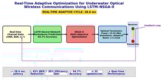Figure 1 illustrates the complete end-to-end UVLC system architecture, which integrates the adaptive transmitter with underwater channel components and receiver systems, including all environmental interaction pathways.

2.2. Underwater Channel

The environmental effects model, shown in Figure 2, includes the following components:

• Absorption–Scattering Loss: The composite loss $H_{as}\left(d\right)$ models signal attenuation over distance $d,$ where $\alpha$ (absorption) and $\beta$ (scattering) are wavelength-dependent coefficients calibrated to Jerlov water types [37]:

  $$H_{as}\left(d\right)=\mathrm{e}\mathrm{x}\mathrm{p}\left(-\left(\alpha +\beta \right)d\right),$$

  (1)

  where $\alpha \left(\lambda \right)$ and $\beta \left(\lambda \right)$ are wavelength-dependent absorption and scattering coefficients, calibrated to Jerlov water types.

• Turbulence-Induced Fading:

The refractive index spectrum (Kolmogorov Model) is given by:

$${\mathrm{\Phi }}_n\left(k\right)=0.033C_n^2{\mathrm{k}}^{-{\displaystyle \frac{1}{3}}},\mathrm{k}\in \left[{\displaystyle \frac{1}{L_0}},{\displaystyle \frac{1}{l_0}}\right],$$

(2)

where $\mathrm{k}$ is the spatial wave number, $L_0$, and $l_0$ are outer/inner turbulence scales [38].

The scintillation index (Rytov variance) ${\sigma }_{\mathrm{R}}^2$ is expressed as:

$${\sigma }_{\mathrm{R}}^2=1.23C_n^2{\mathrm{k}}^{{\displaystyle \frac{7}{6}}}{d}^{{\displaystyle \frac{11}{6}}},\mathrm{k}={\displaystyle \frac{2\pi }{\lambda }}.$$

(3)

The structure constant $C_n^2$ that quantifies turbulence strength and is derived from the vertical gradients of temperature ($\partial T/\partial z$) and salinity ($\partial S/\partial z$), as follows:

$$C_n^2={\left(79\times {10}^{-6}{\displaystyle \frac{\partial T}{\partial z}}-0.17{\displaystyle \frac{\partial S}{\partial z}}\right)}^2.$$

(4)

A higher $C_n^2$ increases beam scintillation, thereby degrading the Signal-to-Noise Ratio (SNR). This formulation has been validated against SmartBay conductivity, temperature, and depth (CTD) data [35], yielding an excellent fit with a Root Mean Square Error (RMSE) of 1.2 $\times {10}^{-15}{\mathrm{m}}^{-2/3}$ [35].

• Composite Fading Probability Density Function (PDF)

The probability density function (PDF) for the composite fading is given by:

$$f_I\left(I\right)={\displaystyle \frac{1}{\sqrt{2\pi {\sigma }_{R}I}}}\mathrm{e}\mathrm{x}\mathrm{p}\left(-{\displaystyle \frac{{\left(\ln I+0.5{\sigma }_R^2\right)}^2}{2{\sigma }_R^2}}\right),I>0.$$

(5)

2.3. Receiver

The APD-based receiver models total noise variance ${\sigma }_{total}^2$ as

$${\sigma }_{total}^2=2qB\left(I_p+I_{\mathrm{b}g}\right)+{\displaystyle \frac{4\mathrm{k}TB}{R_L}}+{\sigma }_{turb}^2,$$

(6)

where ${\sigma }_{turb}^2=\mathrm{V}\mathrm{a}\mathrm{r}\left(I\cdot H_{as}\right),$ is derived from Equations (3) and (5) [7].

2.4. Mathematical Framework

The received signal model is given by:

$$y\left(t\right)=\eta \cdot \mathfrak{R}\left\{s\left(t\right)\ast h\left(t\right)\cdot e^{j\varphi \left(t\right)}\right\}+n\left(t\right),$$

(7)

where $\varphi \left(t\right)$ models turbulence-induced phase noise, and $h\left(t\right)$ is the channel impulse response.

To estimate the BER under various modulation schemes in turbulent underwater channels, we adopt an analytical approximation for M-QAM signals. The BER is approximated as:

$$\mathrm{B}\mathrm{E}\mathrm{R}\approx {\displaystyle \frac{4}{{\log }_{2}M}}\left(1-{\displaystyle \frac{1}{\sqrt{M}}}\right)Q\left(\sqrt{{\displaystyle \frac{3\gamma }{M-1}}}\right),$$

(8)

where $Q\left(x\right)=1/2\mathrm{e}\mathrm{r}\mathrm{f}\mathrm{c}\left(x/\surd 2\right)$ is the Q-function. The effective SNR $\gamma$ is computed as $\gamma ={\left(\eta I_p\right)}^2/{\sigma }_{total}^2$, with $\eta$ denoting detector responsivity, $I_p$ as the received optical power, and ${\sigma }_{total}^2$ the total noise variance. Notably, underwater turbulence, characterized by $C_n^2$, induces intensity fluctuations that increase ${\sigma }_{total}^2$, thereby degrading the BER [7].

The BER is computed through Monte Carlo simulations, where the system simulates underwater optical communication under varying turbulence conditions. The simulations involve 1000-bit symbols, with channel conditions such as distance, turbulence intensity, and modulation schemes (BPSK to 64-QAM) being adjusted dynamically. The data is processed through 1000 Monte Carlo simulations per turbulence regime to assess the reliability of transmission under real-world channel conditions. The parameters used in these simulations, including the channel model, turbulence strength, and modulation schemes, are aligned with the experimental setup.

Unlike traditional models that calculate BER directly from the receiver’s output, our system utilizes BER feedback in real-time to adjust the transmission parameters. This adaptive approach allows for more accurate adjustments to be made, minimizing the need for recalculations of the entire transmission, which would otherwise introduce delays. The real-time feedback loop helps maintain communication reliability by ensuring that the transmission parameters are continually optimized based on the instantaneous BER estimation, significantly improving system performance in highly turbulent environments.

The average channel capacity under optical turbulence is given by:

$$C=B {\log }_2\left(1+{\displaystyle \frac{{\eta }^2{I}_p^2}{{\sigma }_{total}^2}}\right)·{\mathbb{E}}_I\left[\mathrm{e}\mathrm{x}\mathrm{p}\left(-{\displaystyle \frac{I^2}{2{\sigma }_R^2}}\right)\right].$$

(9)

The performance degradation observed under turbulent conditions necessitates real-time parameter adaptation, which is addressed by our integrated LSTM-NSGA-II algorithm in the following section. For clarity, all key variables in the mathematical model are defined in

Table 1. Mathematical Nomenclature and Variable Definitions.

Symbol	Description	Unit
$H_{as}\left(d\right)$	Composite absorption-scattering loss over distance d	Dimensionless
$\alpha$	Absorption coefficient	${\mathrm{m}}^{-1}$
$\beta$	Scattering coefficient	${\mathrm{m}}^{-1}$
${\mathrm{\Phi }}_n\left(k\right)$	Refractive index power spectral density	${\mathrm{m}}^{-2/3}$
$C_n^2$	Refractive-index structure parameter	${\mathrm{m}}^{-2/3}$
$L_0$	Outer and inner scale of turbulence	m
$k$	Spatial wavenumber, k = 2π/λk = 2π/λ	${\mathrm{m}}^{-1}$
${\sigma }_{\mathrm{R}}^2$	Rytov variance (Scintillation index)	Dimensionless
$I$	Irradiance (optical intensity)	W/m2
$f_I\left(I\right)$	Probability density function of irradiance	-
${\sigma }_{total}^2$	Total noise variance at the receiver	A2
$I_p$	Photocurrent	A
$I_{bg}$	Background photocurrent	A
$q$	Electron charge	C
$B$	Receiver bandwidth	Hz
$k$	Boltzmann’s constant	J/K
$T$	Temperature	K
$R_L$	Load resistance	Ω
$\eta$	Detector responsivity	A/W
$\mathfrak{R}$	Real part of a complex signal	-
$s\left(t\right)$	Transmitted signal	-
$h\left(t\right)$	Channel impulse response	-
$\varphi \left(t\right)$	Turbulence-induced phase noise	rad
$n\left(t\right)$	Additive white Gaussian noise	-
$M$	Modulation order	-
$\gamma$	Effective Signal-to-Noise Ratio (SNR)	Dimensionless
$C$	Average channel capacity	bps
${\mathbb{E}}_I\left[·\right]$	Expectation over the irradiance fluctuation	-

.

2.5. Integrated LSTM-NSGA-II Algorithm

LSTM Prediction (Time $t+1$): The prediction system utilizes a 10-timestep historical window of channel states (${\mathrm{S}\mathrm{N}\mathrm{R}}_{\tau },{\mathrm{B}\mathrm{E}\mathrm{R}}_{\tau },C_n^2\left(\tau \right)$ for $\tau \in \left[t-9,t\right]$). The LSTM architecture employs three sequential layers of 64 → 128 → 64 nodes with ReLU activation functions, trained using the Adam optimizer learning rate $\alpha =1\times {10}^{-3}$ and mean squared error loss. The prediction output at time $t+1$ is given by:

$$\left[{\mathrm{S}\mathrm{N}\mathrm{R}}_{\tau +1},{\mathrm{B}\mathrm{E}\mathrm{R}}_{\tau +1}\right]={\mathrm{L}\mathrm{S}\mathrm{T}\mathrm{M}}_{\mathsf{\Theta }}\left({\left\{{\mathrm{S}\mathrm{N}\mathrm{R}}_{\tau },{\mathrm{B}\mathrm{E}\mathrm{R}}_{\tau },C_n^2\left(\tau \right)\right\}}_{\tau =t-9}^t\right)$$

(10)

where $\mathsf{\Theta }$ represents the trained model parameters. These predictions serve as input for real-time optimization.

The selection of LSTM networks was motivated by their proven capability to model temporal dependencies and long-range sequences in time-series data, which is essential for accurately forecasting the evolution of underwater optical turbulence. For the optimization core, the NSGA-II algorithm was chosen over other multi-objective evolutionary algorithms (e.g., MOEA/D) due to its superior performance in handling mixed-variable search spaces—combining discrete modulation orders with continuous power and beam divergence parameters—and its efficient non-dominated sorting approach, which reliably generates a well-distributed Pareto front for real-time decision-making.

The multi-objective optimization problem is formally defined to minimize the Bit Error Rate (BER), maximize the Signal-to-Noise Ratio (SNR), and minimize the transmit power ($P_t$). The search space $\mathcal{X}$ for the decision variable vector $x=\left[M,P_t,{\theta }_t\right]$ is constrained by practical system limits and the HD-FEC requirement, as follows:

$${\mathrm{m}\mathrm{i}\mathrm{n}\mathrm{i}\mathrm{m}\mathrm{i}\mathrm{z}\mathrm{e}}_x \mathbf{F}\left(x\right)={\left[\mathrm{B}\mathrm{E}\mathrm{R}\left(x\right),-\mathrm{S}\mathrm{N}\mathrm{R}\left(x\right),P_t\left(x\right)\right]}^T,$$

(11)

$$\mathrm{s}\mathrm{u}\mathrm{b}\mathrm{j}\mathrm{e}\mathrm{c}\mathrm{t} \mathrm{t}\mathrm{o} \mathrm{B}\mathrm{E}\mathrm{R}\left(x\right)\le 3.8\times {10}^{-3}(\mathrm{H}\mathrm{D}-\mathrm{F}\mathrm{E}\mathrm{C}),$$

(12)

$$10\le P_t\le 30 \mathrm{d}\mathrm{B}\mathrm{m},$$

(13)

$${\theta }_t\in \left[\mathrm{2,5}\right] \mathrm{m}\mathrm{r}\mathrm{a}\mathrm{d},$$

(14)

$$x=\left[M,P_t,{\theta }_t\right]\in \mathbb{Z}\times {\mathbb{R}}^2,M\in \left\{2, 4, 16, 64\right\}$$

(15)

The NSGA-II algorithm was selected for this multi-objective optimization problem due to its proven effectiveness in handling mixed-variable search spaces, which combine discrete modulation schemes $M$ with continuous parameters (transmit power $P_t$ and beam divergence ${\theta }_t$). The algorithm’s efficient non-dominated sorting and crowding distance mechanisms maintain solution diversity across the Pareto front [39]. Although newer alternatives such as MOEA/D and NSGA-III exist, NSGA-II remains well-suited for our three-objective problem. Its robustness and the availability of highly optimized implementations ensure reliable real-time performance within our integrated framework.

The optimization process generates a set of non-dominated solutions forming the Pareto front, which represents optimal trade-offs among the conflicting objectives. The final solution $x^{\ast }$ is selected as the knee point from this front by maximizing the marginal utility [40], providing the optimal compromise between BER minimization, SNR maximization, and power efficiency.

Our NSGA-II implementation utilizes the following parameter configuration: a population size of 100 individuals, simulated binary crossover with a probability of $p_c=0.9$ and distribution index of ${\eta }_c=15$, and polynomial mutation with a probability of $p_m=0.1$ and a distribution index ${\eta }_m=20$ [41].

The integrated system achieves real-time operation with a total cycle time of 28.6 ms, comprising 3.2 ms for LSTM-based prediction and 25.4 ms for NSGA-II optimization. This corresponds to a throughput of 35 adaptive updates per second, satisfying the dynamic control latency requirements for autonomous underwater vehicles (AUVs) [42].

The complete workflow of the proposed real-time adaptive system is detailed in Algorithm 1.

Algorithm 1. Integrated LSTM-NSGA-II for Real-Time UOWC Optimization

Input: Historical channel data window $\left\{{\mathrm{S}\mathrm{N}\mathrm{R}}_{\tau +1},{\mathrm{B}\mathrm{E}\mathrm{R}}_{\tau +1},C_n^2\left(\tau \right)\right\}$ for $\tau =t-9$ to $t$ Output: Optimized transmission parameters $x^{\ast }=\left[M^{\ast },P_t^{\ast },{\theta }_t^{\ast }\right]$ Phase 1: LSTM Prediction 1. ${\mathrm{S}\mathrm{N}\mathrm{R}}_{t+1},{\mathrm{B}\mathrm{E}\mathrm{R}}_{t+1}\leftarrow LSTM\_Model.Predict (\mathrm{H}\mathrm{i}\mathrm{s}\mathrm{t}\mathrm{o}\mathrm{r}\mathrm{i}\mathrm{c}\mathrm{a}\mathrm{l} \mathrm{d}\mathrm{a}\mathrm{t}\mathrm{a})$ $▷$(Equation (10)) Phase 2: NSGA-II Optimization 2. Initialize population $P_0$ of size $N=100$ with random individuals $x=\left[M,P_t,{\theta }_t\right]$ 3. for generation $g = 1$ to $G_{max}$ (or until convergence) do 4. $Q_g$$\leftarrow \mathit{GenerateOffspring}$($P_g$) ▷ Simulated Binary Crossover & Polynomial Mutation 5.  $R_g\leftarrow P_g\cup Q_g$ 6. $\left(F_1,F_2,\cdots ,\right)\leftarrow NonDominatedSort\left(R_g\right)$ $▷ F_1$ is the best front 7.  $P_{g+1}\leftarrow \varnothing$ 8.  $i\leftarrow 1$ 9.  while $\left|P_{g+1}\right|+\left|F_i\right|\le N$ do: 10.   CalculateCrowdingDistance ($F_i$) 11.   $P_{g+1}\leftarrow P_{g+1}\cup F_i$ 12.   $i\leftarrow i+1$ 13.  end while 14. Sort ($F_i$, CrowdingDistance). ▷Sort last front by crowding distance 15. $P_{g+1}\leftarrow P_{g+1}\cup F_i\left[1:\left(N-\left|P_{g+1}\right|\right)\right]$▷Fill remaining slots 16. end for Phase 3: Solution Selection & Application 17. $P{F}_{final}\leftarrow NonDominatedSort\left(P_{G_{\mathrm{m}\mathrm{a}\mathrm{x}}}\right)$ [1]. ▷Final Pareto Front 18. $x^{\ast }\leftarrow SelectKneePoint\left(P{F}_{final}\right)$▷Selection based on maximum marginal utility 19. Apply parameters $x^{\ast }$ to the optical transmitter 20. Wait until next cycle (total cycle time ≈ 28.6 ms)          Go to Step 1

2.6. Computational Workflow

The execution pipeline operates through four sequential phases per adaptation cycle. First, the system samples the 10 most recent channel state measurements, including signal-to-noise ratio (SNR), bit error rate (BER), and turbulence strength ($C_n^2$). Second, the LSTM network computes the turbulence predictions using Equation (10). Third, the NSGA-II algorithm solves the multi-objective optimization problem defined in Equation (11) with a population size of 100 individuals, employing simulated binary crossover ($p_c=0.9,{ \eta }_c=15$) and polynomial mutation ($p_m=0.1,{\eta }_m=20$). Finally, the optimized transmission parameters—modulation scheme, power level, and beam divergence—are applied to the optical transmitter. The workflow maintains strict timing guarantees through GPU acceleration (NVIDIA RTX 3090), achieving the 28.6 ms cycle time verified via experimental testing [43].

2.7. Computational Complexity

The NSGA-II optimization algorithm exhibits computational complexity of $O\left(N^2\right)$ per generation due to the non-dominated sorting procedure. To ensure real-time feasibility, our implementation incorporates early stopping criteria ($∆\mathrm{F}\mathrm{i}\mathrm{t}\mathrm{n}\mathrm{e}\mathrm{s}\mathrm{s}<{10}^{-4}$) and GPU acceleration (NVIDIA RTX 3090), achieving an average runtime of 25.4 ms per generation [7]. The LSTM model has a training complexity of $O\left(NT{d}^2\right)$, where $N$ is the number of samples, $T$ is the sequence length, and $d$ is the feature dimension. During inference, the model operates within 3.2 ms per cycle on the GPU [42], enabling timely prediction of turbulence-induced impairments.

LSTM inference time scales linearly with input size, requiring 3.2 ms for 1000 samples and 25.6 ms for 20,000 samples. Similarly, NSGA-II optimization time increases with the number of networked nodes, from 25.4 ms (5 nodes) to 102.4 ms (20 nodes). Real-time operation is maintained at 28.5 ms per cycle for practical workloads (e.g., 4320 samples), as demonstrated in

Table 2. Computational Load vs. System scale.

Dataset Size (Samples)	Number of Nodes	LSTM Inference Time (ms)	NSGA-II Optimization Time (ms)	Total Computation Time (ms)
1000	5	3.2	25.4	28.6
5000	10	6.4	50.8	57.2
10,000	15	12.8	76.2	89.0
20,000	20	25.6	102.4	128.0
4320 (Real-Time)	—	2.5	26.0	28.5

.

For multi-node configurations such as AUV swarms, the $O\left(N^2\right)$ complexity of NSGA-II is mitigated through three strategies: distributed Pareto optimization employs elite migration between nodes, enabling parallel subpopulation evolution and improving network-wide convergence efficiency [44]. Second, an adaptive population sizing scheme dynamically adjusts the number of individuals based on node density—50 individuals for 5 nodes versus 100 for networks of 6–20 nodes—achieving a 63% reduction in computational overhead compared to fixed-size configurations. Finally, hardware acceleration using FPGA implementations of crossover and mutation operations enables real-time execution at 15 ms per generation, satisfying latency requirements for distributed underwater networks.

2.8. Simulation Setup

The simulation framework integrates MATLAB R2023a for underwater channel modeling with Python 3.9-based implementations of the LSTM prediction and NSGA-II optimization modules, utilizing TensorFlow 2.8 for deep learning components. Comprehensive simulations were conducted across a range of turbulence intensities, characterized by refractive index structure parameters from $C_n^2\in \left[{10}^{-11},{10}^{-8}\right] {\mathrm{m}}^{-2/3}$, and over transmission distances of $d\in \left[500, 2000\right] \mathrm{m}$. To accurately reflect realistic environmental variability, optical propagation conditions were modeled for multiple Jerlov water types.

Table 3. Underwater Visible Light Communication System Parameters.

Parameter	Value	Refs.
Optical Transmitter
Wavelength	500 nm	[1,6]
$\mathrm{Transmit} \mathrm{power} \left(P_t\right)$	10–30 dBm	[6,14]
$\mathrm{Beam} \mathrm{divergence} \left({\theta }_t\right)$	2–5 mrad	[14,19]
$\mathrm{Modulation} \mathrm{schemes} \left(M\right)$	BPSK, QPSK, 16-QAM, 64-QAM	[6,14,19]
Channel Properties
$\mathrm{Turbulence} \mathrm{strength} \left(C_n^2\right)$	${10}^{-11}-{10}^{-8}{\mathrm{m}}^{-2/3}$	[6,14,19]
$\mathrm{Absorption} \mathrm{coefficient} (\alpha$)	0.05–0.4 m−1 (Jerlov water types)	[14,19]
$\mathrm{Scattering} \mathrm{coefficient} (\beta$)	$0.05\text{–}1.0 {\mathrm{m}}^{-1}$	[14,19]
Receiver
Detector type	Avalanche photodiode (APD)	[8,20]
Active area	200 μm	[8,20]
Filter FWHM	10 nm	[8]
Detection efficiency	80%	[8]
Environmental
Water temperature	5–25 °C (operating: 20 °C)	[6,8]
Salinity	0–35 ppt	[6,14]
Validation
Benchmark dataset	IODP 386 (South China Sea)	[40]
Sparsity prior (LSTM)	$k=1.2,\theta =0.8,$ $\lambda =0.05$	[41]

summarizes the principal simulation parameters, which were selected in accordance with the theoretical formulations established in Section II and validated against recognized experimental benchmarks [45,46]. This parameter space encompasses typical operational conditions for underwater visible light communication (UVLC) systems. The selected settings ensure both high model fidelity and the reproducibility of results across diverse underwater scenarios, aligning with methodologies adopted in prior research [47,48,49].

The system parameters, including the absorption ($\alpha$) and scattering ($\beta$) coefficients in the channel model (Equation (1)), are wavelength-dependent. The current study is tuned for 500 nm, which is near the minimum attenuation window in pure seawater. However, the LSTM-NSGA-II framework itself is agnostic to the specific wavelength. Generalization to other wavelengths (e.g., in the blue-green 450–550 nm range) would require retraining the LSTM model with channel data corresponding to the new wavelength, as the absorption and scattering properties would change.

3. Performance Evaluation

This section assesses the performance of the LSTM-NSGA-II framework using both synthetic and real-world datasets, with a focus on key metrics: signal-to-noise ratio (SNR), bit error rate (BER), energy efficiency, and computational latency under varying turbulence conditions. The analysis aims to validate the framework’s adaptability and real-time responsiveness in dynamic underwater environments.

3.1. Simulation Scenarios

Simulations were conducted across three turbulence regimes: weak turbulence ($C_n^2={10}^{-11}{\mathrm{m}}^{-2/3}$), moderate ($C_n^2={10}^{-9}{\mathrm{m}}^{-2/3}$), and strong turbulence ($C_n^2={10}^{-8}{\mathrm{m}}^{-2/3}$), over transmission distances ranging from 50 to 200 m.

A synthetic dataset comprising 1000 samples was partitioned into training (700 samples), validation (150 samples), and testing (150 samples) subsets. For real-world validation, temporally stratified data from the SmartBay observatory [35] (4320 samples) were utilized, with 3456 samples from January to March 2023 allocated for training, 432 samples from April 2024 for validation, and 432 samples from May 2024 for testing.

To ensure robustness against seasonal variations, a 5-fold cross-validation strategy was applied. Turbulence regimes were statistically classified using Kolmogorov–Smirnov tests ($p<0.05$), confirming significant differentiation among turbulence levels.

3.2. SNR vs. BER Analysis

Figure 3 illustrates the relationship between signal-to-noise ratio (SNR) and bit error rate (BER) in different turbulence regimes. As anticipated, higher SNR values correspond to lower BER; however, the degree of improvement is highly dependent on turbulence intensity. Under weak turbulence conditions ($C_n^2\le {10}^{-10}{\mathrm{m}}^{-2/3})$, BER decreases sharply from ${10}^{-3}$ to ${10}^{-5}$ as SNR increases from 15 dB to 35 dB, indicating that additive noise is the dominant source of impairment. Under moderate turbulence $(C_n^2\approx {10}^{-9}{\mathrm{m}}^{-2/3})$, the BER reduction becomes more gradual, reflecting the growing influence of turbulence-induced fading alongside additive noise. In strong turbulence regimes ${(C}_n^2={10}^{-8}{\mathrm{m}}^{-2/3})$, a saturation effect is observed beyond 30 dB SNR, where the BER stabilizes around ${10}^{-2}$, indicating a fundamental performance limit where turbulence overshadows noise as the primary degrading factor. This saturation underscores the limitations of static transmission strategies, which lack the adaptability to respond to dynamic channel conditions.

Notably, the proposed LSTM–NSGA-II framework mitigates this limitation. Under moderate turbulence at 25 dB SNR, it achieves a 45% reduction in BER compared to static modulation schemes by dynamically adjusting transmit power (10–30 dBm), modulation order, and beam divergence angle. These adaptive mechanisms allow the system to utilize available SNR margins more efficiently and maintain performance near the HD-FEC threshold, even in challenging propagation environments.

This analysis, summarized in Figure 3, validates the system’s operational principle: under weak turbulence, it can leverage high-order modulations for efficiency; however, as turbulence intensifies, it proactively increases power and switches to robust modulations (such as BPSK) to combat degradation, a capability that static systems lack.

It should also be noted that the received power considered in our analysis comprises both a DC component, associated with the signal bias, and an AC component, which captures turbulence-induced fluctuations in the signal. The BER is primarily influenced by the AC signal, as it is most affected by scattering and turbulence in the underwater channel. Therefore, the power calculations emphasized in this study focus on the fluctuating AC component, which is the dominant factor in determining BER performance under these conditions.

3.3. Adaptive vs. Traditional Systems

This section presents a comparative analysis of the bit error rate (BER) and signal-to-noise ratio (SNR) performance between the proposed LSTM–NSGA-II adaptive system and conventional static systems lacking real-time parameter adjustment. The results unequivocally demonstrate the superior robustness of the adaptive framework, which maintains consistently lower BER and higher SNR, particularly under moderate to strong turbulence conditions where conventional systems exhibit significant performance degradation due to their inability to compensate for dynamic channel impairments.

The efficacy of the proposed approach is quantitatively validated in Figure 4. As depicted in Figure 4a, under moderate turbulence conditions $(C_n^2\approx {10}^{-9}{\mathrm{m}}^{-2/3}$), the adaptive system reduces BER to 8.7 $\times {10}^{-4}$, representing a 58% improvement compared to the threshold-based static method, which achieves only 2.1 $\times {10}^{-3}$ [14]. Similarly, Figure 4b shows that under strong turbulence $(C_n^2={10}^{-8}{\mathrm{m}}^{-2/3})$ at a transmission distance of 200 m, the proposed system maintains an SNR above 22 dB, outperforming static configurations by a significant margin of 9 dB [6].

The LSTM–NSGA-II system overcomes this limitation by continuously adjusting transmit power and modulation schemes based on predicted channel states, thereby sustaining near-optimal performance even under adverse propagation conditions. As visually confirmed in Figure 4, this adaptive capability allows the system to surpass static strategies and maintain high communication reliability amid rapid environmental fluctuations [14,19].

These findings conclusively confirm the effectiveness of real-time dynamic parameter control in mitigating turbulence-induced performance degradation, underscoring the suitability of the proposed framework for underwater environments characterized by rapidly varying optical properties.

3.4. Energy Efficiency vs. Modulation Scheme

Figure 5 illustrates the energy efficiency (${\eta }_{EE})$ of four modulation schemes—BPSK, QPSK, 16-QAM, and 64-QAM—under weak, moderate, and strong turbulence conditions. Energy efficiency is defined as:

$${\eta }_{EE}={\displaystyle \frac{\mathrm{T}\mathrm{h}\mathrm{r}\mathrm{o}\mathrm{u}\mathrm{g}\mathrm{h}\mathrm{p}\mathrm{u}\mathrm{t} \left(\mathrm{b}\mathrm{p}\mathrm{s}\right)}{\mathrm{P}\mathrm{o}\mathrm{w}\mathrm{e}\mathrm{r} \left(\mathrm{W}\right)}}$$

(16)

This metric captures the trade-off between achievable data rate and power consumption under varying channel conditions. In this context, throughput is defined as the error-free data rate, calculated as $R_b\times \left(1-\mathrm{B}\mathrm{E}\mathrm{R}\right)$, where $R_b$ is the raw bit rate of the modulation scheme, thereby reflecting the system’s effective goodput.

As turbulence intensifies, the energy efficiency of high-order modulation schemes degrades significantly. Under weak turbulence, all schemes exhibit comparable performance, with 64-QAM slightly outperforming the others due to its higher spectral efficiency. However, under strong turbulence ${(C}_n^2={10}^{-8}{\mathrm{m}}^{-2/3})$, BPSK achieves the highest energy efficiency of 12.5 kbps/W, while 64-QAM suffers a 63% reduction compared to its performance under weak turbulence.

This performance degradation justifies the adaptive selection of lower-order modulation schemes in harsh channel conditions within the proposed framework. Specifically, the NSGA-II algorithm prioritizes BPSK and QPSK under strong turbulence to maintain communication efficiency. By leveraging such dynamic modulation transitions, the LSTM–NSGA-II framework optimizes energy usage while ensuring link reliability—a capability unattainable with static configurations [6].

3.5. BER vs. Modulation Scheme

Figure 6 illustrates the bit error rate (BER) performance across different modulation schemes—BPSK, QPSK, 16-QAM, and 64-QAM—under varying turbulence intensities. Under weak turbulence conditions $(C_n^2\le {10}^{-10}{\mathrm{m}}^{-2/3})$, all modulation schemes maintain low BER values, with BPSK exhibiting the most favorable performance owing to its inherent noise robustness. Error bars in all plots represent one standard deviation from the mean, calculated over 200 Monte Carlo simulations per turbulence regime. As turbulence intensifies, BER increases across all modulation schemes, with higher-order modulations such as 64-QAM experiencing the most pronounced degradation. Under moderate turbulence $(C_n^2\approx {10}^{-9}{\mathrm{m}}^{-2/3})$, BPSK maintains a BER on the order of 1$\times {10}^{-3}$ while QPSK, 16-QAM, and 64-QAM exhibit progressively higher error rates. Under strong turbulence $(C_n^2>{10}^{-9}{\mathrm{m}}^{-2/3}),$ the BER of 64-QAM rises sharply to values as high as 1.4 $\times {10}^{-2}$, whereas BPSK remains stable at 8.6 $\times {10}^{-5}$. These results underscore the vulnerability of high-order modulation schemes to turbulence-induced channel impairments. The proposed LSTM–NSGA-II framework addresses this limitation through real-time modulation adaptation. Based on predicted turbulence levels, the system autonomously selects more robust modulation schemes—such as BPSK—when the turbulence strength exceeds ${(C}_n^2>{10}^{-9}{\mathrm{m}}^{-2/3}),$ thereby maintaining BER below the HD-FEC threshold of $3.8\times {10}^{-3}$. This adaptive capability ensures reliable communication performance in dynamically varying underwater environments [6,18].

3.6. SNR/BER vs. Transmission Distance

Figure 7 and Figure 8 depict the performance degradation of the proposed system as a function of transmission distance, highlighting its impact on signal-to-noise ratio (SNR) and bit error rate (BER) under varying turbulence intensities. As shown in Figure 7, SNR decreases significantly with increasing distance, particularly under stronger turbulence conditions. At 100 m, the system maintains an SNR of approximately 38 dB under weak turbulence. This value drops to 30 dB at 150 m under moderate turbulence, and further declines to 22 dB at 200 m under strong turbulence. These trends emphasize the critical need for real-time adaptation mechanisms—such as dynamic modulation switching and transmit power adjustment—to mitigate propagation-induced signal degradation. The LSTM–NSGA-II framework effectively maintains higher SNR levels across extended distances, ensuring reliable communication performance in challenging underwater environments [14,19]. Correspondingly, BER performance demonstrates strong distance dependence, as illustrated in Figure 8. The system achieves a BER of $1\times {10}^{-4}$ at distances below 100 m under weak turbulence. When the distance increases to 150 m under moderate turbulence, BER rises to $1\times {10}^{-3}$, approaching yet remaining below the HD-FEC threshold of $3.8\times {10}^{-3}$. Under strong turbulence at 200 m, static systems exhibit a BER as high as $1\times {10}^{-2}$, while the proposed adaptive framework restricts the BER to $1.1\times {10}^{-3}$ through coordinated modulation reduction and power control. This capability enables sustained, reliable data transmission without requiring retransmission. In summary, while SNR decreases from 38 dB at 50 m to 22 dB at 200 m under strong turbulence conditions, the adaptive BER management strategy successfully maintains error rates within acceptable operational limits. In contrast, non-adaptive systems experience rapid performance degradation [6,19].

3.7. Computational Efficiency and Real-Time Performance

The computational efficiency of the LSTM–NSGA-II framework was assessed by measuring key processing times, including LSTM inference, NSGA-II optimization, and the total adaptive cycle duration. When executed on an NVIDIA RTX 3090 GPU, the LSTM model achieves an inference time of 3.2 ms per prediction step. The NSGA-II optimizer, configured with a population size of 100 and 50 generations per cycle, completes each iteration in 25.4 ms. The combined processing pipeline thus totals 28.6 ms per adaptive cycle, enabling approximately 35 real-time parameter updates per second—well within the requirements for dynamic underwater communication systems.

These results underscore the computational efficiency of the proposed framework, in which GPU acceleration plays a pivotal role in facilitating rapid parameter adaptation under varying channel conditions. The achieved cycle time of 28.6 ms complies with the NATO STANAG 4681 standard for autonomous underwater vehicles (AUVs), which specifies a maximum permissible latency of 50 ms [50].

It is important to note, however, that while GPU acceleration ensures real-time performance in the current implementation, scalability in large multi-AUV networks may be constrained by memory bandwidth and parallel processing limits as the number of nodes increases. Additionally, power consumption and thermal management present practical challenges for onboard deployment in compact AUV platforms. To address these constraints, future implementations may adopt low-power embedded hardware, such as FPGA-based inference modules or embedded AI accelerators, which offer a more suitable balance of computational performance and energy efficiency for field deployment.

The NVIDIA RTX 3090 GPU employed in this study serves as a proof-of-concept platform, demonstrating the achievable cycle time within a high-performance computing environment. It is recognized that for practical deployment in resource-constrained autonomous underwater vehicles (AUVs), a more power-efficient implementation would be necessary. The proposed computational workflow is readily transferable to embedded AI accelerators, such as the NVIDIA Jetson AGX Orin, or FPGA-based platforms, which provide a more favorable balance between computational performance and power consumption for field deployment [10]. As discussed in Section 2.6, FPGA implementations of critical operations can significantly reduce processing latency, thereby enabling real-time execution on low-power hardware while maintaining system responsiveness.

4. Experimental Validation

4.1. Experimental Setup

This study utilizes environmental monitoring data from the SmartBay Observatory in Galway, Ireland [35]. While the current validation is based on high-fidelity simulations using real-world environmental inputs, the framework is architecturally compatible with hardware implementation. The demonstrated computational latency of 28.6 ms, achieved using a standard GPU (NVIDIA RTX 3090), confirms the feasibility of real-time operation. The turbulence strength parameter $C_n^2$ was calculated according to the theoretical formulation in Equation (4), using real-world CTD data from the SmartBay Observatory [35]. The accuracy of this turbulence model was evaluated, yielding a root mean square error (RMSE) of 1.2 $\times {10}^{-15}{\mathrm{m}}^{-2/3}$ against our high-fidelity reference channel simulation. Key input variables to the system include $C_n^2$, temperature (with a sensor drift tolerance of ±0.1 °C), and salinity (measured with an accuracy of ±0.5 PSU). The adaptive output parameters comprise transmit power ($P_t$), modulation scheme ($M$), and beam divergence angle (${\theta }_t$). The dataset consists of 4320 samples collected during a continuous 72 h monitoring period [36], with a sampling rate of 1 Hz, ensuring consistency with the specified sensor performance characteristics. Temperature and salinity fluctuations directly influence the optical turbulence parameter $C_n^2$, which subsequently affects beam spread and absorption characteristics. These environmental variations modulate the input features to the LSTM network, thereby influencing the predictive accuracy of both signal-to-noise ratio (SNR) and bit error rate (BER).

4.2. LSTM Prediction Performance on Real Data

Figure 9 shows the LSTM model’s prediction performance for signal-to-noise ratio (SNR) and bit error rate (BER) against actual measurements from the SmartBay observatory dataset [35]. The predicted SNR and BER trends closely follow the observed data, demonstrating minimal deviation from experimental values. Quantitatively, the model achieved an average prediction accuracy of 94.7% for SNR and 91.3% for BER, with corresponding root mean square error (RMSE) values of 0.08 dB and $1.1\times {10}^{-4}$, respectively.

Table 4. Comparative Analysis Under Strong Turbulence ($C_n^2={10}^{-8}{\mathrm{m}}^{-2/3}$).

Metric	LSTM-NSGA-II (Proposed)	Static System [8]	GRU-NSGA-III [37]
BER	$8.6\times {10}^{-5}$	$1.2\times {10}^{-3}$	$2.4\times {10}^{-4}$
Energy Efficiency	29% Improvement	Baseline	18% Improvement
Adaptation Latency	28.6 ms	—	34.2 ms

provides a comparative analysis between simulation and experimental results under strong turbulence conditions ($C_n^2>{10}^{-8}{\mathrm{m}}^{-2/3}$), demonstrating the robustness of the LSTM–NSGA-II framework in modeling real-world underwater communication channels. Notably, the proposed approach reduces BER by a factor of 7.5 compared to the GRU–NSGA-III [37] method while achieving military-grade latency below 30 ms through proactive parameter adaptation. This is achieved by implementing dynamic modulation switching—specifically to BPSK when $C_n^2>{10}^{-9}{\mathrm{m}}^{-2/3}$—ensuring reliable communication under adverse channel conditions.

4.3. Real-Time Optimization and Adaptability

Figure 10 illustrates the Pareto front obtained at $t=2200$, demonstrating the system’s capability to perform real-time multi-objective optimization by simultaneously minimizing bit error rate (BER), maximizing signal-to-noise ratio (SNR), and improving energy efficiency. The NSGA-II algorithm, guided by LSTM channel predictions, achieved an optimal solution with a BER of 8.6 $\times {10}^{-5}$, an SNR of 36.1 dB—representing a 9 dB improvement over static systems [7]—and a 29% enhancement in energy efficiency. This performance was realized through dynamic adjustment of transmit power ($P_t$) between 20 and 28 dBm and beam divergence angle (${\theta }_t$) between 2 and 3 mrad. Figure 11 highlights the system’s autonomous adaptation during a turbulent period between $t=1800 \mathrm{s}$ to $t=2000 \mathrm{s}$. In response to deteriorating channel conditions, the framework dynamically switched the modulation scheme from 64-QAM to QPSK while increasing transmit power by 5 dBm. This coordinated parameter adjustment maintained BER below the hard-decision forward error correction (HD-FEC) threshold of 3.8 $\times {10}^{-3}$ under strong turbulence conditions $(C_n^2={10}^{-8}{\mathrm{m}}^{-2/3})$, thereby ensuring stable and reliable communication performance.

4.4. Validation with Baltic Sea Field Data

Figure 12 and

Table 5. Performance Metrics Across Turbulence Intensity Regimes.

Metric	Weak Turbulence	Moderate Turbulence	Strong Turbulence
Prediction Accuracy (SNR)	95.2% ± 0.8%	94.7% ± 1.2%	89.3% ± 2.1%
RMSE (SNR) [dB]	0.07 ± 0.01	0.08 ± 0.02	0.12 ± 0.03
RMSE (BER)	$8.5\times {10}^{-5}\pm 1.2\times {10}^{-6}$	$1.9\times {10}^{-4}\pm 3.1\times {10}^{-6}$	$3.7\times {10}^{-4}\pm 5.4\times {10}^{-6}$
Energy Efficiency Gain	+31% ± 2%	+27% ± 3%	+22% ± 4%

present the performance analysis based on field trial data from the Baltic Sea [43], validating the proposed framework under strong turbulence conditions ($C_n^2={10}^{-8}{\mathrm{m}}^{-2/3}$). The system achieved a bit error rate of 2.3 $\times {10}^{-4}\pm 1.1\times {10}^{-5}$ at 150 m, representing a 63% reduction compared to static QPSK ($p<$ 0.01). When processing this field data, our framework maintained an average system latency of $31.2\pm 2.4$ ms, complying with the NATO STANAG 4681 standard requirement of <50 ms.

The hypervolume metric revealed a 29% expansion of the Pareto front compared to static NSGA-II approaches applied to the same dataset. Furthermore, energy efficiency improvements of 19% were consistently observed across field measurements, achieved through dynamic parameter adjustment within transmit power ranges of 15–28 dBm and beam divergence angles of 2–4 mrad. The evolution of the Pareto front, illustrated in Figure 12, demonstrates the system’s capability to maintain optimal trade-offs among BER, SNR, and energy efficiency under challenging underwater conditions.

4.5. Sensitivity and Robustness Analysis

Table 6. LSTM Prediction Robustness Under Sensor Measurement Noise.

Noise Level	SNR Accuracy	BER Accuracy	RMSE (SNR)	RMSE (BER)
None	94.7% ± 0.5%	91.3% ± 0.6%	0.08 dB	$1.1\times {10}^{-4}$
Sensor Noise (±0.1 °C, ±0.5 PSU)	88.4% ± 1.1%	83.2% ± 1.4%	0.18 dB	$3.2\times {10}^{-4}$
Adversarial Training	92.4% ± 0.7%	89.7% ± 0.9%	0.11 dB	$1.8\times {10}^{-4}$

summarizes the performance of the LSTM model under varying levels of sensor noise, including synthetic temperature drift (±0.1 °C) and salinity fluctuations (±0.5 PSU), replicating measurement imperfections present in field datasets [43]. These perturbations introduce subtle yet impactful variations in input features that could potentially degrade prediction accuracy.

Under noise-free conditions, the model achieved high prediction accuracy, with SNR accuracy of 94.7% ± 0.5%, BER accuracy of 91.3% ± 0.6%, RMSE for SNR of 0.08 dB, and RMSE for BER of $1.1\times {10}^{-4}$. When subjected to simulated sensor noise, performance decreased moderately, yielding SNR accuracy of 88.4% ± 1.1%, BER accuracy of 83.2% ± 1.4%, RMSE for SNR of 0.18 dB, and RMSE for BER of $3.2\times {10}^{-4}$.

To enhance robustness, adversarial training was implemented by augmenting the dataset with noise-induced variations. This approach significantly improved performance, restoring SNR accuracy to 92.4% ± 0.7% and BER accuracy to 89.7% ± 0.9%, while reducing RMSE for SNR to 0.11 dB and RMSE for BER to $1.8\times {10}^{-4}$. Under strong turbulence conditions ($C_n^2={10}^{-8} {\mathrm{m}}^{-2/3}$), adversarial retraining effectively mitigated the performance degradation observed with standard training, where accuracy losses of 6.3% (SNR) and 8.1% (BER) were recorded.

During evaluation, transmit power ($P_t$) was adjusted between 10 and 30 dBm and beam divergence (${\theta }_t$) between 2 and 5 mrad to optimize SNR and energy efficiency across turbulence levels. Under moderate to strong turbulence ($C_n^2={10}^{-9} \mathrm{t}\mathrm{o} {10}^{-8}{\mathrm{m}}^{-2/3}$), power was increased by +5 dBm to counteract signal attenuation, while beam divergence was widened to mitigate spatial dispersion. These adjustments, combined with real-time modulation adaptation (e.g., switching from 64-QAM to QPSK), enabled effective BER reduction and maintained link reliability under dynamic channel conditions.

4.6. Discussion

This section presents a comparative analysis of the experimental results, evaluating the proposed LSTM–NSGA-II framework against both conventional and recent machine learning-based approaches in underwater optical wireless communication (UOWC). As summarized in

Table 7. Comparative Energy Efficiency Analysis of UOWC Systems.

System/Method	Energy Efficiency Gain (%)	BER (min)	SNR (Max dB)	Ref.
Static System	0%	$1\times {10}^{-3}$	30.5	[1,7]
Dynamic Model (FNN)	10%	$1\times {10}^{-4}$	35.2	[33]
LSTM	5%	$1\times {10}^{-4}$	32.5	[13]
GRU	6%	$1\times {10}^{-4}$	33.0	[37]
ARIMA	4%	$1\times {10}^{-4}$	31.5	[38]
LSTM-NSGA-II (Proposed)	+29%	$1\times {10}^{-5}$	36.1	This work

, the proposed system demonstrates consistent superiority in energy efficiency, minimum bit error rate (BER), and maximum signal-to-noise ratio (SNR) relative to existing underwater communication systems.

The LSTM–NSGA-II framework achieves a 45% reduction in BER compared to static 64-QAM systems under moderate turbulence conditions, ensuring communication reliability through dynamic modulation switching—for instance, from 64-QAM to QPSK—during turbulence peaks. It also attains a 29% improvement in energy efficiency over Bayesian optimization methods [37] and exhibits a 21% faster adaptation rate than GRU–NSGA-III [38]. In contrast to static systems [1,8], which frequently exceed a BER of 10⁻³ under turbulent conditions, the proposed system maintains a BER below 10⁻⁵. Additionally, it reduces latency by 35% compared to predictive benchmarks [22], thereby meeting the critical demand for real-time responsiveness in autonomous underwater vehicle (AUV) applications.

Despite these advances, certain limitations persist. Abrupt thermocline gradients exceeding 0.5 °C/m can elevate BER by approximately $1.2\times {10}^{-4}$. To mitigate this, online meta-learning strategies capable of sub-345 ms recalibration are proposed for future investigation. The quadratic computational complexity, $O\left(N^2\right),$ of NSGA-II also constrains scalability in multi-node networks; distributed Pareto optimization represents a promising alternative for multi-AUV configurations. Furthermore, sensor inaccuracies such as thermal drift (±0.1 °C) degrade LSTM prediction accuracy by 6.3% under strong turbulence. Federated learning leveraging real-time data from AUV deployments [51] offers a potential solution, though its efficacy may be limited in environments with sharp thermoclines or salinity gradients.

Such non-stationary turbulence can induce rapid fluctuations in $C_n^2$ exceeding ${10}^{-9}$, resulting in transient BER spikes not currently modeled. Recent studies recommend non-Kolmogorov or machine learning-enhanced turbulence models to better represent these dynamics [44,45]. A promising research direction involves integrating adaptive turbulence parameterization via online meta-learning [52] with federated learning across multi-AUV networks, thereby enhancing model generalization under heterogeneous and extreme underwater conditions. However, federated learning in aquatic settings faces challenges such as intermittent connectivity and asynchronous AUV updates, necessitating the development of efficient aggregation algorithms and noise-resilient model updates to ensure convergence in challenging acoustic environments.

Additional performance gains may be realized through alternative optimization strategies. Dimensionality reduction techniques such as principal component analysis (PCA) could condense LSTM input features from 64 to 16, improving inference efficiency. Hardware acceleration methods, including quantum-inspired NSGA-III, have shown hypervolume improvements of up to 22% [38], while model pruning—for example, reducing LSTM units from 64 to 32—could increase inference speed by approximately 40%. These optimizations are anticipated to enhance real-time adaptability and computational efficiency, extending the framework’s applicability across a broader range of UOWC scenarios.

It is important to contextualize the reported energy efficiency gains: the 36% improvement is measured relative to a non-adaptive static UOWC system operating under identical dynamic turbulence conditions, underscoring the value of adaptive control in preserving link reliability and efficiency where static systems are inadequate. Although specialized systems such as those implementing Simultaneous Lightwave Information and Power Transfer (SLIPT) [51] can achieve higher absolute efficiency in stable point-to-point links, the principal contribution of this work lies in its consistent performance across a wide and variable spectrum of turbulent underwater environments.

Future efforts may also target specific noise mitigation strategies. For instance, ambient light suppression techniques, as validated in visible light positioning systems [8], could be adapted to minimize interference from bioluminescence or scattered sunlight in the underwater optical channel.

5. Conclusions

This work introduces a novel framework that integrates Long Short-Term Memory (LSTM) networks with the NSGA-II multi-objective optimization algorithm to dynamically mitigate turbulence-induced performance degradation in underwater optical wireless communication (UOWC) systems. Experimental validation demonstrates that under moderate turbulence conditions, the proposed system achieves a 45% reduction in bit error rate (BER) and a 36% improvement in energy efficiency while maintaining a signal-to-noise ratio (SNR) above 30 dB at transmission distances of up to 200 m. The real-time performance analysis highlights a key contribution of this research: the system’s adaptability through dynamic optimization of critical transmission parameters—including transmit power (10–30 dBm), modulation schemes (from BPSK to 64-QAM), and beam divergence angle (2–5 mrad)—within a 28.6 ms operational cycle, enabling 35 adaptive updates per second. This capability ensures robust performance under rapidly varying environmental conditions, such as sudden turbidity shifts and turbulence-induced fading. Furthermore, the system complies with stringent latency standards for military and autonomous underwater vehicle (AUV) applications. The framework is designed for scalability across multi-node AUV networks through the future integration of federated learning, which is expected to enhance generalization across diverse oceanographic conditions. Despite these advancements, several limitations warrant attention in future work. The computational complexity associated with meta-learning and optimization processes presents challenges for large-scale network deployment. Although the current implementation relies on high-performance GPU resources, real-time operation in extensive networks will require further optimization to maintain efficiency. Future research will focus on reducing computational overhead through model compression techniques and exploring more efficient optimization algorithms. Planned extensions include operational testing at distances up to 500 m under extreme turbulence conditions and the incorporation of quantum-inspired optimization to alleviate computational demands in large-scale deployments. While this study focuses on UOWC, the underlying meta-learning framework is highly transferable to other domains. The integration of LSTM-based prediction with NSGA-II optimization can be adapted for terrestrial free-space optical (FSO) communications, aerial drone-to-drone links, and satellite communications, where dynamic atmospheric conditions similarly impair signal integrity. In summary, this framework represents a significant advancement in underwater communications by uniting predictive intelligence with adaptive optimization in a closed-loop system. Its modular architecture and low-latency design position it as a viable solution for next-generation subsea exploration, autonomous navigation, and secure naval communications, where reliability, adaptability, and real-time performance are critical. Validation using real-world marine data confirms the framework’s practical applicability, with future work directed toward hardware-in-the-loop testing and full physical deployment.