Distributed Interactive Simulation Dead Reckoning Based on PLO–Transformer–LSTM

Abstract

Distributed Interactive Simulation (DIS) systems are highly sensitive to temporal delays. Conventional Dead Reckoning (DR) algorithms suffer from limited prediction accuracy and are often inadequate in mitigating simulation latency. To address these issues, a heuristic hybrid prediction model based on Polar Lights Optimization (PLO) is proposed. First, the Transformer architecture is modified by removing the decoder attention layer, and its temporal constraints are optimized to adapt to the one-way dependency of DR time series prediction. Then, a hybrid model integrating the modified Transformer and LSTM is designed, where Transformer captures global motion dependencies, and LSTM models local temporal details. Finally, the PLO algorithm is introduced to optimize the hyperparameters, which enhance global search capability and avoid premature convergence in PSO/GA. Furthermore, a closed-loop mechanism integrating error feedback and parameter updating is established to enhance adaptability. Experimental results for complex aerial target maneuvering scenarios show that the proposed model achieves a trajectory prediction $R^2$ value exceeding 0.95, reduces the Mean Squared Error (MSE) by 42% compared with the results for the traditional Extended Kalman Filter (EKF) model, and decreases the state synchronization frequency among simulation nodes by 67%. This model significantly enhances the prediction accuracy of DR and minimizes simulation latency, providing a new technical solution for improving the temporal consistency of DIS.

1. Introduction

Distributed Interactive Simulation (DIS) creates virtual spatiotemporal environments to simulate interactions among multiple entities, and it has become a crucial low-cost and risk-tolerant platform for verifying system designs and optimizing decisions in modern complex systems, including those used in the aerospace industry, intelligent transportation, and unmanned system coordination [1,2]. However, with the continuous increase in simulation scenario complexity (e.g., multi-target high-dynamic maneuvering) and real-time requirements, time lag caused by information interaction delays has become a core bottleneck restricting simulation fidelity [3].

Dead Reckoning (DR) is a classic method to mitigate the impact of time lag in DIS. Its core objective is to predict the motion state of simulation nodes based on historical data (position, velocity, heading) and only trigger information interaction when the prediction error exceeds a preset threshold, thereby reducing communication overhead and delay [4]. Traditional DR algorithms are mainly based on kinematic mechanism modeling, with the Extended Kalman Filter (EKF) as a typical representative [5]. However, such methods rely on predefined motion laws (e.g., uniform linear motion, constant acceleration motion), which exhibit difficulty matching the complex and variable actual motion patterns of entities in dynamic scenarios, leading to large prediction errors, frequent threshold crossings, and excessive information interaction, ultimately failing to meet the requirements of high-fidelity and real-time simulation [6,7].

To address the limitations of traditional mechanism-driven DR algorithms, researchers have completed extensive improvements [5,6,7,8,9,10,11,12,13,14,15,16,17,18,19,20,21,22], which can be roughly divided into the four categories listed in

Table 1. Related Work Comparison.

Research Type	Representative Work	Technical Route	Advantages	Defects
Mechanism-driven DR	EKF model	Kinematic mechanism modeling	High computational efficiency	Relies on preset motion laws; poor adaptability to complex scenarios
Single DL–DR	LSTM-DR	Single LSTM modeling	Captures local temporal dependencies	Lacks global trend awareness or ignores local details
Hybrid DL–DR	LSTM-Transformer	Simple stacking of two models	Balances global and local features	Does not adapt Transformer to DR’s one-way time series dependency
Meta-heuristic optimized DR	PSO-DR	PSO optimizes model parameters	Improves model performance	Prone to premature convergence; weak global searching

.

However, the existing studies exhibit four key defects, corresponding to the four technical routes shown in Table 1: (1) Mechanism-driven DR relies on predefined motion laws (e.g., uniform linear motion), which experience difficulty in matching complex maneuver patterns, resulting in large prediction errors. (2) Single deep learning (DL)-based DR models have functional limitations—pure LSTM lacks the ability to capture global motion dependencies, while pure Transformer ignores local temporal details, making it hard to balance prediction accuracy in complex scenarios. (3) Hybrid DL–DR models comprise mostly a simple stacking of multiple models, without adapting Transformer to the one-way dependency of DR time series, leading to temporal information leakage. (4) Meta-heuristic optimization for DR mostly adopts PSO or GA, which have insufficient global search capability and are prone to premature convergence in hyperparameter tuning.

Transformer excels in capturing global dependencies in sequences through the Self-Attention mechanism and supports parallel computing [23,24], while LSTM can effectively model long-term temporal dependencies and local details through gating mechanisms [25]. The hybrid use of the two can complement each other in time series processing. The Polar Lights Optimization (PLO) algorithm, as a novel meta-heuristic intelligent optimization algorithm, simulates the formation and variation process of polar lights, featuring strong global search capability and fast convergence speed, which can provide a new approach for hybrid model parameter optimization [26].

In view of this, a DR method based on PLO–Transformer–LSTM was proposed, and the performance was verified through complex aerial target maneuvering simulation experiments, providing a new technical pathway for improving the accuracy and real-time performance of DR in DIS. The key innovations include (1) Transformer adaptation for the DR time series; (2) the first application of PLO in DR hyperparameter tuning; (3) a closed-loop error feedback-parameter update mechanism. Details of the model design, optimization, and experimental verification are presented in the following sections.

2. DR Algorithm Principle

2.1. Traditional DR Algorithm

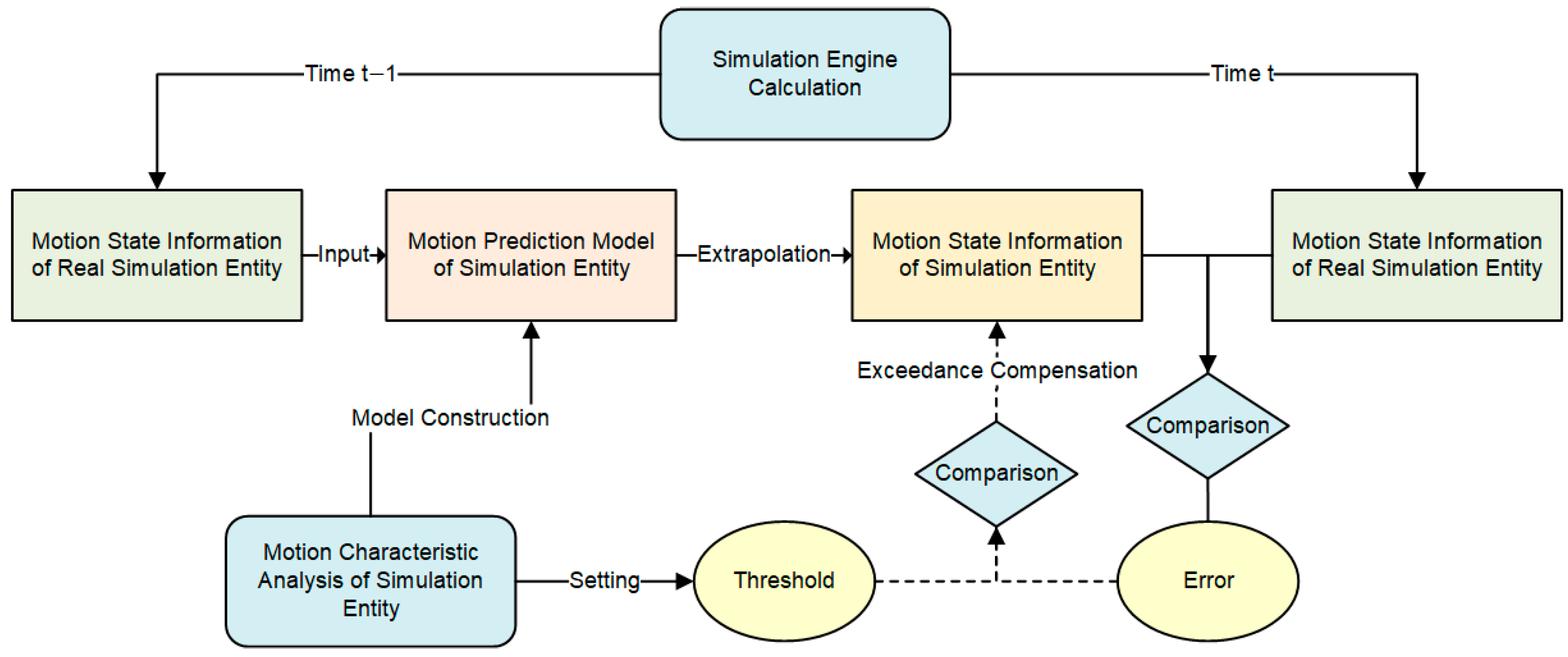
Dead Reckoning (DR) is a navigation technology that continuously estimates the current position, velocity, and heading of an object based on known initial motion states (initial position, velocity, heading) and motion laws [15,16]. It is widely used in aviation, maritime navigation, robotic navigation, and pedestrian navigation [17,18,19]. The core of DR lies in updating the motion state through velocity vector integration, which does not require external signal support (e.g., GPS) and has the advantage of strong independence [20]. However, in long-duration or high-dynamic environments, prediction errors accumulate over time, affecting the reckoning accuracy [21,22]. Figure 1 shows the basic principle of the traditional DR algorithm.

The workflow of the traditional DR algorithm is as follows:

(1) Real data input: The simulation engine calculates and outputs the motion state information of the real simulation entity at time t − 1, which is input into the “motion prediction model of the simulation entity”.

(2) Motion state extrapolation: Based on the real state at time t − 1, the prediction model generates the “predicted motion state at time t” via extrapolation.

(3) Error generation: The predicted motion state is compared with the real state at time t (output by the simulation engine) to obtain the error between them.

(4) Error-threshold verification: The error is compared with the threshold set by “motion characteristic analysis of the simulation entity” to determine if it exceeds the tolerance range.

(5) Exceedance compensation: If the error exceeds the threshold, perform exceedance compensation is applied to the predicted motion state to ensure the final motion state meets accuracy requirements.

(6) Model construction: The motion characteristic analysis of the simulation entity also provides a basis for the construction of the prediction model, supporting the model to adapt to the motion rules of the simulation entity.

The traditional DR algorithm constructs a prediction model based on kinematic mechanisms which can meet the requirements of simple scenarios. However, for complex motion processes, it is difficult to accurately reflect the true motion state of the entity through mechanism abstraction and simplification. This leads to frequent threshold crossings of prediction errors, resulting in frequent information interaction among simulation nodes and failing to achieve the goal of reducing simulation delay.

2.2. Intelligent DR Algorithm

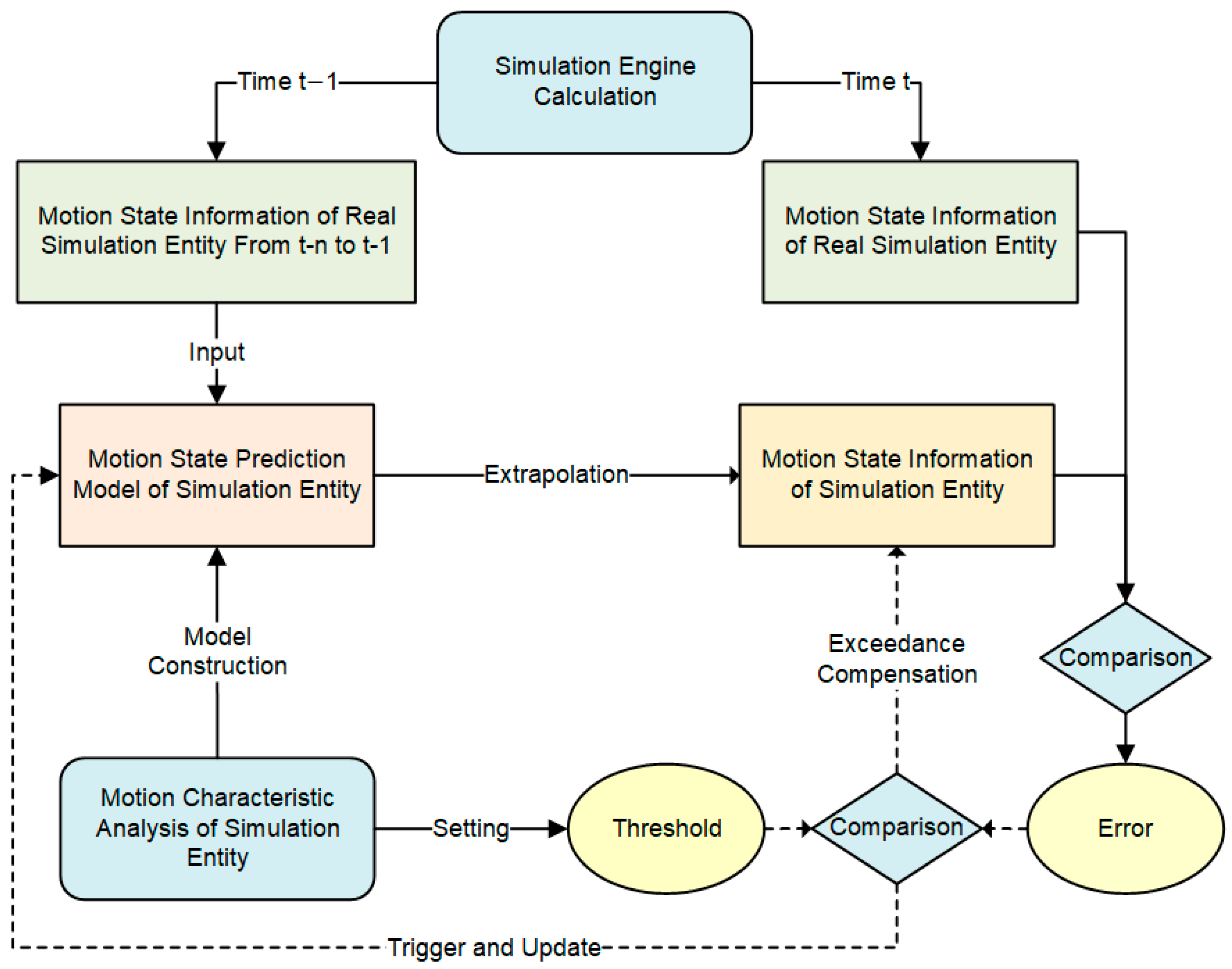
Deep neural networks possess strong capabilities in regards to automatic feature extraction, nonlinear relationship modeling, and capturing long-term dependencies, enabling the construction of data-driven models that are challenging to formulate mathematically. By establishing a feedback link between error data and the motion prediction model, the model parameters can be continuously updated, thereby improving prediction accuracy and reducing the frequency of information compensation updates. Figure 2 shows the basic principle of the intelligent DR algorithm.

The workflow of the intelligent DR algorithm is as follows:

(1) Model prediction: The historical real state is input into the prediction model, and the predicted motion state at time t is generated via extrapolation.

(2) Error verification: The predicted state is compared with the real state at time t to generate an error, and the error is compared with the “threshold set by motion characteristic analysis” to determine if it exceeds the limit.

(3) Dual-branch actions: If the error exceeds the threshold, then perform exceedance compensation on the predicted state to obtain a usable state.

(4) Meanwhile, the comparison result triggers “model update”: Reconstruct the prediction model based on motion characteristic analysis to optimize the next round of prediction.

(5) Cycle iteration: The optimized model is used for prediction at the next time step, forming a closed loop of “prediction-verification-compensation/update”.

3. Model Architecture Design

3.1. Core Components of the Model

To meet the demand for collaborative modeling of global motion dependencies and local time-series details in Dead Reckoning (DR), Transformer and LSTM are selected as core components. Through targeted improvements and adaptations, a foundation is laid for the subsequent construction of the hybrid model.

3.1.1. Transformer Component

The original Transformer captures global dependencies by introducing the self-attention mechanism [27]. Targeting the unidirectional dependency characteristic of DR time-series prediction, the following improvements are made to the original Transformer architecture:

(1) Architecture Streamlining and Adaptation: Remove the decoder attention layer of the original Transformer to block the bidirectional information interaction path at the structural level, thereby avoiding interference with the prediction logic caused by the leakage of future time-series information.

(2) Positional Encoding Optimization: Introduce a time decay factor to reconstruct the positional encoding mechanism, enhancing the model’s attention to recent time-series information and solving the problem introduced by the fact that traditional encoders make no distinction in weights between near and far time-series data. The formulas are as follows:

$$PE(pos,2k)=\sin \left({\displaystyle \frac{pos}{{\tau }^{2k/d_{emb}}}}\cdot \exp (-{\displaystyle \frac{pos}{T}})\right)$$

(1)

$$PE(pos,2k+1)=\cos \left({\displaystyle \frac{pos}{{\tau }^{2k/d_{emb}}}}\right)\cdot \exp \left(-{\displaystyle \frac{pos}{T}}\right)$$

(2)

where $pos$ represents the time-series position index of elements in the sequence, $k$ is the dimension index of the embedding vector, $\tau$ = 10,000, $d_{emb}$ is the feature embedding dimension, $T$ is the input sequence length, and $\exp \left(-pos/T\right)$ is the temporal attenuation factor, which is used to weight and emphasize the temporal importance of recent trajectory data. This design enables the model to distinguish the temporal order of sequence elements and emphasize recent data, which is crucial for capturing time-dependent motion patterns.

(3) Attention Mask Constraint: Design a lower triangular attention mask matrix $M$. The mask mechanism blocks the attention weight contribution of future time-series positions to the current prediction, completely eliminating the problem of time-series information leakage. The formula is as follows:

$$\mathrm{Self}\text{-}\mathrm{Attention}(Q,K,V)=\mathrm{Softmax}\left({\displaystyle \frac{Q{K}^T}{\sqrt{d_k}}}+M\right)V$$

(3)

where $d_k=d_{emb}/h$ ($h$ is the number of attention heads), and the scaling factor $\sqrt{d_k}$ is used to prevent the dot product result from becoming too large, which leads to the saturation of the softmax function and gradient vanishing. The mask $M$ satisfies $M_{i,j}=0$ when $j>i$ and $M_{i,j}=1$ when $j\le i$.

This component captures cross-time-series global motion dependencies through the Multi-Head Attention mechanism. It realizes nonlinear feature transformation via the Feed-Forward Network (FFN) and finally outputs a global motion feature vector, providing global feature support for the subsequent fusion module.

3.1.2. LSTM Component

The Long Short-Term Memory (LSTM) network employs its unique three-level gating mechanism, comprising the input gate, forget gate, and output gate, to accurately filter and enhance local sequence information across consecutive time steps, wherein the forget gate is responsible for screening and discarding redundant historical motion state information, the input gate selectively integrates key dynamic features of the current time step into the cell state, and the output gate generates a highly discriminative local time-series feature vector based on the updated cell state, which can accurately characterize the continuous maneuvering patterns of the target within short time periods.

Ultimately, the local time-series feature vector output by the LSTM forms a strong complementary relationship with the global correlation features output by the Transformer; the former ensures the modeling accuracy of instantaneous maneuver details, while the latter enhances the perception capability of long-sequence motion trends. Both are jointly fed into the subsequent feature fusion module, providing comprehensive feature support for the accurate prediction of target motion states.

3.2. Transformer–LSTM Hybrid Model

3.2.1. Model Structure

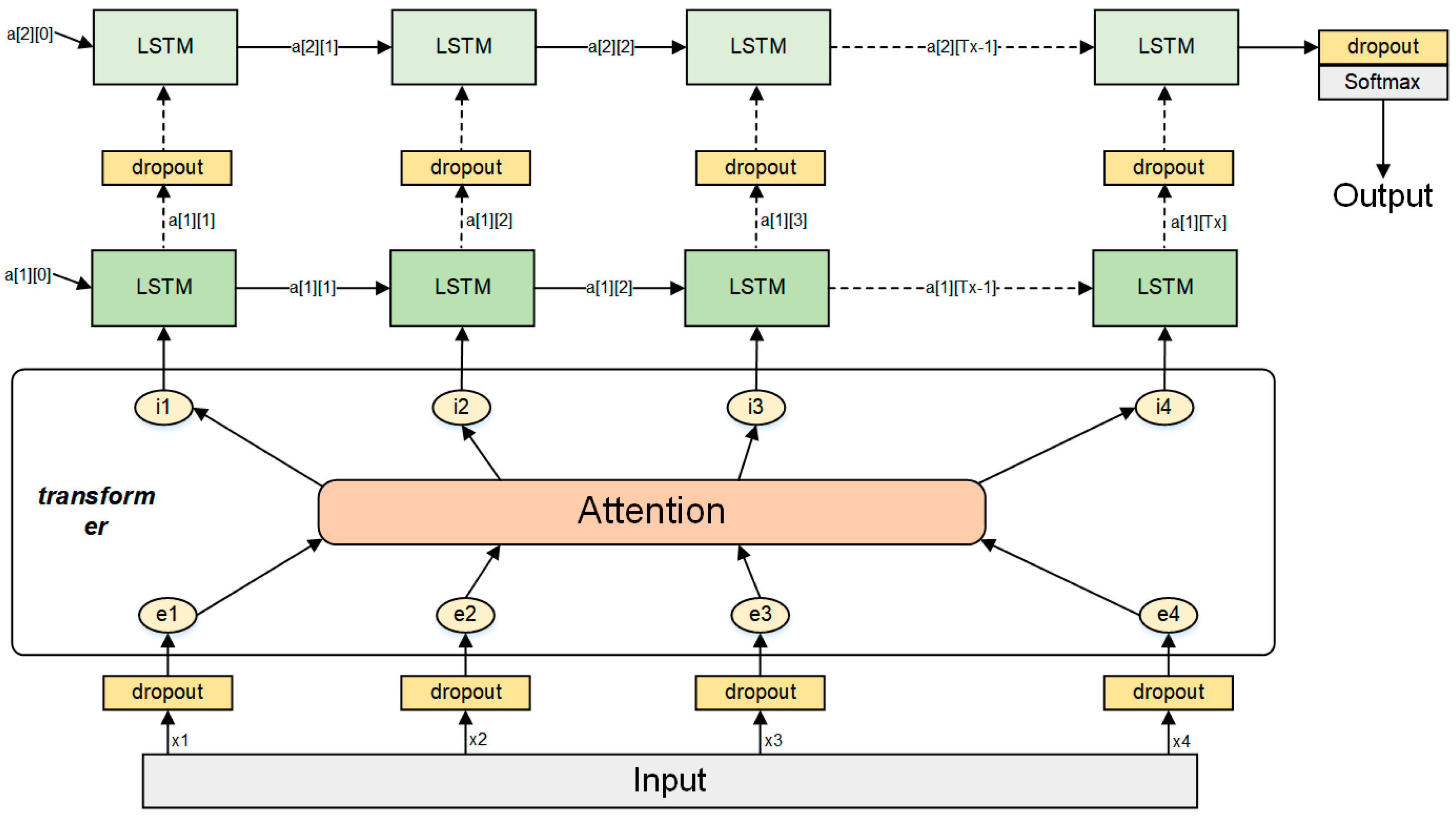
The Transformer–LSTM hybrid model integrates the modified Transformer and LSTM components based on their functional advantages, forming a targeted integration architecture rather than a simple stacking, as shown in Figure 3.

(1) Input Layer: The input data is a time-series motion sequence of simulation nodes, including position ($x, y, z$), velocity ($v_x,v_y,v_z$), acceleration ($a_x,a_y,a_z$), and heading $\theta$, with a total of 10 features. The sequence length is set to $le{n}_{seq}$ (i.e., using the motion data of the previous $le{n}_{seq}$ time steps to predict the state of the next time step, which is determined through cross-validation to balance prediction accuracy and computational efficiency.

(2) Embedding Layer: Convert the input sequence ($le{n}_{seq}$ × 10) into high-dimensional embedding vectors ($le{n}_{seq}$ × $d_{emb}$) through a fully connected layer, mapping low-dimensional motion features to high-dimensional space.

(3) Modified Transformer Encoder: Contains two encoder layers. Each encoder layer includes a Multi-Head Attention sub-layer (number of attention heads is $h$) and an FFN sub-layer. The Transformer encoder outputs global feature vectors ($le{n}_{seq}$ × $d_{emb}$) by capturing the global dependencies of the motion sequence.

(4) Feature Fusion Layer: The output of the Transformer encoder is normalized (LayerNorm) and then concatenated with the local temporal feature vectors (extracted by a 1D convolution layer with kernel size three) to form fused feature vectors ($le{n}_{seq}$ × $d_{emb}$), enhancing the model’s ability to capture both global and local features.

(5) LSTM Layer: Contains two LSTM layers with a configurable hidden layer dimension $d_{hidden}$ and a dropout rate $rat{e}_{dropout}$ to prevent overfitting. The LSTM layer processes the fused feature vectors, capturing long-term temporal dependencies in the motion sequence.

(6) Output Layer: A fully connected layer maps the output of the LSTM layer ($d_{hidden}$-dimensional) to the predicted motion state (10-dimensional, including position, velocity, acceleration, and heading at the next time step).

3.2.2. Workflow

The workflow of the hybrid model is as follows:

(1) The input motion sequence is converted into high-dimensional embedding vectors.

(2) The modified Transformer encoder performs global feature extraction and long-range dependency modeling, obtaining feature representations rich in global structural information.

(3) The feature fusion layer integrates global and local features, and the LSTM layer further captures long-term temporal dependency.

(4) The output layer generates the predicted motion state.

The entire process realizes the complementary advantages of Transformer and LSTM, improving the accuracy of motion state prediction.

3.3. Closed-Loop Feedback Update Mechanism

The closed-loop feedback update mechanism is tightly integrated with the Transformer-LSTM hybrid model. The error feedback signal ($Err$) triggers updates for key hyperparameters of the hybrid model, including the Transformer’s attention head number, LSTM’s hidden layer dimension, and so on; the parameter optimization process runs in parallel with model inference; when the update trigger condition is met, the optimization process uses idle resources to complete the local search, and the new parameters will be adopted in the next inference step.

3.3.1. Error Feedback Signal

As the input of the closed-loop mechanism, the error feedback signal $Err$ must fully reflect the prediction deviations of the model for all motion features, while highlighting the importance of key features through weighted distribution. Based on the previously defined 10-dimensional input motion features, $Err$ is defined as the weighted sum of the normalized errors of each feature, with the specific formula as follows:

$$Err={\displaystyle \sum _{j=1}^{10}{w}_j}\cdot {\displaystyle \frac{|y_j-{\widehat{y}}_j|}{{\sigma }_j}}$$

(4)

where $w_j$ is the feature weight coefficient, set according to the degree of influence of different features on motion state prediction: position features with $w=0.4$, velocity features with $w=0.3$, acceleration features with $w=0.2$, and heading angle features with $w=0.1$; ${\sigma }_j$ comprise the standard deviation of the j-th feature in the training set, used to eliminate the dimensional difference between different features; $y_j$ is the true value of the j-th feature; and ${\widehat{y}}_j$ is the model’s predicted value. This design not only ensures the dimensional unity of the error signal but also enhances the error sensitivity of core features such as position and velocity through weight distribution, ensuring that the feedback signal can accurately reflect the model’s prediction performance.

3.3.2. Parameters to Be Updated

The hyperparameters of the Transformer–LSTM model subject to optimization, along with their predefined search ranges, are detailed in

Table 2. Optimized hyperparameters and search ranges.

Hyperparameter	Description	Search Range
$d_{emb}$	Transformer embedding dimension	[128, 256, 512]
$h$	Number of Transformer attention heads	[2, 4, 8]
$d_{hidden}$	LSTM hidden layer dimension	[128, 256, 512]
$lr$	Learning rate	[1 × 10−5, 1 × 10−4, 5 × 10−4, 1 × 10−3]
$rat{e}_{dropout}$	Dropout rate	[0.1, 0.2, 0.3, 0.4, 0.5]
$le{n}_{seq}$	Input sequence length	[20, 30, 40]

. The selection of these parameters critically influences the model’s prediction accuracy and computational efficiency.

3.3.3. Update Trigger Conditions

The design goal of the update trigger mechanism is to balance model adaptation sensitivity and computational resource overhead, avoiding excessive updates that affect simulation real-time performance while preventing error accumulation caused by delayed updates. Based on the error distribution characteristics and simulation scenario requirements, dual trigger conditions are set (satisfying either one is sufficient), and all thresholds are determined through 3-fold cross-validation combined with statistics of 100,000 sample sets, as follows:

(1) Feedback error exceeding threshold condition: Feedback error $Err>0.15$. Statistical analysis shows that the $Err$ of the vast majority of normal prediction samples is concentrated below 0.15, and $Err$ will only exceed this threshold when the model encounters unlearned complex maneuver patterns (such as sudden high-G turns or composite maneuver switching). Triggering an update at this time can quickly adapt to new motion laws and avoid continuous error expansion; the threshold of 0.15 balances sensitivity and stability, neither causing frequent updates due to an excessively low threshold nor resulting in adaptation lag due to an excessively high threshold.

(2) Excessively fast cumulative error growth condition: The growth rate of cumulative error over five consecutive time steps exceeds 20%. The mathematical expression is

$$Er{r}_{sum}(t)={\displaystyle \sum _{k=t-4}^{t}Err}(k)$$

(5)

$${\displaystyle \frac{Er{r}_{sum}(t)-Er{r}_{sum}(t-5)}{Er{r}_{sum}(t-5)}}>20\%$$

(6)

where $Err(k)$ is the feedback error at time step $k$, and $Er{r}_{sum}(t-5)$ is the cumulative error of the five time steps before the current window. The $Err$ of a single time step may occasionally exceed the threshold due to random noise (such as sensor disturbance), while cumulative error growth can reflect the trending deterioration of errors (such as continuous changes in target motion patterns). Choosing five time steps balances response speed and anti-interference ability; the 20% growth rate threshold is determined by comparing the error change rates under different maneuver scenarios, ensuring that updates are only triggered when the model performance significantly declines.

3.3.4. Operational Logic

The operational process of the closed-loop error feedback-parameter update mechanism follows the logic of “real-time monitoring-trigger judgment-optimization update-cyclic iteration”, with specific steps as follows:

(1) Error calculation: After the model completes each motion state prediction, the feedback error, calculate $Err$ by weighting the motion features, and record the $Err$ sequence of consecutive time steps to provide data support for judging cumulative error growth.

(2) Trigger judgment: Based on the dual update trigger conditions and fallback rules, determine whether to initiate parameter update. If either trigger condition is met, enter the parameter optimization process; otherwise, continue prediction using the current hyperparameters.

(3) Local optimization: Start the preset meta-heuristic optimization algorithm for local hyperparameter optimization, taking the current optimal hyperparameter combination as the initial value and limiting the number of iterations to a reasonable range. This process usually focuses on the optimal parameter interval corresponding to the current motion pattern, achieving parameter adaptation through local fine-tuning, avoiding the high computational overhead caused by global search, and ensuring simulation real-time performance.

(4) Parameter update: Replace the current model parameters with the optimal hyperparameter combination obtained from optimization to complete one closed-loop update; subsequently, the model performs the next round of prediction based on the new parameters, continuously cycling through the above process to achieve adaptive adaptation to dynamic motion patterns.

4. Model Parameter Optimization

4.1. Principles of the PLO Algorithm

Polar Lights Optimization (PLO) is a novel meta-heuristic intelligent optimization algorithm inspired by the formation and variation process of polar lights. Its core operating steps include three key phases, which balance global exploration and local exploitation to achieve efficient parameter optimization.

(1) Initialization phase: A particle swarm is randomly generated within the predefined search range of hyperparameters, where each particle represents a unique combination of hyperparameters.

(2) Iteration phase: Three core motion mechanisms drive particle updates. First, gyration motion enables local fine-tuning near the current optimal solution to refine parameter combinations; then, auroral oval walk supports global search by allowing particles to move rapidly around candidate optimal points; finally, particle drift and diffusion introduce random disturbances to avoid premature convergence.

The iteration terminates when the maximum number of iterations is reached or the fitness value converges (with minimal changes over consecutive iterations).

Compared with traditional optimization algorithms such as Particle Swarm Optimization (PSO) and Genetic Algorithm (GA), PLO exhibits stronger global search capability and faster convergence speed, making it particularly suitable for hyperparameter tuning of the Transformer–LSTM hybrid model in Dead Reckoning (DR) scenarios. It effectively adapts to diverse maneuver patterns in distributed interactive simulation (DIS) and ensures that the model obtains optimal hyperparameter combinations.

4.2. Algorithm Framework

The framework of the PLO algorithm for optimizing the Transformer–LSTM model is shown in Algorithm 1.

Algorithm 1. PLO
PLO pseudocode
	Input: maximum number of iterations $T$ collision probability $K$ gyration frequency $\omega$, the number of particles $N$, the number of optimized hyperparameters $D$. Output: optimal hyperparameter combination $g_{best}$.
	1. Initialize the particle swarm $X(N, D)$
	2. For each particle i in the swarm
		Initialize the model with the hyperparameter combination $X_i$.
		Train the model on the training set.
		Calculate the fitness value.
	3. Record the individual optimal position $p_i$ and the global optimal position $g_{best}$ of the swarm
	5. While $t < T$ do
		For each particle $i$ in the swarm
			Calculate $W_1$ (the weight of the gyration motion) and $W_2$ (the weight of the auroral oval walk)
			Update the position of particle i using the gyration motion and auroral oval walk
			If $rand\left(0,1\right) < K$ Update the position of particle i using the particle drift and diffusion mechanism
			Clip the position of particle i to the search range of each hyperparameter
			Train the model with the new hyperparameter combination, calculate the fitness value
			If the current fitness value is less than $p_i$’s fitness value, update $p_i$ to the current position
		Update $g_{best}$ to the position of the particle with the minimum fitness value in the swarm
		$t=t+1$
	6. Return the global optimal position $g_{best}$ as the optimal hyperparameter combination of the model

4.3. PLO Optimization Process Verification

4.3.1. Fitness Function Design

The fitness function is used to evaluate the quality of hyperparameter combinations, which is defined as the MSE of the DR prediction results on the validation set, as follows:

$$\mathrm{Fitness}={\displaystyle \frac{1}{N\times M}}{\displaystyle \sum _{i=1}^N{\displaystyle \sum _{j=1}^M{(y_{ij}-{\widehat{y}}_{ij})}^2}}$$

(7)

where $N$ is the number of samples in the validation set, $M$ is the number of predicted features ($M$ = 10), $y_{ij}$ is the true value of the j-th feature of the i-th sample, and ${\widehat{y}}_{ij}$ is the predicted value. Under the premise of satisfying real-time constraints, a smaller fitness value indicates better model performance.

4.3.2. Sensitivity Analysis of PLO Parameters

To verify the rationality of PLO parameter settings, sensitivity analysis is performed on key parameters ($N,T,K$) as follows:

(1) When $N$ increases from 20 to 30, the optimal fitness value decreases by 12.3%; when it increases to 40, the fitness value only decreases by 2.1%, while the sample prediction time increases significantly. Thus, $N$ = 30 is selected.

(2) When $T$ increases from 80 to 100, the fitness value decreases by 8.7%; when it increases to 120, the fitness value remains basically unchanged, but the prediction time is longer. Thus, $T$ = 100 is selected.

(3) When $K$ = 0.2, the model’s effect of avoiding premature convergence is better than that when $K$ = 0.1 (with a 7.5% lower fitness value) and $K$ = 0.3 (with a 4.2% lower fitness value). Thus, $K$ = 0.2 is selected.

4.3.3. Convergence Curve Comparison

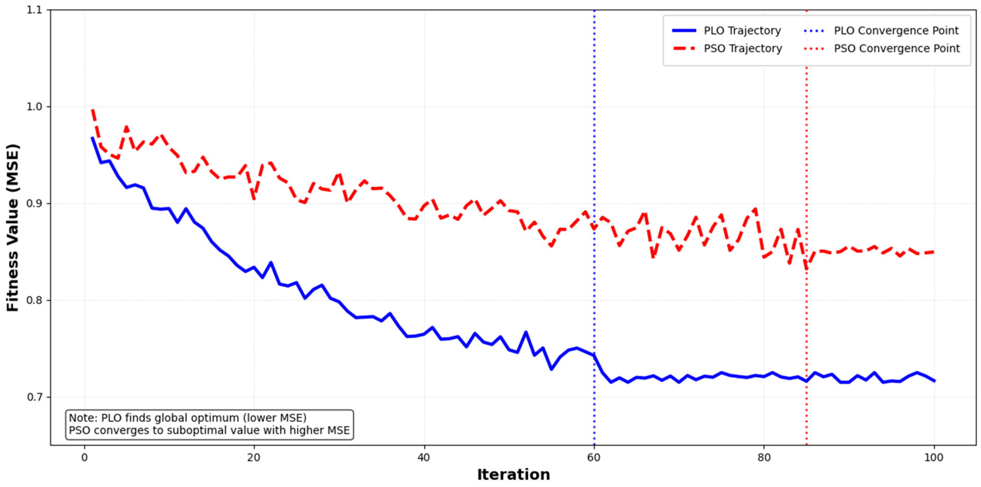
Figure 4 shows the convergence curves of PLO and PSO. PLO converges at approximately 60 iterations, while PSO converges at 85 iterations, indicating that PLO’s convergence speed is 30.6% faster than that of PSO. The final optimal fitness value of PLO is 0.72, which is 15.3% lower than PSO’s 0.85.

4.3.4. Parameter Evolution Trajectory

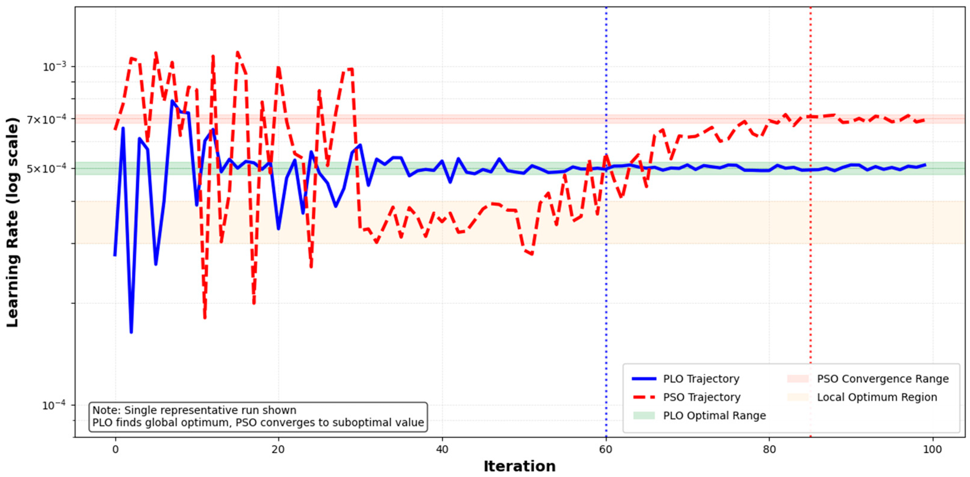
Figure 5 shows the evolution trajectory of the learning rate (a key hyperparameter). PLO initially explores a wide range (1 × 10⁻⁵, 1 × 10⁻³) and quickly converges to the optimal range (4.8 × 10⁻⁴, 5.2 × 10⁻⁴). In contrast, PSO falls into local optima at iterations of 30~50, with a final learning rate deviating from the optimal value.

4.3.5. Optimization Stability Comparison

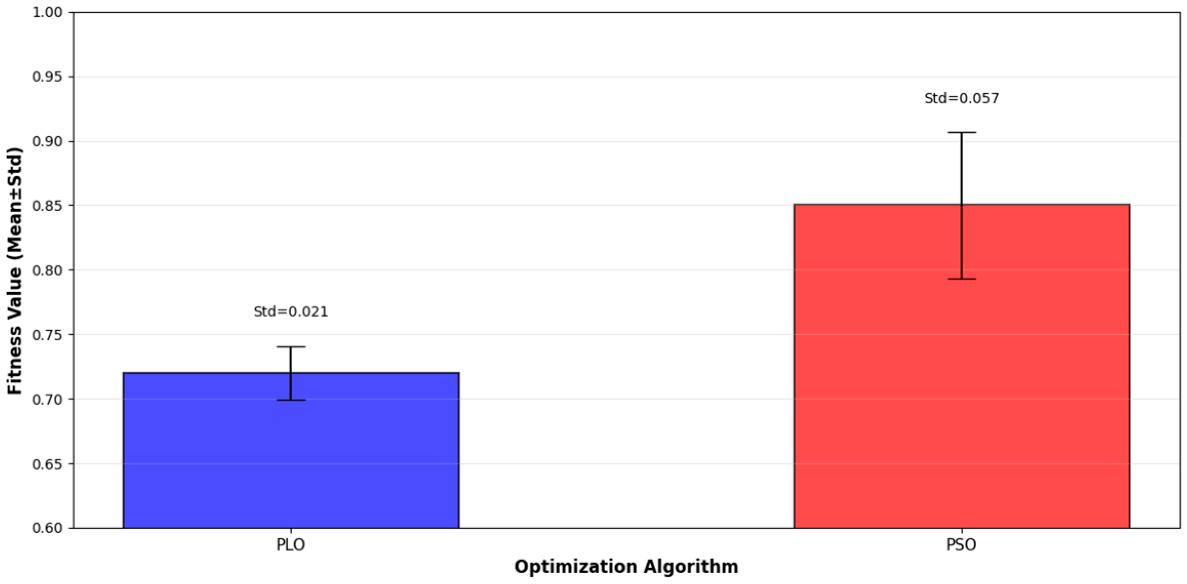
Figure 6 shows the stability metrics of PLO and PSO in five independent optimization runs. PLO displays a smaller fitness value standard deviation (0.021 vs. 0.057) and a narrower hyperparameter fluctuation range, verifying its stronger stability.

4.3.6. Final Optimal Hyperparameters

Based on the PLO optimization process verification, the final optimal hyperparameter combination of the Transformer–LSTM hybrid model is determined as follows: the Transformer embedding dimension = 256, the number of Transformer attention heads = 4, the LSTM hidden layer dimension = 256, the learning rate = 5 × 10⁻⁴, the dropout rate = 0.3, and the input sequence length = 30.

This combination fully balances prediction accuracy and computational efficiency. The 256-dimensional embedding and hidden layer dimensions ensure sufficient feature expression capability without excessive computational overhead; the four attention heads enable the effective capture of global motion dependencies while controlling model complexity; the 5 × 10⁻⁴ learning rate achieves fast convergence and stable training (verified by the learning rate evolution trajectory in Figure 5); the 0.3 dropout rate suppresses overfitting (adapted to the noise characteristics of the maneuvering dataset); and the 30-step input sequence length covers the key time window of target maneuvering, providing sufficient historical information for prediction.

5. Experimental Verification

5.1. Experimental Design

5.1.1. Experimental Scenario

The experiment uses the complex maneuvering processes of three aerial targets (A, B, C) as the test scenario and constructs a high-fidelity, reproducible distributed simulation verification environment to support the training and evaluation of the DR model. On this basis, target A is selected as the typical validation subject, and a specific scenario covering the entire process of extreme maneuvering–normal cruise-cooperative avoidance is designed (Figure 7).

(1) Extreme large-angle climb/dive: Simulating the strong nonlinear maneuver process of the short-distance penetration of flight targets, large-angle attitude adjustment and high-overload vertical acceleration were set to focus on testing the model’s adaptability to dynamic mutation scenarios. The parameter design is as follows: The displacement in the X direction ranges from 0 to 10,000 m, there is no lateral offset in the Y direction (fixed at 0), and the Z direction completes a climb from 0 to 6000 m altitude, followed by a dive to 3000 m; the corresponding average climb angle is approximately 50°, the average dive angle is approximately 45°, and the vertical acceleration is controlled at ±5~6 G. This scenario focuses on verifying the model’s adaptability to dynamic mutation scenarios.

(2) Conventional small-angle cruising: Simulating the stable movement process of the long-distance cruising of flight targets, the small-amplitude lateral offset and altitude elevation were set to focus on verifying the model’s ability to suppress error accumulation under long-time sequence operating conditions. The parameter design is as follows: the displacement in the X direction ranges from 10,000 m to 30,000 m, the Y direction gently offsets from 0 to 600 m, and the Z direction slightly rises from 3000 m to 3200 m; the turning angle is approximately 3°, and the cruising speed remains stable. This scenario focuses on verifying the model’s ability to control the error accumulation effect under conventional operating conditions.

(3) Snake-like evasive maneuver: Simulating the multi-group S-type series maneuver process of flight targets evading interception, a time-series coupled scenario was constructed through reciprocating lateral fluctuations and vertical undulations to focus on verifying the model’s fitting accuracy of the coupled parameters and the interference elimination capability. The parameter design is as follows: The displacement in the X direction ranges from 30,000 m to 40,000 m, the Y direction fluctuates reciprocally based on 600 m (fluctuation range ±500 m), and the Z direction undulates, with 3200 m as the benchmark (fluctuation range ±500 m); the turning angle is ±25°, and a total of five groups of S-turns are distributed within a 10 km distance. This scenario focuses on verifying the model’s fitting accuracy of the time-series coupled parameters.

Furthermore, a full-process continuous composite maneuver integrating the above three types of scenarios, i.e., a complete movement link in the X direction from 0 to 40,000 m, was formed to realize the smooth switching of “climb–dive–cruise–snake-like” maneuvers, focusing on verifying the long-term prediction stability of the model employing the alternation of complex continuous operating conditions.

5.1.2. Experimental Platform Configuration

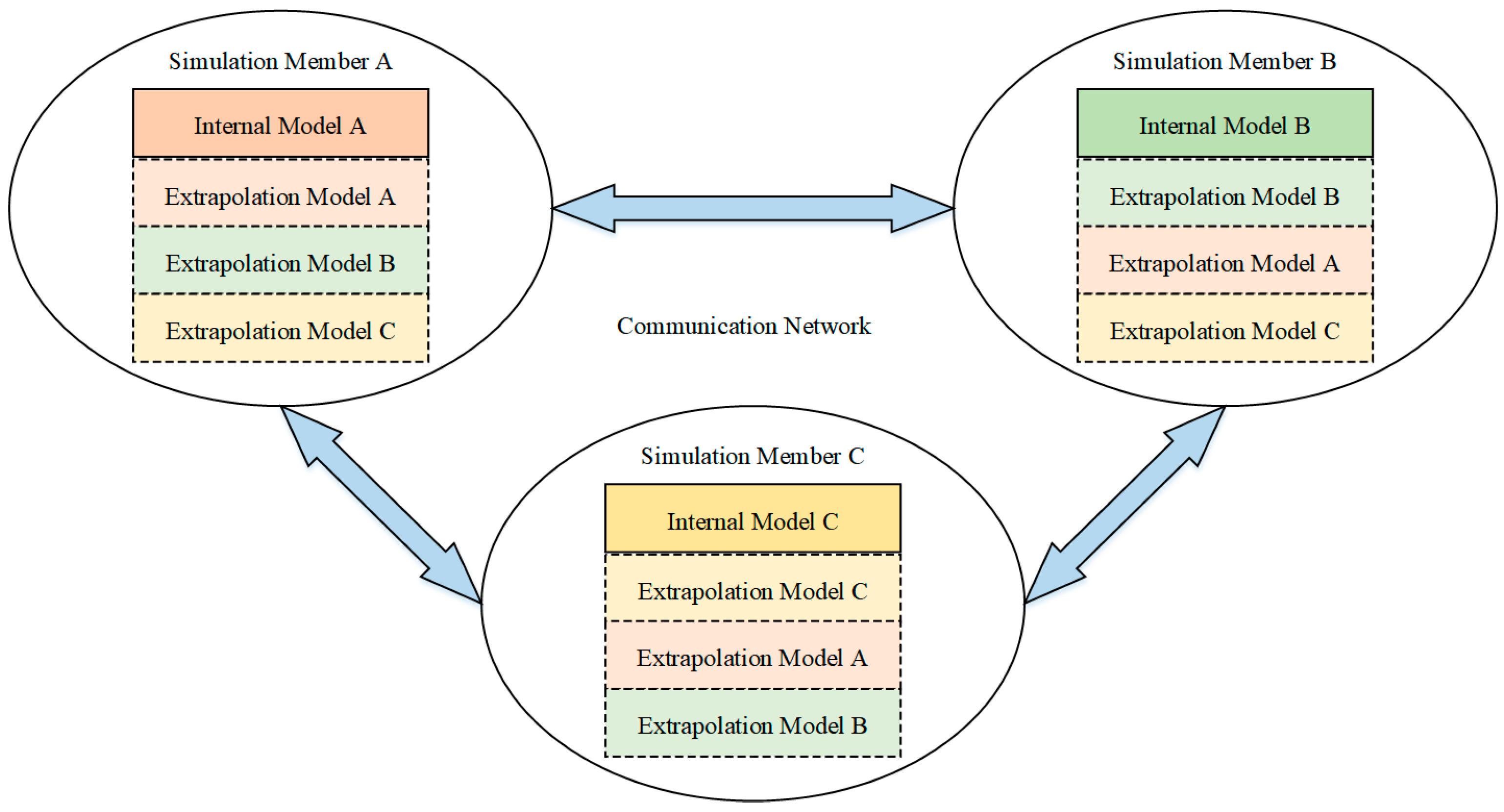
To verify the superiority of the DR algorithm based on the PLO–Transformer–LSTM model, a distributed interactive simulation experimental environment consistent with Figure 8 was constructed. Taking simulation member A as an example, A’s internal model reflects the true motion state of target A, and A’s extrapolation model reflects the estimated state of fighter A. During the maneuver, if the state information deviation between A’s internal and A’s extrapolation is not significant, then A’s extrapolation information does not need to be updated to the true value. Only when the deviation exceeds a certain threshold will A’s extrapolation initiate an update and send the relevant information synchronously to members B and C.

The experimental platform for simulation nodes A, B, and C is uniformly configured as follows:

(1) Hardware: Intel Core i7-13700K CPU (3.4 GHz), NVIDIA RTX 4090 GPU (24 GB GDDR6X), 64 GB DDR5 RAM (4800 MHz).

(2) Operating System: Ubuntu 22.04 LTS (64-bit).

(3) Software: Python 3.11 (PyTorch 2.1.0, CUDA 12.1, NumPy 1.26.0, SciPy 1.11.4) for PLO–Transformer–LSTM model training and PLO optimization algorithm implementation; AFSIM v2.9 (an air and space simulation tool) was employed to model the motion of and generate trajectory data for the complex maneuvering targets [28], and the precision of its generated motion states is well-established within the aviation simulation community.

(4) Network: 10 GbE Ethernet (latency < 1 ms that follows a uniform distribution in the range of [0.1 ms, 1 ms]) with TCP/IP protocol for real-time node communication, which is consistent with the actual latency characteristics of distributed interactive simulation systems.

(5) Dataset: The target motion data were generated based on realistic aerial maneuver templates, including position, velocity, acceleration, and heading angle, with random perturbations added as needed to simulate real motion noise. The dataset was divided into a training set (70%), a validation set (15%), and a test set (15%). The training set was used for model parameter training, the validation set was applied for the hyperparameter tuning of PLO optimization, and the test set was utilized for the independent evaluation of model generalization ability. To eliminate dimensional differences among features, all data were normalized to the range of [0, 1] using the min-max normalization method.

5.1.3. Comparison Models

The following five types of mainstream models were selected for comparison to cover the technical routes, including traditional mechanism-driven, single deep learning; hybrid deep learning; and different intelligent optimization algorithm-assisted approaches, ensuring fair comparison among all models:

(1) Traditional EKF model: A classic mechanism-driven DR algorithm using a constant acceleration motion model as the state transition equation. The process noise covariance $\mathrm{Q}$ and observation noise covariance $\mathrm{R}$ were set through cross-validation, and the data were synchronized using min-max normalization.

(2) Pure LSTM model: Consistent in structure with the LSTM layer in the proposed model (two layers, hidden dimension is 256), with hyperparameters optimized via grid search with 3-fold cross-validation.

(3) Pure Transformer model: Consistent in structure with the modified Transformer encoder in the proposed model (two layers, embedding dimension is 256, number of attention heads is 4), with hyperparameters optimized via grid search with 3-fold cross-validation.

(4) PSO–Transformer–LSTM model: Identical in structure to that of the proposed model but using Particle Swarm Optimization (PSO) instead of PLO for hyperparameter tuning (PSO parameters: number of particles is 30, maximum iterations is 100, inertia weight is 0.7, acceleration coefficient is 2.0).

(5) PLO–Stacked Transformer–LSTM model: A comparative model with simple sequential connection (Transformer encoder–fully connected layer–LSTM layer, no feature fusion layer). Hyperparameters are optimized via PLO with the same search range as that of the proposed model.

5.1.4. Evaluation Metrics

(1)

Prediction accuracy metric

Overall accuracy: Mean Squared Error (MSE), Root Mean Squared Error (RMSE), Mean Absolute Error (MAE), Mean Absolute Percentage Error (MAPE), and coefficient of determination (R²).

Single-feature error: position error (Euclidean distance of x/y/z coordinates, unit: m), velocity error (unit: m/s), acceleration error (unit: G), and heading angle error (unit: °), focusing on the prediction performance of core motion features.

Weighted comprehensive error: Weighted sum of normalized errors of each feature (Formula (4)), reflecting the actual error judgment logic of DR.

(2)

Real-time performance metric

Average prediction time per sample (ms), reflecting computational efficiency, statistically based on GPU batch processing with batch size 32 and mixed precision training (FP16).

(3)

Communication overhead metric

Information interaction frequency among simulation nodes (times/s): triggered when the position error exceeds the preset threshold of 1 m, calculated as (number of threshold-exceeding time steps/total number of time steps) × 100 Hz (time step frequency). Position error calculation formula is

$$\mathit{PosErr}=\sqrt{{(x-\widehat{x})}^2+{(y-\widehat{y})}^2+{(z-\widehat{z})}^2}$$

(8)

where $x,y,z$ are the true position coordinates, and $\widehat{x},\widehat{y},\widehat{z}$ are the predicted position coordinates.

Position error threshold-exceeding ratio: percentage of time steps where position error exceeds the preset threshold (1 m), calculated as (number of threshold-exceeding time steps/total number of time steps) × 100%, reflecting the probability of triggering synchronization.

(4)

Computational complexity metric

Number of model parameters (Params) and floating-point operations per second (FLOPs), reflecting the model’s resource consumption.

(5)

Robustness evaluation metric

Noise sensitivity: R², MSE, and node synchronization frequency under different noise intensities, quantifying the model’s anti-interference ability.

Threshold sensitivity: R², MSE, and node synchronization frequency under different error thresholds, verifying the model’s ability to balance accuracy and communication overhead.

5.1.5. Training Configuration

All deep learning models were implemented using PyTorch 2.1.0 and optimized with the AdamW optimizer. Training proceeded for a maximum of 200 epochs, with early stopping (patience is 20 epochs) monitored on the validation loss. A batch size of 32 was used throughout. The loss function was Mean Squared Error (MSE). To ensure statistical significance, all experiments were repeated three times with different random seeds, and the reported results are the mean. The PLO and PSO optimization processes were also run independently three times, and the best-performing hyperparameter set was selected for final evaluation.

5.2. Results and Analysis

5.2.1. Model Performance Verification

To verify the multi-parameter collaborative fitting capability and working condition adaptability of the PLO model, the performance of the proposed model is evaluated against the traditional EKF baseline across the three maneuver scenarios described in Section 5.1.1 (Figure 8), and the results are summarized in

Table 3. Performance comparison of DR models in composite maneuver scenarios.

Maneuver Scenario	Evaluation Indicator	Traditional EKF Model	Intelligent DR Model	Error Reduction Rate
Extreme large-angle climb/dive	Average position error (m)	22.3	3.8	83.0%
	Average climb velocity error (m/s)	18.5	2.7	85.4%
	Average climb acceleration error (G)	1.5	0.18	85.0%
	Average heading angle error (°)	8.5	1.3	84.7%
	weighted comprehensive error	15.7	2.1	86.6%
Conventional small-angle cruising maneuver	Average position error (m)	8.6	1.8	79.1%
	Average climb velocity error (m/s)	9.2	1.2	87.0%
	Average climb acceleration error (G)	1.5	0.08	84.0%
	Average heading angle error (°)	3.5	0.5	85.7%
	weighted comprehensive error	7.8	1.1	85.9%
Snake-like evasive maneuver	Average position error (m)	24.2	4.1	83.1%
	Average climb velocity error (m/s)	20.1	3.0	85.1%
	Average climb acceleration error (G)	1.1	0.15	86.4%
	Average heading angle error (°)	9.2	1.2	86.9%
	Weighted comprehensive error	16.3	2.2	86.5%
composite maneuver	Weighted comprehensive error	14.9	1.9	84.5%

. In the three independent maneuver scenarios and the full-process continuous composite maneuver, all evaluation indicators of the proposed model are significantly better than those of the traditional EKF model. Among them, the reduction range of single-item errors is generally between 79% and 87%, and the reduction range of weighted comprehensive errors is stably between 84.5% and 86.6%. Moreover, the advantages are more prominent in extreme maneuver and snake-like evasive scenarios with strong nonlinearity and high coupling, which fully verifies the adaptability and prediction accuracy advantages of the model under different flight operating conditions.

5.2.2. Prediction Accuracy Comparison

Table 4. Prediction accuracy metrics of each model.

Model	MSE	RMSE	MAE	MAPE (%)	${\mathit{R}}^2$
Traditional EKF	1.24	1.11	0.94	2.08	0.779
Pure LSTM	0.93	0.96	0.76	1.65	0.887
Pure Transformer	0.98	0.99	0.81	1.73	0.880
PSO–Transformer–LSTM	0.85	0.92	0.67	1.45	0.931
PLO–Stacked Transformer–LSTM	0.82	0.90	0.71	1.52	0.925
PLO–Transformer–LSTM	0.72	0.85	0.58	1.23	0.962

presents the prediction accuracy metrics of each model for the test set, with all data satisfying the mathematical logic of a negative correlation between $MSE/R^2$, $RMSE=\sqrt{MSE}$ and consistent trends between MAE/MAPE. The key observations are as follows:

(1) The proposed PLO–Transformer–LSTM model achieved the best performance across all metrics, with goodness of fit reaching excellent levels in the field.

(2) Compared with the traditional EKF model, the proposed model reduced MSE by 42% ((1.24 − 0.72)/1.24 ≈ 0.419), MAE by 38%, RMSE by 39%, MAPE by 41% and increased $R^2$ by 0.183, significantly breaking through the limitations of traditional mechanism models relying on preset motion assumptions.

(3) The pure LSTM ($MSE$ = 0.93, $R^2$ = 0.887) and pure Transformer ($MSE$ = 0.98, $R^2$ = 0.880) models exhibited similar performance, both of which were lower than that of the hybrid models, verifying the complementary effect of “global dependency capture + local temporal modeling”; the pure Transformer had a slightly lower $R^2$ than that of the pure LSTM due to its neglect of local maneuvering details.

(4) The proposed model reduced MSE by 15.3% compared with the results for the PSO–Transformer–LSTM model ((0.85 − 0.72)/0.85 ≈ 0.153), demonstrating that the PLO algorithm outperforms PSO in global search capability and convergence speed, enabling better hyperparameter combinations.

(5) The PLO–Stacked Transformer–LSTM model has an MSE of 0.82, which is 12.7% higher than that of the proposed model, verifying the superiority of the targeted integration strategy over simple stacking.

5.2.3. Ablation Experiment

To verify the contribution of each core component (modified Transformer, LSTM, PLO) of the model, ablation experiments were designed. All ablation models use the same hyperparameter search space (shown in

Table 5. Ablation experiment results.

Model	Configuration	MSE	${\mathit{R}}^{\mathbf{2}}$	MSE Change Rate vs. Proposed Model
Proposed Model	Transformer + LSTM + PLO	0.72	0.962	-
Model 1	LSTM + PLO (w/o Transformer)	0.85	0.903	+18.1%
Model 2	Transformer + PLO (w/o LSTM)	0.89	0.891	+23.6%
Model 3	Transformer + LSTM + Grid Search (w/o PLO)	0.89	0.885	+23.6%

) and optimization strategy (PLO, except Model 3 uses grid search) to ensure fair comparison.

(1) Model 1: With an MSE of 0.85 (8.6% lower than that of the pure LSTM model at 0.93), this result indicates that the PLO optimization can enhance the performance of a single model. However, after removing the Transformer’s global dependency capture capability, the MSE still increases by 18.1% compared to that of the Proposed Model. This verifies the necessity of the Transformer for predicting complex trajectory trends.

(2) Model 2: Achieving an MSE of 0.89 (9.2% lower than that of the pure Transformer model at 0.98), the PLO optimization similarly improves the performance of the single Transformer model. Nevertheless, the absence of LSTM’s local detail fitting leads to a 23.6% higher MSE than that of the Proposed Model, and its performance is inferior to that of Model 1. This highlights the core role of the Transformer in capturing global trends.

(3) Model 3: Although it achieved a similar MSE (0.89), its $R^2$ value (0.885) was lower than that of Model 2 (0.891). This result indicates that the grid search was less effective than PLO in optimizing the hyperparameters, as it was unable to locate the optimal combination. It further validates the superiority of the PLO algorithm in balancing global exploration and local exploitation.

5.2.4. Real-Time Performance Comparison

Table 6. Average prediction time per sample of each model.

Model	Average Prediction Time (ms/Sample)	FLOPs (G)	Computation Acceleration Method
Traditional EKF	0.02	0.001	CPU-only computation
Pure LSTM	0.35	1.8	GPU batch processing (batch size = 32)
Pure Transformer	0.38	2.1	GPU batch processing (batch size = 32)
PSO–Transformer–LSTM	0.42	3.1	GPU batch processing (batch size = 32)
PLO–Transformer–LSTM	0.43	3.2	GPU batch processing (batch size = 32)

shows the average prediction time per sample for each model, statistically based on GPU batch processing results. The key observations include the following:

(1) The traditional EKF model achieved the fastest prediction speed (0.02 ms/sample) due its reliance solely on mathematical formula recursion without complex neural network computations, making it suitable for scenarios with extreme real-time requirements (latency < 0.1 ms) but low accuracy demands.

(2) The pure LSTM and pure Transformer models exhibited similar prediction times (0.35 ms/sample and 0.38 ms/sample, respectively). The LSTM’s recurrent structure requires sequential computation by time step, resulting in general parallel efficiency; the Transformer’s multi-head attention mechanism supports parallel computation but has a slightly more complex layer structure, leading to comparable computational overhead between the two.

(3) The PSO–Transformer–LSTM and the proposed models had prediction times of 0.42 ms/sample and 0.43 ms/sample, respectively, only 0.05–0.08 ms longer than those for the pure models. Benefiting from the lightweight architecture (two layers for both Transformer and LSTM) + GPU parallel acceleration, the computational overhead is controllable. PLO optimization only affects the training process, without additional inference time costs.

(4) The proposed model comprises 2.8 M parameters and 3.2 G FLOPs, 133% more parameters than pure LSTM but only 77% more FLOPs, realizing a balance between accuracy and efficiency.

(5) The prediction time of all models was far below the real-time threshold (5 ms) in the DIS field. Even in scenarios with 1000 simultaneous entities, the total latency can be controlled within 20 ms through batch processing optimization, fully meeting engineering application requirements.

5.2.5. Communication Overhead Comparison

Table 7. Comparison of information interaction frequency among simulation nodes.

Model	Information Interaction Frequency (Times/s)	Position Error Threshold-Exceeding Ratio (%)	Interaction Frequency Reduction Rate vs. EKF
Traditional EKF	12.5	38	-
Pure LSTM	7.8	22	37.6%
Pure Transformer	7.5	21	40.0%
PSO–Transformer–LSTM	5.2	15	58.4%
PLO–Stacked Transformer–LSTM	5.5	16	56.0%
PLO–Transformer–LSTM	4.1	12	67.2%

presents the statistics for information interaction frequency and threshold-exceeding ratio among simulation nodes based on different models, with an error threshold of 1 m. The key observations include the following:

(1) The traditional EKF model had the highest interaction frequency (12.5 times/s) with a position error threshold-exceeding ratio of 38%. Due to a peak error of approximately 15 m, the threshold trigger mechanism was frequently activated, leading to excessive information interaction.

(2) The pure LSTM and pure Transformer models had interaction frequencies of 7.8 times/s and 7.5 times/s, respectively, representing reductions of 37.6% and 40.0% compared with the results for EKF, with the threshold-exceeding ratio decreasing to 22% and 21%, positively correlated with their error reduction rates (21–25%).

(3) The PSO–Transformer–LSTM model had an interaction frequency of 5.2 times/s, representing a 58.4% reduction compared with the results for EKF, with the threshold-exceeding ratio dropping to 15%, verifying the dual optimization effect of the hybrid architecture + intelligent optimization.

(4) The PLO–Stacked Transformer–LSTM model had an interaction frequency of 5.5 times/s, 25.5% higher than that of the proposed model, further confirming the advantage of the targeted integration strategy.

(5) The proposed model had the lowest interaction frequency (4.1 times/s), representing a 67.2% reduction compared with that of the EKF, with a threshold-exceeding ratio of only 12%. This result aligns with the core mechanism of DR algorithms: reduced errors directly decrease the number of threshold-exceeding triggers, and the impact of error peaks on interaction frequency is more significant in complex maneuvering scenarios (nonlinear correlation).

5.2.6. Robustness Experiment

(1)

Noise Sensitivity Analysis

To verify the robustness of the proposed model under noise interference, comparative experiments involving three noise intensity levels (variance = 0.1, 0.5, 1.0) were conducted. The anti-noise performance and communication overhead of different models were quantitatively evaluated, and the experimental results are summarized in

Table 8. Robustness experiment results under different noise intensities.

Noise Variance	Model	MSE	${\mathit{R}}^{\mathbf{2}}$	Synchronization Frequency (Times/s)
0.1	PLO–Transformer–LSTM	0.72	0.962	4.1
	PLO–Stacked Transformer–LSTM	0.82	0.941	5.3
	EKF	1.24	0.779	12.5
0.5	PLO–Transformer–LSTM	0.85	0.935	5.8
	PLO–Stacked Transformer–LSTM	0.98	0.912	6.7
	EKF	1.56	0.702	15.2
1.0	PLO–Transformer–LSTM	0.98	0.903	7.3
	PLO–Stacked Transformer–LSTM	1.15	0.885	8.2
	EKF	1.89	0.651	18.7

.

The coefficient of determination $R^2$ of the proposed PLO–Transformer–LSTM model remains above 0.90 across all noise intensity conditions: $R^2$ achieves 0.962 when the noise variance is 0.1 and still maintains a result of 0.903 even as the variance increases to 1.0. In contrast, the $R^2$ of the EKF model drops drastically to 0.651 under the strong interference condition, with a noise variance of 1.0, exhibiting a significantly higher performance degradation rate than that of the proposed model. These findings fully demonstrate that the proposed model possesses superior anti-noise interference capability.

From the perspective of the state synchronization frequency metric, as noise intensity increases, the synchronization frequency of the proposed model slightly rises from 4.1 times per second to 7.3 times per second, whereas that of the EKF model increases from 12.5 times per second to 18.7 times per second during the same period. Even under strong noise conditions, the state synchronization frequency of the proposed model is still significantly lower than that of the comparative models, thereby effectively retaining the technical advantage of low communication overhead.

(2)

Threshold Sensitivity Analysis

To verify the robustness of the proposed model across different error thresholds, comparative experiments involving four thresholds (0.5 m, 1.0 m, 1.5 m, 2.0 m) were conducted. The experimental results are summarized in

Table 9. Threshold sensitivity experiment results.

Threshold (m)	Model	MSE	${\mathit{R}}^2$	Synchronization Frequency (Times/s)
0.5	PLO–Transformer–LSTM	0.70	0.965	6.8
	PLO–Stacked Transformer–LSTM	0.80	0.928	8.2
	EKF	1.18	0.795	18.3
1.0	PLO–Transformer–LSTM	0.72	0.962	4.1
	PLO–Stacked Transformer–LSTM	0.82	0.925	5.5
	EKF	1.24	0.779	12.5
1.5	PLO–Transformer–LSTM	0.75	0.958	2.7
	PLO–Stacked Transformer–LSTM	0.88	0.912	3.6
	EKF	1.43	0.732	8.7
2.0	PLO–Transformer–LSTM	0.78	0.951	1.9
	PLO–Stacked Transformer–LSTM	0.95	0.898	2.5
	EKF	1.56	0.702	6.2

.

(1) As the threshold increases, the information interaction frequency of all models decreases, while the MSE slightly increases, reflecting the trade-off between prediction accuracy and communication overhead.

(2) The proposed model maintains a high $R^2$ (>0.9) across all thresholds. Its MSE increases from 0.70 to 0.78 (11.4% growth), which is lower than the EKF’s 32.3% growth and the PLO–Stacked model’s 18.3% growth; this verifies its strong robustness.

(3) At the threshold of 1.0 m, the proposed model achieves the optimal balance between accuracy ($R^2$ = 0.962) and communication overhead (4.1 times/s), which is the recommended threshold for engineering applications.

6. Discussion

6.1. Key Findings and Technical Implications

Based on the experimental results in Section 5.2, five core findings are derived, with significant technical implications for solving the bottlenecks of traditional DR algorithms in DIS.

(1) Hybrid architecture breaks through the limitations of single models: The complementary combination of “Transformer global dependency capture + LSTM local temporal modeling” effectively addresses the defects of pure models. This is because Transformer’s multi-head attention mechanism can capture long-range motion correlations, while LSTM’s gating mechanism filters local noise. Hybrid models achieve lower MSE and higher $R^2$ than do pure models, confirming this paradigm’s effectiveness for complex trajectory prediction.

(2) Targeted integration outperforms simple stacking: The proposed model’s MSE is 12.7% lower than that of the PLO–Stacked model, as the feature fusion layer realizes “global–local feature complementarity” rather than sequential connection. Specifically, the normalized Transformer global features and 1D convolution-extracted local features are concatenated, enabling the model to simultaneously focus on overall maneuver trends and sudden motion changes

(3) PLO optimization enhances model generalization: Compared with PSO, PLO’s gyration motion and auroral oval walk mechanisms balance local fine-tuning and global exploration. PSO easily falls into local optima in DR hyperparameter tuning (as shown in Figure 5), while PLO’s particle drift and diffusion avoid premature convergence, adapting to diverse maneuver patterns in DIS.

(4) Synergistic optimization of accuracy and communication overhead: The positive correlation between prediction accuracy and communication overhead reduction has been confirmed. DR triggers synchronization only when prediction errors exceed the threshold, so the hybrid architecture’s accurate motion state prediction directly reduces threshold-exceeding frequency. Meanwhile, PLO-optimized hyperparameters enhance model stability in complex maneuvers, avoiding error peaks that cause unnecessary interaction.

(5) Threshold sensitivity boosts engineering adaptability: The model maintains strong robustness across 0.5 m–2.0 m thresholds, thanks to the key design of the closed-loop mechanism. The model’s hyperparameters are dynamically adjusted according to threshold changes, i.e., tightening the threshold accelerates iteration to suppress small errors, while relaxing the threshold preserves stability and avoids excessive computation, thereby adapting to various DIS scenarios with different real-time/accuracy requirements.

6.2. Limitations and Future Directions

Despite the significant performance improvements, the proposed model still exhibits the following limitations that need to be addressed in future work:

(1) Poor performance in small-sample scenarios: The hybrid model relies on sufficient training data to learn maneuvering patterns. When the number of training samples is less than 3000, the $R^2$ decreases to below 0.90, and the MSE increases by more than 20%. Future work will explore transfer learning techniques, using pre-trained models on large-scale public datasets to improve adaptability in small-sample scenarios.

(2) Relatively high model complexity: The hybrid architecture (Transformer + LSTM) has a total of approximately 2.8 million parameters, which is higher than that of single models. Although GPU acceleration ensures real-time performance, it is not conducive to deployment on resource-constrained devices (e.g., embedded systems in unmanned aerial vehicles). Future research will focus on model lightweighting, such as reducing the number of layers through knowledge distillation or using sparse attention mechanisms to simplify the Transformer structure.

(3) Lack of multi-modal data fusion: The current model only uses motion sequence data (position, velocity, etc.) for prediction, without integrating other modal data (e.g., inertial sensor data, visual data). Multi-modal data can provide more comprehensive information to improve prediction robustness. Future work will explore multi-modal fusion strategies, such as using attention mechanisms to adaptively weight different modal features.

6.3. Engineering Application Prospects

(1) Aerial target simulation: It can be applied to the simulation of the complex maneuvering of fighter jets, drones, and other aerial targets, improving the accuracy of target state prediction and reducing communication overhead in distributed simulation systems. The complex motion pattern verification ensures its applicability in high-intensity combat simulation scenarios.

(2) Unmanned system coordination: For multi-unmanned vehicle/marine vehicle coordination scenarios, the model can reduce the frequency of information interaction between nodes, improving the real-time performance and stability of collaborative tasks. The threshold sensitivity analysis provides a flexible parameter adjustment scheme for different coordination latency requirements.

(3) Virtual reality (VR) simulation: In distributed VR systems (e.g., military training simulations), the model can reduce latency caused by network transmission, improving the immersion and interaction experience of users. The low communication overhead advantage is particularly prominent in large-scale multi-user VR scenarios.

In practical engineering applications, the model can be adjusted according to specific scenario requirements (e.g., adjusting the error threshold to balance accuracy and real-time performance, optimizing hyperparameters for specific maneuvering patterns), further enhancing its applicability.

7. Conclusions

To address the core bottlenecks of traditional Dead Reckoning (DR) algorithms in Distributed Interactive Simulation (DIS), such as their reliance on preset motion laws, limited prediction accuracy, and excessive communication overhead, this paper proposes a heuristic hybrid prediction model based on Polar Light Optimization (PLO). Through systematic experimental verification in complex air target maneuvering scenarios, the model achieves high-precision trajectory prediction with a goodness of fit (R²) exceeding 0.95. Compared with the results for the traditional Extended Kalman Filter (EKF) model, the Mean Squared Error (MSE) is reduced by 42%, and the state synchronization frequency of the simulation nodes is decreased by 67%. This achievement not only effectively reduces the communication resource consumption and simulation delay of the DIS system but also realizes the coordinated optimization of DR prediction accuracy and simulation real-time performance in complex maneuvering scenarios. It provides a technical solution with both theoretical innovation and engineering practicality for improving the temporal consistency of distributed interactive simulation and also offers a reusable modeling approach for similar dynamic target state prediction problems.

Compared with existing intelligent algorithm-driven DR methods, the innovations of this paper are threefold:

(1) The Transformer structure is modified for temporal prediction by removing the decoder attention layer and adding temporal logic constraints to positional encoding and attention computation, resolving the issue of temporal information leakage in trajectory data encountered by traditional encoder-only Transformers;

(2) The PLO optimization algorithm is introduced into DR model parameter tuning for the first time, and its superiority regarding convergence speed and stability is verified through process-level analysis;

(3) A closed-loop mechanism integrating error feedback and model parameter updating is established with clear mathematical formulation and operational logic, breaking through the limitations of traditional DR algorithms that only use real data for error compensation.

This research not only provides an efficient intelligent modeling method for the DR of complex moving targets but also offers a reference for accuracy optimization in other distributed simulation scenarios such as maritime navigation and ground unmanned systems. Nevertheless, the model still exhibits limitations in scenarios with insufficient data or extreme real-time requirements. Future work will further improve its engineering applicability through model lightweighting, multimodal data fusion, and cross-scenario transfer learning.

References

1. Di, Y. Design of Distributed Interactive Simulation Program Based on TENA. Microelectron. Comput. 2012, 29, 35–38. [Google Scholar]
2. Xu, C.; Song, J.; Chen, M.; Chen, J.; Yu, L. Research on Adaptive State Update Strategy of Distributed Interactive Simulation. In Proceedings of the 2011 Third International Conference on Multimedia Information Networking and Security, Shanghai, China, 4–6 November 2011; pp. 171–175. [Google Scholar] [CrossRef]
3. Zhang, X.; Ward, T.; Mcloone, S. Exploring an Information Framework for Consistency Maintenance in Distributed Interactive Applications. In Proceedings of the 2009 13th IEEE/ACM International Symposium on Distributed Simulation and Real Time Applications, Singapore, 25–28 October 2009; pp. 121–128. [Google Scholar] [CrossRef]
4. Durbach, C.; Fourneau, J.-M. Performance evaluation of a dead reckoning mechanism. In Proceedings of the 2nd International Workshop on Distributed Interactive Simulation and Real-Time Applications (Cat. No.98EX191), Montreal, QC, Canada, 20 July 1998; pp. 23–29. [Google Scholar] [CrossRef]
5. Yan, Z.; Chi, D.; Zhao, Z.; Deng, C. Dead reckoning error compensation algorithm of AUV based on SVM. In Proceedings of the OCEANS’11 MTS/IEEE KONA, Waikoloa, HI, USA, 19–22 September 2011; pp. 1–7. [Google Scholar] [CrossRef]
6. Su, T.L.; Kong, J.L.; Zhang, L.Y.; Jin, X.-B.; Bai, Y.-T.; Ma, H.-J. A Dead Reckoning Method Based on Neural Network Optimized Kalman Filter. In Proceedings of the 2022 IEEE International Conference on Unmanned Systems (ICUS), Guangzhou, China, 28–30 October 2022. [Google Scholar]
7. Kharitonov, V.Y. Motion-Aware Adaptive Dead Reckoning Algorithm for Distributed Virtual Reality Systems. In 32nd Computers and Information in Engineering Conference, Parts A and B, Proceedings of the ASME 2012 International Design Engineering Technical Conferences and Computers and Information in Engineering Conference, Chicago, IL, USA, 12–15 August 2012; ASME: New York, NY, USA; Volume 2, pp. 1473–1479. [CrossRef]
8. Meng, D.; Yao, Y.P.; Yao, F. An enhanced dead reckoning algorithm with hybrid extrapolation models (AisaSim 2016). Int. J. Model. Simul. Sci. Comput. 2017, 8, 1750027. [Google Scholar] [CrossRef]
9. Liu, D. An Improved DR Algorithm Based on Target Extrapolating in ROIA Cloud Platform. Int. J. Distrib. Sens. Netw. 2013, 9, 637328. [Google Scholar] [CrossRef]
10. Hou, X.; Bergmann, J. Pedestrian Dead Reckoning With Wearable Sensors: A Systematic Review. IEEE Sens. J. 2021, 21, 143–152. [Google Scholar] [CrossRef]
11. Kim, Y.; Ko, B.; Song, J. Magnetic Anomaly-Matched Trajectory and Dead Reckoning Fusion Mobile Robot Navigation. In Proceedings of the 28th International Conference on Artificial Life and Robotics, ICAROB 2023, Virtual, 9–12 February 2023. [Google Scholar]
12. Yu, K.; Li, K.; Liu, X.; Zhang, Q.; Feng, Z. Predictive Position Control for Movable Antenna Arrays in UAV Communications: A Spatio-Temporal Transformer-LSTM Framework. arXiv 2025, arXiv:2508.10720. [Google Scholar]
13. Ciabattoni, L.; Foresi, G.; Monteriù, A.; Pepa, L.; Pagnotta, D.P.; Spalazzi, L.; Verdini, F. Real time indoor localization integrating a model based pedestrian dead reckoning on smartphone and BLE beacons. J. Ambient. Intell. Humaniz. Comput. 2019, 10, 1–12. [Google Scholar] [CrossRef]
14. Tong, X.; Su, Y.; Li, Z.; Si, C.; Han, G.; Ning, J.; Yang, F. A Double-Step Unscented Kalman Filter and HMM-Based Zero-Velocity Update for Pedestrian Dead Reckoning Using MEMS Sensors. IEEE Trans. Ind. Electron. 2020, 67, 581–591. [Google Scholar] [CrossRef]
15. Li, Y.; Zeng, G.; Wang, L.; Tan, K. Accurate Stride-Length Estimation Based on LT-StrideNet for Pedestrian Dead Reckoning Using a Shank-Mounted Sensor. Micromachines 2023, 14, 1170. [Google Scholar] [CrossRef] [PubMed]
16. Etienne, A.S.; Maurer, R.; Berlie, J.; Derivaz, V.; Georgakopoulos, J.; Griffin, A.; Rowe, T. Cooperation Between Dead Reckoning (Path Integration) and External Position Cues. J. Navig. 1998, 51, 23–34. [Google Scholar] [CrossRef]
17. Riehle, T.H.; Anderson, S.M.; Lichter, P.A.; Whalen, W.E.; Giudice, N.A. Indoor inertial waypoint navigation for the blind. In Proceedings of the 2013 35th Annual International Conference of the IEEE Engineering in Medicine and Biology Society (EMBC), Osaka, Japan, 3–7 July 2013; pp. 5187–5190. [Google Scholar] [CrossRef]
18. Nagin, I.A.; Inchagov, Y.M. Effective integration algorithm for pedestrian dead reckoning. In Proceedings of the 2018 Moscow Workshop on Electronic and Networking Technologies (MWENT), Moscow, Russia, 14–16 March 2018; pp. 1–4. [Google Scholar] [CrossRef]
19. Rogne, R.H.; Bryne, T.H.; Fossen, T.I.; Johansen, T.A. MEMS-based Inertial Navigation on Dynamically Positioned Ships: Dead Reckoning. IFAC-PapersOnLine 2016, 49, 139–146. [Google Scholar] [CrossRef]
20. Brossard, M.; Barrau, A.; Bonnabel, S. AI-IMU Dead-Reckoning. IEEE Trans. Intell. Veh. 2020, 5, 585–595. [Google Scholar] [CrossRef]
21. Saksvik, I.B.; Alcocer, A.; Hassani, V. A Deep Learning Approach To Dead-Reckoning Navigation For Autonomous Underwater Vehicles With Limited Sensor Payloads. In Proceedings of the OCEANS 2021, San Diego–Porto, San Diego, CA, USA, 20–23 September 2021. [Google Scholar] [CrossRef]
22. Liu, Y.; Deng, H. Fiber Optic Gyroscope Random Error Modeling Based on Improved Kalman Filtering. In Proceedings of the 2022 5th International Conference on Artificial Intelligence and Pattern Recognition, Xiamen, China, 23–25 September 2022; pp. 1153–1158. [Google Scholar] [CrossRef]
23. Wu, N.; Green, B.; Ben, X.; O’Banion, S. Deep Transformer Models for Time Series Forecasting: The Influenza Prevalence Case. arXiv 2020, arXiv:2001.08317. [Google Scholar] [CrossRef]
24. Wu, H.; Xu, J.; Wang, J.; Long, M. Autoformer: Decomposition Transformers with Auto-Correlation for Long-Term Series Forecasting. arXiv 2021, arXiv:2106.13008. [Google Scholar]
25. Yuan, Y.; Lin, L.; Huo, L.Z.; Kong, Y.-L.; Zhou, Z.-G.; Wu, B.; Jia, Y. Using An Attention-Based LSTM Encoder–Decoder Network for Near Real-Time Disturbance Detection. IEEE J. Sel. Top. Appl. Earth Obs. Remote Sens. 2020, 13, 1819–1832. [Google Scholar] [CrossRef]
26. Yuan, C.; Zhao, D.; Heidari, A.A.; Liu, L.; Chen, Y.; Chen, H. Polar lights optimizer: Algorithm and applications in image segmentation and feature selection. Neurocomputing 2024, 607, 128427. [Google Scholar] [CrossRef]
27. Vaswani, A.; Shazeer, N.; Parmar, N.; Uszkoreit, J.; Jones, L.; Gomez, A.N.; Kaiser, L.; Polosukhin, I. Attention is All you Need. In Proceedings of the 31st International Conference on Neural Information Processing Systems, Long Beach, CA, USA, 4–9 December 2017. [Google Scholar]
28. Clive, P.; Johnson, J.; Moss, M.; Chinnici, N.A.; Krisby, A.W.; Marjamaa, J.E.; Miklos, L.B.; Yallaly, S.P. Advanced Framework for Simulation, Integration and Modeling (AFSIM); AIR FORCE MATERIEL COMMAN: Wright-Patterson Air Force Base, OH, USA, 2016. [Google Scholar]
Figure 1. Schematic diagram of the traditional DR algorithm.
Electronics 15 00596 g001
Figure 2. Schematic diagram of the intelligent DR algorithm.
Electronics 15 00596 g002
Figure 3. Transformer–LSTM hybrid model architecture.
Electronics 15 00596 g003
Figure 4. Comparison of convergence performance.
Electronics 15 00596 g004
Figure 5. Comparison of learning rate evolution.
Electronics 15 00596 g005
Figure 6. Stability comparison of PLO and PSO.
Electronics 15 00596 g006
Figure 7. Motion trajectories of target A in different maneuver scenarios.
Electronics 15 00596 g007
Figure 8. Distributed interactive simulation experiment for air maneuvering targets.
Electronics 15 00596 g008