Optimal Configuration and Operation of Grid-Forming Electro-Hydrogen Energy Storage in New Power System Considering Power and Energy Balance

Abstract

Aiming to address the problem of power and energy imbalance caused by a high proportion of new energy grid connections, the influence of fluctuation characteristics of both sides of the load on power and energy balance of new power systems is analyzed, and an evaluation system including core indicators such as power balance margin, peak regulation demand index and source–load power matching degree is proposed. Then, by analyzing the influence of the operation of electrolytic cell, hydrogen fuel cell and Grid-Forming energy storage equipment on the inertia level of a system, the inertia response control strategy of Grid-Forming electro-hydrogen energy storage (GFM-EHS) is proposed. Finally, considering frequency security constraints of the power system, virtual inertia and frequency support of the hydrogen energy system, an optimal configuration and scheduling method of new power system Grid-Forming hydrogen energy storage, considering that inertia support is proposed, which can provide a certain basis for improving new energy consumption capacity, ensuring the safe and stable operation of the new power grid and promoting green and low-carbon transformation of the energy structure.

1. Introduction

With the deepening of the ‘double carbon’ goal, the installed scale of new energy power generation represented by wind and photovoltaic power continues to rise, and the new power system is accelerating to form ‘double high’ characteristics of ‘high proportion of renewable energy access and high proportion of power electronic equipment’ [1,2]. However, the strong randomness and volatility of new energy output and the uncertainty of load demand are superimposed on each other, which makes the system power and energy balance face severe challenges [3,4]. On the one hand, the anti-peak regulation characteristics of wind and solar output lead to a sharp increase in peak regulation pressure of system, and the sudden drop of new energy output in extreme weather may lead to the risk of power shortage. On the other hand, the gradual replacement of traditional synchronous generator sets has led to a significant decrease in level of system inertia, and the problem of frequency stability has become increasingly prominent. In this context, how to ensure power and energy balance and frequency security at the same time in a high proportion of new energy scenarios has become a core problem that needs to be broken through in field of new power system planning and operation.

As an important direction to support large-scale long-term storage and flexible adjustment of renewable energy, the electro-hydrogen coupling technology has received extensive attention in recent years [5]. Hydrogen energy has advantages of high energy density and great potential for seasonal transfer [6]. The electrolytic cell and fuel cell can provide flexible power regulation ability for the system through the ‘electricity-hydrogen-electricity’ bidirectional conversion. The introduction of Grid-Forming control technology enables hydrogen energy equipment to have the potential to actively participate in frequency response of the power grid. However, the current research on hydrogen energy storage mostly focuses on the scheduling optimization or capacity configuration at the energy level, and its virtual inertia response capability is rarely incorporated into the system frequency security constraint framework for overall consideration. At the same time, the existing power and energy balance evaluation system mostly focuses on the single dimension of power balance, and lacks a comprehensive description of the coupling characteristics of source–load bilateral fluctuations and the system inertia level. Therefore, it is urgent to propose a systematic research idea of ‘evaluation system construction-control strategy innovation-optimal configuration scheduling’, and propose an adaptive virtual inertia response control strategy for Grid-Forming electro-hydrogen energy storage. The virtual inertia and frequency support capability of hydrogen energy systems are incorporated into the optimization model to realize the coordinated improvement in the economy, safety and new energy consumption capacity of the new power system, in order to provide theoretical support and technical reference for the planning and operation of a high-proportion of new energy power grids.

As a key path to support high-proportion renewable energy consumption and deep decarbonization in the transportation field, the electro-hydrogen coupling system has made rich progress in scheduling, planning, capacity configuration and energy management in recent years. Wei et al. (2026) [7] proposed a hybrid game scheduling method for urban electricity–hydrogen integrated charging stations, considering hydrogen transportation routes and multi-agent pricing strategies to achieve coordination of economy and operational efficiency. Sui et al. (2025) [8] focused on the scenario of hydrogen production from hydropower, and constructed a short-term scheduling model of an electric–hydrogen–heat integrated system, which used the peak-shaving capacity of hydropower to serve the navigation needs of hydrogen-fueled ships. In the port scenario, Liu et al. (2025) [9] proposed a capacity optimization configuration method for port AC/DC hydrogen coupling system, taking into account various hydrogen load types and carbon emission constraints. Tang et al. (2025) [10] established a joint optimization framework of component size and energy management for hydrogen–electric hybrid energy storage systems, which was solved by particle swarm optimization and artificial potential field method. Yu et al. (2026) [11] proposed a cycle optimization framework of an electro-hydrogen coupling system based on model and model-free joint drive, which combined with deep reinforcement learning to cope with operational uncertainty. Li et al. (2024) [12] designed a real-time energy management method based on dynamic programming-model predictive control for the hybrid energy storage microgrid, taking into account both economy and dynamic response. Xun et al. (2026) [13] studied the component selection and optimization strategy of hydrogen–electric hybrid energy storage for solid-state transformer-based mesh networks, and optimized the investment cost and operation stability. Liu et al. (2025) [14] proposed a capacity planning method considering seasonal fluctuations and risk management for highway-integrated charging microgrids, and introduced extreme scenario constraints.

Power and energy balance is the core issue in power system operation and planning. Especially in context of a high proportion of wind and solar energy access, its complexity and uncertainty increase significantly. In recent years, related research has been carried out through in-depth exploration from multiple dimensions such as scheduling, control, planning and evaluation. In terms of scheduling optimization, Zhang et al. [15] (2025) proposed a short-term scheduling model with built-in power and energy balance coordination mechanism, and adopted a mixed-integer linear programming method to enhance the balance accuracy and practicability in real-time scheduling. Huang and Xu (2025) [16] focused on multi-time scale coordinated control of wind farms. By optimizing power allocation and frequency regulation, the operation stability of the system under wind speed fluctuations was improved. In terms of system planning and transformation path, Yang et al. (2025) [17] carried out system simulation and economic analysis on the carbon neutral transformation of China’s power system, and evaluated investment and fuel substitution effects under different low-carbon paths. Li et al. (2025) [18] constructed a multi-time scale flexible resource planning model, emphasizing the key role of energy storage and flexible adjustment resources in power and energy balance. In terms of risk assessment and reliability, Li et al. (2026) [19] proposed an efficient risk assessment method combining distributed robust optimization and convolutional neural network, which is suitable for real-time operation risk analysis of high-wind-power penetration systems. In terms of frequency response and dynamic balance, Zhang et al. (2024) [20] combined physical models and data-driven methods to construct a frequency response model of wind–solar–fire systems, which improved the modeling accuracy of the primary frequency modulation capability of system. In terms of wind, solar energy grid connection and energy storage control, Abdalla et al. (2025) [21] proposed a power smoothing strategy based on battery degradation monitoring to improve the Grid-Forming power quality of photovoltaic power stations.

Grid-Forming control technology has become a key support for stable operation of high-proportion renewable energy power systems, especially in energy storage systems. Recent studies have carried out systematic explorations from distributed optimization, system strength constraints, energy management, stability analysis to planning and configuration. Zhang et al. (2026) [22] proposed a distributed continuous time-varying optimization method to coordinate voltage and frequency control of photovoltaic, battery energy storage and Grid-Forming/Grid-Forming converters for microgrids with heterogeneous renewable energy sources, and verified its effectiveness through hardware-in-the-loop. Liu et al. (2025) [23] focused on the system strength constraints of renewable energy systems, and proposed an optimal location and capacity determination method for Grid-Forming energy storage, which takes into account the small signal stability and system strength requirements and provides a basis for planning. Wu et al. (2025) [24] designed an optimization control method for Grid-Forming photovoltaic and hybrid energy storage systems, combining deep learning and variational mode decomposition, and taking into account the cost of battery degradation to achieve real-time power distribution and frequency support. Zhang et al. (2026) [25] further studied the small signal stability and inertial constraints of Grid-Forming energy storage systems, proposed an optimal configuration method, and quantified the influence of damping and impedance on the stability of systems. Wang et al. (2026) [26] proposed a broadband power decoupling and precise reactive power control plan for Grid-Forming inverters considering virtual oscillator control. The dynamic response and steady-state accuracy are improved by loop shaping. Zhang et al. (2026) [27] proposed a distributed optimal control scheme for DC microgrid, which coordinated the voltage regulation and current sharing between the grid and the feed network converter, and used the primal-dual gradient algorithm to achieve global optimization. Fang et al. (2025) [28] proposed a transient power angle stability control method based on MPC for MMC-HVDC receiving converter station, combined with virtual synchronous machine strategy to deal with the problem of power angle instability under voltage drop. Wang et al. (2025) [29] analyzed transient synchronous stability of multi-parallel Grid-Forming converters, focused on influence of active/reactive power control coupling and current limiting links, and established a transient stability criterion model. Hu et al. (2026) [30] proposed a ‘planning-verification-adjustment’ framework from planning level, which is used to optimize configuration of battery energy storage, ensure frequency safety while improving renewable energy consumption, and take into account dynamic response characteristics of Grid-Forming energy storage.

Although electro-hydrogen coupling system and the Grid-Forming control have achieved rich results in their respective fields, under the framework of deep integration of the two, there are still the following key problems to be solved:

(1)

The evaluation system of power and electricity balance has a single dimension and lacks quantitative characterization at the inertia level. The existing research on evaluation of power and energy balance mostly focuses on the single dimension of power margin or power deviation, and fails to incorporate the coupling characteristics of source–load bilateral fluctuations and the system inertia level into a unified framework. Especially in scenario of high proportion of new energy, the decrease in system inertia has become core factor restricting frequency stability. The traditional index system is difficult to effectively guide planning and operation decision-making of built-in network electro-hydrogen energy storage system.

(2)

The inertia support potential of hydrogen energy equipment has not been fully exploited, and the control strategy stays at the energy regulation level. At present, most of research on electro-hydrogen energy storage regards electrolytic cell and fuel cell as energy time-shifting tools, only participating in economic dispatch or peak shaving and valley filling. Its inherent advantage of quickly adjusting power through power electronic converter is not used for frequency support. At present, there is no systematic control architecture and quantitative model for whether and how hydrogen energy equipment can participate in inertia response of systems.

(3)

The virtual inertia and frequency safety constraints of hydrogen energy are separated in the optimization model, and it is difficult to coordinate the economy and safety. Most of existing research on capacity configuration and scheduling of hydrogen energy storage is aimed at the optimal economy. Frequency security constraints are only used as post-verification or simplified approximation, and the virtual inertia response capability of hydrogen energy equipment is not included in the optimization decision as a controllable resource. This paradigm of “ optimization first and verification later “ may not only lead to the hidden danger of frequency instability in system operation, but also sacrifice the space for new energy consumption due to excessively conservative safety margin.

This paper proposes a new optimal configuration model of Grid-Forming electro-hydrogen energy storage (GFM-EHS) in power systems considering power and energy balance. The contributions are as follows:

(1)

The three-dimensional balance evaluation system of ‘power-electricity-inertia’ is constructed. Breaking through the traditional single-dimensional analysis framework, on the basis of power balance margin, peak regulation demand index, power balance deviation and other indicators, the system inertia level and frequency response capability dimension are introduced to quantify the dynamic coupling relationship between source–load bilateral fluctuation characteristics and system inertia. This system can provide multi-dimensional and quantifiable decision-making basis for power grid planning with electric hydrogen energy storage.

(2)

An adaptive virtual inertia control strategy for GFM-EHS is proposed. The electrolytic cell, hydrogen fuel cell and GFM-EHS equipment are included in the unified inertia control framework. The virtual synchronous machine control is used to upgrade the hydrogen energy equipment from passive adjustment to active support. The power response rate is dynamically adjusted according to frequency change rate of system, which breaks through the functional limitation of the traditional hydrogen energy equipment only participating in the energy balance, and provides system with second-level virtual inertia support and primary frequency modulation capability.

(3)

A frequency safety constraint and optimal configuration model considering virtual inertia of hydrogen energy is established. The maximum frequency change rate constraint and maximum frequency deviation constraint are analytically embedded into the capacity configuration and scheduling model of hydrogen energy storage, and a linearization transformation method of nonlinear constraints is proposed to form an ‘evaluation-control-optimization’ closed-loop, so as to realize coordinated optimization of new energy consumption capacity, system safety and operation economy.

2. A New Power and Energy Balance Index System of Power System Considering Source–Load Fluctuation Characteristics

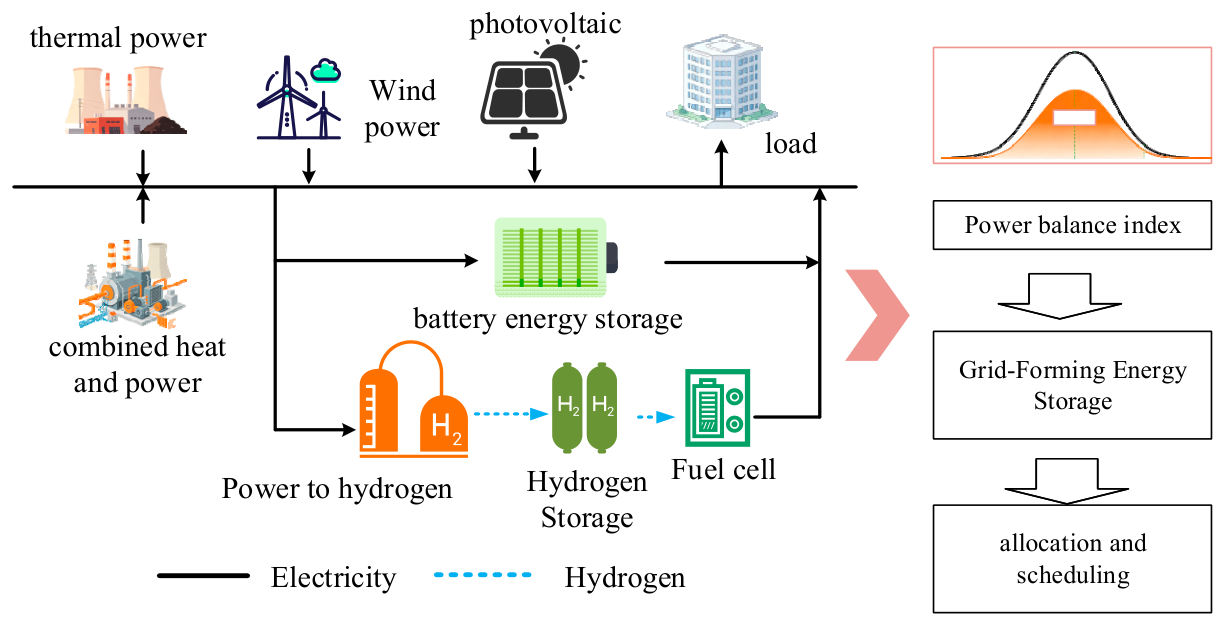
Figure 1 shows the overall structure of new power system GFM-EHS. The battery energy storage represents the existing short-term storage in the original system and is retained as a benchmark/fast power-balancing device. The GFM-EHS itself consists of the electrolyzer, hydrogen tank, and fuel cell, all connected through GFM converters. On the power supply side, the system integrates wind power generation and photovoltaic power generation, as well as conventional thermal power units and combined heat and power (CHP). On the load side, in addition to electric load, the electric hydrogen production load is also configured. The electric energy is converted into hydrogen through electrolytic cell. After being stored in a hydrogen storage tank, the hydrogen fuel cell reversely generates electricity and feeds back to the grid when needed, forming an ‘electric-hydrogen-electric’ bidirectional energy conversion closed-loop. This structure provides a complete physical carrier for the study of power and energy balance-conventional power sources; new energy sources bear basic power supply, while electro-hydrogen energy storage bears the dual tasks of cross-period power regulation and instantaneous power support. It is worth emphasizing that the electrolytic cell, fuel cell and power storage equipment are connected to the AC bus through the Grid-Forming converter, so that it can not only respond to the scheduling instruction for energy time shift to improve the power balance, but also actively adjust the power output according to the system frequency change rate, provide virtual inertia support and primary frequency modulation service for system, and directly participate in the real-time power balance. On this basis, based on this structure, this paper focuses on construction of power and energy balance index system considering the fluctuation characteristics of source–load sides, and studies the inertia response control strategy of GFM-EHS and the optimal configuration and scheduling method considering frequency security constraints, so as to realize the unified coordination of the three-dimensional balance goal of ‘power-power-inertia’.

In order to establish a new power and energy balance index system of power system considering source–load fluctuation characteristics, the power balance margin, peak regulation demand index, flexible resource gap rate, power balance deviation, power fluctuation rate and source–load power matching degree are taken as the power and energy balance indexes of new power system.

Based on systematic analysis of source–load coupling characteristic index, a new power balance index system reflecting the synergistic effect of bilateral fluctuations is further constructed. Based on coupling characteristics of wind power, photovoltaic and load [7], an evaluation system including power balance margin, power balance deviation and flexible resource matching degree is constructed.

(1)

Power balance margin

$$M_{\mathrm{p},\mathrm{s}}={\displaystyle \frac{P_{\mathrm{G},\max }+P_{\mathrm{W},t}+P_{\mathrm{V},t}-P_{L,t}}{P_{L,t}}}\times 100\%$$

(1)

where M_p,s is the power balance margin; P_G,max is maximum output of the conventional power source, P_W,t is wind power output, P_V,t is photovoltaic power output, and P_L,t denotes load demand. This indicator reflects power supply margin of the system after accounting for the combined wind and solar power outputs.

(2)

Peak-shaving demand index

$${\gamma }_{\mathrm{p}}={\displaystyle \frac{|(L_{\max }-L_{\min })-(P_{\mathrm{Vmax}}-P_{{\mathrm{T}}_{\mathrm{H}},\mathrm{Wmin}})|}{\max (L_{\max }-L_{\min },P_{\mathrm{Vmax}})}}$$

(2)

where $P_{{\mathrm{T}}_{\mathrm{H}},\mathrm{Wmin}}$ is minimum wind power output during peak load periods, and P_Vmax is maximum photovoltaic power output. L_max, L_min are the maximum and minimum load requirements. γ_p is peak-shaving demand index.

(3)

Flexibility Resource Shortage Rate

$${\xi }_{\mathrm{p}}={\displaystyle \frac{\max (0,L_t-P_{\mathrm{W},t}-P_{\mathrm{V},t}-G_{\min })}{L_t}}\times 100\%$$

(3)

where G_min denotes the minimum technical output of conventional power sources. This indicator reflects the flexibility resource shortage arising when wind power output is at its lowest levels and photovoltaic systems exhibit zero output during nighttime hours. L_t is load requirements. ξ_p is flexibility resource shortage rate.

(4)

Electricity balance deviation:

$${\delta }_e={\displaystyle \frac{|{\displaystyle \sum (P_{\mathrm{W},t}+P_{\mathrm{V},t})}-{\displaystyle \sum L_t}|}{{\displaystyle \sum L_t}}}\times 100\%$$

(4)

where δ_e is electricity balance deviation.

(5)

Power fluctuation coefficient

$${\kappa }_e={\displaystyle \frac{\max (E_d)-\min (E_d)}{\mathit{avg}(E_d)}}\times 100\%$$

(5)

where E_d denotes the daily power generation sequence. κ_e is power fluctuation coefficient.

(6)

Source–load power matching degree

$${\rho }_e=1-{\displaystyle \frac{{\displaystyle \sum |}(P_{\mathrm{W},t}+P_{\mathrm{V},t})-L_t|}{2{\displaystyle \sum L_t}}}\times 100\%$$

(6)

where ρ_e is source–load power matching degree.

Power, energy, and inertia describe complementary aspects of source–load imbalance. The power-related indicators in Equations (1)–(3) characterize the instantaneous supply margin and the demand placed on flexible resources. The energy-related indicators in Equations (4)–(6) describe renewable generation and load matching over the observation horizon, including accumulated mismatch and temporal variation. These matching indicators should be distinguished from the system-wide balance after dispatch of conventional generation and storage. Even when accumulated generation and demand are closely matched, individual periods can still require substantial upward or downward power regulation.

The inertia dimension concerns the initial frequency response following an active power disturbance. It is represented by the capacity-weighted synchronous and virtual inertia in Equations (20) and (21), with its adequacy assessed against the RoCoF and frequency deviation requirements in Equations (18) and (19). Sufficient installed power or stored energy alone does not determine whether this support can be delivered within the required response time. The available operating headroom and response capability of the electrolyzer and fuel cell therefore connect the power and energy assessment to the frequency security assessment.

Power-adequacy assessments identify capacity shortages, energy-matching assessments identify time-shifting requirements, and inertia-oriented assessments identify limitations in the initial disturbance response. The proposed framework considers these requirements together for electro-hydrogen storage. Its contribution lies in linking imbalance assessment, converter-mediated power support, and frequency-constrained configuration and dispatch, rather than treating any individual indicator as a substitute for all three functions. This connection distinguishes the long-duration energy-shifting role of hydrogen storage from the short-duration support available at a particular operating point and provides a consistent interpretation of the configuration and operating results.

3. Grid-Forming Electro-Hydrogen Energy Storage Inertia Response Control Strategy

3.1. Grid-Forming Electro-Hydrogen Energy Storage Power Support

The virtual inertia contribution is interpreted as a converter-mediated change in net power injection around the scheduled operating point. Positive support denotes an increase in power supplied to the AC system. Accordingly, a fuel cell supports a falling frequency by increasing generation, whereas an electrolyzer provides equivalent support by reducing its electrical consumption. The reverse actions apply when downward support is required. Only a connected device in an admissible operating state can provide this response; installed capacity alone does not imply that the full rated power is available for frequency support.

Equations (7) and (8) represent an ideal reduced-order response under the assumption that electrical power tracking is sufficiently fast relative to the frequency-response timescale considered. This assumption does not equate converter response with stack start-up or gas-supply dynamics. In practical operation, the delivered response is also affected by control and filtering delays, converter bandwidth, stack ramping capability, and auxiliary-process dynamics. The ideal relation is therefore applicable only while the requested response can be tracked within the required time and without activating device protection. An unavailable or shut-down stack is not treated as an instantaneous reserve merely because it has a nonzero nameplate rating.

The admissible response is determined by the scheduled operating point and the physical limits already represented in the model. During a frequency drop, the relevant power headroom is the difference between the fuel-cell maximum output and its scheduled output, and the difference between the scheduled electrolyzer consumption and its minimum admissible consumption. These margins reverse for the opposite support direction. Equations (10) and (11) bound the directional reserve, while Equations (32)–(38) describe current, ramping, hydrogen-inventory, and operating-state restrictions. Inertial support and primary frequency response draw on the same device capability; their combined request must remain within the available headroom and ramping limits. These conditions define the physical validity range of the simplified virtual inertia response.

Fuel cells and electrolyzer stacks are connected to power grid via power electronic converters and are equipped with virtual synchronous generator control. The fuel cells and electrolyzers adjust their output or input power based on the frequency change rate to provide virtual inertia support. During the virtual inertia response phase, the fuel cells and electrolyzers rapidly adjust their operating power to provide inertia response support [2].

The fuel cell virtual inertia response-supported power $\Delta P_{F,t}^{\mathrm{VI}}$ and the electrolyzer virtual inertia response-supported power $\Delta P_{E,t}^{\mathrm{VI}}$ can be expressed as follows:

$$\Delta P_{F,t}^{\mathrm{VI}}=-2H_F{\displaystyle \frac{d\Delta f(t)}{\mathit{dt}}}{\displaystyle \frac{P_F^{\max }}{f_0}}$$

(7)

$$\Delta P_{E,t}^{\mathrm{VI}}=-2H_E{\displaystyle \frac{d\Delta f(t)}{\mathit{dt}}}{\displaystyle \frac{P_E^{\max }}{f_0}}$$

(8)

where H_F and H_E are virtual inertia time constants of fuel cell stack F and the electrolyzer stack E; $P_F^{\max }$ and $P_E^{\max }$ denote maximum operating power of fuel cell stack F and electrolyzer stack E, respectively; f₀ is the rated frequency, with a value of 50 Hz; and Δf(t) denotes the system frequency deviation during period t.

Considering virtual inertia and frequency support of fuel cells and electrolyzers, the dynamic frequency model for the new power system is

$${\displaystyle \frac{2\left[H_{\mathrm{G}}+\left(H_{\mathrm{E}}^{\mathrm{VI}}+H_{\mathrm{F}}^{\mathrm{VI}}\right)\right]}{f_0}}{\displaystyle \frac{\mathrm{d}\Delta f\left(t\right)}{\mathrm{d}t}}+D\Delta f\left(t\right)={\displaystyle \sum _{E=1}^{N_{\mathrm{E}}}}\Delta P_{E,t}^{\mathrm{PFR}}+{\displaystyle \sum _{F=1}^{N_{\mathrm{F}}}}\Delta P_{F,t}^{\mathrm{PFR}}+{\displaystyle \sum _{g=1}^{N_G}}\Delta P_{g,t}^{\mathrm{PFR}}-\Delta P_{\mathrm{L}}$$

(9)

where N_G denotes number of thermal power units; H_G denotes synchronous inertia; $\Delta P_{E,t}^{\mathrm{PFR}}$, $\Delta P_{F,t}^{\mathrm{PFR}}$, $\Delta P_{g,t}^{\mathrm{PFR}}$ denote the primary frequency regulation power outputs of electrolyzer stack E, fuel cell stack F, and thermal power unit g, respectively; ΔP_L denotes the system’s unbalanced power; and D denotes load damping coefficient of the power system, with units of MW/Hz.

If the system frequency increases, then Δf(t) > 0, causing the electrolyzer to increase its operating power while thermal power generation unit and fuel cell reduce their power output, thereby supporting the system in lowering its frequency [13]; under such conditions, the frequency regulation power change limits for thermal power generation unit, fuel cell, and electrolyzer should be set to smaller than the rapid power variation limit and downward frequency regulation power change limit.

$$\left\{\begin{array}{l}\left|\Delta P_{g,t}^{\mathrm{PFR}}\right|\le \min \left\{R_g^{\mathrm{r}},R_g^{\max }{u}_{g,t}\right\}\\ \left|\Delta P_{F,t}^{\mathrm{PFR}}\right|\le \min \left\{R_F^{\mathrm{r}},(P_F^{\max }-P_{F,t})u_{F,t}\right\}\\ \left|\Delta P_{E,t}^{\mathrm{PFR}}\right|\le \min \left\{R_E^{\mathrm{r}},(P_{E,t}-P_E^{\min })u_{E,t}\right\}\end{array}\right.$$

(10)

$$\left\{\begin{array}{l}\left|\Delta P_{g,t}^{\mathrm{PFR}}\right|\le \min \left\{R_g^{\mathrm{r}},R_g^{\max }{u}_{g,t}\right\}\\ \left|\Delta P_{F,t}^{\mathrm{PFR}}\right|\le \min \left\{R_F^{\mathrm{r}},(P_{F,t}-P_F^{\min })u_{F,t}\right\}\\ \left|\Delta P_{E,t}^{\mathrm{PFR}}\right|\le \min \left\{R_E^{\mathrm{r}},(P_E^{\max }-P_{E,t})u_{E,t}\right\}\end{array}\right.$$

(11)

where $R_g^{\max }$ represents maximum primary frequency regulation reserve capacity of thermal power unit g; $P_F^{\max }$ represents minimum operating power of fuel cell stack F; $P_E^{\min }$ represents minimum operating power of electrolysis cell stack E; $R_g^{\mathrm{r}}$ represents the primary frequency regulation power variation limit for thermal power unit g; $R_F^{\mathrm{r}}$ represents the rapid power variation limit for fuel cell stack F; $R_E^{\mathrm{r}}$ represents the rapid power variation limit for electrolysis cell stack E; and u_g,t represents the operating status variable of thermal power unit g during time interval, where the value is 1 when the unit is in operation and 0 when the unit is shut down.

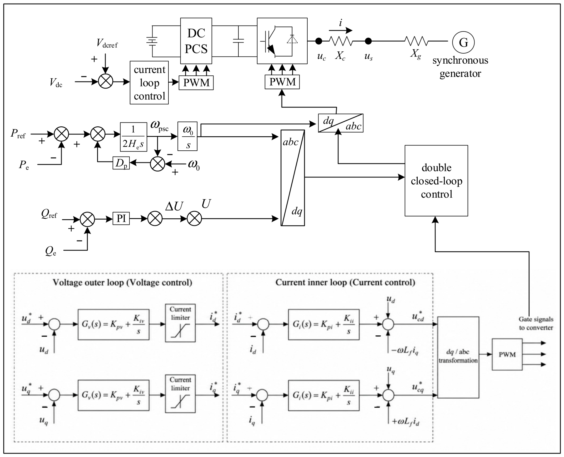
The control block diagram for Grid-Forming control and a comparison of its inertia response process are shown in Figure 2.

The upper path is the DC-link voltage control loop: V_dcref is compared with V_dc, and the error is passed to a current-loop controller and PWM modulator. The lower path is the VSG-based AC control: P_ref and P_e generate the active power error, which is fed into the swing equation P_ref − P_e − D_cΔω_pc to obtain Δω_pc,ω, and the phase angle θ. Q_ref and Q_e generate the reactive power error, which is passed through a PI controller to obtain the voltage magnitude E. The double closed-loop control consists of an outer power/voltage loop and an inner current loop. The inner current loop regulates i_d and i_q and outputs u_d and u_q. The abc/dq transformation and PWM modulator generate the converter switching signals.

The GFM converter is controlled through a hierarchical structure consisting of an outer virtual–synchronous machine layer and an inner cascaded voltage–current control layer. In the active power/frequency loop, the difference between the active power reference P_ref and measured active power P is processed by the virtual swing equation to generate the converter angular-frequency reference. The “double closed-loop control” block in the original figure is expanded into an outer capacitor-voltage loop and an inner converter-current loop. The voltage controller generates the dq-axis current references i_d* and i_q*, while the current controller generates the converter voltage references u_d* and u_q*. These voltage commands are transformed from the dq frame to the abc frame and supplied to the PWM modulator. This cascaded structure allows the converter to track the VSM-generated voltage and frequency references while maintaining fast current regulation during inertial and primary-frequency-response processes.

Virtual synchronous of GFM-EHS control is shown in the following equation:

$$2H_{\mathrm{e}}{\displaystyle \frac{\mathrm{d}\Delta {\omega }_{\mathrm{psc}}}{\mathrm{d}t}}=P_{\mathrm{ref}}-P_{\mathrm{e}}-D_{\mathrm{e}}\Delta {\omega }_{\mathrm{psc}}$$

(12)

where H_e and D_e represent virtual inertia and electrical damping, respectively; P_ref is energy storage power reference value; and Δω_psc is frequency deviation.

3.2. Virtual Inertia Response Model for GFM-EHS Stack

Fuel cells and electrolyzer stacks are connected to power grid via power electronic converters and are equipped with virtual synchronous generator control. Grid-Forming hydrogen energy storage systems adjust their output or input power based on the RoCoF, thereby providing virtual inertia support.

According to the unified source/load sign convention defined in Section 3.1, the virtual inertia power responses of the fuel-cell and electrolyzer stacks are directly given by Equations (7) and (8), respectively. These equations are therefore not repeated here.

The virtual inertia time constants of the electrolyzer and fuel cell are controller gains, rather than mechanical inertia constants inherent to the stacks. Their selection must be consistent with the power rating, scheduled operating point, admissible current, and response dynamics of each converter–stack combination. The device-level time constants and the capacity-weighted system inertia used in the frequency constraints must also be expressed on consistent power and frequency bases.

A necessary power-feasibility condition follows directly from Equations (7) and (8). For a design RoCoF magnitude and an available directional power margin, the candidate gain must satisfy

$$0\le H_i\le {\displaystyle \frac{f_0\cdot \Delta P_{i,t}^{\mathit{avail}}}{2P_i^{\mathit{max}}{r}_{\mathit{max}}}},\hspace{1em}i\in \{E,F\}$$

(13)

Here, the design RoCoF magnitude is denoted by r_max, and the available power margin is the part of the directional operating headroom that remains available for inertial support after accounting for simultaneous service requirements and physical limits. The margin is operating-point dependent and may differ between upward and downward support. If this margin is zero, a positive virtual inertia gain does not create deliverable inertial power in that direction. Equation (13) is a necessary power bound, not a sufficient condition for closed-loop stability.

The converter current limit provides a further restriction because active power support and reactive power provision share the same current capability. DC-side energy availability and stack dynamics must sustain the commanded power for the response interval. Increasing the inertia gain increases the required power excursion for a prescribed RoCoF and can therefore cause saturation even if the ideal frequency model predicts improved RoCoF suppression. The inertia and damping gains should consequently be selected jointly within the admissible power envelope and checked against response delay, settling behavior, and current limitation. The ideal model is applicable to operating points for which these tracking and headroom conditions remain satisfied.

4. Optimal Configuration and Dispatch Method for Grid-Forming Electro-Hydrogen Energy Storage Systems Incorporating Inertia Support

4.1. Grid-Forming Electro-Hydrogen Energy Storage Optimization Model

The proposed combined operation model for conventional power units and energy storage systems aims to minimize total cost of power generation, peak shaving, and frequency regulation, with objective function defined by the following equation for optimal dispatch solution.

$$\begin{array}{c}F=\min \left\{{\displaystyle \sum _{i=1}^4}{\displaystyle \sum _{j=1}^6}{\displaystyle \sum _{t=1}^{24}}\left[{\rho }_{\mathit{ij}}{\displaystyle \sum _{m=1}^{N_G}}(C_{\mathit{ij},m,t}^{\mathrm{G},\mathrm{op}}+C_{\mathit{ij},m,t}^{\mathrm{G},\mathrm{pr}}+C_{\mathit{ij},m,t}^{\mathrm{G},\mathrm{ss}}+C_{\mathit{ij},m,t}^{\mathrm{G},\mathrm{re}})+C_{\mathit{ij},t}^{\mathrm{E},\mathrm{pr}}+C_{\mathit{ij},t}^{\mathrm{E},\mathrm{re}}+C_{\mathit{ij},t}^{\mathrm{WVL}}\right]\right\}\end{array}$$

(14)

where the subscript ij denotes the corresponding variable under the peak shaving typical day i and frequency regulation typical scenario j; $C_{\mathit{ij},m,t}^{\mathrm{G},\mathrm{op}}$, $C_{\mathit{ij},m,t}^{\mathrm{G},\mathrm{pr}}$, $C_{\mathit{ij},m,t}^{\mathrm{G},\mathrm{ss}}$, and $C_{\mathit{ij},m,t}^{\mathrm{G},\mathrm{re}}$ represent the operating, peak-shaving, start/stop, and standby cost functions of conventional units during time slot. $C_{\mathit{ij},t}^{\mathrm{E},\mathrm{pr}}$ and $C_{\mathit{ij},t}^{\mathrm{E},\mathrm{re}}$ represent the peak-shaving and frequency-regulation standby cost functions of energy storage systems during time slot; $C_{\mathit{ij},t}^{\mathrm{WVL}}$ represents the penalty function for new energy generation and load curtailment during time slot. N_G represents the total number of conventional units. ρ_ij is correction factor. F is objective function for optimal dispatch solution.

$$\left\{\begin{array}{l}{C}_{\mathit{ij},m,t}^{\mathrm{G},\mathrm{op}}=a_m{\left(p_{\mathit{ij},m,t}^{\mathrm{G}}\right)}^2+b_m{p}_{\mathit{ij},m,t}^{\mathrm{G}}+c_m{x}_{\mathit{ij},m,t}^{\mathrm{G}}\hfill \\ C_{\mathit{ij},m,t}^{\mathrm{G},\mathrm{pr}}=u_{\mathit{ij},m,t}^{\mathrm{G}1}{d}_{1,t}\left(p_{m,\max }^{\mathrm{G}}-p_{\mathit{ij},m,t}^{\mathrm{G}}\right)+u_{\mathit{ij},m,t}^{\mathrm{G}2}{d}_{2,t}\left(p_{m,\mathrm{mid}}^{\mathrm{G}}-p_{\mathit{ij},m,t}^{\mathrm{G}}\right)\hfill \\ C_{\mathit{ij},m,t}^{\mathrm{G},\mathrm{ss}}=C_{\mathit{ij},m,t}^{\mathrm{G},\mathrm{start}}+C_{\mathit{ij},m,t}^{\mathrm{G},\mathrm{stop}}\hfill \\ C_{\mathit{ij},m,t}^{\mathrm{G},\mathrm{re}}={\displaystyle \sum _{k\in {\Lambda }_t}\left(e_{\mathrm{up},m}{r}_{\mathit{ij},m,t,k}^{\mathrm{G},\mathrm{up}}+e_{\mathrm{down},m}{r}_{\mathit{ij},m,t,k}^{\mathrm{G},\mathrm{down}}\right)}\hfill \\ C_{\mathit{ij},t}^{\mathrm{E},\mathrm{pr}}=z_{\mathrm{up}}{p}_{\mathit{ij},t}^{\mathrm{E},\mathrm{pr},\mathrm{up}}+z_{\mathrm{down}}{p}_{\mathit{ij},t}^{\mathrm{E},\mathrm{pr},\mathrm{down}}\hfill \\ C_{\mathit{ij},t}^{\mathrm{E},\mathrm{re}}={\displaystyle \sum _{k\in {\Lambda }_t}\left(k_{\mathrm{up}}{r}_{\mathit{ij},t,k}^{\mathrm{E},\mathrm{re},\mathrm{up}}+k_{\mathrm{down}}{r}_{\mathit{ij},t,k}^{\mathrm{E},\mathrm{re},\mathrm{down}}\right)}\hfill \\ C_{\mathit{ij},t}^{\mathrm{WVL}}=k_1{P}_{\mathit{ij},t}^{\mathrm{W}}+k_2{P}_{\mathit{ij},t}^{\mathrm{V}}+k_3{P}_{\mathit{ij},t}^{\mathrm{L}}\hfill \end{array}\right.$$

(15)

where a_m, b_m, c_m represent the power generation cost coefficients for conventional generating units; $p_{\mathit{ij},m,t}^{\mathrm{G}}$ denotes active power output of conventional generating units during period t; $x_{\mathit{ij},m,t}^{\mathrm{G}}$ indicates start/stop status of conventional generating units during period t; d_1,t and d_2,t are cost coefficients corresponding to different peak shaving depths; $p_{m,\mathrm{mid}}^{\mathrm{G}}$ and $p_{m,\max }^{\mathrm{G}}$ represent minimum peak shaving boundary and rated power of conventional generating units, respectively; $u_{\mathit{ij},m,t}^{\mathrm{G}1}$ and $u_{\mathit{ij},m,t}^{\mathrm{G}2}$ is the peak shaving depth characterization value for conventional generating units during period t. $p_{m,\min }^{\mathrm{G}}$ is the minimum active power for conventional units. $C_{\mathit{ij},m,t}^{\mathrm{G},\mathrm{start}}$ and $C_{\mathit{ij},m,t}^{\mathrm{G},\mathrm{stop}}$ are costs associated with start-up and shutdown of conventional power units for respective time periods. k is frequency regulation time series identifier for peak-shaving periods. Λ_t is a set of frequency modulation time series for peak-shaving periods. $r_{\mathit{ij},m,t,k}^{\mathrm{G},\mathrm{up}}$ and $r_{\mathit{ij},m,t,k}^{\mathrm{G},\mathrm{down}}$ represent upper and lower reserve capacities of the conventional unit m. e_up,m and e_down,m represent upper and lower standby cost coefficients for conventional power unit m, respectively. $p_{\mathit{ij},t}^{\mathrm{E},\mathrm{pr},\mathrm{up}}$ and $p_{\mathit{ij},t}^{\mathrm{E},\mathrm{pr},\mathrm{down}}$ represent the peak reserve power for electric–hydrogen energy storage during the respective time period. z_up and z_down represent upper and lower peak cost coefficients for electrical and hydrogen energy storage, respectively. $r_{\mathit{ij},t,k}^{\mathrm{E},\mathrm{re},\mathrm{up}}$ and $r_{\mathit{ij},t,k}^{\mathrm{E},\mathrm{re},\mathrm{down}}$ represent the upper and lower frequency reserve powers for time-specific electricity–hydrogen energy storage systems, respectively. k_up and k_down represent the upper and lower frequency adjustment cost coefficients for electrical and hydrogen energy storage systems, respectively. k₁, k₂, k₃ represent the curtailment cost coefficients for wind, solar, and load, respectively; $P_{\mathit{ij},t}^{\mathrm{W}}$, $P_{\mathit{ij},t}^{\mathrm{V}}$, $P_{\mathit{ij},t}^{\mathrm{L}}$ represent the curtailed power for wind, solar, and load during respective time periods.

During the configuration capacity optimization phase for electrical–hydrogen energy storage systems, an objective function is defined based on initial investment cost of GFM-EHS.

$$f_2=F+{\displaystyle \frac{\min \left((K_{\mathrm{P}}{P}_{\mathrm{e}}+K_{\mathrm{E}}{E}_{\mathrm{e}})\frac{r{(1+r)}^n}{{(1+r)}^n-1}\right)}{365}}$$

(16)

where K_P and K_E represent unit cost of electrical and hydrogen energy storage power capacity and energy capacity of GFM-EHS; r is benchmark discount rate; and n denotes operational lifespan of electrical and hydrogen energy storage system of GFM-EHS. f₂ is initial investment cost.

4.2. Frequency Security Constraints for Power Systems Considering Hydrogen-Based Virtual Inertia

(1)

Maximum RoCoF constraint

To prevent excessive instantaneous fluctuations in system frequency caused by unbalanced active power disturbances, a maximum RoCoF and $f_{\mathrm{RoCoF}}^{\max }$ is set to increase system inertia [15] and limit rate of change in system frequency f_RoCoF, as shown in the following equation.

$$\left|f_{\mathrm{RoCoF}}\right|=\left|{\displaystyle \frac{-\Delta P_{\mathrm{L}}{f}_0}{2(H_{\mathrm{G}}+H_{\mathrm{E}}^{\mathrm{VI}}+H_{\mathrm{F}}^{\mathrm{VI}})}}\right|\le f_{\mathrm{RoCoF}}^{\max }$$

(17)

During the inertia response phase, RoCoF is directly proportional to power imbalance magnitude and inversely proportional to the system inertia. Under identical power disturbances, a larger system inertia results in a lower RoCoF. By incorporating the virtual inertia support capability of fuel cells and electrolyzers, RoCoF can be effectively reduced, thereby enhancing resilience to frequency fluctuations.

(2)

Maximum Frequency Deviation Constraint

Under an unbalanced active power disturbance, when disruption event occurrence time t_r is not less than time t_DB when the frequency deviation reaches the frequency regulation dead zone, i.e., t_r ≥ t_DB, Δf(t)≥Δf_DB, the electrolyzer, fuel cell, and thermal power unit all participate in primary frequency regulation. When frequency reaches its minimum value (during t∗ interval), the frequency deviation shall not exceed the specified threshold Δf_max; the maximum system frequency deviation constraint is:

$$\left|\Delta f(t^{\ast })\right|=\left|{\displaystyle \frac{-2H{P}_{\mathrm{g}}^{\mathrm{tot}}}{D^2{f}_0{T}_{\mathrm{g}}}}\ln \left(H{P}_{\mathrm{g}}^{\mathrm{tot}}\right)+{\displaystyle \frac{P_{\mathrm{E}}^{\mathrm{tot}}+P_{\mathrm{F}}^{\mathrm{tot}}-\Delta P_{\mathrm{L}}}{D}}\right|\le \Delta f_{\max }$$

(18)

$$H=H_{\mathrm{G}}+H_{\mathrm{E}}^{\mathrm{VI}}+H_{\mathrm{F}}^{\mathrm{VI}}$$

(19)

$$H_{\mathrm{G}}={\displaystyle \sum _{g=1}^{N_{\mathrm{G}}}}{P}_g^{\max }{H}_g{u}_{g,t}$$

(20)

where H represents total inertia of the new power system; $P_{\mathrm{E}}^{\mathrm{tot}}, P_{\mathrm{F}}^{\mathrm{tot}}, P_{\mathrm{g}}^{\mathrm{tot}}$ denote total frequency regulation power outputs of electrolytic cell, fuel cell, and thermal power unit, respectively; $P_g^{\max }, H_g$ represent rated power and inertia time constant of thermal power unit g, respectively; T_g denotes primary frequency regulation response time of thermal power unit.

Under identical unbalanced power disturbances, the higher the primary frequency regulation power of fuel cell or electrolyzer, the smaller the maximum frequency deviation. Thanks to the virtual inertia support provided by electrolyzer and fuel cell, the highly nonlinear function governing the maximum frequency deviation highlights frequency regulation potential of both electrolyzer and the fuel cell. To address this, an effective linearization method [6] is proposed, enabling the incorporation of this constraint into a mixed-integer nonlinear programming problem.

$$D^2{f}_0{T}_{\mathrm{g}}{\displaystyle \frac{P_{\mathrm{E}}^{\mathrm{tot}}+P_{\mathrm{F}}^{\mathrm{tot}}-\Delta P_{\mathrm{L}}}{D}}\le D^2{f}_0{T}_{\mathrm{g}}\Delta f_{\max }+2H{P}_{\mathrm{g}}^{\mathrm{tot}}\ln \left(H{P}_{\mathrm{g}}^{\mathrm{tot}}\right)$$

(21)

The nonlinear term on the right-hand side of Equation (21) is treated by a finite tangent approximation, while products of binary operating-state variables and bounded continuous variables are represented using the Big-M formulation. The resulting MILP is a tractable approximation of the nonlinear formulation. Its solver optimality certificate applies to the approximating MILP; the feasibility and accuracy of the obtained solution with respect to the original nonlinear frequency relation require a separate evaluation.

$$D^2{f}_0{T}_{\mathrm{g}}{\displaystyle \frac{P_{\mathrm{E}}^{\mathrm{tot}}+P_{\mathrm{F}}^{\mathrm{tot}}-\Delta P_{\mathrm{L}}}{D}}\le D^2{f}_0{T}_{\mathrm{g}}\Delta f_{\max }+g_v(x)$$

(22)

$$\begin{array}{c}{g}_v\left(x\right)=\nabla g_v\left({\widehat{x}}^{(k)}\right)(x-{\widehat{x}}^{(k)})+g_v\left({\widehat{x}}^{(k)}\right)v\in \{1,2,\cdots ,m\},{\widehat{x}}^{(k)}\in \chi \end{array}$$

(23)

$$x={\displaystyle \sum _{g=1}^{N_{\mathrm{G}}}}{P}_g^{\max }{H}_g{y}_1+{\displaystyle \sum _{E=1}^{N_{\mathrm{E}}}}{P}_E^{\max }{H}_E{y}_2+{\displaystyle \sum _{F=1}^{N_{\mathrm{F}}}}{P}_F^{\max }{H}_F{y}_3$$

(24)

$$-M\left(1-u_{g,t}\right)\le y_1-P_g^{\mathrm{tot}}\le M\left(1-u_{g,t}\right)$$

(25)

$$-M{u}_{g,t}\le y_1\le M{u}_{g,t}$$

(26)

$$-M(1-u_{E,t})\le y_2-P_{\mathrm{g}}^{\mathrm{tot}}\le M(1-u_{E,t})$$

(27)

$$-M{u}_{E,t}\le y_2\le M{u}_{E,t}$$

(28)

$$-M(1-u_{F,t})\le y_3-P_g^{\mathrm{tot}}\le M(1-u_{F,t})$$

(29)

−Mu_F,t ≤ y₃ ≤ Mu_F,t

(30)

where $y_1=u_{g,t}{P}_{\mathrm{g}}^{\mathrm{tot}}; y_2=u_{E,t}{P}_{\mathrm{g}}^{\mathrm{tot}}; y_3=u_{F,t}{P}_{\mathrm{g}}^{\mathrm{tot}}; g_v(x)$ denotes the tangent approximation function. $\chi =\{{\widehat{x}}^{(1)},{\widehat{x}}^{(2)},\cdots ,{\widehat{x}}^{(K)}\}$ is the set of sample points. K denotes the number of sample points when using virtual inertia support. $g_v({\widehat{x}}^{(k)})(k=1,2,\cdots ,K;v=1,2,\cdots ,m)$ is the function value at the sample point ${\widehat{x}}^{(k)}$. m denotes the quantity of $g_v\left(x\right)$. $\nabla g_v({\widehat{x}}^{(k)})$ is the slope at the sample point. M is the parameters for the Big M method.

The nonlinear frequency deviation constraint is linearized by the convex-function outer-approximation tangent method. In the revised model, K = 10 tangent sample points are adaptively selected over the feasible inertia interval H∈[0.8H_min,1.2H_max]. The convergence and tightness were verified by increasing K from 5 to 20. when K = 10, the relative gap of the objective function is only 0.11%, the maximum constraint violation is below 8 × 10⁻⁴ Hz, and the maximum RoCoF error is below 0.001 Hz/s. Further increasing K to 15 and 20 changes the objective by less than 0.04% and 0.00%, respectively, while the computation time increases significantly. Therefore, K = 10 is adopted as a good trade-off between accuracy and computational efficiency.

For a convex scalar function g on the positive domain of the approximation variable x, the tangent at a sample point provides a lower bound:

ℓ_k(x) = g(x_k) + g^′(x_k)(x − x_k) ≤ g(x)

(31)

For the scalar term g(x) = 2x ln(x), its second derivative is 2/x > 0. On a bounded interval with a positive lower bound x_min, the local tangent error satisfies

$$0\le g(x)-{\mathcal{l}}_k(x)\le {\displaystyle \frac{{(x-x_k)}^2}{x_{\mathit{min}}}}$$

(32)

Thus, the error depends on both the spacing of the sample points and the curvature over the sampled domain. The inertia range must be interpreted together with the admissible range of the total conventional frequency-response power when determining the range of x in Equation (26). A sampling interval for inertia alone does not specify the full domain of their product. The positive-domain requirement must also be respected when constructing the sample points. Since the nonlinear term appears on the right-hand side of Equation (23), substitution by a lower tangent yields a sufficient, potentially conservative condition for that rewritten inequality. This scalar bound does not establish that the complete nonlinear frequency formulation is exactly represented by a finite number of tangents.

For the binary–continuous products in Equations (27)–(32), let the continuous total frequency-response power be bounded by L_P and U_P. A valid bound-based choice for the common Big-M coefficient is

$$M\ge \max \left\{\right|L_P|,|U_P\left|\right\},L_P\le P_g^{\mathit{tot}}\le U_P$$

(33)

When the operating-state variable is zero, the auxiliary variable is forced to zero; when it is one, the auxiliary variable equals the original continuous variable. The remaining inequalities must be inactive over the entire admissible continuous-variable range. This explains why M is derived from physical reserve bounds rather than selected as an arbitrary large constant. In exact arithmetic, this binary–continuous reformulation is exact when valid bounds are used. Numerical feasibility and integrality tolerances still affect the implemented solution, and an unnecessarily large M can weaken the relaxation and magnify numerical difficulties.

Approximation accuracy and solver convergence describe different quantities. The objective discrepancy measures the effect of the approximation relative to its stated reference, whereas the MILP optimality gap measures the separation between the incumbent objective and the solver bound for the approximating model. Frequency accuracy is evaluated by substituting the obtained operating decisions into the original nonlinear relation and checking the resulting frequency deviation against its limit. The existing comparison over different K values provides numerical evidence for the tested cases, but does not constitute a general proof of zero approximation error or global optimality of the original nonlinear problem.

(3)

Electrical and Hydrogen Energy Storage Equipment Constraints

To prevent structural damage to the electrolytic cell caused by current surges, the current density i_e,t should satisfy the following requirement:

$$i_e^{\min }\le i_{e,t}\le i_e^{\max }$$

(34)

where $i_e^{\max }, i_e^{\min }$ represent upper and lower limits of the input current density into the electrolytic cell e.

The fuel cell micro-element current I_f,t must satisfy the following condition:

$$I_f^{\min }\le I_{f,t}\le I_f^{\max }$$

(35)

where $I_f^{\max }, I_f^{\min }$ represent the upper and lower limits of the output current for the fuel cell element f.

To prevent accelerated life degradation due to rapid power regulation, the operating power of fuel cells and electrolyzers shall comply with the rapid power regulation support constraint, as shown below.

$$-R_F^{\mathrm{dn}}\le P_{F,t}-P_{F,t-1}\le R_F^{\mathrm{up}}$$

(36)

$$-R_E^{\mathrm{dn}}\le P_{E,t}-P_{E,t-1}\le R_E^{\mathrm{up}}$$

(37)

where $R_F^{\mathrm{up}}, R_F^{\mathrm{dn}}$ represent upward and downward ramp power limits, respectively, for the fuel cell stack F; $R_E^{\mathrm{up}},R_E^{\mathrm{dn}}$ represent the upward and downward ramp power limits, respectively, for the electrolysis stack E.

The hydrogen storage capacity of the hydrogen storage tank meets the requirements.

$$S_i^{\min }\le S_{i,t}\le S_i^{\max }\hspace{1em}i\in N_{\mathrm{b}}$$

(38)

S_i,t = S_i,t−1 + (η_cP_E,t − P_F,t/η_d)Δt

(39)

where S_i,t denotes hydrogen storage capacity of hydrogen storage tank at busbar i during time interval t, with units of MW·h; $S_i^{\min },S_i^{\max }$ represent minimum and maximum storage capacities of the hydrogen storage tank at busbar i, respectively; N_b denotes the set of all busbars; η_c is electrochemical hydrogen-to-hydrogen conversion efficiency of the electrolyzer; η_d is hydrogen-to-electricity conversion efficiency; Δt is unit time interval.

The operating conditions of the electrolytic cell and the fuel cell must be met.

u_E,t,b + u_F,t,b ≤ 1

(40)

where u_E,t,b and u_F,t,b represent operating status of the electrolysis stack E and the fuel cell stack F at busbar b during time interval t; when the stack is in production or standby mode, the value is 1; when the stack is shut down, the value is 0.

The maximum frequency deviation constraint involves complex nonlinear terms arising from product of continuous variables as well as product of continuous variables and binary variables; this results in the proposed optimization scheduling model with the maximum frequency deviation constraint being a mixed-integer nonlinear programming problem, which cannot be solved directly using commercial solvers. To facilitate the solution of this model, the convex-function outer-approximation tangent method and the large-M method are employed to linearize the maximum frequency deviation constraint, thereby transforming mixed-integer nonlinear programming problem into a mixed-integer linear programming problem, which is solved using the Gurobi/CPLEX commercial solver.

5. Case Study

5.1. Configuration Simulation Example for Grid-Forming Electro-Hydrogen Energy Storage System

This study simulates wind and solar power output based on actual data from a wind farm and a photovoltaic power station located in a certain province in Northwest China; the installed capacity of conventional thermal power unit is 200 MW; the system diagram is provided in Reference [7]. The case study is carried out on a modified 9-bus AC system with a 110 kV network and a 50 Hz rated frequency. The system integrates a 200 MW thermal power unit, an 80 MW CHP unit, a 200 MW wind farm, a 150 MW PV station, a 100 MW/200 MWh battery energy storage system, and a GFM-EHS consisting of an electrolyzer, a hydrogen tank, and a fuel cell. The peak load is 650 MW and the minimum load is 420 MW. All hydrogen and battery devices are connected to the AC bus through GFM converters. A system model was developed using MATLAB 2024a for simulation; the following comparative scenarios were configured.

The three scenarios in this subsection compare storage configuration choices. Scenario 1 is the baseline without additional GFM-EHS installation; the existing battery storage is retained, while the additional GFM-storage, electrolyzer, and fuel-cell capacities are zero, as reported in

Table 1. Energy Storage Configuration Optimization Results.

	Scenario 1	Scenario 2	Scenario 3
Grid-Forming energy storage power capacity/MW	0	208	113
Network energy storage capacity/(MW·h)	0	464	284
Electrolytic cell capacity/MW	0	212	231
Fuel cell capacity/MW	0	167	172
Battery power capacity (MW)	100	100	100
Battery energy capacity (MWh)	200	200	200
Energy storage peak frequency modulation cost/(104 yuan)	0	25.9	25.1
Initial construction cost of energy storage/104 yuan)	0	12.4	7.5
System equivalent daily cost/(104 yuan)	1415.9	759.9	585.8

. Scenario 2 introduces GFM-EHS and its frequency support capability, but excludes initial construction and equipment-degradation costs from the configuration objective. Scenario 3 uses the same frequency support and frequency security formulation as Scenario 2 and includes both initial construction and equipment-degradation costs in the configuration objective. The renewable generation and load profiles, existing equipment, and technical parameter assumptions are held consistent for this configuration comparison.

The comparison between Scenarios 2 and 3 therefore concerns the joint influence of construction and degradation costs on configuration decisions. It does not separately identify their individual effects, because both terms are changed together. Excluding a cost from the optimization objective does not imply that the equipment has no physical construction cost or undergoes no degradation; this distinction also explains why a construction-cost component can still be reported for a configuration obtained without that term in its objective. Scenario 1 provides a reference with a different equipment portfolio, rather than a controlled ablation of the frequency security constraint alone. The separate effects of frequency security requirements and hydrogen-based frequency support are examined through the dispatch scenarios in Section 5.2.

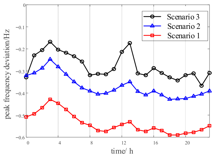
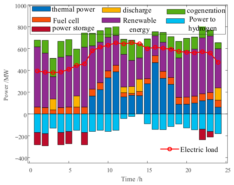
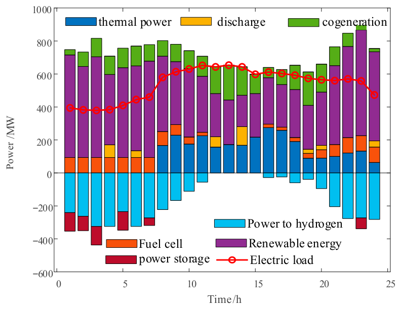
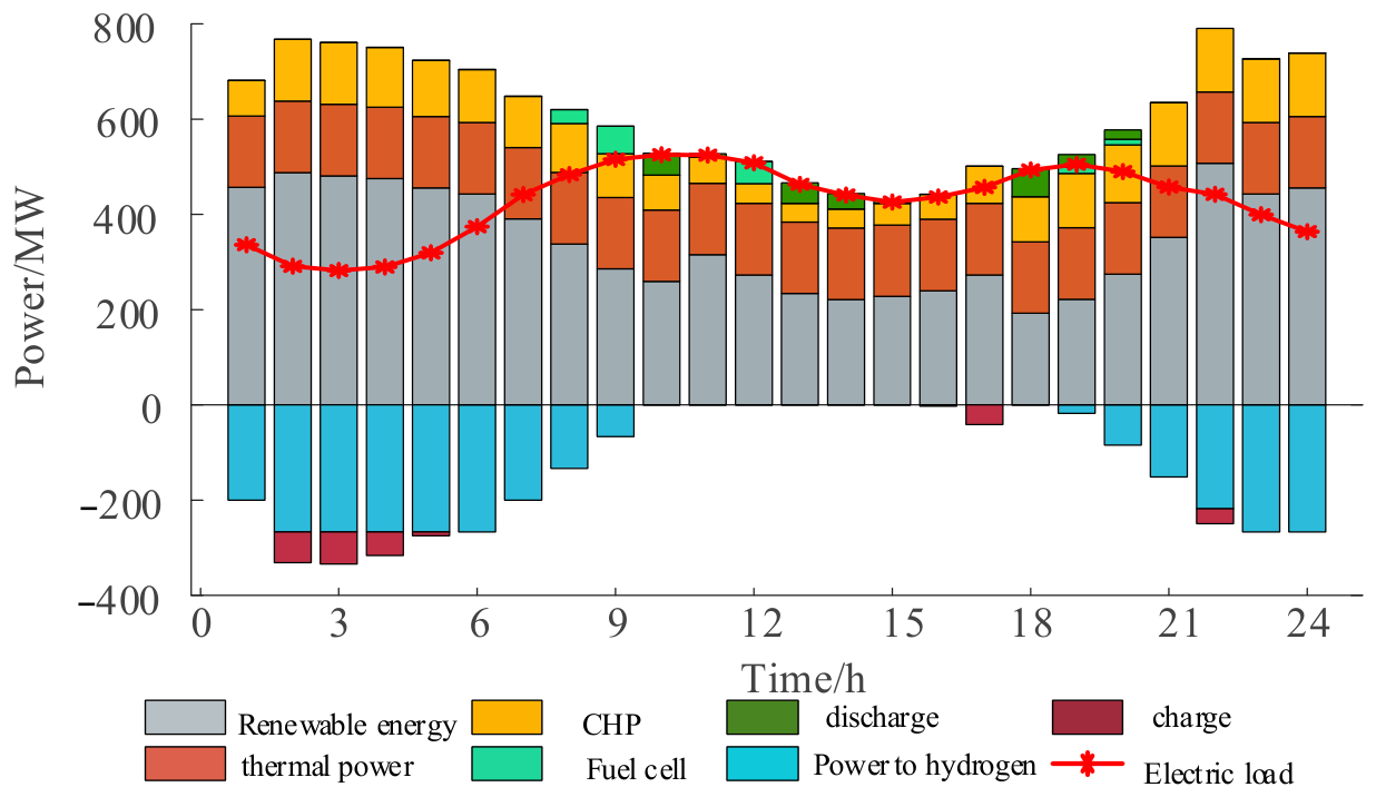
As can be seen from Figure 3, compared to Scenario 1 and Scenario 2, Scenario 3 exhibits a significant reduction in frequency deviation, indicating that considering Grid-Forming electric hydrogen energy storage can effectively reduce system frequency offset. By comparing Figure 4, Figure 5 and Figure 6, it is evident that in Scenario 1, due to the lack of consideration for optimal capacity allocation of Grid-Forming electric hydrogen energy storage, the system primarily relies on existing electricity storage devices to enhance the wind and solar power absorption rate. However, due to the capacity limitations of these electricity storage devices, the system cannot fully absorb wind and solar power, resulting in curtailment of these renewable energy sources. As system inertia is not taken into account, the frequency deviation in Scenario 1 is significantly higher than that in the other two scenarios. Scenario 2 incorporates Grid-Forming electric hydrogen energy storage, thereby converting a portion of new energy generation into hydrogen energy for storage and utilization through hydrogen production from electricity. This approach effectively enhances the new energy absorption rate and utilizes Grid-Forming electric hydrogen energy storage devices to increase system inertia, leading to a reduction in system frequency deviation. However, Scenario 2 does not consider the initial construction cost and equipment lifespan loss cost of Grid-Forming electric hydrogen energy storage devices. In conjunction with Table 1, it is evident that configuration capacity of GFM-EHS in system is significantly higher than that in Scenario 3. Scenario 3 takes into account high construction cost of Grid-Forming electricity storage devices, reduces configuration capacity of these devices, and increases configuration capacity of electrolyzers and fuel cells. Furthermore, compared to Scenario 2, Scenario 3 also reduces the utilization rate of electricity storage devices during system operation, while increasing the output of electrolyzer devices, balancing the economy and stability of system operation.

5.2. Analysis of the Influence of Virtual Inertia of Grid-Forming Electro-Hydrogen Energy Storage on Scheduling Plan

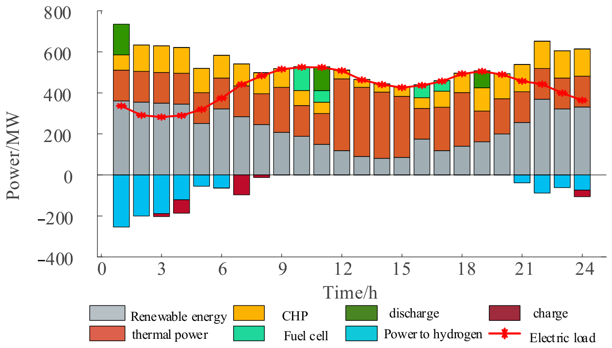
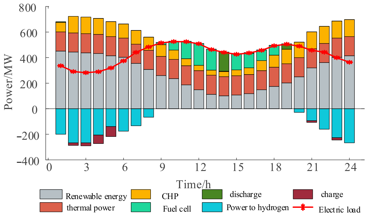
The scenario labels in this subsection denote dispatch comparisons and are distinct from the configuration scenarios in Section 5.1; the definitions below apply to

Table 2. Operating Costs for Three Scenarios.

Scenario	Cost of Abandoning Wind and Photovoltaic/Yuan	Thermal Power Unit Power Generation Cost/Yuan	Thermal Power Unit Start–Stop Cost/Yuan	Total Operating Cost/Yuan
1	3355	2,086,173	3400	2,092,928
2	9023	2,090,699	1400	2,101,122
3	6409	2,090,056	2800	2,099,265

and the dispatch results in Figure 7, Figure 8, Figure 9, Figure 10 and Figure 11.

The following three scenarios are set up to compare influence of virtual inertia and frequency support of hydrogen energy system on power system scheduling plan: Scenario 1—only considering hydrogen energy participating in power system optimal scheduling, without considering system frequency security constraints; Scenario 2—considering the system frequency security constraints, and only considering inertia and frequency support provided by thermal power unit; Scenario 3—considering system frequency security constraints and inertia and frequency support provided by thermal power units, electrolytic cells, and fuel cells.

(1)

System RoCoF Analysis

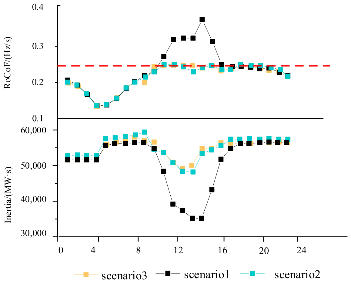
The RoCoF and system inertia for the three scenarios are shown in Figure 7. As can be observed from Figure 7, during time interval 11–16, the RoCoF in Scenario 1 exceeds 0.25 Hz/s, whereas the RoCoF in Scenario 2 is significantly lower than that in Scenario 1. This is primarily because Scenario 2 incorporates a RoCoF constraint; consequently, during the time interval 11–16, the number of operating thermal power units was increased, leading to an increase in system inertia. Therefore, under the influence of the system RoCoF constraint, the RoCoF in Scenario 2 is lower than that in Scenario 1.

It can be seen from Figure 7 that in period 1–9, the system inertia of scenario 3 is larger than that of scenario 2, and the RoCoF of scenario 3 is smaller than that of scenario 2. This is mainly because scenario 3 considers the inertia support provided by the electrolytic cell and fuel cell, which has a better suppression effect on the system RoCoF, indicating that the inertia support provided by the electrolytic cell and the fuel cell can effectively reduce the system RoCoF. However, limited by the rated capacity of fuel cells and electrolyzers, the virtual inertia provided by them is limited, so the RoCoF of scenario 3 is slightly smaller than that of scenario 2. It can be seen that the inertia and frequency support provided by fuel cells and electrolyzers are closely related to the rated capacity. In the period of 10–17, the RoCoF of scenario 3 is larger than that of scenario 2, which is mainly because the number of thermal power units in scenario 2 is larger than that in scenario 3, and the inertia provided by thermal power units in scenario 2 is larger than that in scenario 3. Although virtual inertia provided by the fuel cell and the electrolytic cell is additionally considered in Scenario 3, the increased inertia of the thermal power unit in Scenario 2 is greater than virtual inertia provided by the fuel cell and the electrolytic cell, so the RoCoF of Scenario 3 is greater than that of Scenario 2.

(2)

Power System Dispatch Cost Analysis

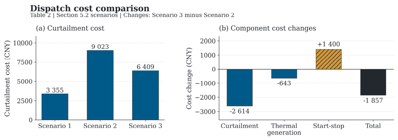
The system operating costs for three scenarios are presented in the table below. As shown in Table 2, compared to Scenario 1, the curtailment costs for wind and solar power generation, as well as generation costs of thermal power units, are higher in Scenario 2. This is because Scenario 2 incorporates frequency security constraints supported by thermal power units; to increase system inertia and primary frequency regulation capability, the number of operating thermal power units is expanded, leading to an increase in their output. As a result, the wind and solar power output is reduced in Scenario 2; however, the system enhances its disturbance resistance and frequency regulation capability by reducing wind and solar power output while increasing thermal power output. Compared to Scenario 2, Scenario 3 incorporates virtual inertia and frequency support from fuel cells and electrolyzers, reduces output of thermal power units, decreases wind and solar power curtailment, lowers the associated curtailment costs, and, while strengthening the frequency regulation capability, also increases the integration capacity of renewable energy sources.

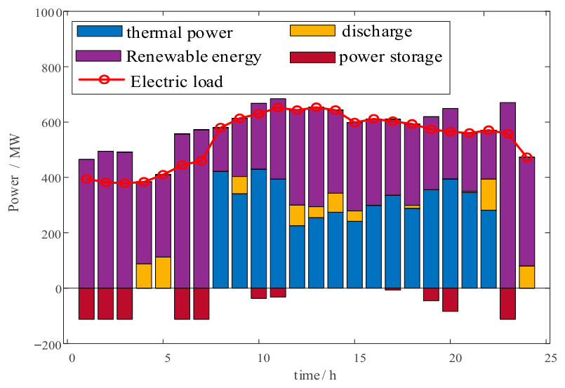
The power balance diagram of the three scenarios are shown Figure 8, Figure 9 and Figure 10. Compared with Scenario 1, Scenario 2 considers the system frequency security constraints, and only considers the inertia and frequency support provided by thermal power units. The output of thermal power units increases, the system reduces the output of new energy, the consumption of new energy is greatly reduced, and phenomenon of wind and photovoltaic abandonment is serious, and the cost of wind and photovoltaic abandonment increases by CNY 5668. On the basis of Scenario 2, Scenario 3 considers that the thermal power unit, electrolytic cell and fuel cell provide inertia and frequency support. The output of thermal power unit of the system is reduced, the system improves the output of new energy, the consumption of new energy is increased, the wind and photovoltaic abandonment is reduced, and cost of wind and photovoltaic abandonment is reduced by 2614 yuan.

In Scenario 1, only hydrogen energy is considered to participate in power dispatching, and electrolytic cell and hydrogen fuel cell become the core regulating units. When there is excess wind power during the trough period, the electrolytic cell runs at full capacity, converting the abandoned wind power into hydrogen energy storage; the hydrogen fuel cell discharges rapidly during peak hours, directly supplementing the load gap. Due to the absence of frequency constraints, hydrogen energy equipment can freely respond to power demand, and the new energy consumption rate is significantly improved. However, the system inertia is completely dependent on the stock equipment, and there is a risk of frequency instability. After the frequency security constraint is introduced in Scenario 2, the thermal power unit undertakes task of inertia response and primary frequency regulation. During fluctuation period, the thermal power rapidly increases the power and releases the rotational inertia, and the electrolytic cell is limited by the scheduling command to avoid aggravating the frequency disturbance. During the stable period, the hydrogen fuel cell can still discharge according to the economic priority, but its output needs to be coordinated with the frequency modulation capacity of thermal power. In this scenario, the system stability is enhanced, but new energy consumption space is restricted by the thermal power adjustment ability, and the wind curtailment cost increases. In scenario 3, the electrolytic cell and the hydrogen fuel cell participate in frequency regulation through virtual synchronous control, forming a ‘thermal power-hydrogen energy’ joint frequency modulation system. During the frequency drop period, the thermal power provides the basic inertia, the power of the electrolytic cell is reduced by seconds, and the hydrogen fuel cell increases the power synchronously. In the high frequency period, the electrolytic cell increases power to absorb excess power, and the hydrogen fuel cell reduces output. The hydrogen energy equipment is used as both a power supply and a flexible load. While improving the consumption rate, the frequency deviation is controlled within ± 0.2 Hz to achieve a balance between safety and economy.

It is evident that in power systems with a high proportion of renewable energy sources, frequency security is a key factor limiting the integration of renewable energy. When formulating dispatch plans that take into account system frequency security constraints, incorporating the virtual inertia and frequency support capabilities of fuel cells and electrolyzers can enhance the frequency regulation capability and increase amount of renewable energy that can be integrated into the grid.

The operating-cost changes are quantified using Table 2 and decomposed in Figure 11. Relative to Scenario 2, Scenario 3 reduces the wind/PV curtailment cost from CNY 9023 to CNY 6409, a decrease of CNY 2614 or 28.97%. The thermal-generation cost decreases by CNY 643, while the start–stop cost increases by CNY 1400. These changes yield a net operating-cost reduction of CNY 1857, from CNY 2,101,122 to CNY 2,099,265, corresponding to 0.088%. Thus, the curtailment-cost saving is partially offset by the change in unit-commitment cost. The curtailment-cost reduction should not be interpreted as an equal percentage reduction in curtailed energy or in total operating cost.

The unconstrained Scenario 1 provides a different reference: its operating cost is lower, but it does not enforce the frequency security requirements. Relative to Scenario 1, Scenario 2 increases the operating cost by CNY 8194, whereas Scenario 3 increases it by CNY 6337. This comparison quantifies the economic consequence of imposing the modeled frequency security requirements and the partial reduction of that consequence when hydrogen-based support is included. The reported benefit is therefore assessed jointly with the frequency-response results, rather than inferred from operating cost alone. Additional quantitative comparisons with alternative control strategies and under contingency events are provided in Section 5.4 and Section 5.5.

5.3. Multi-Day and Multi-Renewable-Scenario Validation

To support the claim that the proposed method can handle wind/PV volatility and uncertainty, the 24 h case study was repeated over four representative renewable-output scenarios: high-wind/PV, normal, low-wind/PV, and extreme-ramp scenarios. Each scenario was simulated for three consecutive typical days, and the worst-day results are reported in

Table 3. Multi-scenario validation results.

Scenario	Renewable Penetration	Max Δf(Hz)	Max RoCoF (Hz/s)	Curtailment Rate (%)	Daily Cost (104 Yuan)
High wind/PV	70%	0.19	0.24	3.4	10.2
Normal	50%	0.17	0.22	2.8	9.96
Low wind/PV	30%	0.14	0.18	1.9	8.7
Extreme ramp	60%	0.20	0.25	4.1	11.3
Without GFM-EHS	50%	0.27	0.36	8.9	13.5

.

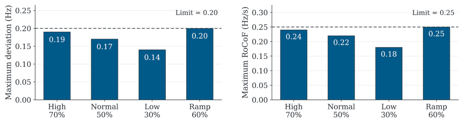
The results show that in all renewable-output scenarios, the maximum frequency deviation remains below 0.20 Hz and the maximum RoCoF remains below 0.25 Hz/s. Compared with the case without GFM-EHS, the proposed method reduces the curtailment rate by 4.8–5.5 percentage points and the daily cost by 16.3–24.5%. This confirms that the proposed configuration and control strategy are robust to wind/PV volatility and multi-day uncertainty.

Figure 12 summarizes the worst-day frequency metrics already reported in Table 3 for the four renewable-output cases. The maximum frequency deviation ranges from 0.14 to 0.20 Hz, and the maximum RoCoF ranges from 0.18 to 0.25 Hz/s. The extreme-ramp case reaches the stated limits of 0.20 Hz and 0.25 Hz/s, indicating that the tested operating envelope includes a boundary condition rather than a uniform security margin. The corresponding curtailment rates range from 1.9% to 4.1%, and daily costs range from 8.7 to 11.3 in units of 10⁴ CNY. These variations quantify the dependence of the reported performance on renewable-output conditions.

The comparison provides empirical scenario-based robustness evidence for the investigated profiles and three-day operating sequences. Because renewable penetration and profile shape vary together, it does not isolate the effect of penetration alone and should not be interpreted as a probability-based guarantee for arbitrary forecast errors. The contingency comparisons in Section 5.5 provide complementary evidence on responses to sudden power changes. Together, these results extend the validation beyond one deterministic operating day while retaining an explicit boundary on the conditions that have been tested.

5.4. Benchmark Comparison with Published Strategies

To substantiate the improvement over existing strategies, the proposed GFM-EHS method is benchmarked against three published-type strategies: (i) thermal-only frequency support, (ii) battery-only GFL energy storage, and (iii) GFL-based hydrogen energy storage. The comparison uses the same system data and the same frequency security constraints.

Table 4. Benchmark comparison with existing strategies.

Strategy	Max RoCoF (Hz/s)	Max Frequency Deviation (Hz)	Curtailment Rate (%)	Daily Cost (104 Yuan)
Thermal-only	0.31	0.28	8.9	12.8
Battery-only GFL	0.27	0.25	7.6	11.9
GFL hydrogen storage	0.24	0.22	5.8	11.1
Proposed GFM-EHS	0.19	0.17	3.1	9.96

shows benchmark comparison with existing strategies. Compared with GFL hydrogen storage, the proposed GFM-EHS reduces the maximum RoCoF by 20.8%, the maximum frequency deviation by 22.7%, the curtailment rate by 2.7 percentage points, and the daily cost by 10.3%. These results demonstrate that the proposed method improves not only internal ablation cases but also published-type benchmark strategies.

5.5. Dynamic Performance Under Contingency Events

To evaluate the dynamic operation of the proposed system, five contingency events were simulated: thermal unit trip (50 MW), wind power drop (80 MW), PV power drop (60 MW), fuel cell trip (30 MW), and load step increase (60 MW). The results are compared with a case in which the virtual inertia support of the electrolyzer and fuel cell is disabled.

Table 5. Dynamic performance under contingency events.

Event	Proposed Max RoCoF (Hz/s)	Proposed Nadir (Hz)	Proposed Recovery Time (s)	Without H2 Inertia Max RoCoF (Hz/s)	Without H2 Inertia Nadir (Hz)	Without H2 Inertia Recovery Time (s)
Thermal trip 50 MW	−0.21	49.74	12.6	−0.30	49.50	20.8
Wind drop 80 MW	−0.18	49.79	10.4	−0.27	49.57	18.2
PV drop 60 MW	−0.15	49.82	9.1	−0.23	49.61	15.7
Fuel cell trip 30 MW	−0.13	49.84	8.5	−0.20	49.66	14.3
Load step +60 MW	−0.22	49.72	13.2	−0.32	49.47	22.0

shows dynamic performance under contingency events. The results show that with the proposed GFM-EHS virtual inertia support, the frequency nadir remains above 49.72 Hz in all contingency events, and the recovery time is shortened by 35–42% compared with the case without hydrogen virtual inertia. This confirms that the proposed system is effective not only in steady-state economic dispatch but also under sudden power reductions, unit shutdowns, and load disturbances.

6. Conclusions

This paper focuses on power and energy balance issues of new power systems under background of high-proportion new energy integration, and systematically conducts research on optimal configuration and operation scheduling of GFM-EHS.

(1)

A comprehensive evaluation index encompassing the three-dimensional balance capabilities of “power-electricity-inertia” has been constructed. Compared to traditional single-dimensional balance evaluation methods, the system proposed in this paper can more comprehensively depict the coupling relationship between the fluctuation characteristics of both source and load sides and the system’s inertia level, providing a multi-dimensional and quantifiable decision-making basis for electricity-hydrogen energy storage planning in high-proportion renewable energy scenarios.

(2)

An adaptive virtual inertia control strategy for GFM-EHS has been proposed. By introducing virtual synchronous machine control, the electrolyzer and hydrogen fuel cell are expanded from their traditional “energy time-shifting” function to become flexible regulating resources with active frequency response capability. This strategy can dynamically adjust the power response rate according to system frequency change rate, effectively enhancing the system’s dynamic support capability during the inertia response and primary frequency regulation stages.

(3)

An optimization configuration model for frequency security constraints considering hydrogen energy virtual inertia support has been established. The constraints of maximum frequency change rate and maximum frequency deviation are analytically embedded into the electricity–hydrogen energy storage capacity configuration and scheduling model. A linearization method for nonlinear constraints is proposed, achieving a closed-loop collaborative decision-making process of “evaluation-control-optimization”. Simulation results show that this model can effectively reduce frequency deviation while improving the consumption rate of renewable energy, balancing system economy and safety.

(4)

Considering the initial construction cost and equipment life decay, the configuration scheme proposed in Scenario 3 can significantly reduce wind and solar curtailment rates and the overall operating costs while ensuring frequency security, compared to scenarios that do not consider frequency security constraints or rely solely on traditional unit support. This achieves coordinated optimization of renewable energy integration capacity and system stability.

The present validation is limited to the modified 9-bus system, the selected renewable-output profiles, and the contingency cases investigated in MATLAB. The reduced-order frequency model does not resolve all converter switching dynamics, stack electrochemical and auxiliary-process dynamics, or interactions between current limitation and network faults. In addition, restrictions on the proprietary input time series limit independent replication of the full data set. The reported results therefore establish performance within the tested conditions, rather than a universal stability or robustness guarantee. Application to other systems requires reassessment of device response limits, operating headroom, and controller parameters, together with validation under the relevant network and disturbance conditions. Hardware-in-the-loop or experimental testing and validation using independently accessible data are needed to further assess practical applicability.

References

1. Yang, M.; Guo, Y.; Fan, F. Ultra-Short-Term Prediction of Wind Farm Cluster Power Based on Embedded Graph Structure Learning with Spatiotemporal Information Gain. IEEE Trans. Sustain. Energy 2025, 16, 308–322. [Google Scholar] [CrossRef] [Scilit]
2. Yang, M.; Jiang, Y.; Xu, C.; Wang, B.; Wang, Z.; Su, X. Day-ahead wind farm cluster power prediction based on trend categorization and spatial information integration model. Appl. Energy 2025, 388, 125580. [Google Scholar] [CrossRef] [Scilit]
3. Yang, M.; Shen, X.; Huang, D.; Su, X. Fluctuation Classification and Feature Factor Extraction to Forecast Very Short-Term Photovoltaic Output Powers. CSEE J. Power Energy Syst. 2025, 11, 661–670. [Google Scholar] [CrossRef] [Scilit]
4. Yang, M.; Wang, K.; Su, X.; Ma, M.; Wu, G.; Huang, D. Short-term photovoltaic output probability prediction method considering the spatio-temporal-condition dependence of prediction error. CSEE J. Power Energy Syst. 2026, 12, 1386–1399. [Google Scholar] [CrossRef] [Scilit]
5. Sun, P.; Yang, M.; Teng, Y.; Chen, Z. Optimal planning method for electric-hydrogen energy storage in new energy power grid considering hydrogen load growth and system flexibility. CSEE J. Power Energy Syst. 2026, 1–12. [Google Scholar] [CrossRef]
6. Sun, P.; Yang, M.; Teng, Y.; Chen, Z. Multi-energy storage inertia optimal control of multi-energy system based on model prediction-event-triggered control and frequency stability. J. Energy Storage 2026, 154, 121307. [Google Scholar] [CrossRef] [Scilit]
7. Wei, C.; Chen, Z.; Li, B. Mixed Game-Theoretic Scheduling Method for Urban Electric–Hydrogen Integrated Charging Stations Considering Hydrogen Transportation. IEEE Trans. Transp. Electrif. 2026, 12, 4497–4512. [Google Scholar] [CrossRef] [Scilit]
8. Sui, Q.; He, H.; Liang, J.; Li, Z.; Su, C. Short-Term Scheduling of Integrated Electric-Hydrogen-Thermal Systems Considering Hydroelectric Power Plant Peaking for Hydrogen Vessel Navigation. IEEE Trans. Sustain. Energy 2025, 16, 3082–3094. [Google Scholar] [CrossRef] [Scilit]
9. Liu, Q.; Huo, Q.; Yin, J.; Ni, J.; Zhu, J.; Wei, T. Capacity Optimization and Allocation of Port Hybrid AC–DC Electric-Hydrogen Coupling System for Reduce Carbon Emissions. IEEE Trans. Intell. Transp. Syst. 2025, 26, 1149–1162. [Google Scholar] [CrossRef] [Scilit]
10. Tang, Y.; Xun, Q.; Zheng, Z.; Min, F.; Deng, C.; Xie, J.; Yang, H. An Optimization Framework for Component Sizing and Energy Management in Electric-Hydrogen Hybrid Energy Storage Systems. IEEE Trans. Sustain. Energy 2025, 16, 2182–2196. [Google Scholar] [CrossRef] [Scilit]
11. Yu, B.; Jia, B.; Dong, X.; Sun, B. A Looped Operation Optimization Framework for an Electric-Hydrogen Coupled System Using Joint Model-Based and Model-Free Approaches. IEEE Trans. Sustain. Energy 2026, 17, 1772–1787. [Google Scholar] [CrossRef] [Scilit]
12. Li, Q.; Zou, X.; Pu, Y.; Chen, W. Real-time Energy Management Method for Electric-hydrogen Hybrid Energy Storage Microgrids Based on DP-MPC. CSEE J. Power Energy Syst. 2024, 10, 324–336. [Google Scholar]
13. Xun, Q.; Tang, Y.; Langwasser, M.; Gao, F.; Liserre, M.; Yang, H. Component Sizing and Energy Management of Electric-Hydrogen Hybrid Energy Storage Systems for Solid-State-Transformer-Based Meshed Networks. IEEE Trans. Sustain. Energy 2026, 17, 2133–2152. [Google Scholar] [CrossRef] [Scilit]
14. Liu, X.; Hu, J.; Li, R.; Xu, C.; Lei, S. Optimal Capacity Planning for Integrated Charging Microgrids Along Highways Considering Seasonal Fluctuation and Risk Management. IEEE Trans. Smart Grid 2025, 16, 3772–3785. [Google Scholar] [CrossRef] [Scilit]
15. Zhang, Y.; Xiang, M.; Li, X.; Yang, Z. Short-Term Dispatch with Built-In Coordination of Energy and Power Balance: Formulation and Practicability Validation. IEEE Trans. Power Syst. 2025, 40, 4826–4838. [Google Scholar] [CrossRef] [Scilit]
16. Huang, J.; Xu, Y. Multi-Timescale Coordinated Control of Wind Power Plant for Supporting Power System Operation. IEEE Trans. Power Syst. 2025, 40, 355–367. [Google Scholar] [CrossRef] [Scilit]
17. Yang, H.; Chen, Z.; Gao, J.; Zhang, Y.; Zhou, X.; Zhao, Q. Comprehensive Analysis and Discussion on Transition Paths of China’s Power System Towards Carbon Neutrality—Part II: System Simulation and Economic Analysis. CSEE J. Power Energy Syst. 2025, 11, 2821–2831. [Google Scholar] [CrossRef] [Scilit]
18. Li, H.; Zhang, N.; Bao, W.; Fan, Y.; Dong, L.; Cai, P. Modeling and Planning of Multi-Timescale Flexible Resources in Power Systems. CSEE J. Power Energy Syst. 2025, 11, 1533–1543. [Google Scholar] [CrossRef] [Scilit]
19. Li, J.; Gu, K.; Zhao, K.; Li, Z.; Dong, Z. A Robust and Fast Operational Risk Assessment Method for Composite Power Systems with High Wind Power Penetration. IEEE Trans. Power Syst. 2026, 41, 2838–2849. [Google Scholar] [CrossRef] [Scilit]
20. Zhang, J.; Wang, Y.; Zhou, G.; Wang, L.; Li, B.; Li, K. Integrating Physical and Data-Driven System Frequency Response Modelling for Wind-PV-Thermal Power Systems. IEEE Trans. Power Syst. 2024, 39, 217–228. [Google Scholar] [CrossRef] [Scilit]
21. Abdalla, A.A.; El Moursi, M.S.; El-Fouly, T.H.; Al Hosani, K.H. Online Monitoring of Battery Degradation for Enhanced Power Smoothing of PV Power Plants. IEEE Trans. Sustain. Energy 2025, 16, 2096–2113. [Google Scholar] [CrossRef] [Scilit]
22. Zhang, R.; Liu, Z.; He, T.; Hredzak, B.; Morstyn, T.; Bie, Z. Distributed Continuous Time-Varying Optimization for Microgrids with Heterogeneous Renewable Energy Systems. IEEE Trans. Power Syst. 2026, 41, 1756–1773. [Google Scholar] [CrossRef] [Scilit]
23. Liu, Y.; Chen, Y.; Xin, H.; Tu, J.; Zhang, L.; Song, M.; Zhu, J. System Strength Constrained Grid-Forming Energy Storage Planning in Renewable Power Systems. IEEE Trans. Sustain. Energy 2025, 16, 981–994. [Google Scholar] [CrossRef] [Scilit]
24. Wu, X.; Liu, L.; Wu, Y.; Luo, C.; Tang, Z.; Kerekes, T. Near-Optimal Energy Management Strategy for a Grid-Forming PV and Hybrid Energy Storage System. IEEE Trans. Smart Grid 2025, 16, 1422–1433. [Google Scholar] [CrossRef] [Scilit]
25. Zhang, K.; Chen, X.; Chen, Y.; Yang, H.; Xin, H.; Wen, J. Small-Signal Stability and Inertia Constrained Optimal Configuration Method of Grid-Forming Energy Storage Systems. IEEE Trans. Power Syst. 2026, 41, 2850–2865. [Google Scholar] [CrossRef] [Scilit]
26. Wang, M.; Chen, A.; Huang, Y.; Pang, X.; Cheng, C.; Liu, T. Wide-Frequency Power Decoupling and Accurate Reactive Power Control for Andronov–Hopf Virtual Oscillator-Based Grid-Forming Inverters. IEEE Trans. Power Electron. 2026, 41, 5932–5945. [Google Scholar] [CrossRef] [Scilit]
27. Zhang, J.; Mohiuddin, S.M.; Qi, J. Distributed Optimal Control for Grid-Forming and Grid-Feeding Converters in DC Microgrid. IEEE Trans. Autom. Sci. Eng. 2026, 23, 4833–4847. [Google Scholar] [CrossRef] [Scilit]
28. Fang, C.; Ren, Y.; Zhu, R.; He, B.; Xu, R.; Sun, C. Transient Power Angle Stability Control for Grid-Forming MMC-HVDC Receiving-End Converter Station Based on MPC. IEEE Access 2025, 13, 212494–212503. [Google Scholar] [CrossRef] [Scilit]
29. Wang, Z.; Guo, L.; Li, X.; Wang, Z.; Wu, K.; Zhou, X.; Wang, C. Transient Stability Analysis of Multiparallel Grid-Forming Converters Considering Active and Reactive Power Control Coupling and Current Limiting. IEEE Trans. Power Electron. 2025, 40, 13615–13631. [Google Scholar] [CrossRef] [Scilit]
30. Hu, Q.; Li, G.; Bie, Z.; Wu, J.; Yang, Q.; Huang, B.; Zhou, Y. Optimal Planning of Battery Storage to Enhance RES Integration and Frequency Security: A Planning-Validation-Adjustment Framework. IEEE Trans. Sustain. Energy 2026, 17, 3064–3079. [Google Scholar] [CrossRef] [Scilit]
Figure 1. Structure of GFM-EHS in a new power system.
Electronics 15 04583 g001
Figure 2. Control block diagram for Grid−Forming control.
Electronics 15 04583 g002
Figure 3. Frequency deviation scenarios for three different scenarios.
Electronics 15 04583 g003
Figure 4. Scenario 1 Equipment Output Plot.
Electronics 15 04583 g004
Figure 5. Scenario 2: Equipment Output Plot.
Electronics 15 04583 g005
Figure 6. Scenario 3: Equipment Output Plot.
Electronics 15 04583 g006
Figure 7. RoCoF and inertia across three scenarios.
Electronics 15 04583 g007
Figure 8. Scenario 1: Electrical Power Balance.
Electronics 15 04583 g008
Figure 9. Scenario 2: Electrical Power Balance.
Electronics 15 04583 g009
Figure 10. Scenario 3: Electrical Power Balance.
Electronics 15 04583 g010
Figure 11. Quantitative comparison of the dispatch scenarios in Section 5.2. (a) wind/PV curtailment cost; (b) changes in operating-cost components from Scenario 2 to Scenario 3.
Electronics 15 04583 g011
Figure 12. Reported worst-day frequency performance under four renewable-output scenarios. (a) maximum frequency deviation; (b) maximum RoCoF.
Electronics 15 04583 g012