A Hybrid Deep Learning Framework for Non-Intrusive Load Monitoring

Abstract

In recent years, load disaggregation and non-intrusive load-monitoring (NILM) methods have garnered widespread attention for optimizing energy management systems, becoming crucial tools for achieving energy efficiency and analyzing power consumption. However, existing NILM methods face challenges in accurately handling appliances with multiple operational states and suffer from low accuracy and poor computational efficiency, particularly in modeling long-term dependencies and complex appliance load patterns. This article proposes an improved NILM model optimized based on transformers. The model first utilizes a convolutional neural network (CNN) to extract features from the input sequence and employs a bidirectional long short-term memory (BiLSTM) network to model long-term dependencies. Subsequently, multiple transformer blocks are used to capture dependencies within the sequence. To validate the effectiveness of the proposed model, we applied it to real-world household energy datasets: UK-DALE and REDD. Compared with suboptimal models, our model significantly improves the F1 score by 24.5% and 22.8%.

1. Introduction

With the depletion of fossil fuels and the increasingly severe energy crisis, China strives to peak emissions and achieve carbon neutrality [1]. Improving energy utilization efficiency and optimizing the power consumption structure have become critical factors in driving sustainable development. According to the 14th Five Year Plan for Electric Power Development report [2], China’s electricity consumption is projected to surpass 9.2 trillion kWh by 2025, with electric energy substitution exceeding 500 billion kWh. In the context of the ambition to achieve zero carbon dioxide emissions by 2050, the transformation of the power grid and the intelligent, efficient use of electrical resources are particularly crucial [3]. In addition, various energy-efficient appliances have entered the lives of people, but improper utilization of appliances has brought about many safety hazards [4]. NILM, as a crucial intelligent power-management approach, has been attracting increasing attention.

Load-monitoring techniques include intrusive load monitoring (ILM) and NILM [5]. ILM collects electricity usage data by installing sensors on each appliance individually, which allows for accurate monitoring. However, it is costly, complex to install, and raises concerns about user privacy. The concept of NILM was first proposed in 1982 [6]. It is primarily used for analyzing the aggregate load data of a specific area to obtain the load status of individual electrical appliances within that area [7]. In residential settings, NILM enables the energy consumption tracking of various appliances by monitoring and analyzing the total household total electricity usage data collected by smart meters. Compared with ILM, which requires monitoring loads by installing information acquisition equipment and sensing devices at each electrical appliance in the room of customers [8], NILM not only saves acquisition and installation costs of sensing equipment [9] but also significantly protects user privacy. By using smart meter data, NILM enables customers to understand the actual power consumption of each appliance and its contribution to the aggregate power consumption [10]. Such data play a crucial role in reducing carbon emissions and mitigating energy constraints [11]. NILM contributes to the precise analysis of electricity consumption patterns, the optimization of load forecasting and scheduling, and the provision of effective load management strategies for power utilities, thereby enhancing the stability of the power system and improving the efficiency of energy utilization. Therefore, the study of NILM is very important to maintain the stable operation of power systems [12].

The core process of NILM can be divided into four stages: data acquisition, feature extraction, event detection, and load monitoring. The key to the process is the extraction of effective features of residential appliance electrical use from the operational power data [13]. Recent studies have shown that NILM combined with machine learning can achieve excellent disaggregation results when an appropriate set of features is selected. For example, the study “Smart Non-Intrusive Appliance Load-Monitoring System Based on Phase Diagram Analysis” [14] demonstrates that careful feature engineering can significantly improve NILM performance. According to the type and characteristics of the sampled data, commonly used feature types can be classified into transient features and steady-state features [15]. Transient features are typically derived from high-frequency sampled data and can capture the dynamic changes that occur when appliances are switched on or off, such as current waveforms and harmonic information. However, acquiring such features places higher demands on data acquisition devices, data transmission, and storage. In contrast, steady-state features are based on low-frequency sampling and mainly include the root mean square values of voltage and current, as well as steady-state power. Most steady-state load characteristics can be directly sampled from the system or sensors [16]. Steady-state characteristics are easier to measure compared with transient features; steady-state characteristics are more widely applied in the existing research on NILM [17].

Since the introduction of NILM, research has focused on the load disaggregation problem [6]. In other words, load monitoring is implemented through load disaggregation techniques that aim to identify the operating states of individual electrical appliances. Subsequent research often employed methods such as mathematical optimization [18,19]. Most disaggregation techniques are based on signal processing techniques [20], supervised learning methods such as K-nearest neighbors (KNN), and unsupervised learning models like the hidden Markov model (HMM) [21]. Other common methods include factorial hidden Markov models (FHMMs) [22], graph signal processing (GSP) [23], and event-driven machine learning [24]. However, when dealing with a large number of appliances, the FHMM becomes computationally complex [25]. Machine-learning methods often require manual feature extraction [26]. Recent work has shown that, with carefully selected features, NILM combined with ML can achieve excellent disaggregation results. In particular, the study [14] highlights how feature engineering can significantly enhance performance. These handcrafted features typically include average power, peak power, power variation rate, switching event characteristics, and harmonic information. Their construction relies on prior knowledge of appliance operation patterns and domain-specific expertise.

Recently, intelligent algorithms have been widely employed in the domain of NILM with the introduction of artificial intelligence [27], such as bidirectional long short-term networks [13], temporal convolutional networks (TCNs) [28], and transformer models [29]. In addressing the NILM problem, research has focused on improving the performance of single-feature extraction. Zhong, Chen, and Lin [30,31] combined sequence-to-point (S2P), CNN, and BiLSTM deep networks to effectively extract features by training on the target appliance characteristics, resulting in an improved disaggregation accuracy. Yue and colleagues [32] applied the bidirectional encoder representations from transformers (BERT) model to NILM and introduced a penalty term in the loss function, enhancing disaggregation accuracy. However, the model’s performance decreased when dealing with appliances with multiple states. However, when addressing appliances with multiple operational states, the performance of existing models often deteriorates, failing to adequately capture the dynamic characteristics of complex loads. Furthermore, while certain methods enhance accuracy, they come with substantial computational overhead and resource demands, thus compromising their practical applicability. Consequently, a key challenge in current NILM research lies in improving the model’s ability to model multi-state appliances, while simultaneously optimizing computational efficiency without sacrificing disaggregation accuracy.

To overcome the aforementioned issues, this article proposes a hybrid CNN–BiLSTM–transformer architecture specifically designed for NILM tasks. NILM faces three key challenges: (1) extracting discriminative local features from aggregated power signals, especially for low-power and short-duration events; (2) modeling long-term temporal dependencies caused by appliance operation cycles and state transitions; and (3) capturing global contextual relationships within long power sequences. In the proposed framework, convolutional layers are employed to extract local temporal features and enhance the representation of short-term power variations. BiLSTM is used to capture long-term dependencies in both forward and backward directions, improving the modeling of appliance operation continuity. Furthermore, the transformer module introduces a global self-attention mechanism to model long-range contextual dependencies that are difficult to capture using recurrent networks alone. By integrating these complementary components, the proposed architecture effectively balances modeling capacity and computational efficiency, thereby improving the accuracy and robustness of load disaggregation. The main contributions of this paper are summarized as follows.

(1)

Although hybrid neural networks are common in NILM, the novelty of this work lies in a task-driven hierarchical design rather than simple model combination. The BiLSTM captures short-term bidirectional appliance switching patterns, while the Transformer models long-term dependencies and periodic behaviors at a higher feature level. This sequential integration is specifically tailored to NILM signal characteristics and differs from conventional parallel hybrid models.

(2)

Improved recognition of multi-state appliances and low-power devices by replacing ReLU with GELU activation for better dynamic power capture and enhancing decomposition accuracy through a hierarchical encoder–decoder structure with residual connections.

(3)

Experiments on the REDD and UK-DALE datasets demonstrate that the model outperforms existing models such as BERT, LSTM+, and Seq2Seq in core metrics like F1 score, MAE, and MRE. Specifically, the F1 score improved by 24.5% (REDD) and 116.12% (UK-DALE), while power estimation errors were reduced, proving its superiority and robustness in practical applications.

The rest of this article is organized as follows. Section 2 introduces the proposed method. Section 3 presents experimental results to validate the effectiveness of the proposed model. Finally, Section 4 provides a summary of the paper.

2. Method Framework

To address challenges in non-intrusive load monitoring (NILM), including poor disaggregation of low-power and multi-state devices, limited integration of local and global information, and high reconstruction errors, this paper proposes a hybrid deep-learning framework combining CNN, BiLSTM, and transformer modules. The CNN extracts local features to improve recognition of low-power appliances, the BiLSTM captures medium-term temporal dependencies to strengthen sequence modeling in complex and noisy load patterns, and the transformer introduces global attention to capture long-term dependencies and contextual relationships. While transformer models excel at modeling long-term dependencies, the combination with BiLSTM ensures more robust temporal feature representation in NILM scenarios. Deconvolution with nonlinear transformations further optimizes signal recovery and enhances load reconstruction. Experimental results demonstrate that the proposed framework significantly improves load disaggregation accuracy and robustness.

NILM aims to infer the operating states and corresponding power consumption of individual appliances using the total power load data collected by a smart meter. Since the total power consumption of a household can be viewed as the sum of the power consumption of all appliances, the essence of NILM is to decompose the power components of each appliance through time-series data analysis.

Assuming there are N appliances in a residential environment, the total power at time $t$ can be expressed as

$$\begin{array}{c}P\left(t\right)={\displaystyle \sum _{i=1}^N}{S}_i\left(t\right)P_i\left(t\right)+e\left(t\right)\end{array}$$

(1)

In this context, $P\left(t\right)$ denotes the total load power measured by the smart meter, $S_i\left(t\right)$ indicates the operating state of the $i$-th appliance (where 1 means it is “on” and 0 means it is “off”), and $e\left(t\right)$ represents the measurement error or noise interference. The NILM model learns from historical load data to identify the characteristic patterns of different devices, thereby establishing a mapping relationship from total power to appliance-level power consumption [9].

After training, the model can predict the energy consumption distribution of individual appliances based on the real-time observed total load, enabling fine-grained energy monitoring and consumption analysis.

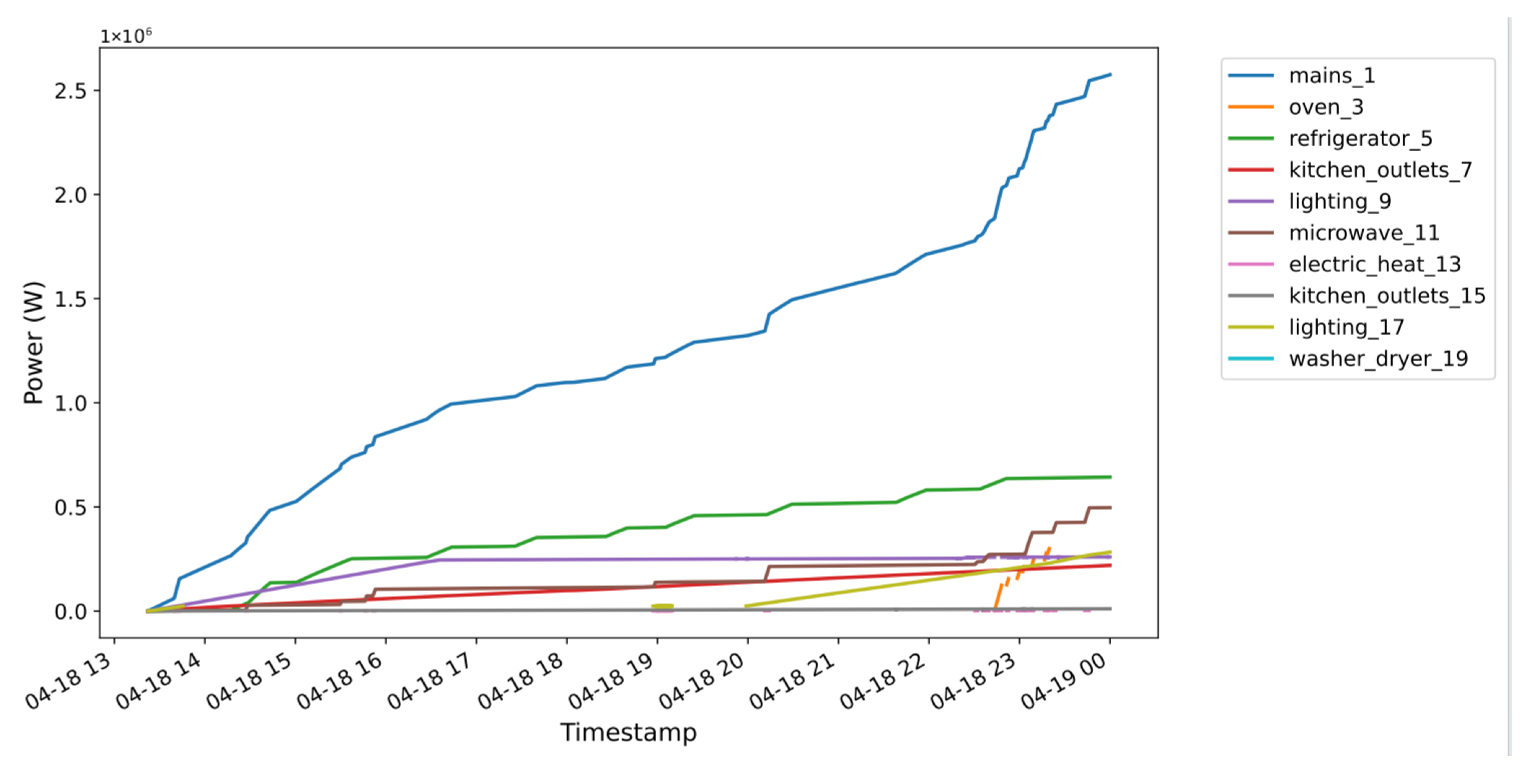
Figure 1 presents the cumulative power profiles of selected appliances in House 1, REDD low-frequency subset, after data cleaning and channel selection.

In general, researchers treat NILM as a sequence-to-sequence (Seq2Seq), sequence-to-subsequence, or sequence-to-point problem. The tasks typically include single-label or multi-label state classification and energy consumption prediction [33]. This paper chooses the Seq2Seq method for modeling the NILM task, primarily due to its ability to model temporal dependencies, prediction stability, and computational efficiency. Seq2Seq can output the entire power sequence over a time window, capturing the complete operational state of the appliance. Compared with Seq2Point, which predicts only a single point value, Seq2Seq reduces power estimation fluctuations and outperforms Seq2Subseq, which focuses only on partial subsequences and may lead to information loss. Additionally, Seq2Seq has a computational step of T ≈ L/W [25], which incurs lower computational costs compared with Seq2Point (T ≈ L) [25], making it more suitable for large-scale NILM tasks. It is particularly effective for devices with long operational characteristics, such as air conditioners and washing machines, improving the temporal consistency and generalization ability of power disaggregation.

The model employs a hierarchical encoder–decoder structure, combining 1D CNN, BiLSTM, and transformer to efficiently extract local and global features from power time-series data and perform energy disaggregation. The entire process can be divided into three stages: feature extraction (down sampling), temporal modeling (encoding), and signal reconstruction (decoding), as shown in Figure 2.

The model focuses solely on the load disaggregation task, which is currently the mainstream research direction, decomposing the total power load data into corresponding power sequences for target appliances. Initially, the input data is processed through a convolutional layer with a kernel size of 5 and an output channel number of 256. After the convolution layer, an L2-norm pooling layer (LPPool1d) is used for down sampling, further reducing the length of the time series while retaining useful features.

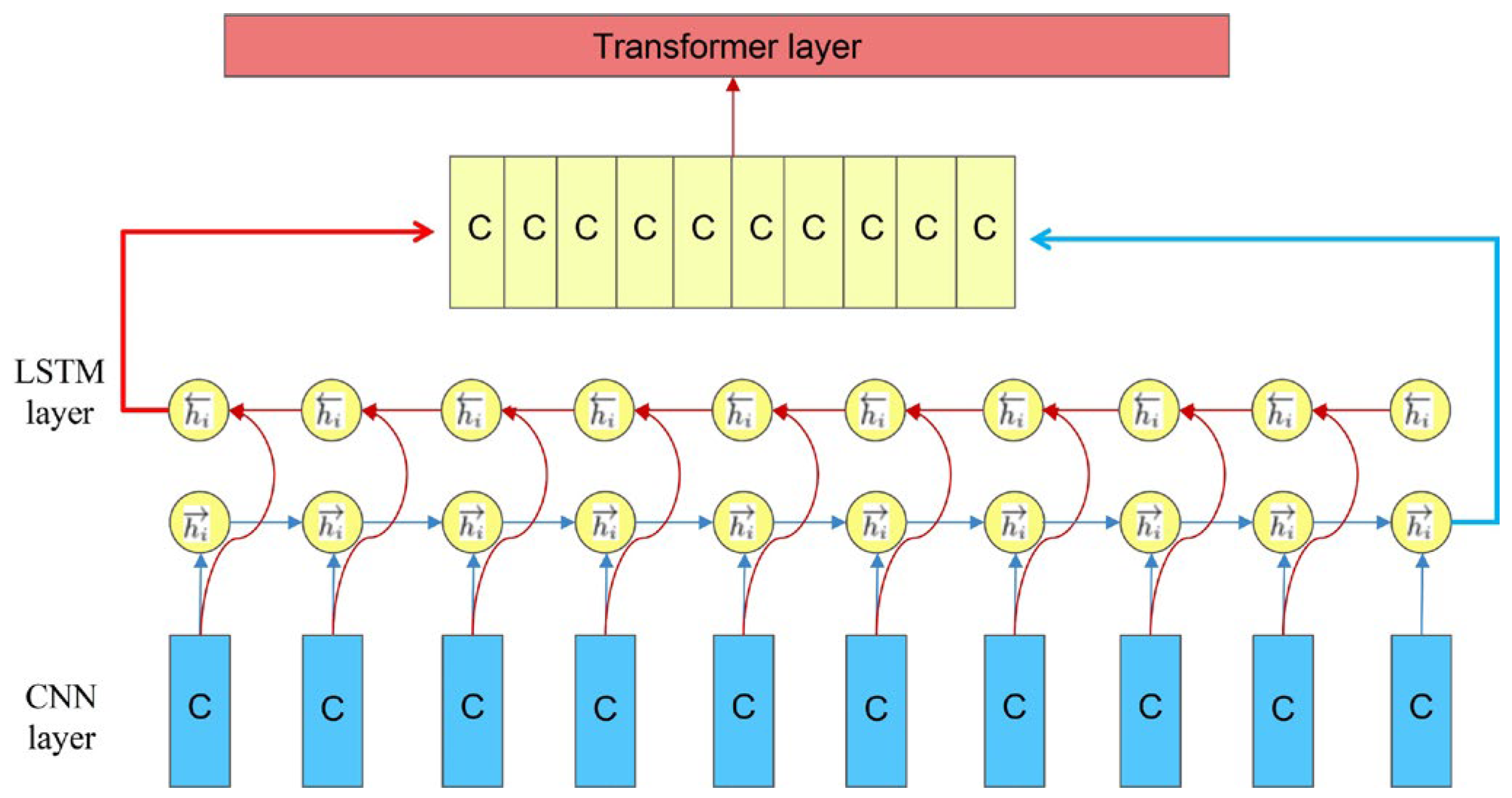
The time-series features extracted via convolution and pooling are reshaped to match the input format required by the BiLSTM layer, where the sequence length becomes the second dimension and the feature dimension becomes the third. The BiLSTM comprises two LSTM units that process the sequence in forward and backward directions, respectively. At each time step, the input feature vector has 256 dimensions.

As a bidirectional network, the BiLSTM generates two hidden states at each time step: one from the forward pass and one from the backward pass. Each LSTM direction has a hidden size of 128, resulting in a combined output dimension of 256. This configuration ensures compatibility with subsequent components of the model (such as the transformer module) and enables seamless information flow throughout the network, as shown in Figure 3. Therefore, the feature sequence input to the transformer block is

$$\begin{array}{c}{\mathit{X}}_{\mathrm{i}\mathrm{n}\mathrm{p}\mathrm{u}\mathrm{t}}=\mathrm{B}\mathrm{i}\mathrm{L}\mathrm{S}\mathrm{T}\mathrm{M} \mathrm{O}\mathrm{u}\mathrm{t}\mathrm{p}\mathrm{u}\mathrm{t}\in {\mathbb{R}}^{\left(batc{h}_{size},sequenc{e}_{length},256\right)}\end{array}$$

(2)

In Equation (2), ${\mathit{X}}_{\mathrm{i}\mathrm{n}\mathrm{p}\mathrm{u}\mathrm{t}}$ represents the input to the transformer model, derived from the output of the BiLSTM layer, where $batc{h}_{size}$ denotes the number of input sequences processed in parallel, $sequenc{e}_{length}$ represents the number of time steps in each input sequence, and 256 is the dimensionality of the output at each time step.

Transformers cannot directly capture temporal information; positional encoding is added to help the model understand the relative positions between time steps. In this work, positional encoding is implemented using learnable positional embeddings, which are treated as trainable parameters of the model and optimized jointly during training. These embeddings do not rely on additional input data and are added to the BiLSTM output before the transformer encoder. The specific relationship can be represented by

$$\begin{array}{c} Embedding=BiLSTM output+Pos Embed\end{array}$$

(3)

In Equation (3), $Embedding$ denotes the final input to the transformer encoder, $BiLSTM output$ encodes the temporal and contextual features extracted from the input power sequence, and $Pos Embed$ is introduced to incorporate information about the relative or absolute positions of time steps.

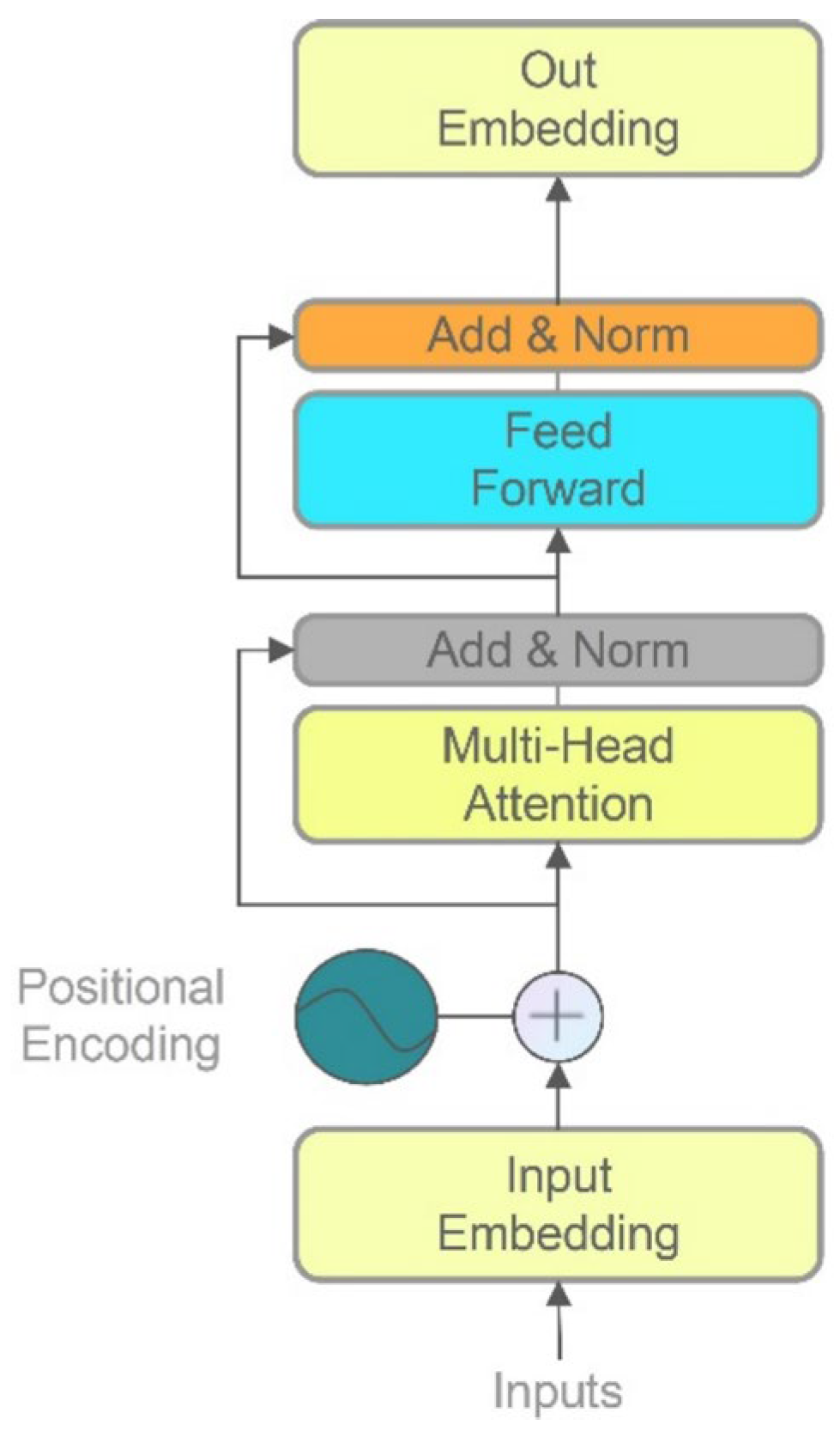
Then, the data is fed into four transformer encoders for deep feature extraction. Each transformer encoder consists of the following key components: a multihead self-attention layer, a feed-forward network (FFN), two layer-normalization layers (applied after the attention and FFN, respectively), and two residual connections, as shown in Figure 4.

In the feed-forward network, the original ReLU activation function is replaced with a GELU (Gaussian error linear unit). Unlike the rectified linear unit (ReLU), which hard-truncates negative values, the GELU smoothly attenuates negative inputs, allowing better gradient flow and improving training stability. This is particularly beneficial when processing data from appliances such as refrigerators with periodic start-ups or televisions that gradually adjust their power consumption. While the ReLU directly clips negative values—potentially discarding small signals—the GELU provides smooth transitions, ensuring that subtle load variations are preserved rather than completely lost.

The core computations in the multihead self-attention layer involve calculating attention scores and performing a weighted summation. The output can be formally expressed as

$$\begin{array}{c} \mathbf{Z}=\mathrm{A}\mathrm{t}\mathrm{t}\mathrm{e}\mathrm{n}\mathrm{t}\mathrm{i}\mathrm{o}\mathrm{n}\left(\mathit{Q},\mathit{K},\mathit{V}\right)=\mathrm{S}\mathrm{o}\mathrm{f}\mathrm{t}\mathrm{m}\mathrm{a}\mathrm{x}\left({\displaystyle \frac{\mathit{Q}{\mathit{K}}^{\mathrm{T}}}{\sqrt{{\mathit{d}}_{\mathit{k}}}}}\right)\mathit{V}\end{array}$$

(4)

In Equation (4), $\mathit{Q}$ (Query) represents the information at the current time step, while $\mathit{K}$ (Key) encodes the feature representations of all time steps. $\mathit{V}$ (Value) stores the actual feature information of each time step. The scaling factor ${\mathit{d}}_{\mathit{k}}$ (the dimensionality of the Key vector) is introduced to prevent excessively large attention scores, which could lead to unstable gradients. After passing through a linear layer, each input X with added positional encoding is projected into a $d_k$-dimensional space, generating the corresponding $Q,K,V$ representations:

$$\begin{array}{c} \mathit{Q}={\mathit{W}}_{\mathrm{Q}}\mathit{X},\mathit{K}={\mathit{W}}_{\mathrm{K}}\mathit{X},\mathit{V}={\mathit{W}}_{\mathrm{V}}\mathit{X}\end{array}$$

(5)

In Equation (5), $\mathit{X}$ represents the input feature sequence, ${\mathit{W}}_{\mathrm{Q}},{\mathit{W}}_{\mathrm{K}},{\mathit{W}}_{\mathrm{V}}$. These are three distinct learnable weight matrices, each used to generate the Query, Key, and Value vectors. Finally, the multiple heads are concatenated:

$$\begin{array}{c} \mathrm{M}\mathrm{u}\mathrm{l}\mathrm{t}\mathrm{i}\mathrm{H}\mathrm{e}\mathrm{a}\mathrm{d}\left(\mathit{Q},\mathit{K},\mathit{V}\right)=\mathrm{C}\mathrm{o}\mathrm{n}\mathrm{c}\mathrm{a}\mathrm{t}\left({\mathrm{h}\mathrm{e}\mathrm{a}\mathrm{d}}_1,{\mathrm{h}\mathrm{e}\mathrm{a}\mathrm{d}}_2,\dots ,{\mathrm{h}\mathrm{e}\mathrm{a}\mathrm{d}}_{\mathrm{h}}\right){\mathit{W}}^{\mathit{O}}\end{array}$$

(6)

In Equation (6), $\mathrm{C}\mathrm{o}\mathrm{n}\mathrm{c}\mathrm{a}\mathrm{t}\left({head}_1,{head}_2,\dots ,{head}_h\right)$ represents concatenating the outputs of all the attention heads, forming a larger vector that combines the results of the multihead attention. ${\mathrm{h}\mathrm{e}\mathrm{a}\mathrm{d}}_1,{\mathrm{h}\mathrm{e}\mathrm{a}\mathrm{d}}_2,\dots ,{\mathrm{h}\mathrm{e}\mathrm{a}\mathrm{d}}_{\mathrm{h}}$ are the outputs of multiple independent attention heads. Each attention head computes a weighted sum based on the attention mechanism applied to $\mathit{Q},\mathit{K},\mathit{V}.$ ${\mathit{W}}^{\mathit{O}}$ is a learnable linear transformation matrix that maps the concatenated multihead output back to the desired dimension.

In the encoding phase, the input data is down sampled through convolution and pooling operations. The transformer retains the down-sampled time steps, so during decoding, transposed convolution is applied for up sampling. Before inputting the data into the decoder, the data is reshaped to match the required format, with the hidden dimension and sequence length swapped. After recovering the time dimension through the transposed convolution layer, the data passes through a linear layer with a tanh activation to smooth the nonlinear mapping, ensuring continuity in appliance power data. Finally, a second linear layer without an activation function outputs the predicted power values for each time step of the target appliance, as the task is a regression problem. The final predicted result is

$$\begin{array}{c} \mathit{Y}={\mathit{W}}_2{\mathit{X}}_{\mathrm{L}\mathrm{i}\mathrm{n}\mathrm{e}\mathrm{a}\mathrm{r}1}+{\mathit{b}}_2\end{array}$$

(7)

where $\mathit{Y}$ represents the predicted power values for the target appliance at each time step, ${\mathit{W}}_2$ is the weight matrix of the second linear layer, and ${\mathit{b}}_2$ is the bias term of the second linear layer. ${\mathit{X}}_{\mathrm{L}\mathrm{i}\mathrm{n}\mathrm{e}\mathrm{a}\mathrm{r}1}$ represents the intermediate feature vector obtained from the previous nonlinear transformation and can be expressed as

$$\begin{array}{c} {\mathit{X}}_{\mathrm{L}\mathrm{i}\mathrm{n}\mathrm{e}\mathrm{a}\mathrm{r}1}=\tanh \left({\mathit{W}}_1{\mathit{X}}_{\mathrm{D}\mathrm{e}\mathrm{c}\mathrm{o}\mathrm{n}\mathrm{v}1\mathrm{d}}+{\mathit{b}}_1\right)\end{array}$$

(8)

In Equation (8), $\mathrm{t}\mathrm{a}\mathrm{n}\mathrm{h}$ is the hyperbolic tangent activation function, which introduces nonlinearity and helps capture the continuous variation in appliance power consumption; ${\mathit{W}}_1$ is the weight matrix of the first linear layer; ${\mathit{X}}_{\mathrm{D}\mathrm{e}\mathrm{c}\mathrm{o}\mathrm{n}\mathrm{v}1\mathrm{d}}$ is the output of the transposed convolution layer, representing the up-sampled time-series features; and ${\mathit{b}}_1$ is the bias term of the second linear layer.

3. Experimental Results and Discussion

3.1. Data Source

The experiments were conducted using the publicly available UK-DALE and REDD datasets for training and testing. REDD and UK-DALE are widely used datasets in the field of NILM. The REDD dataset has a relatively low sampling rate of 3 s and includes data from six U.S. households, with parameters such as voltage, current, active power, and reactive power. This dataset was used for preliminary testing of the model’s performance. On the other hand, the UK-DALE dataset includes data from five UK households, with parameters such as active power, current, voltage, and total power. The total power data is available in high-frequency (16 kHz) versions, which are suitable for transient analysis. Although the device-level data in UK-DALE is sampled every 6 s, which is slightly longer than that of REDD, it records data over a long period (up to approximately 2 years), making it suitable for long-term analysis. Thus, UK-DALE was selected as the primary dataset for in-depth analysis. In the REDD dataset, the focus was on appliances such as refrigerators, washing machines, microwave ovens, and dishwashers. In the UK-DALE dataset, the primary appliances studied were electric kettles, refrigerators, washing machines, microwave ovens, and dishwashers.

For the REDD dataset, data from House2, House3, House4, House5, and House6 were used for training and validation. The first 10% of the data from each house was allocated as the validation set, while the remaining 90% was used for training. The test set consisted of data from House1, which was not involved in the training process.

For the UK-DALE dataset, data from House1, House3, House4, and House5 were used for training and validation. Similarly, the first 10% of the data from each house was used as the validation set, and the remaining 90% as the training set. Data from House2 was used as the test set and was not involved in training. The data splits are summarized in

Table 1. Training, validation, and test set splits for REDD and UK-DALE.

Dataset	Train	Validation	Test
REDD	2, 3, 4, 5, 6 (90%)	2, 3, 4, 5, 6 (10%)	1
UK-DALE	1, 3, 4, 5 (90%)	1, 3, 4, 5 (10%)	2

.

3.2. Data Preprocessing

The raw data from both UK-DALE and REDD require specific preprocessing before being used for model training. First, appliance names and house numbers were checked to ensure validity. For each appliance, we verified whether it existed in the label file; if missing, the entries were filled with zeros. The time column was converted to datetime format to align all houses under a unified timestamp.

Next, the data were resampled at a frequency of 6 s, with values within each interval averaged. Missing values were handled using forward fill, which propagated the last valid observation to preserve temporal continuity. To avoid excessive filling, at most 30 consecutive missing values were allowed to be filled; longer gaps were excluded to prevent error accumulation. Rows containing missing values that could not be corrected were removed, and records where the total power equaled zero were deleted to filter out small fluctuations (e.g., standby power) or noise, thereby ensuring overall data quality.

Table 2. Missing-value statistics and handling.

Dataset	Total Duration	Missing-Value Ratio	Handling Method	Notes
UK-DALE	~2 years/house	3.10%	Forward fill/zero filling	Mostly short gaps in power data
REDD	~3–4 months/house	7.60%	Forward fill/row removal	Longer gaps due to meter faults

summarizes the missing-value statistics and handling strategies for both datasets. For abnormal appliance states, the data were truncated according to predefined power thresholds to ensure that power values did not exceed the preset maximum limits. In addition, specific turn-on/off thresholds and minimum operating times were applied for each appliance (as summarized in

Table 3. REDD appliance power thresholds and operating durations.

Appliance	Max Power Thres. (W)	On Thres. (W)	Min on Time (s)	Min off Time (s)
Refrigerator	400	50	60	12
Microwave	1800	200	12	30
Washing	500	20	1800	160
Dishwasher	1200	10	1800	1800

and

Table 4. UK-DALE appliance power thresholds and operating durations.

Appliance	Max Power Thres. (W)	On Thres. (W)	Min on Time (s)	Min off Time (s)
Refrigerator	300	50	60	12
Kettle	3100	2000	12	0
Microwave	1500	200	12	30
Washing	2500	20	1800	156
Dishwasher	2500	50	1800	1800

) to guarantee accurate device state detection. However, a maximum of 30 missing values can be filled to prevent excessive filling, which could introduce errors.

Next, rows containing missing values are removed, and records where the total power is zero are deleted to filter out small power fluctuations (such as standby power) or noise, ensuring data quality. For abnormal appliance states, the data is truncated based on predefined power thresholds to ensure the power values do not exceed preset maximum limits. Specific appliance turn-on and turn-off thresholds and minimum operating times are also applied, as shown in Table 2 and Table 3, to ensure accurate device state detection.

3.3. Experimental Setup

This paper compares the proposed model with three deep-learning models: BERT [32], Seq2Seq [33], and LSTM (LSTM+) [34]. All networks were modified to have the same input length and maximum hidden size and were trained under similar experimental settings until convergence. The experimental setup consists of a hardware configuration with a GeForce RTX 3090 GPU with 24 GB GDDR6X memory and an i9-10900X processor. On the software side, Python 3.10 is used, along with the PyTorch 2.4.1 deep-learning framework to implement the NILM models.

(1)

BERT [32]: A transformer-based model that handles temporal sequences, with parameters aligned to our experimental settings to ensure consistent performance.

(2)

Seq2Seq [33]: A CNN-based encoder–decoder framework that maps input sequences of appliance power readings to output sequences of predicted states, capturing temporal dependencies while reducing the impact of short-term fluctuations.

(3)

LSTM (LSTM+) [34]: A regularized LSTM architecture for appliance-level disaggregation, using stacked LSTM layers to model long-term temporal dependencies and maintain robustness to noisy power measurements.

The Adam optimizer is used to prevent model overfitting, and an early stopping strategy (20 epochs) is employed during training. For all appliances, a fixed sliding window size of 480 time steps is used to construct each input sample, which defines the input sequence length of the model, while the stride is set individually for different appliances as shown in

Table 5. Model hyperparameters.

Appliance	Stride	Batch Size	Learning Rate	Optimizer
Refrigerator	128	32	0.0001	Adam
Kettle	64	32	0.0001	Adam
Microwave	128	32	0.0001	Adam
Washing	256	32	0.0001	Adam
Dishwasher	128	32	0.0001	Adam

. The specific parameter settings are shown in Table 5.

The hyperparameters set for the refrigerator, washing machine, dishwasher, and microwave used in the REDD and UK-DALE datasets are the same as shown in the table above.

3.4. Performance Evaluation Metrics

In this study, to validate the feasibility and effectiveness of the model, we used F1-score (F1), mean absolute error (MAE), and mean relative error (MRE) as evaluation metrics. The F1-score is primarily used to assess the model’s classification ability for the on/off states of appliances. It combines precision and recall, providing a good measure of the model’s performance in appliance state detection. The formula is as follows:

$$\begin{array}{c} F1=2\times {\displaystyle \frac{Precision\times Recall}{Precision+Recall}}\end{array}$$

(9)

where $Precision$ represents the proportion of appliances predicted to be “on” that are actually “on.” $Recall$ represents the proportion of appliances that are actually “on” and correctly predicted as “on.”

$$\begin{array}{c} Precision={\displaystyle \frac{TP}{TP+FP}}\end{array}$$

(10)

$$\begin{array}{c} Recall={\displaystyle \frac{TP}{TP+FN}}\end{array}$$

(11)

where $TP$ represents the number of appliances that are actually “on” and correctly predicted as “on”; $FP$ represents the number of appliances that are actually “off” but incorrectly predicted as “on”; $FN$ represents the number of appliances that are actually “on” but incorrectly predicted as “off.” MRE is used to measure the size of the prediction error relative to the true value, making it suitable for appliances with different power levels, and is expressed as

$$\begin{array}{c} MRE={\displaystyle \frac{1}{N}}{\displaystyle \sum _{i=1}^N}{\displaystyle \frac{\left|{\widehat{y}}_i-y_i\right|}{y_i}}\end{array}$$

(12)

MAE is used to measure the magnitude of the error between the predicted power values and the true values, and is expressed as

$$\begin{array}{c} MAE={\displaystyle \frac{1}{N}}{\displaystyle \sum _{i=1}^N}\left|{\widehat{y}}_i-y_i\right|\end{array}$$

(13)

where ${\widehat{y}}_i$ is the predicted power value of the appliance; $y_i$ is the true power value of the appliance; and $N$ is the number of samples, the total number of time steps and appliance power data points involved in calculating the error. A higher F1-score indicates that the model can accurately detect the appliance state, while a lower MAE and MRE indicate that the model has higher precision and stability in the power disaggregation task.

Additionally, before conducting the formal experiments, we performed preliminary testing using Precision and Recall to quickly assess the model’s basic performance in appliance state detection. Since the NILM task involves multiple appliances, and the distribution of on/off states may be imbalanced across different appliances, using Precision and Recall during the early testing phase helps us evaluate whether the model suffers from false positives or false negatives, and provides a reference for the subsequent F1-score.

3.5. Model Complexity and Practical Considerations

The proposed model combines convolutional layers, BiLSTM, and transformer blocks to simultaneously capture short-term and long-term temporal dependencies in appliance-level load disaggregation. The computational complexity is dominated by the BiLSTM and transformer modules. Specifically, for an input sequence length of 480 and feature dimension of 256, the BiLSTM (two layers, 128 hidden units per direction) requires approximately 188 million multiply–add operations per input sequence, while the transformer blocks (two layers, two attention heads, a feed-forward hidden size of 1024) require approximately 155 million operations. The convolutional and decoding layers contribute negligible additional cost.

In addition to BERT, we also include TransUNet-NILM [25], a representative state-of-the-art NILM model, to benchmark both the performance and computational efficiency of our proposed approach under identical experimental conditions, including the same dataset, input sequence length, and hardware configuration.

Table 6. Runtime Comparison of Our-NILM and BERT, TransUNet-NILM on the same dataset.

Appliance	Window Size	Our-NILM (s)	BERT (s)	TransUNet-NILM
Refrigerator	480	95	89	216 s
Microwave	480	68	64	159 s
Washing Machine	480	146	137	314 s
Dishwasher	480	150	139	320 s
Average	480	114.75	107.25 s	252.25 s

presents the runtime comparison of Our-NILM with BERT and TransUNet-NILM. The measured inference times reflect the actual execution cost of processing an input sequence of length 480 for each appliance. While Our-NILM requires slightly longer runtime than BERT due to the additional BiLSTM and transformer modules, it remains practical for NILM applications, completing an input sequence in 114.75 s on average compared with 107.25 s for BERT. In contrast, TransUNet-NILM exhibits substantially higher inference times, averaging 252.25 s, indicating that Our-NILM achieves a favorable trade-off between computational efficiency and model complexity.

Table 6 and

Table 7. F1-score and MAE comparison of Our-NILM, BERT, and TransUNet-NILM on the same dataset under identical runtime conditions. (n this table and the following result tables, bold values indicate the best performance among the compared methods.).

	Our-NILM		BERT		TransUNet-NILM
	F1	MAE	F1	MAE	F1	MAE
Refrigerator	0.767	31.12	0.756	32.35	0.847	31.503
Microwave	0.512	17.30	0.451	17.58	0.351	18.429
Washing	0.603	31.88	0.559	34.96	0.304	35.711
Dishwasher	0.433	25.32	0.007	25.29	0.402	25.697
Average	0.579	26.40	0.443	27.54	0.476	27.835

summarize the performance and computational efficiency of Our-NILM compared with BERT and TransUNet-NILM under identical conditions. Our-NILM achieved an average F1-score of 0.579 and MAE of 26.40, outperforming BERT (F1: 0.443, MAE: 27.54) and showing comparable results to TransUNet-NILM (F1: 0.476, MAE: 27.84). For appliances like the washing machine, Our-NILM attained a higher F1 and lower MAE than both baselines, while for the refrigerator, it maintained a competitive MAE despite having a slightly lower F1 than TransUNet-NILM. Short-term high-power appliances (microwave, dishwasher) were robustly handled with a better F1 than BERT and an MAE similar to TransUNet-NILM. In terms of runtime, Our-NILM processed sequences in 114.75 s on average, slightly longer than BERT (107.25 s) but substantially faster than TransUNet-NILM (252.25 s), demonstrating a favorable trade-off between accuracy and efficiency.

The model can be deployed on edge devices with GPU support or cloud platforms, enabling near-real-time appliance state monitoring. Limitations include potential sensitivity to appliances or load patterns not present in the training data, as well as appliances with extremely short operation cycles or highly fluctuating power usage, which may result in slightly higher prediction errors. These factors suggest avenues for future improvement while confirming the practicality of the current approach.

3.6. Experimental Results

To further evaluate the effectiveness of the proposed hybrid architecture, we conducted comparative experiments between the proposed model and BERT-NILM under the same dataset partitioning, preprocessing procedures, and hyperparameter settings. Since BERT-NILM represents transformer-only architecture, this comparison directly examines whether introducing explicit sequential modeling brings additional benefits in NILM tasks. Experiment were carried out on the REDD dataset, where the refrigerator, washing machine, microwave, and dishwasher were selected as target appliances. Precision and Recall were adopted as the primary evaluation metrics to assess the model’s ability to accurately identify appliance operating states. The experimental results are summarized in

Table 8. Comparison of Precision and Recall on different appliances.

	Our-NILM		BERT
	Pre.	Rec.	Pre.	Rec.
Refrigerator	0.625	0.992	0.615	0.992
Microwave	0.581	0.457	0.545	0.385
Washing	0.445	0.932	0.594	0.594
Dishwasher	0.498	0.384	0.346	0.003

.

As shown in Table 8, the proposed model achieves higher recall for most appliances while maintaining competitive or improved precision compared with BERT-NILM. In particular, Recall improvement is more evident for appliances with short-duration high-power characteristics, such as the microwave, and for low-frequency appliances, such as the dishwasher, where the transformer-only model exhibits unstable or degraded performance. These results indicate that the proposed model is more effective at reducing false negatives while avoiding excessive false positives. Although transformer architectures are capable of capturing long-range dependencies through self-attention mechanisms, NILM tasks are characterized by strong temporal continuity and complex appliance state transitions. The inclusion of the BiLSTM module enables explicit bidirectional modeling of sequential dependencies, which complements the global attention mechanism of the transformer. This hybrid design improves the robustness in capturing appliance activation patterns and multi-state behaviors, leading to more reliable load disaggregation performance. Overall, the experimental results demonstrate that combining BiLSTM with a transformer enhances the model’s ability to handle diverse appliance characteristics in NILM scenarios, achieving a better balance between Recall and Precision compared with transformer-only approaches.

The performance of Our-NILM compared with BERT, LSTM+, and Seq2Seq is summarized in

Table 9. Comparison of evaluation results for four devices on the REDD dataset.

	Our-NILM			BERT			LSTM+			Seq2Seq
	F1	MRE	MAE	F1	MRE	MAE	F1	MRE	MAE	F1	MRE	MAE
Refrigerator	0.767	0.795	31.12	0.756	0.806	32.35	0.709	0.841	44.82	0.689	0.822	35.69
Microwave	0.512	0.057	17.30	0.451	0.057	17.58	0.604	0.058	17.39	0.378	0.060	18.59
Washing	0.603	0.028	31.88	0.559	0.022	34.96	0.128	0.020	35.73	0.274	0.042	36.12
Dishwasher	0.433	0.058	25.32	0.007	0.040	25.29	0.421	0.056	25.25	0.298	0.053	25.29
Average	0.579	0.234	26.40	0.443	0.231	27.54	0.465	0.243	30.79	0.409	0.244	28.92

and

Table 10. Comparison of evaluation results for five devices on the UK-DALE dataset.

	Our-NILM			BERT			LSTM+			Seq2Seq
	F1	MRE	MAE	F1	MRE	MAE	F1	MRE	MAE	F1	MRE	MAE
Refrigerator	0.825	0.695	20.76	0.766	0.732	25.49	0.174	0.956	43.74	0.718	0.758	29.20
Microwave	0.427	0.009	10.08	0.014	0.014	6.57	0.060	0.014	6.55	0.341	0.014	6.36
Washing	0.455	0.037	17.49	0.325	0.040	34.96	0.150	0.067	15.66	0.173	0.094	11.90
Dishwasher	0.751	0.033	14.87	0.667	0.049	16.18	0.605	0.033	36.36	0.560	0.069	25.43
Kettle	0.828	0.004	14.01	0.907	0.002	6.82	0.531	0.007	21.26	0.850	0.03	9.64
Average	0.657	0.155	15.44	0.535	0.167	18.00	0.304	0.215	24.71	0.528	0.193	16.50

. On the REDD dataset, Our-NILM achieved high F1-scores for most appliances, particularly the refrigerator and washing machine, indicating accurate on/off detection. In power estimation, Our-NILM showed a low MAE and competitive MRE, outperforming baseline models for the refrigerator and washing machine and maintaining robustness for short-term high-power appliances like the microwave and kettle.

On the UK-DALE dataset, our model outperformed the LSTM+ model, with the F1-score increasing by 116.12%. Our-NILM outperformed all baseline models on average across the F1-score, MAE, and MRE. The model achieved substantial improvements in the F1-score, particularly over LSTM+, and maintained the lowest average MRE (0.155) compared with BERT (0.167), LSTM+ (0.215), and Seq2Seq (0.193). For individual appliances, high-power devices such as the refrigerator, dishwasher, and kettle exhibited lower MREs than baselines, while short-duration appliances like the microwave had comparable MRE values, indicating stable and accurate performances across diverse appliance types.

Overall, our model combines the global feature extraction capability of the transformer with the sequential modeling ability of BiLSTM, achieving optimal performances in both state detection and power estimation tasks. Compared with other models, the model strikes a better balance between short-term high-power fluctuations and long-term stable loads. It outperforms BERT, LSTM+, and Seq2Seq models on the three core metrics—F1-score, MRE, and MAE—demonstrating a stronger generalization ability and robustness. Therefore, it is more suitable for NILM tasks and provides a more reliable solution for high-precision appliance identification and load disaggregation. 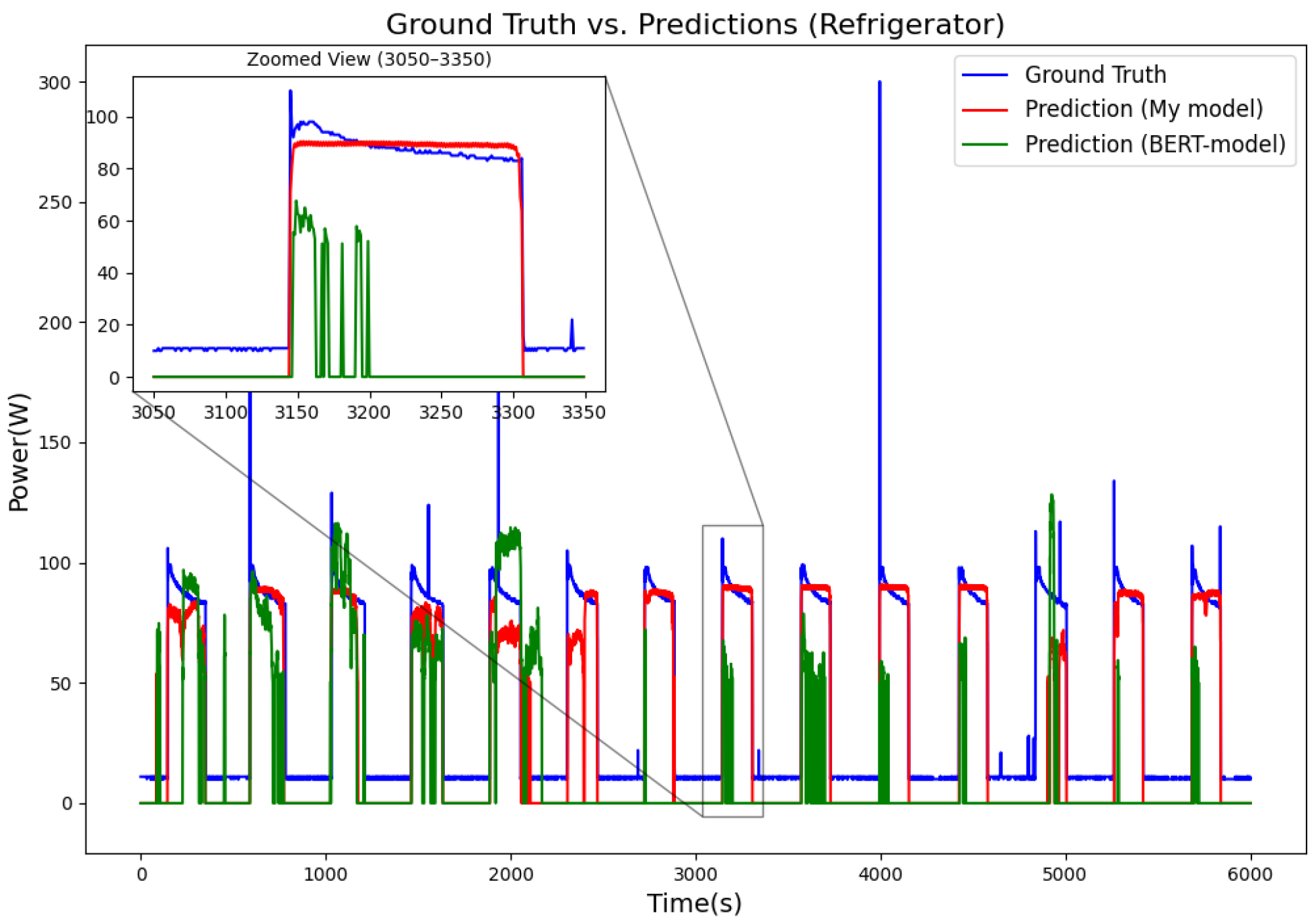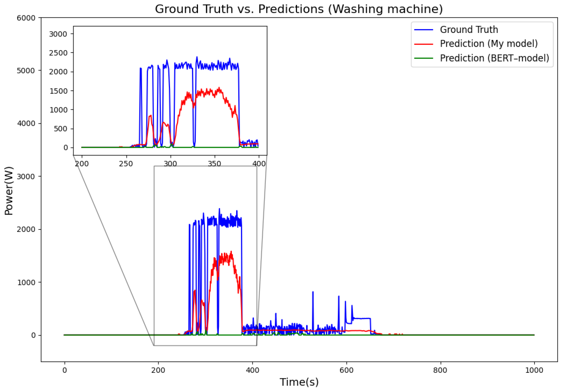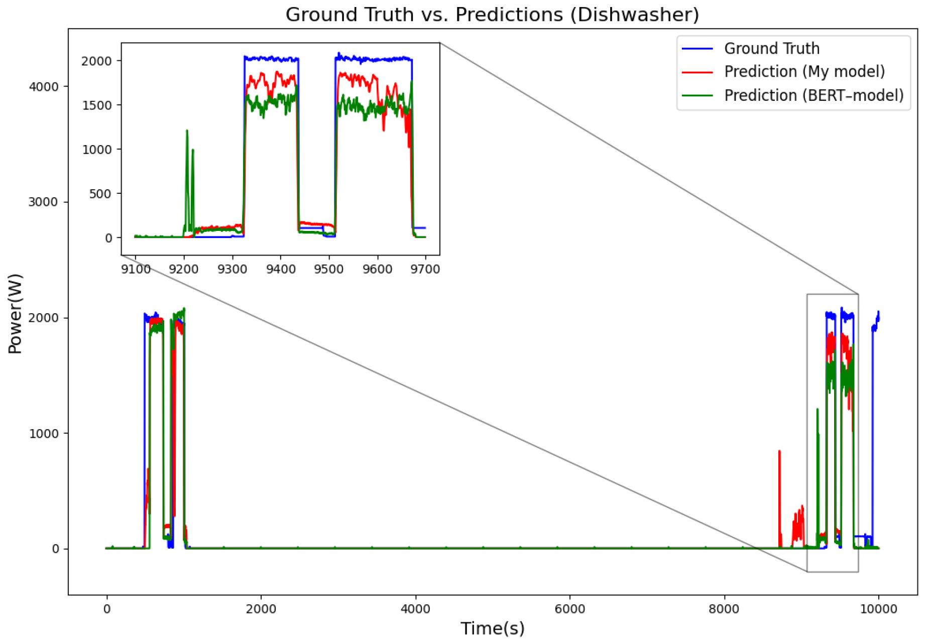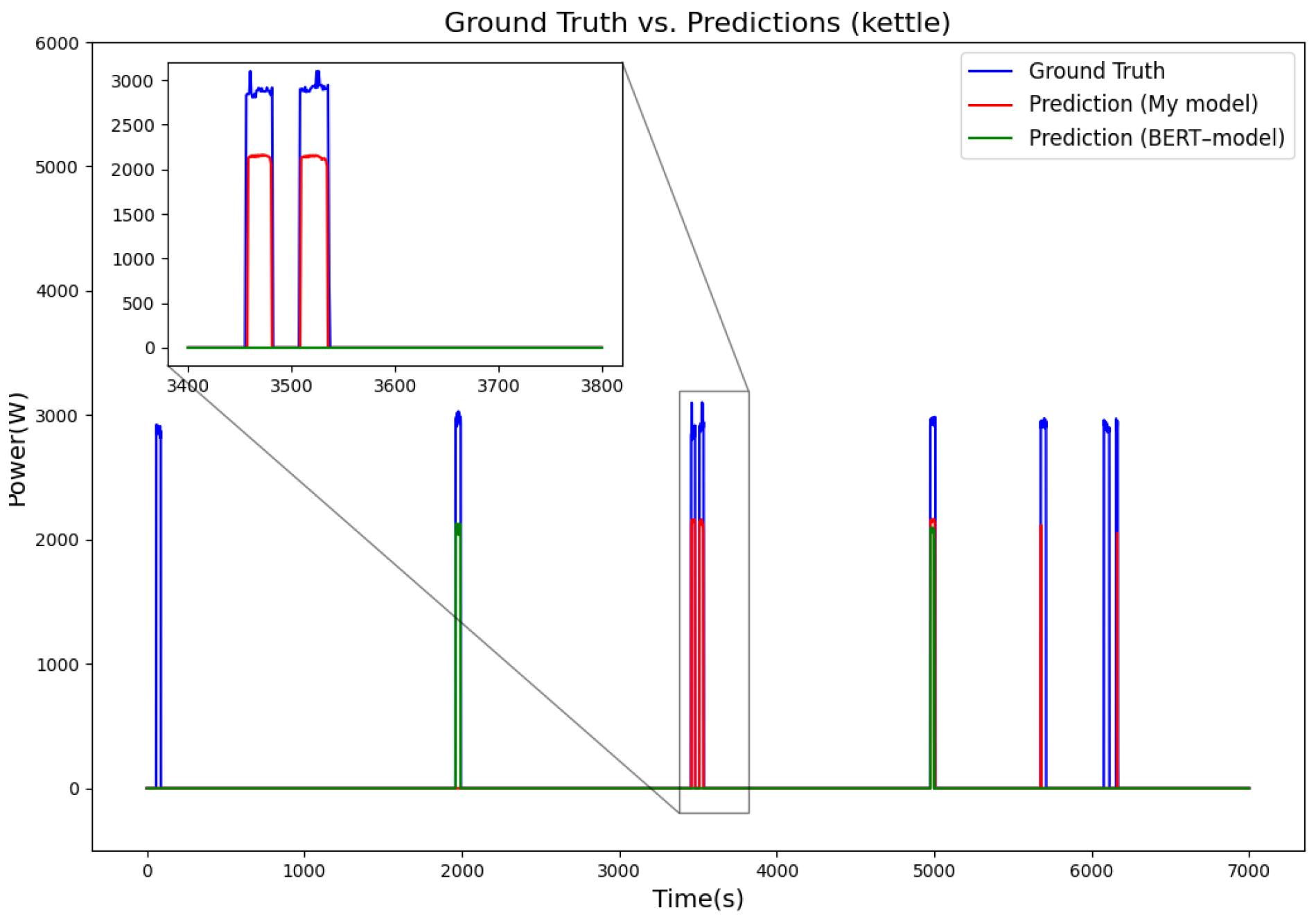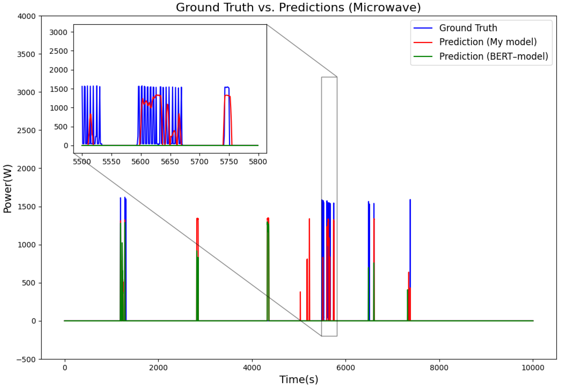Figure 5, Figure 6, Figure 7, Figure 8 and Figure 9 show the disaggregated power consumption curves for the refrigerator, kettle, dishwasher, and washing machine in the UK-DALE dataset. From the trend of the curves, it is evident that the power fluctuations predicted by our model are smoother, allowing it to more accurately track the actual load variations in the appliances. In contrast, the BERT model exhibits larger deviations in some cases, particularly during moments when the devices are turned on or off, where the power predicted by BERT often lags or fluctuates significantly. Additionally, the zoomed-in sections show that the model’s predicted power changes align more closely with the real values, whereas BERT tends to show abnormal spikes or false positives at certain moments. Compared with the BERT model, the model’s predictions are closer to the true values. Combining BiLSTM and transformer structures can not only extract key features of short-term power changes through BiLSTM but also capture long-term dependencies using the transformer. In contrast, although BERT relies on the transformer structure and can learn long-term dependencies between input sequences via self-attention mechanisms, it underperforms when dealing with short-term high-frequency load patterns. BERT lacks explicit sequential modeling capability, making it difficult to precisely capture the subtle changes during appliance on/off cycles, leading to a higher rate of false negatives for short-term high-power appliances (e.g., microwave, kettle).

4. Conclusions

Deep-learning-based NILM methods have made significant progress in smart meter data analysis. However, existing approaches still face certain limitations in power signal feature extraction, time-series modeling, and model generalization capabilities. Therefore, it is of great practical significance to develop an accurate and efficient NILM algorithm. In this paper, we propose HDL-NILM, which combines the advantages of transformers and BiLSTM, demonstrating superior performances in appliance power decomposition and load-monitoring tasks.

The model uses convolutional layers (CNN) for preliminary feature extraction, fully models the time-series dependencies through BiLSTM, and integrates a transformer to enhance global feature learning capabilities. The experiments are evaluated on the REDD and UK-DALE datasets. The results show that our model outperforms current state-of-the-art models in three core metrics: F1-score, MRE, and MAE, particularly exhibiting higher detection accuracy and lower power estimation errors for short-term high-power devices (e.g., microwaves) and long-term stable load devices (e.g., refrigerators, dishwashers).

Our model effectively captures the short-term power variation patterns of appliances through the BiLSTM structure, while the transformer module enhances the model’s ability to capture long-term dependencies, allowing the model to more accurately reconstruct appliance power curves. Additionally, the model uses residual connections and layer normalization to ensure gradient stability, improve training efficiency, and reduce computational cost. The experimental results demonstrate that the model improves the accuracy of NILM tasks and power prediction precision while maintaining high computational efficiency and generalization ability.

In future research, we plan to train and optimize the model on larger-scale datasets to enhance its adaptability in different household load environments. Furthermore, we will explore adaptive attention mechanisms and multi-task learning frameworks to further enhance the stability and versatility of NILM models, thereby advancing the practical application of NILM technology in smart homes and energy management.