Design and Implementation of a Model-Driven Embedded Simulation Control System for Diesel Engines

Abstract

To address the challenges of complex programming, high physicaltesting costs, and lengthy development cycles in conventional diesel engine controller development, this paper describes the design and prototype implementation of an embedded simulation control system for diesel engines, intended for early-stage controller algorithm pre-validation. The system is built around an STM32F407VE microcontroller and follows the model-driven development (MDD) paradigm. First, in accordance with the real-time and accuracy requirements of the simulation control system, core software modules—including real-time task scheduling, signal acquisition and processing, Ethernet communication, and host–target interaction—are designed to construct an embedded software framework that integrates simulation computation, signal sampling, command execution, and data exchange. Second, a modular diesel engine simulation model is developed in the MATLAB R2022b/Simulink environment and the graphical model is transformed and ported into embedded real-time C code via automatic code generation tools. Finally, an embedded real-time simulation verification platform is built. Distinct from our previous work on parallel power units, this study focuses on a single-engine diesel power system. Test results demonstrate that the proposed single-engine simulation platform can run the diesel engine model in real time on the target hardware and achieve closed-loop speed tracking under starting and multi-step command scenarios. The platform provides a low-cost, preliminary verification aid for early-stage diesel controller algorithm logic debugging and pre-parameter tuning. It should be highlighted that this platform is not intended for high-fidelity physical reproduction of real diesel engines. Quantitative model accuracy against real-engine dynamometer data remains to be established in future bench calibration campaigns.

1. Introduction

1.1. Research Background and Research Questions

In the field of marine propulsion systems, diesel engines are widely adopted in various marine power solutions owing to their stable power output, high efficiency, and strong adaptability [1,2]. However, a diesel engine comprises multiple strongly coupled subsystems—such as speed governing, turbocharging, and intake air heat exchange—which result in complex dynamic operating conditions and mutual coupling among parameters. Consequently, it is difficult to accomplish full operating-condition tuning and performance verification solely through conventional physical bench testing [3,4,5]. To reduce testing costs and shorten development cycles, numerical simulation and embedded real-time simulation technologies have progressively become core tools in diesel engine system development.

1.2. Limitations of Existing Methods

Currently, most diesel engine simulation studies rely on pure offline numerical simulation conducted in the MATLAB/Simulink environment. This approach can theoretically reproduce operating conditions and verify control algorithms. However, it is completely detached from the actual operating environment of embedded hardware, leading to issues such as software–hardware disconnection, insufficient real-time performance, and poor portability [6,7]. Meanwhile, software development for existing embedded simulation control systems for diesel engines mostly adopts traditional manual programming modes, which entail cumbersome development processes, heavy coding workloads, and long development cycles. Moreover, the resulting code suffers from poor generality, low readability, and limited scalability, making it difficult to meet the core requirements of synchronous multi-interface data interaction and real-time simulation computation. These deficiencies directly cause significant deviations between simulation control results and actual operating conditions, keep physical testing costs persistently high, and fail to satisfy the needs of engineering debugging and practical operation training.

1.3. Related Work

Model-driven development (MDD) methods have been widely adopted in embedded systems for automotive electronics and aerospace applications [8,9,10,11,12]. These studies demonstrate the effectiveness of MDD as a general-purpose methodology in diverse embedded-system domains and provide methodological support for the embedded diesel engine simulation in this work. For instance, the PELAB laboratory in Sweden proposed a continuous linearized model predictive control design method by combining OpenModelica and MATLAB [13,14]; the Jet Propulsion Laboratory of NASA conducted aviation system modeling based on model-based systems engineering and SysML, and developed model transformation and state analysis techniques [15,16]; and MDD techniques have also been successfully applied to controller development and cooperative path planning for multirotor UAVs and unmanned underwater vehicles [17,18]. However, research that systematically applies MDD to the simulation and embedded deployment of marine single diesel engines remains relatively scarce. Existing MDD-based diesel engine simulation studies either remain at the stage of offline model validation and algorithm testing in the Simulink environment, which cannot reach the actual hardware operating environment, or focus on cooperative power allocation of parallel power units while neglecting refined modeling of the complete thermodynamic dynamic characteristics of the single engine itself [1]. This research gap constitutes the core motivation of this paper.

With respect to marine engine simulation, digital-twin technology acts as the natural evolution direction for embedded simulation platforms. Liu proposed an intelligent self-adaptation framework for marine-engine degradation based on digital-twin models [19], which introduces online learning and degradation-monitoring capability for simulation models. Compared to their adaptive digital-twin platform, our work provides a low-cost, preliminary embedded simulation prototype without an online self-calibration function. Our platform can evolve toward a fully adaptive digital-twin solution by integrating self-calibration modules in future research. In addition, the self-calibrating simulation methodology proposed by Zhang [20], which combines physics-based models with data-driven correction layers, is highly relevant to our acknowledged challenge of model calibration against real-engine data and will be adopted in our future calibration work.

In the broader field of commercial simulation systems and embedded processor-in-the-loop (PIL)-type simulation platforms, commercial systemsm such as dSPACE, offer high fidelity and sub-millisecond real-time performance, but their hardware costs are high, and they are primarily intended for final electronic control unit (ECU) acceptance testing [19,20,21,22]. Low-cost solutions based on ARM Cortex-M microcontrollers have been validated in fields, such as power electronics, with hardware costs on the order of a few hundred RMB; however, they generally lack dedicated model libraries for diesel engine thermodynamic simulation [23,24,25,26].

Although single-engine diesel thermodynamic models are widely reported in the literature, most of these are desktop-oriented offline simulation. Systematic deployment, together with comprehensive measured real-time benchmarks on low-cost resource-constrained embedded hardware, for marine propulsion applications remains scarce.

1.4. Contributions and Scope of This Work

Against this background, this paper adopts model-driven development (MDD) as the core technical approach, and based on the already established hardware architecture [1], conducts the design and prototype implementation of an embedded simulation control system for diesel engines. Specifically, a modular and extensible diesel engine simulation model is built in MATLAB/Simulink. With embedded code generation tools, the graphical simulation model is automatically converted and optimized into executable embedded C code. By fully exploiting the hardware resources and peripheral interface features of the STM32F407VE microcontroller, core software functional modules—including real-time task scheduling, signal acquisition and processing, Ethernet communication, and host–target interaction—are developed. An integrated simulation control software system is then constructed, which is compatible with embedded hardware and combines simulation computation with control execution. On this basis, joint hardware–software online tests are carried out for typical operating conditions, such as engine startup/shutdown and speed governing, to verify system functionality and performance. This work provides a practical reference for the engineering development of embedded simulation platforms for marine propulsion systems. It is worth emphasizing that the reliability of this platform is demonstrated at two levels: (1) The whole MDD deployment workflow from Simulink model to embedded C code is verified via offline-online comparative tests; and (2) Comprehensive real-time performance tests including WCET, CPU utilization and communication latency prove stable scheduling behavior. However, these cannot substitute physical validation of plant model fidelity against real-engine hardware. Real-engine bench calibration is scheduled as key future work.

Our research group recently published a closely related study [1], in which a model-driven embedded simulation platform was designed for parallel dual-engine diesel power units, focusing on cooperative control between the two units. Although this paper shares the same MDD process and STM32 hardware platform with [1], the two works differ fundamentally in core content. Therefore, this study possesses independent and incremental innovative value. The specific differences are as follows:

System architecture: Reference [1] investigates a parallel dual-engine power architecture; this paper focuses on a single-engine power unit, which is the most mainstream configuration in marine propulsion systems.

Control logic: Reference [1] centers on cooperative speed and load allocation control between the two engines; this paper realizes closed-loop speed control for a single engine under typical operating conditions including startup/shutdown, idle speed stabilization, and multi-step speed command tracking.

Verification scope: Reference [1] only verifies the cooperative performance of parallel units; this paper conducts both offline Simulink simulation validation and online operation verification on the hardware target, with dedicated testing and analysis of the single-engine dynamic response characteristics.

To the best of our knowledge, few published studies have systematically documented the full MDD-based deployment of a complete single-engine diesel thermodynamic model onto a low-cost STM32F407VE platform with quantitative real-time performance measurements. This work represents a step toward filling that gap by providing an openly documented reference implementation. It should be clarified that without real-engine calibration, this platform cannot quantitatively reproduce all physical dynamic behavior of real diesel engines. Its value lies in preliminary algorithm debugging and pre-tuning at the early development phase. Control parameters obtained from this platform serve only as preliminary references and must be further tuned on a real-engine test bench for practical deployment. Different than pure methodological innovation, the novelty of this work lies in the systematic integration, adaptation, and quantitative verification of a mature MDD toolchain targeting a marine single-engine diesel scenario. The MDD workflow from Simulink to Embedded Coder to ARM target is well established in automotive and aerospace communities; our contribution does not propose new methodological paradigms but rather adapts and verifies these known tools for a specific marine single-engine use case. Partial hardware infrastructure and the overall MDD workflow are inherited from our previous dual-engine publication [1]. Nevertheless, we have rebuilt dedicated single engine-oriented sub-modules, revised internal software interfaces, and carried out full-set quantitative real-time performance measurements, which form the main incremental contributions of the present study.

It should be emphasized that this paper does not contribute new thermodynamic equations, control algorithms, or fundamental theoretical assumptions. The MDD toolchain, layered software paradigm, and RTOS scheduler are well-established existing technologies. The incremental value of this work is application-oriented: we implement the complete end-to-end deployment of a marine single-engine diesel thermodynamic model on low-cost STM32F407VE hardware and provide a full set of quantitatively measured real-time runtime benchmarks including WCET, task jitter, CPU utilization, and memory footprint for this specific marine propulsion scenario. Such systematic measured datasets are rarely reported in the literature for resource-constrained, mid-range microcontroller targets.

2. Overall Plan and Requirements Analysis

2.1. Core System Requirements

The software system of the proposed embedded simulation platform is developed and adapted based on a dedicated hardware architecture that has been completed previously. This hardware architecture is centered on an STM32F407VE microcontroller and is equipped with multiple types of peripheral interface circuits and signal-conditioning modules, thereby providing the physical carrier and underlying support for the operation of the software system. The software system in this design must simultaneously satisfy the dual requirements of functional completeness and performance compliance. It must fully cover the functional demands of the entire simulation control process while ensuring operational performance in the embedded environment, thus achieving efficient hardware–software coordination. The specific core requirements are as follows:

(1)

Signal acquisition and processing capability. The system must perform real-time acquisition and data parsing of digital command signals for diesel engine startup and shutdown, ensuring the authenticity and stability of input command signals, and providing a reliable data input foundation for subsequent simulation model computation and speed-control logic;

(2)

Full-process simulation computation capability. Relying on the diesel engine simulation model ported to the embedded platform, the system must perform real-time solving of the single-engine dynamic operating characteristics, fully reproduce the dynamic evolution of typical operating conditions, including startup, idle speed stabilization, and speed command changes, and output core simulation parameters, such as rotational speed in real time, ensuring that the simulation process on the embedded side closely approximates the actual diesel engine operating characteristics;

(3)

Ethernet and host computer communication capability. The software must implement driver adaptation for the Ethernet interface and communication protocol parsing, establish a data transmission channel between the simulation controller and the host computer, and upload simulation data—such as the diesel engine rotational speed computed by the embedded controller in real time—to the host computer;

(4)

High real-time performance capability. The simulation step size and command response latency must be strictly controlled to match the computational speed of the embedded hardware, guaranteeing high-speed and real-time data transmission, and ensuring temporal consistency between simulation computation, signal acquisition, and command execution;

(5)

Simulation computation accuracy. The calculation precision of simulation parameters must be ensured. Under subsequent bench calibration conditions, the deviation between simulation results and actual bench data should be controlled within a reasonable range. In the current offline and online verification stages, model usability is primarily evaluated through speed command tracking errors and the qualitative reasonableness of dynamic response trends;

(6)

Long-term operational stability. The software system must ensure no program crashes, no data drift, and no functional failures under continuous simulation conditions. Data interaction among modules must be smooth, and task scheduling must be orderly. Even in complex electromagnetic environments and multi-task concurrent execution scenarios, the system must maintain a stable operating state and consistent simulation performance;

(7)

Good scalability. The software architecture must adopt a modular design, supporting flexible addition or removal of functional modules and convenient modification of simulation parameters. It must also be compatible with different types of hardware peripherals and main control chips, requiring only minor modifications to the driver modules for hardware adaptation, thereby meeting the needs of future functional upgrades, operating condition expansion, and hardware iteration.

In summary, the core requirements of the software system are shown in Figure 1.

2.2. Overall System Architecture Design

To achieve modular decoupling, process-oriented scheduling, and efficient interaction of the embedded simulation control system for diesel engines, and in consideration of the embedded hardware architecture characteristics and the real-time requirements of simulation control, a hierarchical software architecture design philosophy is adopted. A six-layer software system is constructed, spanning from the simulation model to the underlying hardware, and from data computation to human–machine interaction. The layers are presented in order, as follows: the Simulation Model Layer, Real-Time Code Layer, Hardware Driver Layer, Task Scheduling Layer, Communication and Interaction Layer, and Application Layer. Each layer independently implements its core functions; information transfer and command interaction between layers are accomplished through standardized data interfaces. This forms a closed-loop software operation system of “model computation → code execution → hardware coordination → data feedback → application regulation,” which not only ensures the independence and maintainability of module development but also achieves deep adaptation and collaborative operation between software and hardware.

The Simulation Model Layer serves as the core computational foundation of the entire software system and is the “data source” of the embedded simulation. A modular diesel engine simulation model is built using MATLAB/Simulink and Stateflow, comprising sub-models such as the governor, turbocharger, and intercooler. Its core function is to solve for simulation parameters through mathematical models based on thermodynamics and control theory, according to input control commands and state data acquired from the hardware, and to output the simulation computation results to the Real-Time Code Layer. This layer interacts with the Real-Time Code Layer via standardized signal interfaces; the model-computed parameters and commands are transferred to the next layer in the form of digital signals.

The Real-Time Code Layer acts as the “bridge” between the simulation model layer and the underlying hardware execution. Relying on the MATLAB Embedded Coder toolchain, it automatically converts the graphical models from the Simulation Model Layer into embedded executable C code optimized for the ARM Cortex-M4 core, while performing code optimization and streamlining. Its core functions include receiving computation data and control commands from the Simulation Model Layer, performing signal parsing, format conversion, and data buffering at the code level, and passing the standardized digital commands and computation parameters to the Task Scheduling Layer. Simultaneously, it receives feedback data from the lower layer and transmits the data back to the Simulation Model Layer, enabling real-time model correction and closed-loop computation.

The Task Scheduling Layer serves as the “central scheduler” of the entire software system and is the core layer that guarantees the real-time performance of embedded simulation. Based on the computational characteristics of the main control hardware, a priority-driven task scheduling strategy is designed. Its core functions include unified management, priority assignment, and periodic scheduling of all real-time tasks within the system, ensuring that high-real-time tasks are executed with priority. Specifically, simulation computation tasks and hardware signal acquisition tasks are assigned high priority to guarantee the real-time responsiveness and continuity of model solving and command acquisition; Ethernet communication tasks and data buffering tasks are assigned medium priority, responsible for uploading and exchanging simulation data. The scheduling layer also coordinates data interaction among tasks, resolves resource contention and data conflicts during concurrent multi-task execution, ensures temporal consistency of task execution, and guarantees stable and reliable data transfer, thereby enabling orderly, efficient, and stable operation of the entire software system.

The present scheduling scheme adopts a classical fixed-period time-triggered strategy. Considering that the simulation computation task only occupies 3.1% of its 10 ms period (312.5 μs out of 10 ms), abundant computational headroom is available. Predefined sequential-synchronized control, combined with the event-triggered mechanism proposed by Cao, can be discussed for future optimization [27]. For long-term steady-state engine operation scenarios, event-triggered scheduling can eliminate redundant periodic computation, which helps to reduce power consumption or accommodate more complex sub-models. Event-triggered logic can be realized by modifying FreeRTOS task logic in our platform; it is not implemented in the current work.

The Communication and Interaction Layer serves as the data transmission channel between the embedded simulation platform and the host computer. Its core function is to establish data transmission between the controller and the host computer, receive the diesel engine simulation rotational speed data output from the Task Scheduling Layer, perform data encapsulation and transmission according to the Ethernet communication protocol, and upload the simulation data to the host computer visualization interface in real time. This provides the host computer with stable and continuous simulation operation data, ensuring the real-time performance and reliability of data uploading.

The Application Layer serves as the “human–machine interaction and functional presentation end” of the entire software system and is the final layer for simulation result display. Its core functions include receiving simulation data uploaded from the controller in real time, parsing and visualizing core operating parameters such as diesel engine rotational speed, and intuitively presenting the simulation operating conditions of the embedded platform through dynamic curves. It can clearly reflect the dynamic evolution of typical operating conditions such as engine startup and speed command adjustment, providing intuitive data support for system debugging, simulation experiments, and operating condition analysis. The overall software architecture design is shown in Figure 2.

3. Design and Implementation of Core Software Modules

3.1. Design of the Real-Time Task Scheduling Module

To satisfy concurrent multi-task execution and real-time demands of the diesel power unit embedded simulation platform, this module constructs a task scheduling architecture based on FreeRTOS. Hierarchical task partitioning, quantitative priority configuration, preemptive scheduling, and synchronous communication strategies are adopted to realize efficient system resource allocation and orderly multi-task execution, which guarantees real-time and reliable operation of the whole simulation control workflow.

The software system is decomposed into three core tasks according to the timing and functional requirements of diesel engine simulation control: simulation model computation, signal acquisition and processing, and Ethernet communication. The FreeRTOS preemptive priority scheduler enables high-priority tasks to preempt CPU resources, ensuring the timely responses of critical control functions.

The simulation computation and signal acquisition tasks are assigned high priority with a 10 ms period, undertaking real-time model solving and start/stop signal conditioning to secure real-time input and calculation. The Ethernet communication task has medium priority and a 20 ms period, handling data exchange between the target lower computer and host. It packages simulated speed data following predefined protocols and streams data to the host visualization interface for status monitoring.

Benefiting from the lightweight and configurable features of FreeRTOS, this module achieves accurate multi-task scheduling and coordination within the simulation controller. Core control tasks maintain response latency under 1 ms without task-switching deadlock or data interaction conflicts, satisfying the strict real-time and stability requirements of embedded diesel engine simulation control. The real-time task scheduling module is depicted in Figure 3.

3.2. Signal Acquisition and Processing Module

This module processes the startup and shutdown switching commands acquired via the hardware interface. The software performs real-time acquisition of logic-level states through GPIO ports, employs software debouncing and state latching mechanisms to eliminate transient interference signals, and conducts logic-level judgment to verify command validity, thereby ensuring accurate identification and stable response of the diesel engine startup and shutdown control commands.

To guarantee the real-time performance of command acquisition, the module operates in conjunction with the FreeRTOS real-time task scheduling mechanism. Signal sampling and state discrimination tasks are executed at a fixed period and the processed standardized command signals are sent in real time to the simulation model computation task via the inter-task data interaction mechanism, ensuring rapid response of the simulation system to external control commands. The design of the signal acquisition and processing module is illustrated in Figure 4.

3.3. Ethernet Communication Software Module

The Ethernet communication module acts as the primary external data transmission channel for this embedded simulation platform. Based on STM32F407VE hardware and FreeRTOS task scheduling, a dedicated communication driver is implemented with a lightweight TCP/IP stack to establish fixed data links between the embedded controller and host computer.

A unified transmission format and standardized data frame structure are defined to continuously upload core simulation variables, including real-time diesel engine speed. Taking advantage of high-speed Ethernet transmission, the module supports stable data streaming and satisfies the real-time visualization requirement for operating-condition data.

To improve transmission reliability and data integrity, the module integrates basic data verification and frame filtering to reject invalid redundant frames and lower transmission error risks. It exchanges data with the simulation computation module through FreeRTOS message queues. Simulation outputs are buffered in message queues and periodically retrieved and packaged by the communication task, enabling decoupled, interference-free operation of the communication function.

Ethernet communication performance is quantified via a point-to-point test between the host and target board. A total of 10,000 frames of 72-byte payload are transmitted at a 20 ms period over roughly 200 s. The results are listed in

Table 1. Ethernet communication performance metrics.

Metric	Value	Remarks
Communication protocol	TCP	Fixed connection
Number of test frames	10,000 frames
Average round-trip time	2.3 ms
Maximum round-trip time	6.8 ms
Packet loss rate	0%	No loss among 10,000 frames

.

No packet loss or CRC errors occurred across the 10,000-frame continuous test. The average round-trip latency is 2.3 ms, with a peak value of 6.8 ms. Both values are substantially smaller than the host refresh cycle; thus, communication delay imposes no observable influence on online monitoring.

It should be noted that this test is performed under controlled laboratory point-to-point connection. The results cannot reflect robustness under long-duration operation, host processing delay, link disconnection/reconnection, background network load, queue saturation, or latency distribution under variable loads. These items will be addressed in future reliability research.

This Ethernet module delivers low transmission latency and stable long-term data uploading, fully satisfying the real-time visualization demands of the diesel engine embedded simulation control system. The software architecture of the Ethernet communication module is illustrated in Figure 5.

4. Development and Validation of a Diesel Engine Simulation Model

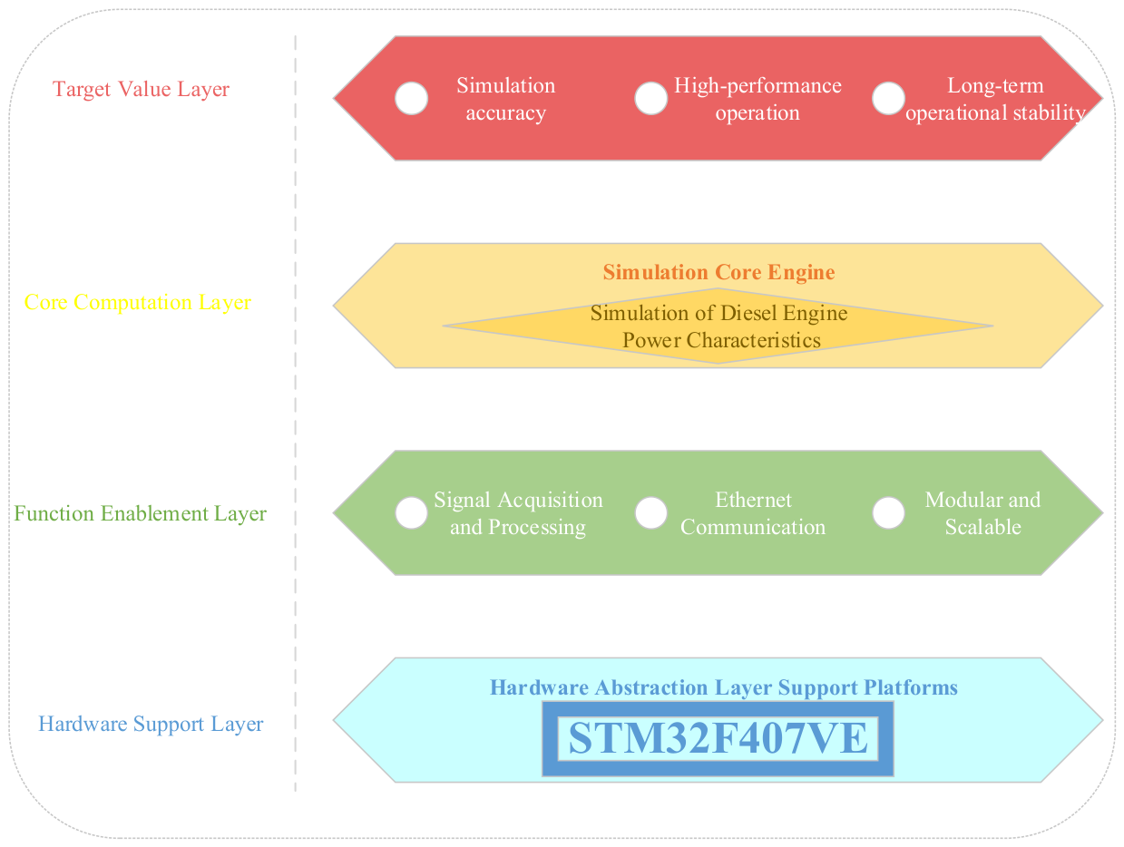
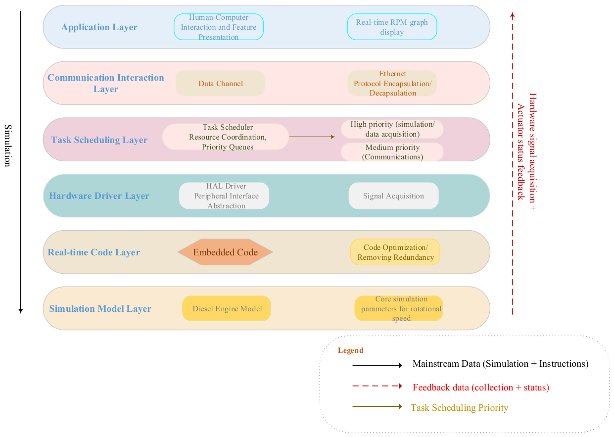
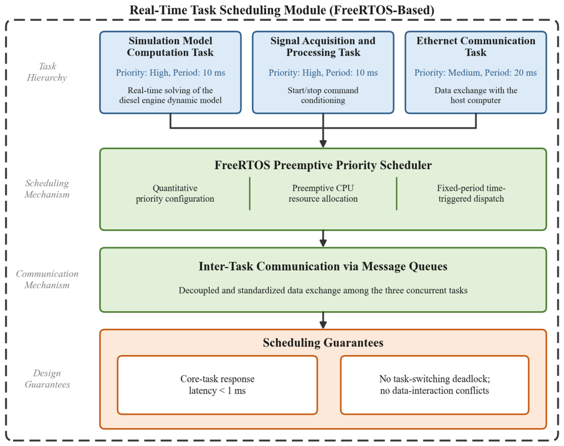
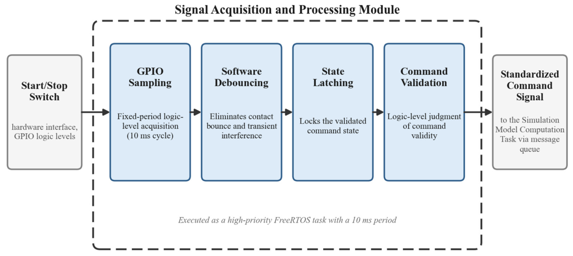
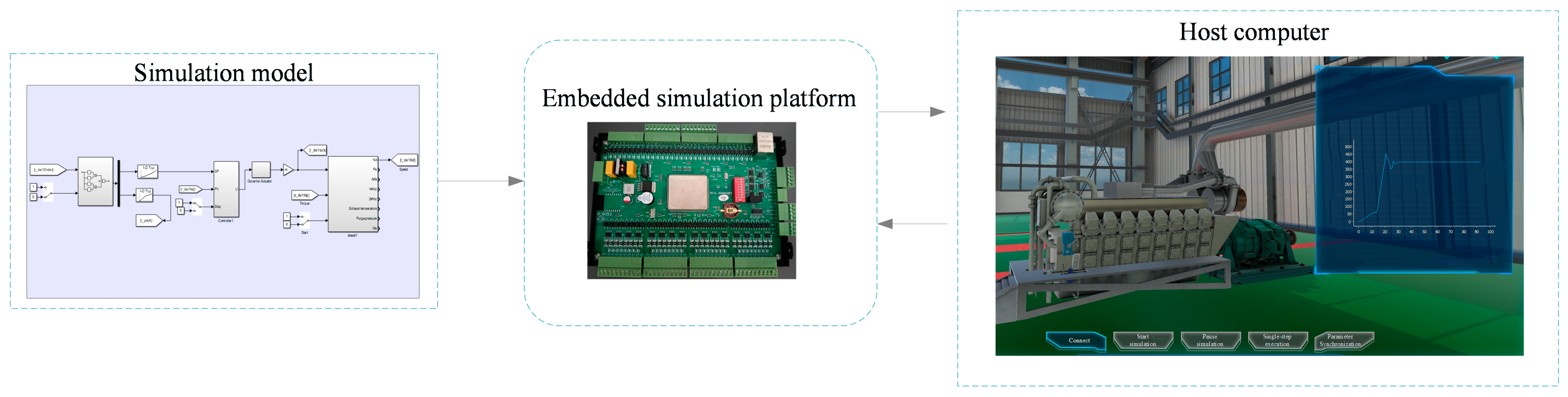
For the dynamic characteristics and speed-control logic of the diesel power unit, the MATLAB/Simulink environment is adopted to carry out modular design of the diesel engine simulation model. The modeling process follows the core principles of modular partitioning, standardized interfaces, and portability. An integrated simulation model is built around the intrinsic dynamic characteristics of the diesel engine, with each functional module independently computed to facilitate debugging and optimization. The model is encapsulated via unified interfaces, providing a standardized carrier for subsequent embedded automatic code generation.

The diesel engine model developed in this study is parameterized for a medium-speed, four-stroke marine diesel engine with the following key specifications: rated power of approximately 2000 kW, rated speed of 1000 rpm, cylinder configuration of eight cylinders in V-arrangement, bore of 280 mm, stroke of 320 mm, displacement per cylinder of approximately 19.7 L, and compression ratio of 14.5:1. This model is applicable to speed-control studies within the rotational speed range of 400–1000 r/min. Simulation results obtained outside this calibrated operating envelope should be interpreted with caution.

The diesel engine simulation model is decomposed into two core submodules—the governor and the turbocharger—according to the configuration of the power system. Additional dynamic modules, such as inertia, friction torque, and indicated torque, are integrated. The modeling is accomplished by combining theoretical equations with engineering data, thereby reproducing the diesel engine’s power output and transient dynamic response characteristics.

4.1. Governor Model

The governor, serving as the core unit for closed-loop speed control of the diesel engine, is modeled using an incremental PID control algorithm. By detecting the deviation between the actual rotational speed and the setpoint speed in real time, the algorithm synthesizes proportional, integral, and derivative actions to output a fuel adjustment command, thereby achieving precise and stable speed control of the diesel engine and effectively suppressing speed fluctuations caused by sudden load changes and operating condition transitions. The mathematical model of the incremental control algorithm is given as follows:

$$\Delta u(k)=K_p[e(k)-e(k-1)]+K_{i}e(k)+K_d[e(k)-2e(k-1)+e(k-2)]$$

(1)

$$u(k)=u(k-1)+\Delta u(k)$$

(2)

In the equation, $\Delta u(k)$ is the control increment for the $k$th sample; $K_p, K_i, K_d$ are the proportional, integral, and derivative coefficients, respectively; $e\left(k\right), e(k-1), e(k-2)$ are the speed errors for the $k, k-1, k-2$ samples, respectively; and $u(k), u(k-1)$ are the fuel control output commands for the $k, k-1$ samples, respectively. The proportional coefficient $K_p$ is set to 0.05, the integral coefficient $K_i$ to 0.02, and the derivative coefficient $K_d$ to 0.01.

4.2. Turbocharger Model

The turbocharger sub-model is constructed based on aerothermodynamic equations and rotor dynamics equations to simulate the energy conversion and rotational speed response characteristics of the compressor and turbine. The speed response of the turbocharger rotor is governed by its dynamic equation:

$${\displaystyle \frac{d{n}_t}{dt}}={\displaystyle \frac{30}{\pi }}\cdot {\displaystyle \frac{1}{I_t}}(M_t-M_k)$$

(3)

In the equation, $n_t$ is the turbocharger rotational speed; $I_t$ is the moment of inertia of the turbocharger rotor; $M_t$ is the turbine torque; and $M_k$ is the compressor load torque.

The turbine torque is derived from exhaust energy conversion and its calculation formula is:

$$M_t={\displaystyle \frac{30{\eta }_T{G}_t}{\pi n_t}}\cdot {\displaystyle \frac{k_t}{k_t-1}}\cdot R\cdot T_t\left[1-{({\pi }_t)}^{{\displaystyle \frac{k_t-1}{k_t}}}\right]$$

(4)

In the equation, ${\eta }_T$ is the turbine efficiency; $k_t$ is the exhaust adiabatic index, $k_t=1.33$; $R$ is the air gas constant; ${\pi }_t$ is the turbine pressure ratio; $T_t$ is the turbine inlet exhaust gas temperature; and $G_t$ is the exhaust mass flow rate.

The exhaust mass flow rate $G_t$ flowing through the turbine can be determined from the nozzle flow characteristics as follows:

$$G_t={\beta }_t\cdot F_t\cdot {\displaystyle \frac{P_{ti}}{\sqrt{R{T}_T}}}\cdot \sqrt{{\displaystyle \frac{2k_t}{k_t-1}}[{({\pi }_t)}^{-{\displaystyle \frac{2}{k_t}}}-{({\pi }_t)}^{{\displaystyle \frac{k_t+1}{k_t}}}]}$$

(5)

In the equation, $F_t$ is the effective flow area of the turbine nozzle, and ${\beta }_t$ is the nozzle flow coefficient under the corresponding operating conditions, which is related to the turbine pressure ratio.

The load torque $M_k$ at the compressor end reflects the work consumed by the compressor in compressing air and its expression is given as:

$$M_k={\displaystyle \frac{30G_k}{\pi {\eta }_k{n}_t}}\cdot {\displaystyle \frac{k}{k-1}}\cdot R\cdot T_0\left[{({\pi }_k)}^{{\displaystyle \frac{k-1}{k}}-1}\right]$$

(6)

In the equation, $G_k$ is the air mass flow rate at the compressor inlet; $k$ is the adiabatic index of air, $k=1.4$; ${\eta }_k$ is the compressor efficiency; $T_0$ is the compressor inlet air temperature; and ${\pi }_k$ is the compressor pressure ratio.

Both the compressor efficiency and the compressor pressure ratio are nonlinear parameters that vary dynamically with operating conditions. The data are obtained from the steady-state bench-test characteristic curves of the turbocharger.

The flow characteristics of the compressor are described by its flow function:

$$G_k={\displaystyle \frac{V_k{P}_0}{R{T}_0}}$$

(7)

In the equation, $V_k$ is the volumetric air flow rate at the compressor inlet and $P_0$ is the air pressure at the compressor inlet.

The compressor torque model is established according to Equations (6) and (7).

4.3. Diesel Engine Prime Mover Dynamics Model

The diesel engine prime mover model addressed in this paper is primarily concerned with describing the variations in output torque and rotational speed as functions of rack displacement, rather than the specific details of internal combustion parameters. Under the dynamic operating conditions of the diesel engine, the angular acceleration of the crankshaft is jointly governed by the net driving torque and the moment of inertia. Based on the rigid-body rotation law, the power unit is treated as a single-degree-of-freedom rotational system and the dynamic equilibrium equation is formulated as Equation (8):

$$J{\displaystyle \frac{d\omega }{dt}}={\displaystyle \frac{2\pi I_e}{60}}\cdot {\displaystyle \frac{d{N}_d}{dt}}=M_e-M_B-M_f$$

(8)

In the equation, $J$ is the equivalent moment of inertia of the diesel engine referred to the crankshaft; $\omega$ is the crankshaft angular speed; $I_e$ is the shaft system moment of inertia, set as $224{0 \mathrm{kg}·\mathrm{m}}^2$; $N_d$ is the diesel engine rotational speed; $M_e$ is the effective output torque of the diesel engine; $M_B$ is the braking torque of the load; and $M_f$ is the friction torque of the diesel engine.

The relationship between $M_f$ and $N_d$ is given as follows:

$$M_f(N_d)=\left\{\begin{array}{l}130,0<N_d<60\\ ({\displaystyle \frac{7121}{700}})N_d,N_d\ge 60\end{array}\right.$$

(9)

To achieve quantitative modeling of the effective output torque of the diesel engine, a mathematical relationship between the effective output torque and the combustion process, as well as the mechanical losses, is established based on the principle of fuel energy conservation. The effective output torque is derived by subtracting mechanical losses from the indicated torque, and its theoretical expression is given by Equation (10):

$$M_e=M_i{\eta }_m={\displaystyle \frac{H_u{g}_c{\eta }_i{\eta }_m}{\tau \pi }}$$

(10)

In the equation, $M_i$ is the indicated torque of the diesel engine; ${\eta }_m$ is the mechanical efficiency; $H_u$ is the lower heating value of the fuel; $g_c$ is the fuel supply per cycle; ${\eta }_i$ is the indicated thermal efficiency; and $\tau$ is the number of strokes of the diesel engine.

To achieve a quantitative conversion from the governor control signal to the fuel injection quantity, an empirical relationship between the single-cycle fuel supply and the governor control rod displacement is established based on the static characteristics of the diesel engine fuel governing mechanism, as follows:

$$g_c=0.04F_r-0.007$$

(11)

In the equation, $F_r$ is the governor control rod displacement.

Under dynamic operating conditions of the diesel engine, the indicated thermal efficiency is significantly affected by the coupled influence of rotational speed and load; its variation directly determines the conversion efficiency from fuel energy to the indicated work. To achieve real-time quantification of the indicated thermal efficiency, an empirical model is obtained by fitting the steady-state test data of the target engine type using a two-dimensional quadratic function, as expressed in Equation (12):

$${\eta }_i=a_0[{(N_d-N_{d0})}^2+{a_1}^2{(a-a_0)}^2]+a_2$$

(12)

In the equation, $N_{d0}$ is the rotational speed corresponding to the maximum indicated thermal efficiency, with a value of 802.8809; and $a_0$ is the excess air coefficient corresponding to the maximum indicated thermal efficiency, with a value of 2.4168. The coefficients $a_0$, $a_1$ and $a_2$ can be determined through experimental measurements, as detailed in

Table 2. Coefficient table of diesel indicator efficiency.

Coefficient	${\mathit{a}}_0$	${\mathit{a}}_1$	${\mathit{a}}_2$
Value	$-2.4876\times {10}^{-7}$	$555.906$	$0.47813$

.

The units for all key parameters are as follows: rotational speed in rpm, torque in N·m, mass flow rate in kg/s, pressure in Pa, temperature in K, and moment of inertia in kg·m². The model assumes ideal gas behavior for intake air and exhaust gas, with constant specific heats ($c_p=1005 \mathrm{J}/(\mathrm{kg}·\mathrm{K})$ for air, $c_p=1100 \mathrm{J}/(\mathrm{kg}·\mathrm{K})$ for exhaust gas). These assumptions are consistent with the mean-value engine modeling approach commonly adopted for real-time, control-oriented applications.

During the combustion process of the diesel engine, the excess air coefficient is a key parameter that characterizes the actual air-to-fuel ratio; its value directly influences the in-cylinder combustion efficiency and the heat release process. To achieve quantitative calculation of this parameter, the definition of the excess air coefficient is established based on the ratio of air mass flow rate to fuel flow rate, as expressed in Equation (13):

$$\alpha ={\displaystyle \frac{G_{tr}}{G_f{L}_0}}$$

(13)

In the equation, $G_{tr}$ is the actual intake air mass flow rate of the diesel engine; $G_f$ is the actual fuel injection mass flow rate; and $L_0$ is the theoretical air quantity required for complete combustion of the diesel fuel.

In the modeling of diesel engine dynamic operating conditions, the calculation of the excess air coefficient depends on the fuel-injection mass flow rate. To achieve the conversion from the single-cycle fuel supply to the fuel mass flow rate per unit time, a calculation formula for the fuel mass flow rate is established based on the cyclic operating characteristics of the engine, as presented in Equation (14):

$$G_f={\displaystyle \frac{g_c\cdot N_d}{30\tau }}$$

(14)

To calculate the actual intake air mass flow rate per unit time of the diesel engine, a calculation formula for the intake air flow rate is established by combining the ideal gas equation of state and the engine gas exchange process, as follows:

$$G_{tr}={\displaystyle \frac{i\cdot V_s\cdot N_d\cdot p_i\cdot {\eta }_v}{120\cdot R\cdot T_i}}$$

(15)

In the above equation, $i$ is the number of cylinders of the diesel engine; $V_s$ is the displacement per cylinder; $p_i$ is the air pressure in the intake manifold; $R$ is the air gas constant; ${\mathrm{T}}_i$ is the air temperature in the intake manifold; and ${\eta }_v$ is the volumetric efficiency of the diesel engine, which is expressed as:

$${\eta }_v=-2.7\times {10}^{-10}{N_d}^2+2.1\times {10}^{-7}{N}_d+0.976$$

(16)

Integrating Equation (8) yields the diesel engine rotational speed:

$$N_d={\displaystyle \frac{30}{\pi I_e}}{\displaystyle \int (M_e-M_B-M_{f1})dt}$$

(17)

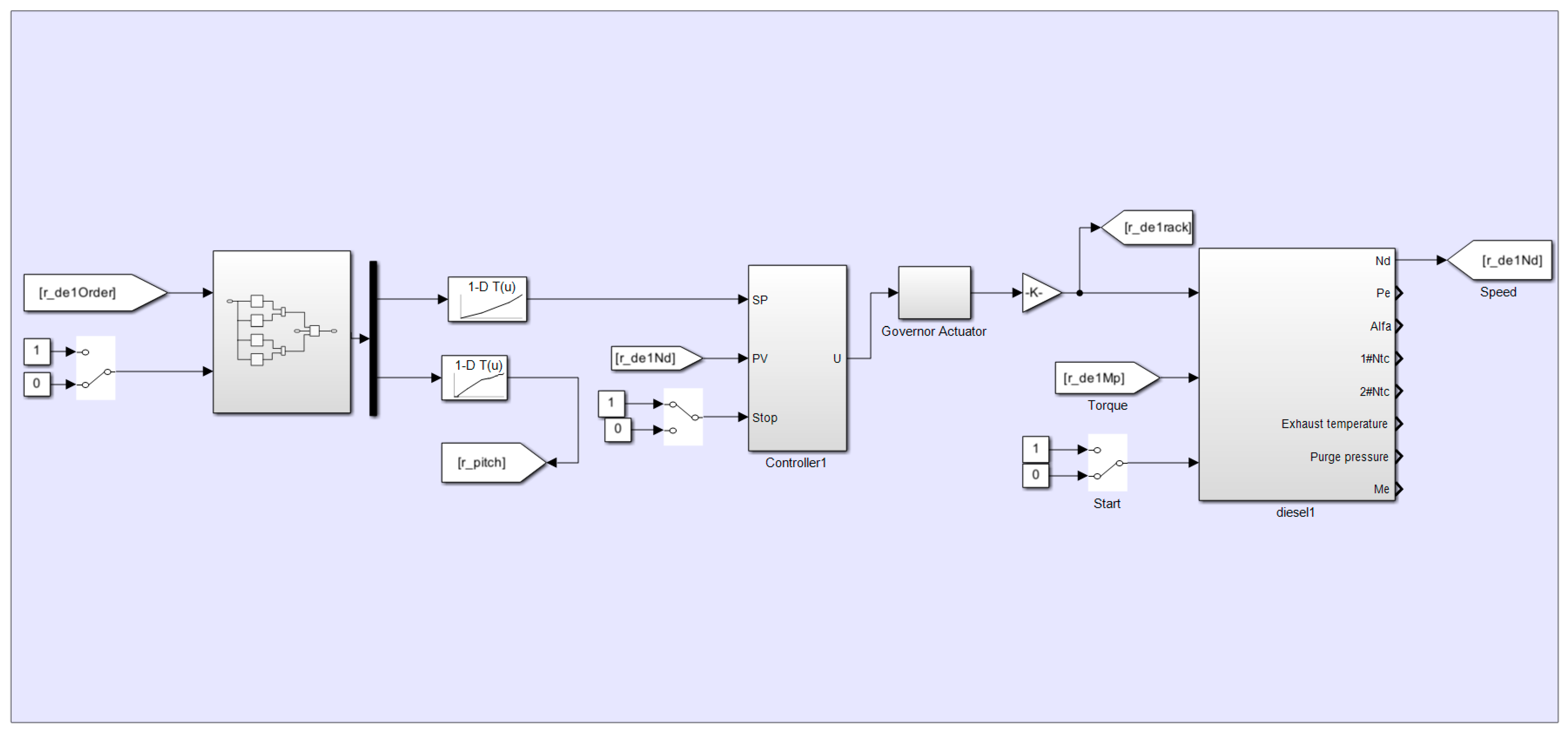
By interfacing the above sub-models and coupling their parameters, the complete simulation model of the diesel engine prime mover is constructed and encapsulated. Through real-time data exchange among the sub-models, the dynamic characteristics are simulated in a coupled manner. The diesel engine simulation model built in MATLAB/Simulink is shown in Figure 6. Detailed Simulink block diagrams of each sub-module are provided in the Supplementary Materials, Figures S1–S16.

Following the modular integration of the individual diesel engine sub-models, offline simulation validation is carried out based on MATLAB/Simulink. This validation is not intended to demonstrate absolute numerical agreement between the simulation model and the actual diesel engine—which depends on subsequent bench calibration experiments—but rather to verify the effectiveness at the following two levels from the perspective of control system development: (i) using the rotational speed dynamic response characteristics as the core evaluation metric, to verify whether the PID closed-loop speed controller enables the simulation model to accurately and rapidly track the target speed commands at different setpoints, thereby demonstrating the effectiveness of the control algorithm; and (ii) to verify whether the dynamic response trends of the simulation model conform to the general physical laws and engineering experience of diesel engines, thereby ensuring the fundamental credibility of the model as a controller development platform.

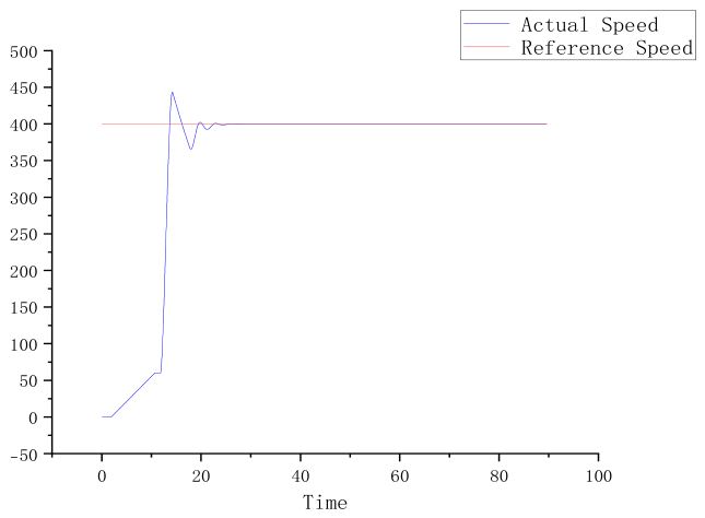
First, simulation validation under diesel engine startup conditions is conducted. Under zero initial load, a standard startup speed command is applied and the dynamic tracking process of the actual output speed relative to the theoretical reference speed is observed in real time, with key metrics such as the speed rise rate during the startup phase, steady-state settling time, and the peak overshoot being analyzed. Figure 7 illustrates the rotational speed evolution after engine startup, which can be divided into two phases: 0–60 rpm corresponds to the high-pressure air-turning phase, lasting approximately 10 s; and 60–400 rpm corresponds to the firing phase. After ignition, the speed rises to a peak of approximately 440 rpm, then drops to about 360 rpm, and finally stabilizes at 400 rpm after minor oscillations under the action of the PID controller. The maximum speed overshoot throughout the entire process is approximately 10%; the steady-state settling time is approximately 25 s. During the startup phase, because a sustained deviation exists between the actual speed and the target speed, the integral term of the PID controller continues to accumulate, producing a large fuel command. As the speed approaches the target value, the fuel command fails to decrease promptly due to the lag effect of the integral term, resulting in the fuel supply exceeding the steady-state demand, and, consequently, causing overshoot. Subsequently, as the error signal reverses, the controller gradually reduces the fuel command and the speed decreases and stabilizes.

The simulation results indicate that the speed overshoot is within the engineering allowable range (≤10%), the steady-state settling time is consistent with the typical dynamic response characteristics of large low-speed diesel engine startup processes, and the actual speed can quickly recover after overshoot and remain stable near the reference speed without sustained oscillation or divergence. These results demonstrate that the diesel engine prime mover model exhibits reasonable dynamic response characteristics, and that the governor PID closed-loop control logic is effective, applicable, and capable of meeting the basic requirements of an actual diesel engine startup operation.

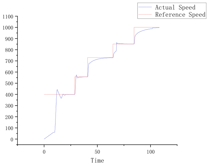
Simulation validation under multi-step speed command tracking conditions is then conducted. The control commands are sequentially increased from Level 1 to Level 5, simulating typical continuous speed-changing operations in actual practice. The deviation between the actual rotational speed and the corresponding reference speed at each command level is recorded in real time. By comparing the steady-state speed errors and the response delays during dynamic transitions at each steady operating point, the self-adaptive regulation capability of the model under variable-speed conditions is evaluated. 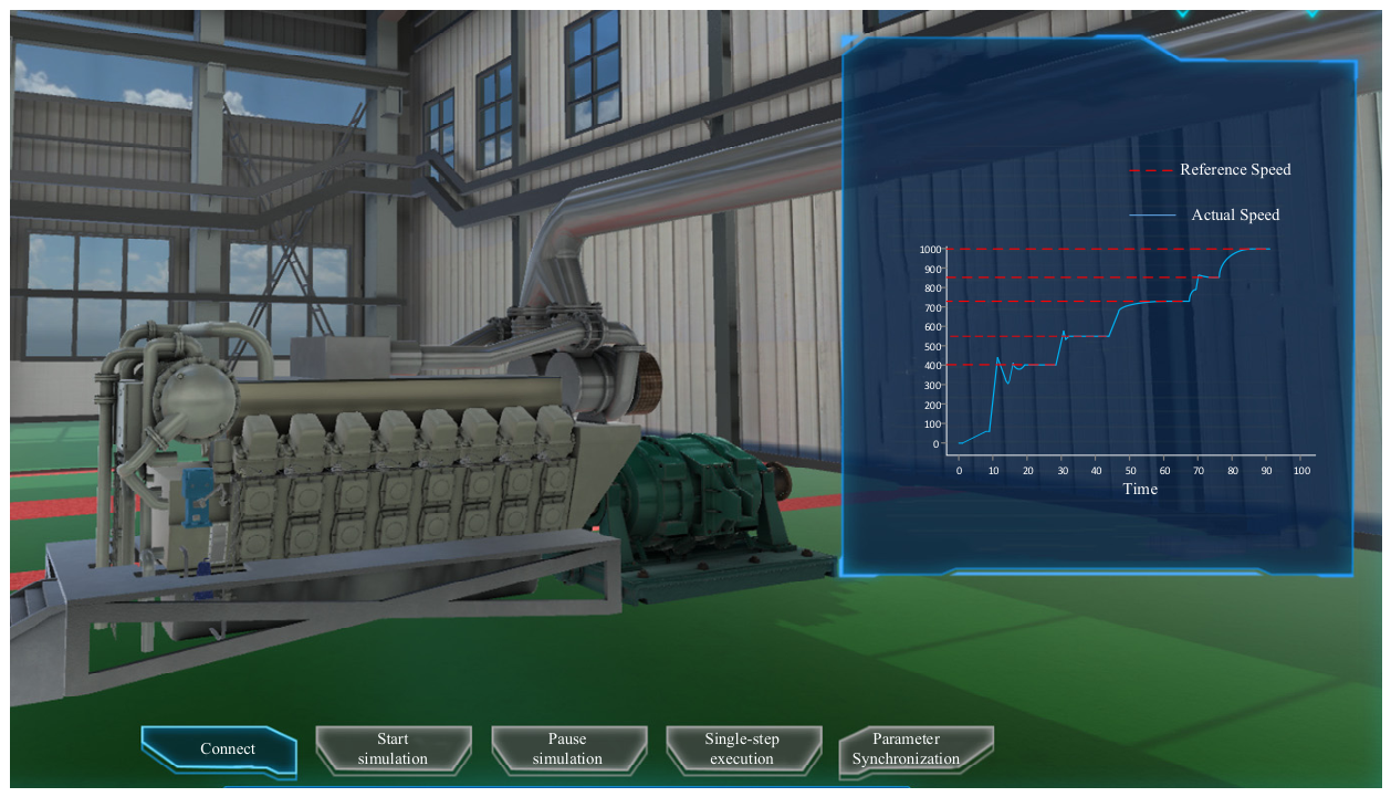Figure 8 illustrates the rotational speed evolution of the diesel engine under speed command changes. During 0–30 s, the speed response under Level 1 command is shown, which is consistent with the startup speed evolution described above. During 30–45 s, under Level 2 command, the reference speed is 556 rpm. The actual speed initially rises to a peak of about 580 rpm, then drops to approximately 540 rpm, and finally stabilizes at 556 rpm. The maximum overshoot throughout this phase is about 4.3% and the steady-state settling time is approximately 10 s. During 45–70 s, under Level 3 command with a reference speed of 730 rpm, the actual speed increases monotonically, always remaining below the reference, with no overshoot observed, and eventually stabilizes at 730 rpm under PID control, with a settling time of about 25 s. During 70–85 s, under Level 4 command, with a reference speed of 850 rpm, the actual speed first rises to a peak of approximately 866 rpm, then decreases and stabilizes at 850 rpm, with a settling time of about 15 s. During 85–105 s, under Level 5 command, with a reference speed of 1000 rpm, the actual speed increases monotonically, remains below the reference without overshoot, and finally stabilizes at 1000 rpm under PID control, with a settling time of about 20 s. The simulation results show that after each speed command, the actual speed can quickly track the target speed, with small dynamic deviations and fast steady-state convergence; no significant oscillations or control instability are observed under any condition. It should be highlighted that the zero steady-state error shown in

Table 3. Quantitative performance metrics for each command level in offline simulation.

Command Level	Time Interval (s)	Target Speed (rpm)	Steady-State Speed (rpm)	Steady-State Error (%)	Peak Speed (rpm)
Level 1	0–30	400	400	0	440
Level 2	30–45	556	556	0	580
Level 3	45–70	730	730	0	730
Level 4	70–85	850	850	0	866
Level 5	85–105	1000	1000	0	1000

originates from the integral action of the PID governor controller; it cannot be regarded as evidence for physical fidelity of the diesel engine plant model. Controller tracking performance and plant-model physical validation are strictly distinguished throughout this paper. Since there is no publicly available benchmark dataset fully matching our 2000 kW marine diesel engine, physical calibration is not performed at the current stage. In future work, we will adopt the self-calibrating digital-twin framework proposed by Zhang [20], which combines physics-based models and data-driven correction layers to reconcile simulation outputs with physical system behavior. The quantitative performance metrics for each command level in the offline simulation are summarized in Table 3.

Based on the simulation verification results of the two typical operating conditions, it can be concluded that the rotational speed response of the diesel engine simulation model exhibits qualitatively reasonable dynamic behavior consistent with general engineering expectations for diesel engine speed-control studies. This supports the use of the model as a preliminary platform for controller algorithm development but does not constitute validation of the model’s absolute predictive accuracy against a physical engine. The PID governor-based closed-loop control exhibits satisfactory regulation performance, with both dynamic errors and steady-state deviations maintained within reasonable ranges. The overall accuracy, stability, and dynamic adaptability of the model meet the application requirements for subsequent embedded code generation and embedded target deployment.

It is necessary to emphasize again that the verification presented in this section has the following attributes: (1) Controller-level verification: It mainly demonstrates that the closed-loop PID controller can track speed commands within the simulation environment. This reflects the effectiveness of the control algorithm, rather than the absolute accuracy of the plant model; (2) Qualitative rationality verification: The dynamic response trends of the model (startup characteristics, overshoot magnitude, settling time range) conform to the general physical laws of diesel engines, making the model suitable for use as a controller development platform; (3) Quantitative accuracy pending verification: The quantitative accuracy between the model and a real engine has not yet been validated. Even if the closed-loop system achieves zero steady-state error, this does not imply that the underlying open-loop model matches a physical engine—quantitative calibration via bench tests will be addressed in future work; and (4) Load disturbance testing: The multi-step command test is a speed-reference tracking test, not a true variable-load or load-disturbance test. No explicit load torque profile, propeller load law, generator-load disturbance, or measured duty-cycle profile is introduced in the current tests. Therefore, the results do not demonstrate the model’s behavior under real load-varying conditions.

4.4. Discussion on the Absence of Thermal Management Sub-Models

The current diesel engine simulation model focuses on governor, turbocharger, and prime-mover dynamic behavior, while thermal management subsystems, including cooling circuit, exhaust-manifold temperature dynamics, and intercooler thermal transients are not implemented. Therefore, the validity envelope of this simulation is restricted to speed control-oriented research only. This model cannot support the assessment of combustion efficiency, exhaust thermal load, and engine thermal-aging performance. Benefiting from our measured average CPU utilization of 14.2%, there remains considerable computational margin. Our modular six-layer software architecture theoretically supports the integration of thermal sub-models, referring to the thermal management methodology reported by Qiu [28], which employs field-synergy analysis for enhanced convective heat dissipation. Nevertheless, additional computational overhead brought by thermal dynamics needs to be carefully assessed before practical deployment. Thermal sub-model development is reserved for future iterations.

5. On-Target Embedded Simulation Testing

5.1. Online Simulation Test

To verify the operational reliability, real-time performance, and functional integrity of the embedded simulation software, a hardware online operation test is conducted based on the validated diesel engine simulation model. For code generation in this paper, MATLAB Embedded Coder R2022b is adopted. The target hardware is ARM Cortex-M4 (STM32F407VE), the compiler is ARM Compiler 6, and the simulation step size is set to 10 ms. The diesel engine model is converted into embedded C code targeting the STM32F407VE main controller via the Embedded Coder code generation tool, followed by code integration, project compilation, and firmware downloading, so that the simulation model can run independently online on the hardware platform. It should be noted that this system adopts a processor-in-the-loop (PIL) target-deployed simulation approach. Both the plant mathematical model and control logic execute on the same STM32 microcontroller, which is different than the classic test architecture, where a real physical ECU interacts with a separate virtual plant model. The system relies on the FreeRTOS real-time operating system to manage multi-task scheduling, simultaneously performing simulation computation, signal acquisition and processing, and hardware resource allocation, thereby ensuring temporal consistency and stability of the simulation process. The system test architecture is shown in Figure 9.

During online operation, the embedded controller uploads the real-time diesel engine rotational speed simulation parameters to the host computer monitoring system via the Ethernet TCP communication protocol. The host computer performs data reception, real-time display, and plotting of the operation curves. To comprehensively evaluate the dynamic response performance of the software system, simulation tests under diesel engine startup conditions and speed command adjustment variable-speed conditions are carried out, respectively. The real-time rotational speed variation curves are recorded by the host computer to verify the speed response characteristics, operation stability, and control real-time performance of the system under different operating conditions. Figure 10 and Figure 11 show the real-time rotational speed operation curves acquired by the host computer during diesel engine startup and speed command adjustment, respectively.

It should be noted that the online tests in this study recorded only the diesel engine rotational speed as the core, controlled variable. Other physical quantities—such as fuel command, torque, turbocharger speed, and intake manifold pressure—were not systematically recorded or validated. This is because the online tests were primarily designed with closed-loop speed control as the core validation objective and the current Ethernet communication protocol only supports real-time uploading of rotational speed data, without reserved fields for transmitting other variables. Consequently, the online test results demonstrate successful speed tracking and host-side visualization, but they do not verify the internal thermodynamic or dynamic states of the embedded model. Online validation of these intermediate variables is one of the key directions for future work.

The test results demonstrate that the proposed embedded simulation and control system exhibits stable communication interaction and can operate reliably under typical operating conditions such as startup and multi-step command tracking. The quantitative performance metrics for each command level in the online simulation are summarized in

Table 4. Quantitative performance metrics for each command level in online simulation.

Command Level	Time Interval (s)	Target Speed (rpm)	Steady-State Speed (rpm)	Steady-State Error (%)	Peak Speed (rpm)
Level 1	0–30	400	400	0	434
Level 2	30–45	556	556	0	576
Level 3	45–70	730	730	0	730
Level 4	70–80	850	850	0	862
Level 5	80–100	1000	1000	0	1000

. This system can serve as a preliminary verification aid for early-stage controller algorithm development, providing a reference for subsequent hardware-in-the-loop testing.

Table 5. Rotational speed error statistics between offline simulation and online simulation.

Working Condition	Max Absolute Error (rpm)	Mean Absolute Error (rpm)	RMSE (rpm)
Engine startup	6	6	6
Multi-step speed tracking	6	2.8	3.7

summarizes the numerical discrepancy of rotational speed outputs between offline Simulink simulation and STM32 on-target online execution across multiple test scenarios. Maximum absolute error, mean absolute error, and root-mean-square error are quantified.

5.2. Real-Time Performance Evaluation

To quantitatively verify the real-time performance and communication reliability of the system, this section systematically tests and evaluates task execution time, CPU utilization, memory footprint, and Ethernet communication quality:

(1) Task execution time measurement

Task execution time is measured using the 32-bit cycle counter (CYCCNT) of the Data Watchpoint and Trace (DWT) module embedded in the STM32F407VE. The counter is driven by the core clock (168 MHz), incrementing by one for each clock cycle; therefore, the time resolution is 1/168 MHz ≈ 5.95 ns. At the entry of each task under test, the CYCCNT value is read and saved as the start timestamp; at the task exit, the CYCCNT is read again as the end timestamp. The difference between the two readings provides the number of clock cycles consumed during that execution, which is then divided by the core clock frequency to obtain the execution time. To obtain statistically meaningful results, each task is measured over 1000 consecutive execution cycles, and the minimum, mean, maximum, and standard deviation are recorded;

(2) CPU utilization measurement

CPU utilization is measured using the Run-Time Statistics feature built into FreeRTOS. This method accumulates the actual CPU time consumed by each task through a high-resolution hardware timer. Within a fixed observation window (set to 1000 ms in this paper), the ratio of the sum of CPU times of all tasks to the window duration provides the CPU utilization. The CPU time proportion of the idle task reflects the system margin;

(3) Task-switching jitter measurement

Task period jitter is obtained by measuring GPIO toggling signals with a logic analyzer. Each task toggles a GPIO pin at the beginning of its period and the logic analyzer records the time intervals between consecutive toggles. Over 1000 consecutive periods, the standard deviation of the interval durations is computed as the jitter metric;

(4) Ethernet communication latency and reliability measurement

Communication latency is measured using the round-trip time (RTT) method: the host computer sends a request frame with a timestamp, and, upon reception, the target board immediately returns the frame. The host computer calculates the round-trip time and halves it to obtain an approximation of the one-way communication latency. A total of 10,000 frames are sent continuously and the mean and maximum latencies, as well as the packet loss rate, are statistically recorded.

Under the above measurement conditions, the real-time performance metrics of the core tasks are summarized in

Table 6. Real-time performance metrics of core tasks.

Task Name	Priority	Period (ms)	Execution Time (μs)	Jitter (μs)	WCET (μs)
Simulation model computation	High	10	312.5	8.2	485.6
Signal acquisition and processing	High	10	68.3	3.1	112.4
Ethernet communication	Medium	20	156.7	12.5	328.9

and the overall system resource usage is summarized in

Table 7. Overall system resource usage.

Metric	Value	Measurement Method
CPU utilization (peak)	18.7%	FreeRTOS Run-Time Statistics
CPU utilization (average)	14.2%	FreeRTOS Run-Time Statistics
Idle task CPU	81.3%	FreeRTOS Run-Time Statistics
Code storage (Flash) occupancy	156.4 KB	Compiler output
Data storage (RAM) occupancy	48.6 KB	Compiler output
Simulation task stack usage (peak)	512 bytes	FreeRTOS uxTaskGetStackHighWaterMark()

.

The average execution time of the simulation model computation task is approximately 312.5 μs, with a worst-case execution time (WCET) of 485.6 μs, accounting for only 4.9% of its period (10 ms = 10,000 μs), indicating a sufficient timing margin. The average execution time of the signal acquisition and processing task is about 68.3 μs, with a WCET of 112.4 μs. The average execution time of the Ethernet communication task is approximately 156.7 μs, with a WCET of 328.9 μs. No task exhibited period timeout or deadline miss.

The standard deviation of task period jitter is within 15 μs for all tasks, indicating that the FreeRTOS preemptive scheduler operates stably, with smooth task switching, and that no significant scheduling delays or jitter amplification caused by resource contention are observed.

The above real-time performance test results demonstrate that the embedded simulation platform designed in this paper has sufficient real-time computational margin on the STM32F407VE hardware (CPU utilization < 20%, and the execution time of each task is far less than its corresponding period). Even in the worst-case scenario, where all tasks reach their peak execution times simultaneously, the total CPU demand within a single period is approximately 485.6 + 112.4 + 328.9 = 926.9 μs, which is far less than the 10 ms period constraint, indicating that the system is not at risk of overload.

6. Conclusions

This paper presented the deployment of a Simulink-derived diesel engine speed-control model onto an STM32F407VE platform. The model was executed within the measured timing margins and used for closed-loop speed tracking in a small set of simulated scenarios (startup and multi-step speed commands). The following conclusions are supported by the presented evidence:

(1)

The MDD workflow (Simulink → Embedded Coder → STM32) is feasible for deploying a single-engine diesel simulation model onto a low-cost STM32 platform, with automatic code generation significantly reducing manual programming effort;

(2)

The implemented tasks execute within their specified periods on the STM32F407VE hardware, with a measured WCET of 485.6 μs for the simulation model computation task and a CPU utilization of 14.2%, on average;

(3)

The closed-loop PID controller can track speed commands in the simulation environment with zero steady-state error under the tested scenarios.

The following conclusions are NOT supported by the current evidence and should not be inferred from this study:

The physical diesel engine model has been validated against a real engine (it has not; bench calibration and quantitative accuracy verification remain to be studied in future work).

The generated code is numerically equivalent to the original Simulink model.

The platform provides comprehensive controller verification equivalent to physical engine testing (it does not; the current evidence supports only preliminary algorithm testing in a simulated environment).

The model’s behavior under true variable-load or load-disturbance conditions has been validated (it has not; only speed-reference tracking tests were conducted).

It should be noted that this study complements our previous research on parallel dual-engine diesel power systems [1]. Reference [1] primarily investigated coordinated control of two engines under parallel architecture, whereas the present paper establishes a dedicated single-engine simulation framework and verifies speed-control performance under typical operating conditions, including single-engine startup, idle speed stabilization, and multi-step speed command tracking. The core value of this paper lies not in proposing novel theoretical methodologies, but in systematically integrating and validating a complete technical solution that applies the MDD workflow to the deployment of low-cost single diesel engine simulations. This solution covers model construction, automatic code generation, real-time task scheduling, and quantitative performance measurement. The proposed framework can serve as a reference paradigm for the development of similar embedded simulation platforms.

Meanwhile, several limitations of this study are explicitly acknowledged:

(1)

The diesel engine simulation model has not yet been calibrated or validated against real-engine dynamometer test data; the current validation only demonstrates the closed-loop command tracking capability of the PID controller and cannot substantiate the absolute accuracy of the model relative to the actual engine;

(2)

The real-time performance metrics reported in this paper are all measured on the STM32F407VE single hardware platform—these metrics would change if the hardware were replaced or more complex models were adopted;

(3)

The validation work has been primarily focused on speed-control performance. Online validation of intermediate variables—such as fuel command, torque, turbocharger speed, and intake manifold pressure—remains insufficient. Subsequent studies will complement the online measurement and comparative analysis of these variables;

(4)

The present model is constructed based on steady-state characteristic maps. During transient processes, actual operating conditions may temporarily exceed the range of calibrated data, under which circumstances the model’s accuracy cannot be guaranteed;

(5)

The control algorithm adopted in this paper is limited to the PID controller. The adaptability of the system to advanced control algorithms, such as fuzzy logic, sliding-mode control and model predictive control, has not been verified. Although the controller module can be replaced via standardized interfaces from an architectural perspective, differences in computational-resource requirements among various control algorithms may exceed the real-time computing capability of the current STM32F407VE hardware.

Future work will focus on the following directions:

(1)

completing model calibration and validation using real diesel engine dynamometer test data;

(2)

porting the entire simulation framework to higher-performance hardware platforms to support the high-precision, smaller step-size simulation of more complex models.

Despite the above limitations, the proposed approach demonstrates the feasibility and practical value of applying model-driven development to embedded diesel engine simulation, providing a useful reference for subsequent controller algorithm validation and embedded simulation platform development.