Article

Adaptive Multi-Objective Beamforming and Power Allocation for MIMO-ISAC in Low-Altitude Wireless Networks


by
Bing Yang
1,
Yan Huo
1,*,
Xin Fan
2 and
Chang Wang
3
1
School of Electronics and Information Engineering, Beijing Jiaotong University, Beijing 100044, China
2
School of Information Science and Technology, Beijing Forestry University, Beijing 100083, China
3
Economic and Technological Research Institute, State Grid Jibei Electric Power Company Limited, Beijing 100053, China
*
Author to whom correspondence should be addressed.
Electronics 2026, 15(18), 4121; https://doi.org/10.3390/electronics15184121
Submission received: 14 August 2026 / Revised: 4 September 2026 / Accepted: 8 September 2026 / Published: 11 September 2026
(This article belongs to the Special Issue Communication Systems in Unmanned Aerial Vehicles)

Abstract

Low-altitude wireless networks (LAWNs) require reliable multi-user communication together with accurate range and velocity sensing. Communication and sensing share the same transmit power and spatial degrees of freedom (DoF), and therefore joint beamforming is required to coordinate multi-user spectral efficiency with delay-Doppler estimation accuracy. An adaptive multi-objective beamforming and power allocation framework is developed for a multiple-input multiple-output (MIMO) integrated sensing and communication (ISAC) base station. Communication performance is measured by the achievable multi-user sum spectral efficiency. Sensing performance is characterized by the Cramér–Rao lower bounds (CRLBs) for delay and Doppler frequency. A dimensionless system effectiveness integrated metric (SEIM) combines the three normalized performance components. The beamforming problem is lifted to transmit covariance matrices and treated via semidefinite relaxation (SDR) and alternating successive convex approximation (SCA) under power and per-user signal-to-interference-plus-noise ratio (SINR) constraints. An entropy-regularized weight subproblem provides a closed-form softmax update, and a damping step couples the weight update with the covariance iterations. Numerical results characterize the communication–sensing tradeoff with respect to the transmit power, array size, user loading, SINR requirements, and objective weights.

1. Introduction

Integrated sensing and communication (ISAC) has emerged as a pivotal enabler for sixth-generation (6G) networks by supporting communication and sensing (C&S) through common radio resources [1,2]. Low-altitude applications such as unmanned aerial vehicle (UAV) logistics and urban air mobility impose stringent requirements on both functions. Shared hardware and common spectral bands improve spectral utilization and reduce hardware duplication relative to separate C&S platforms [3,4,5]. Multiple-input multiple-output (MIMO) processing further provides spatial multiplexing for multi-user transmission and spatial diversity for sensing parameter estimation [6]. These capabilities support high-resolution sensing, obstacle avoidance, and reliable low-latency links in bandwidth-constrained low-altitude networks [7,8].
Joint MIMO-ISAC design must reconcile different waveform structures and performance measures [9]. Frequency-modulated continuous-wave (FMCW) and phase-modulated continuous-wave (PMCW) radar waveforms use deterministic signal structures that support coherent integration and matched-filter parameter estimation. Their restricted data modulation limits communication spectral efficiency [10]. Communication waveforms such as orthogonal frequency-division multiplexing (OFDM) and filter bank multicarrier (FBMC) provide flexible data modulation, while their sensing performance depends on the transmitted symbol realization and the associated time–frequency moments. The range and velocity accuracy are governed by effective bandwidth and coherent observation duration, respectively [11]. Communication performance is commonly described by the spectral efficiency or bit error rate, whereas sensing performance is described by the beampattern error or parameter estimation bounds [12,13]. A joint design must therefore combine quantities with different dimensions and optimization directions. Weighted multi-objective formulations provide a scalar representation of the communication-sensing (C-S) tradeoff, but fixed weights select only one operating preference and can be sensitive to the numerical scales of the constituent metrics [14]. Boundary-based normalization establishes comparable dimensionless components, and adaptive weight selection allows the scalarization to respond to the performance delivered by the current beamformers. The resulting covariance design remains nonconvex because the multi-user rates couple all communication and radar beams through interference, while delay and Doppler information depend on the same transmit covariances. Practical operation additionally requires an iterative method with controlled computational cost [15,16].
Table 1 summarizes representative waveform and resource co-design methods. Beampattern-matching methods align the transmit covariance with a desired sensing covariance while imposing communication signal-to-interference-plus-noise ratio (SINR) constraints. Dong et al. [12] solved the resulting design through iterative convex relaxation. Such formulations directly control spatial radiation but do not explicitly optimize delay or Doppler estimation accuracy. Cramér–Rao lower bound (CRLB) based methods instead connect the covariance design to parameter estimation information. Liu et al. [13] minimized a CRLB matrix trace under power and SINR constraints by exploiting the eigenspace of composite channel matrices. The resulting design depends on the rank and conditioning of the target response model, which motivates regularized or prior-aided formulations for uncertain sensing channels [6,17].
Reconfigurable intelligent surfaces (RISs) extend ISAC coverage by creating controllable indirect propagation paths. Zhu et al. [18] jointly configured the reflecting phases for non-line-of-sight (NLoS) sensing, with performance determined by the accuracy of the cascaded channel information. Other formulations separate or augment the available resources. Subcarrier allocation partitions sensing and communication functions in the frequency [15]. Bayesian localization incorporates prior target information through the posterior CRLB [17]. Sensing-assisted physical-layer security uses direction-of-arrival estimates to shape confidential beams and suppress leakage toward potential eavesdroppers [19]. These methods address specific propagation or service requirements. Accordingly, the considered low-altitude system jointly optimizes multi-user communication performance and delay–Doppler estimation accuracy under a common power budget.
Three coupled issues motivated the proposed design. First, weighted multi-objective waveform design requires a priori specification of the objective preferences, and different weights lead to different C-S operating points [14]. Second, practical constraints in joint MIMO radar–communication waveform design increase the complexity of the resulting optimization problem [20]. Third, mobility leads to time-varying channel geometry and target kinematics, which motivates sensing-assisted predictive beamforming in mobile links [7]. Accordingly, each beam design interval is represented by a quasi-static channel snapshot, and the proposed design optimizes the communication-sensing beamformers using the current CSI and predicted target direction. The proposed formulation combines dimensionless performance normalization, alternating covariance optimization, and adaptive scalarization within one beam design interval.
The main contributions are summarized as follows:
  • We establish an MIMO-ISAC signal model for multi-user downlink transmission and target tracking. The target direction is supplied by a preceding acquisition stage and is treated as known during one beam design interval. Communication data and the radar probing signal are jointly transmitted, and both are exploited in delay–Doppler estimation.
  • A dimensionless metric, termed the system effectiveness integrated metric (SEIM), is defined as a weighted sum of normalized communication sum spectral efficiency, delay information, and Doppler information. The normalization boundaries are evaluated over the same power, SINR, and radar-resource feasible set as the joint problem.
  • The non-convex beamforming problem is lifted to transmit covariance variables and treated by semidefinite relaxation (SDR). An alternating successive convex approximation (SCA) procedure constructs convex lower-bound subproblems for the radar and communication covariance blocks while retaining the total power and per-user SINR constraints.
  • The objective weights are obtained from an entropy-regularized scalarization subproblem. Its closed-form softmax solution and a damping step produce a simplex-preserving adaptive update between covariance iterations.
The remainder of this paper is organized as follows. Section 2 presents the MIMO-ISAC system model and defines the communication and radar performance metrics. Section 3 proposes a weighted multi-objective optimization framework. Section 4 provides extensive simulation results and evaluates the performance. Finally, Section 5 concludes the work.

2. System Model, Communication and Sensing Metrics, and Problem Formulation

As illustrated in Figure 1, a colocated MIMO-ISAC base station employs N t transmit antennas and N r receive antennas to serve K single-antenna ground users and track one low-altitude UAV target. The considered deployment adopts a moderate-aperture far-field operating regime in which the communication users and the tracked UAV lie beyond the Fraunhofer distance of the array such that the planar-wave array-response model provides an appropriate approximation. The BS–UAV link is characterized by a relatively short slant range, LoS-dominated target propagation, and non-negligible target motion, and the target state relevant to the beamforming design is represented by its range, azimuth, and radial velocity, with the latter captured through the Doppler frequency. A preceding search stage provides the predicted target azimuth θ for the current beam design interval. The downlink channels are assumed to be quasi-static within each transmission block, all users share the same time–frequency resources, and perfect channel state information (CSI) is available at the base station. The communication subsystem is Multi-User Multiple-Input Single-Output (MU-MISO), whereas the complete transmit–receive sensing platform is MIMO-ISAC. This operating configuration is consistent with emerging IMT-2030 ISAC usage scenarios, where range, velocity, and angle estimation constitute representative sensing capabilities, as well as ongoing 3GPP studies on ISAC service requirements and NR-oriented sensing waveform, channel, and radio interface design.

2.1. Signal Model

Communication and sensing share the carrier frequency f 0 , i.e.,  f com = f rad = f 0 , and all subsequent signals are complex baseband equivalents. The unit-power communication waveform for user k is
x k ( t ) = i s = 0 N s 1 b k , i s p t i ~ s T s , i ~ s = i s N s 1 2 , k = 1 , , K ,
where i s is the communication-symbol index, b k , i s is the corresponding zero-mean quadrature amplitude modulation (QAM) symbol for user k, p ( t ) is the pulse-shaping filter, T s is the symbol interval, and  N s is the number of symbols in one processing block. We assume that E { | x k ( t ) | 2 } = 1 and E { x k ( t ) x k * ( t ) } = 0 for k k . The block is centered at t = 0 , and  p ( t ) has an even energy envelope, as is the case for the truncated root-raised-cosine pulse used in the simulations.
The radar coherent processing interval (CPI) contains an equal-energy up/down linear frequency-modulated (LFM) pair. Its two normalized members are
s χ ( t ) = A LFM exp j π χ B LFM T p t 2 , s n , χ ( t ) = e j ϕ n s χ ( t ) , | t | T p / 2 , χ { 1 , + 1 } ,
where j = 1 denotes the imaginary unit, A LFM is selected to satisfy the unit average power, B LFM is the swept bandwidth, T p is the pulse duration, χ is the chirp-slope sign, and  ϕ n is the phase assigned to transmit antenna n, where n = 1 , , N t . Pairing the two slopes cancels out their opposite delay–Doppler cross-information while preserving their energy, effective bandwidth, and coherent duration. For the active slope, s ( t ) denotes the common waveform s χ ( t ) . The known factor e j ϕ n in s n , χ ( t ) is absorbed into w r , n in the subsequent baseband model.
Let w r = [ w r , 1 , , w r , N t ] T C N t be the radar beamforming vector, let w c , k = [ w c , 1 , k , , w c , N t , k ] T C N t be the beamformer for user k, and define W c = [ w c , 1 , , w c , K ] C N t × K . The joint signal radiated by antenna n is
s n joint ( t ) = w r , n s ( t ) + k = 1 K w c , n , k x k ( t ) .
Consequently, the radar and communication powers are P r = w r 2 2 and P c = W c F 2 = k w c , k 2 2 , respectively.
The implementation uses pulsed time-division duplexing (TDD) sensing [21,22]. The joint signal is transmitted in an active slot, followed by a silent echo-reception window in which radar and communication transmission are paused.

2.2. Multi-User Multiple-Input Single-Output Communication Subsystem

Let h c , k C N t denote the effective channel for the communication beams to user k. The communication channel follows a Rician model and is expressed as follows:
h c , k = β c , k K c , k K c , k + 1 h c , k LoS + 1 K c , k + 1 h c , k NLoS ,
where β c , k is the large-scale channel gain, K c , k 0 is the Rician factor, h c , k LoS is the deterministic line-of-sight (LoS) component, and  h c , k NLoS CN ( 0 , I N t ) is the non-line-of-sight (NLoS) component [23]. Let h r , k C N t denote the leakage channel of the radar component to that user. The two vectors coincide when the components propagate through the same radio-frequency (RF) chain and carrier channel. Separate vectors support distinct effective channels after analog processing. During an active slot, user k receives
y k ( t ) = h c , k H w c , k x k ( t ) + i u k h c , k H w c , i u x i u ( t ) + h r , k H w r s ( t ) + z k ( t ) ,
where i u is the interfering-user index, the normalized radar stream s ( t ) was defined in Section 2.1, and  z k ( t ) CN ( 0 , σ c , k 2 ) . Treating interference as noise gives the unique user SINR
γ k = | h c , k H w c , k | 2 i u k | h c , k H w c , i u | 2 + | h r , k H w r | 2 + σ c , k 2 .
Then, the achievable sum spectral efficiency is
C sum = k = 1 K log 2 ( 1 + γ k ) .

2.3. Multiple-Input Multiple-Output Radar Subsystem

The transmit and receive uniform linear arrays (ULAs) have inter-element spacing d. Their steering vectors are
a t ( θ ) = 1 , e j 2 π ( d f 0 / c 0 ) sin θ , , e j 2 π ( d f 0 / c 0 ) ( N t 1 ) sin θ T ,
a r ( θ ) = 1 , e j 2 π ( d f 0 / c 0 ) sin θ , , e j 2 π ( d f 0 / c 0 ) ( N r 1 ) sin θ T ,
where c 0 is the propagation speed. For the monostatic link, r tar is the one-way target range, and v r is the radial velocity. The delay and Doppler frequency are τ = 2 r tar / c 0 and f D = 2 v r f 0 / c 0 , respectively. The complex reflection coefficient α follows a Swerling-I model. It is constant within one coherent processing interval (CPI), independent between CPIs, and satisfies
E { | α | 2 } = G t G r c 0 2 σ ¯ ( 4 π ) 3 f 0 2 r tar 4 ,
where G t and G r are hardware antenna gains and σ ¯ is the mean radar cross-section. The received echo power therefore follows the two-way r tar 4 propagation law. The coefficient can be written as α = | α | e j ψ , where the reflection phase ψ U ( 0 , 2 π ) is constant within the CPI.
The transmitted signal vector is
x joint ( t ) = [ s 1 joint ( t ) , , s N t joint ( t ) ] T .
Furthermore, the continuous-time radar return is
y r ( t ) = α a r ( θ ) a t H ( θ ) x joint ( t τ ) e j 2 π f D t + z r ( t ) ,
where z r ( t ) is spatially white noise with a variance σ r 2 per receive antenna. Let T samp denote the radar sampling interval, and let N be the number of samples in one CPI. For the sample index { 0 , , N 1 } , the noise-free mean at t = T samp is
μ [ , ν ] = α a r ( θ ) a t H ( θ ) x joint ( T samp τ ) e j 2 π f D T samp ,
where ν = [ τ , f D ] T is the delay–Doppler parameter vector. The sampled return is
y r [ ] = μ [ , ν ] + z r [ ] .
where x joint ( T samp τ ) is a fractional-delay waveform. The continuous-delay mean is differentiable with respect to τ and supports the Fisher information matrix (FIM) construction below.
Conditioned on the known transmitted waveform, the mean μ [ , ν ] C N r in Equation (14) yields the FIM
[ J ( ν ) ] a , b = 2 σ r 2 = 0 N 1 μ H [ ] ν a μ [ ] ν b ,
where a , b { 1 , 2 } , ν 1 = τ , and  ν 2 = f D . For the unbiased estimator ν ^ = [ τ ^ , f ^ D ] T , we have
Cov ( ν ^ ) J 1 ( ν )
according to [24,25].
For a waveform component u q ( t ) , set u r ( t ) = s ( t ) for the radar pulse and u c , k ( t ) = x k ( t ) for user k’s communication waveform. The component index belongs to q { r , ( c , 1 ) , , ( c , K ) } . We then define
E q = | u q ( t ) | 2 d t , B q 2 = ( f f ¯ q ) 2 | U q ( f ) | 2 d f E q , T q 2 = ( t t ¯ q ) 2 | u q ( t ) | 2 d t E q ,
where f is the baseband frequency, U q ( f ) is the Fourier transform of u q ( t ) , and  f ¯ q and t ¯ q are its energy centroids. Thus, E r , B r , T r characterize the radar component, while E c , k , B c , k , T c , k characterize communication component k.
Let μ q ( t ) denote component q’s contribution to the noise-free mean, with the Doppler phase referenced to its energy centroid. Differentiation gives
μ q ( t ) τ = α a r ( θ ) a t H ( θ ) w q u ˙ q ( t τ ) e j 2 π f D t , μ q ( t ) f D = j 2 π ( t t ¯ q ) α a r ( θ ) a t H ( θ ) w q u q ( t τ ) e j 2 π f D t ,
where the overdot denotes differentiation with respect to time, w q = w r for q = r , and w q = w c , k for q = ( c , k ) . Parseval’s identity and Equation (17) yield
| u ˙ q ( t ) | 2 d t = 4 π 2 E q B q 2 , ( t t ¯ q ) 2 | u q ( t ) | 2 d t = E q T q 2 .
Theorem 1
(Conditional delay–Doppler decoupling). If the radar CPI contains the equal-energy up/down LFM pair defined above, and the centered communication blocks employ independent zero-mean symbols and an even-energy pulse, then the expected delay–Doppler cross-information J τ f D = [ J ( ν ) ] 1 , 2 satisfies E { J τ f D } = 0 . For an unpaired chirp or an asymmetric finite communication realization, the full 2 × 2 FIM in Equation (15) must be inverted.
Proof of Theorem 1.
See Appendix A.    □
Under the conditions of Theorem 1, the symbol-averaged delay–Doppler cross-information vanishes. Substitution of Equations (18) and (19) into Equation (15), followed by averaging over the mutually independent communication symbols, gives
J τ = κ E r B r 2 | a t H ( θ ) w r | 2 + k = 1 K E c , k B c , k 2 | a t H ( θ ) w c , k | 2 , J f D = κ E r T r 2 | a t H ( θ ) w r | 2 + k = 1 K E c , k T c , k 2 | a t H ( θ ) w c , k | 2 ,
where κ = 8 π 2 N r E { | α | 2 } / σ r 2 . The quadratic terms represent the transmit gain toward the predicted target angle θ , while N r accounts for coherent receive-array gain under the unnormalized steering-vector convention. The corresponding diagonal CRLBs are
CRLB τ = 1 J τ , CRLB f D = 1 J f D .
Thus, Equations (17)–(21) preserve the distinct roles of effective bandwidth and coherent duration.

2.4. Problem Formulation

A multi-objective formulation is adopted because communication and sensing impose simultaneous but potentially conflicting performance requirements on the shared transmit power and spatial degrees of freedom (DoF). Optimizing a single communication-oriented objective would generally favor multi-user transmission performance, whereas a sensing-oriented objective based solely on the estimation accuracy would tend to allocate more spatial resources toward target illumination. Such a single-objective design therefore cannot explicitly characterize the operating tradeoff among the communication rate and different sensing dimensions. This observation is consistent with the CRB-rate tradeoff and multi-objective communication–sensing formulations reported in [6,14,26]. Accordingly, the multi-objective framework adopted here provides a unified means of coordinating heterogeneous communication and sensing requirements within the same feasible set. Moreover, its normalized scalarization structure is not restricted to the three objectives considered in this work and can be extended to incorporate additional system-level criteria, such as energy efficiency, latency, reliability, or other sensing-quality measures, by introducing the corresponding normalized utilities and objective weights.
Specifically, the beamforming design simultaneously considers the communication sum spectral efficiency in Equation (7), the delay CRLB, and the Doppler CRLB in Equation (21). The communication quantity is maximized, whereas both CRLBs are minimized. Direct aggregation is inappropriate because the three quantities have different physical dimensions, numerical scales, and optimization directions.
The total power P all > 0 is divided by a prescribed power-partition parameter η ( 0 , 1 ) . Let γ th > 0 denote the required SINR of every user. During one beam design interval, the communication and radar allocations are
P c = η P all , P r = ( 1 η ) P all .
The power partition parameter η applies only to the division of the total transmit power between the communication and radar components during the active transmission slot and does not account for the subsequent silent echo reception window. Accordingly, the beamforming optimization and the communication spectral efficiency are defined for the active slot. When a frame-average communication metric is required, the resulting active-slot spectral efficiency is subsequently scaled by the communication duty factor determined by the fixed TDD frame structure.
The main algorithm optimizes the beamformers for a fixed η value, while the power partition experiment varies η . Thus, P c and P r are positive and remain unchanged when the three single-objective boundaries and the joint solution are computed for one operating point. The corresponding beamformer feasible set is
F = { ( w r , W c ) | W c F 2 = P c , w r 2 2 = P r , γ k γ th , k = 1 , , K } .
Let C max , J τ max , and  J f D max denote the communication, delay information, and Doppler information boundaries obtained from the single-objective problems in Section 3. The associated CRLB boundaries satisfy
CRLB τ min = 1 J τ max , CRLB f D min = 1 J f D max .
To this end, the normalized performance components are
U c = C sum C max , U τ = CRLB τ min CRLB τ = J τ J τ max , U f D = CRLB f D min CRLB f D = J f D J f D max .
Here, U c denotes the normalized communication utility, whereas U τ and U f D denote the normalized delay and Doppler information utilities, respectively. All three quantities are dimensionless, with larger values indicating better performance relative to their corresponding single-objective reference boundaries.
The two equivalent forms of each sensing component follow directly from Equations (21) and (24). Let λ = [ λ c , λ τ , λ f D ] T denote the objective-weight vector. The SEIM is
M SEIM = λ c U c + λ τ U τ + λ f D U f D .
The normalized C-S performance region associated with F is defined as follows:
R CS = { υ R + 3 | ( w r , W c ) F : 0 υ c U c ( w r , W c ) , 0 υ τ U τ ( w r , W c ) , 0 υ f D U f D ( w r , W c ) } ,
where υ = [ υ c , υ τ , υ f D ] T is an attainable normalized performance triple. A point belongs to the Pareto boundary of R CS if no other attainable point improves one component without decreasing at least one of the remaining components. Such performance-region descriptions have been used to characterize rate–CRB and multi-dimensional C–S tradeoffs in MIMO-ISAC systems [6,26].
The weight vector is selected from the probability simplex
Δ 3 = λ R + 3 | λ c + λ τ + λ f D = 1 .
Since explicitly characterizing the complete Pareto boundary of R C S is computationally prohibitive for the considered non-convex beamforming problem, this paper adopts the weighted-sum scalarization to efficiently obtain supported Pareto-optimal operating points.
For a prescribed λ Δ 3 , maximizing the SEIM selects a supported operating point of R CS . Strictly positive weights yield a Pareto-optimal global solution. The region definition and the scalarization serve different purposes; R CS describes the attainable tradeoff, while Equation (29) computes one operating point required by the proposed design.
For the prescribed weight vector, the normalized beamforming problem is
maximize w r , W c λ c C sum C max + λ τ J τ J τ max + λ f D J f D J f D max
subject to W c F 2 = P c
w r 2 2 = P r
γ k γ th , k = 1 , , K
P c + P r = P all .
The power and SINR constraints in Equations (29a)–(29d) impose the physical restrictions used in every boundary and joint-design instance. Section 3 expresses these restrictions in the covariance domain, applies SDR, determines the three boundaries once, and then solves Equation (29) by alternating covariance updates.

3. Problem Solution Framework

The problem in Equation (29) uses three normalization constants that are evaluated before the joint iterations. Each constant is obtained by selecting one performance quantity as the sole objective while retaining the common power, SINR, channel, and radar interference model. The resulting constants remain fixed during the subsequent covariance and weight updates.

3.1. Performance Boundary Determination

We define the transmit covariance matrices and the effective channel matrices as follows:
R r = w r w r H , R c , k = w c , k w c , k H , H c , k = h c , k h c , k H , H r , k = h r , k h r , k H .
In this case, the desired communication power and the interference-plus-noise power of user k are
S k = Tr ( H c , k R c , k ) , I k = i u k Tr ( H c , k R c , i u ) + Tr ( H r , k R r ) + σ c , k 2 .
Consequently, γ k = S k / I k , and the user constraint becomes
S k γ th I k , k = 1 , , K .
The matrix A θ = a t ( θ ) a t H ( θ ) describes the transmit direction of the tracked target. The information measures in Equation (20) have the covariance forms
J τ = κ E r B r 2 Tr ( A θ R r ) + k E c , k B c , k 2 Tr ( A θ R c , k ) , J f D = κ E r T r 2 Tr ( A θ R r ) + k E c , k T c , k 2 Tr ( A θ R c , k ) .
The covariance matrices in Equation (30) satisfy rank-one constraints. SDR removes these nonconvex constraints and retains positive semidefiniteness. Let ζ { C , τ , f D } identify the communication, delay information, and Doppler information boundary instances, respectively. The three instances are represented by the parameterized problem
maximize R r , { R c , k } C sum , ζ = C , J τ , ζ = τ , J f D , ζ = f D
subject to Tr ( R r ) = P r
k = 1 K Tr ( R c , k ) = P c
S k γ th I k , k = 1 , , K
R r 0
R c , k 0 , k = 1 , , K
P c + P r = P all .
The three instances of Equation (34) share the same P c , P r , P all , γ th , user channels, radar leakage channels, and PSD relaxation. The radar covariance remains active in the communication instance, and the user SINR constraints remain active in both sensing instances. Let ( R r ζ , , { R c , k ζ , } k = 1 K ) denote the covariance solution returned by instance ζ .

3.1.1. Cramér–Rao Lower Bound Minimization

Setting ζ = τ in Equation (34) maximizes J τ , while setting ζ = f D maximizes J f D . Both objectives in Equation (33) are affine in the covariance matrices, and all constraints in Equations (34a)–(34f) are affine or semidefinite. The two sensing instances are therefore standard SDPs after the rank relaxation. Their solutions define
J τ max = J τ R r τ , , { R c , k τ , } k = 1 K , J f D max = J f D R r f D , , { R c , k f D , } k = 1 K , CRLB τ min = 1 J τ max , CRLB f D min = 1 J f D max .
The two SDPs are solved separately because the effective bandwidth and coherent duration weight the waveform components differently. The coefficient sets { E q B q 2 } and { E q T q 2 } are generally not proportional across the radar and communication components. A waveform component can provide a large effective bandwidth and a short coherent duration or the opposite combination. Hence, the covariance that maximizes delay information need not maximize Doppler information.

3.1.2. Communication Efficiency Maximization

The communication boundary follows from the ζ = C instance of Equation (34). For fixed covariance matrices, the contribution of user k can be written as follows:
C k = log 2 ( S k + I k ) log 2 ( I k ) ,
where C sum = k = 1 K C k . The difference of logarithms is not jointly concave in the covariance variables. Let m denote the SCA iteration index, and let I k ( m ) be I k evaluated at the current covariance point. The concavity of log 2 ( I k ) gives the lower approximation
C ^ k ( m ) = log 2 ( S k + I k ) log 2 ( I k ( m ) ) I k I k ( m ) I k ( m ) ln 2 .
The approximation is tight and gradient-consistent at the current covariance point. Replacing C k with C ^ k ( m ) yields a convex program with semidefinite constraints at each SCA iteration. The converged communication value is
C max = C sum R r C , , { R c , k C , } k = 1 K .
Throughout the paper, C max denotes the value returned by this single-objective SDR–SCA boundary calculation. The radar power, radar interference, and user SINR requirements are identical to those used in the joint design. The three values in Equations (35) and (38) are evaluated once for an operating point and are used by every subsequent iteration and comparison method.

3.2. Waveform Optimization Design via Alternative Method

Substitution of Equation (33) into Equation (29) yields the relaxed normalized problem
maximize R r , { R c , k } λ c C max C sum + λ τ J τ max J τ + λ f D J f D max J f D
subject to Tr ( R r ) = P r
k = 1 K Tr ( R c , k ) = P c
S k γ th I k , k = 1 , , K
R r 0
R c , k 0 , k = 1 , , K
P c + P r = P all .
The normalization constants in Equation (39) remain fixed at the values obtained from Equation (34). The sensing terms are affine in the covariance matrices, whereas the sum spectral efficiency couples the radar and communication covariances through I k . Alternating SCA updates resolve this coupling.

3.2.1. Radar Covariance Update

Fix { R c , k } . The desired power S k is then constant, while the radar covariance affects the communication term through
I k ( R r ) = I 0 , k + Tr ( H r , k R r ) ,
where
I 0 , k = i u k Tr ( H c , k R c , i u ) + σ c , k 2 .
For ι > 0 , define φ k ( ι ) = log 2 ( 1 + S k / ι ) . Since φ k ( ι ) is convex, its first-order expansion at I k ( m ) = I k ( R r ( m ) ) gives the global lower bound
C ^ k , r ( m ) ( R r ) = φ k ( I k ( m ) ) + φ ˙ k ( m ) [ I k ( R r ) I k ( m ) ] ,
where
φ ˙ k ( m ) = 1 ln 2 1 I k ( m ) + S k 1 I k ( m ) < 0 .
And then, replacing C sum with k C ^ k , r ( m ) in Equation (39) gives an SDP in R r . The radar covariance update is summarized in Algorithm 1.
Algorithm 1 Radar covariance update via SCA
Input:         { R c , k } , { H c , k , H r , k } , λ , P r , γ th , and tolerance ϵ SCA .
1:
               Initialize a feasible R r ( 0 ) 0 .
2:
               repeat
3:
                  Evaluate I k ( m ) and φ ˙ k ( m ) for all k.
4:
                  Construct Equation (42) and solve the radar SDP using CVX 2.2 [27].
5:
                  Update R r ( m + 1 ) .
6:
               until the relative surrogate objective change is below ϵ SCA .
7:
               return  R r .

3.2.2. Communication Covariance Update

Fix R r , and evaluate I k ( m ) at the current communication covariances. Applying the difference-of-logarithms approximation to Equation (36) gives
C ^ k , c ( m ) = log 2 ( S k + I k ) log 2 ( I k ( m ) ) I k I k ( m ) I k ( m ) ln 2 .
The bound is concave in { R c , k } , is tight at the current iterate, and has the same first-order derivative as C k . Substituting k C ^ k , c ( m ) for C sum in Equation (39) yields a convex communication-covariance problem with semidefinite constraints. Algorithm 2 outlines the detailed procedure for the proposed scheme.
Algorithm 2 Communication covariance update via SCA
Input:         R r , { H c , k , H r , k } , λ , P c , γ th , and  ϵ SCA .
1:
               Initialize feasible { R c , k ( 0 ) 0 } .
2:
               repeat
3:
                  Evaluate I k ( m ) , and construct Equation (44).
4:
                  Solve the communication covariance SDP using CVX 2.2 [27].
5:
                  Update { R c , k ( m + 1 ) } .
6:
               until the relative surrogate-objective change is below ϵ SCA .
7:
               return  { R c , k } .

3.3. Multi-Objective Optimization with Adaptive Weight

After one radar and communication covariance cycle, collect the normalized components in
u ( m ) = [ U c ( m ) , U τ ( m ) , U f D ( m ) ] T .
The index set S w = { c , τ , f D } identifies the three entries of u ( m ) . The entropy-regularized scalarization score is
Ψ ( λ ; u ( m ) ) = λ T u ( m ) + 1 β w H ( λ ) ,
where β w > 0 controls the sensitivity of the weights and
H ( λ ) = ζ S w λ ζ ln λ ζ .
Maximizing Ψ over the simplex Δ 3 in Equation (28) gives the candidate
λ ~ ζ ( m ) = exp ( β w u ζ ( m ) ) ξ S w exp ( β w u ξ ( m ) ) , ζ S w .
The candidate is combined with the preceding weight vector through
λ ζ ( m + 1 ) = ( 1 ρ w ) λ ζ ( m ) + ρ w λ ~ ζ ( m ) , ζ S w ,
where ρ w ( 0 , 1 ] is the damping factor. A small β w value produces weights close to the uniform vector, whereas a larger value differentiates the three components more strongly. Equation (49) preserves the nonnegativity and unit sum and limits the change between consecutive scalarizations.
For a fixed λ value, the two SCA minorants are global lower bounds that are tight and gradient-consistent at the current covariance point. Exact solution of the two convex subproblems therefore produces a nondecreasing sequence of the fixed-weight objective in Equation (39). The feasible covariance set is compact under the power equalities, and thus the fixed-weight objective sequence converges. When Equation (49) is enabled, the scalarization changes between outer iterations. Convergence is then assessed from the covariance, normalized-component, and weight residuals stated in Algorithm 3.
Algorithm 3 Alternating SDR–SCA with adaptive weights
Input:         { H c , k , H r , k } , P c , P r , γ th , λ ( 0 ) , β w , ρ w , and tolerance ϵ out .
1:
               Solve the three instances of Equation (34), and store C max , J τ max , and  J f D max .
2:
               Initialize feasible R r ( 0 ) and { R c , k ( 0 ) } .
3:
               repeat
4:
                  Update R r ( m + 1 ) using Algorithm 1.
5:
                  Update { R c , k ( m + 1 ) } using Algorithm 2.
6:
                  Evaluate U c ( m + 1 ) , U τ ( m + 1 ) , and  U f D ( m + 1 ) using the stored boundaries.
7:
                  Compute Equation (48), and apply Equation (49).
8:
               until the relative covariance, utility, and weight changes are below ϵ out .
9:
               return  R r , { R c , k } , λ , and  M SEIM .
There are K + 1 Hermitian covariance blocks of a dimension N t . Their total number of real scalar variables is to the order of n v = ( K + 1 ) N t 2 , and the number of affine power and SINR constraints is to the order of n a = K + 2 . A dense primal-dual interior-point step has the arithmetic order O ( n v 3 + n a n v 2 + n a 2 n v ) . If I out , I SCA , and I IP denote the numbers of outer iterations, SCA iterations, and interior-point steps, respectively, then the two covariance updates require
O 2 I out I SCA I IP n v 3 + n a n v 2 + n a 2 n v .
The three exponentials and one normalization in Equation (48) have negligible costs relative to the SDP solutions.

3.4. Recovery of Transmit Beam Matrices

For a rank-one covariance solution, the beamforming vectors follow from the principal eigenpairs
w r = ϱ r , 1 e r , 1 , w c , k = ϱ c , k , 1 e c , k , 1 ,
where ( ϱ r , 1 , e r , 1 ) and ( ϱ c , k , 1 , e c , k , 1 ) are the largest eigenpairs of R r and R c , k , respectively. For any higher-rank covariance R returned by Equation (39), Gaussian randomization generates
w rnd = L z rnd , L L H = R , z rnd CN ( 0 , I N t ) .
where L is a matrix factor of R and I N t is the N t × N t identity matrix. Each candidate is rescaled to the prescribed communication or radar power and tested against the user SINR constraints. The feasible candidate with the largest value of Equation (26) is selected. The boundary values computed from Equation (34) remain the common normalization references for all recovered candidates and comparison methods.

4. Performance Evaluation

The numerical evaluation examines the spatial beam patterns, transmit power dependence, receive array size, user loading, SINR requirement, objective weights, power partition, and algorithmic benchmarks. The SEIM in Equation (26) is computed from boundary values obtained under the same parameter setting as the corresponding multi-objective point. Unless a horizontal-axis variable is changed, all parameters follow Table 2.

4.1. Network Set-Up

The nominal configuration employed 8 transmit and 8 receive antennas with half-wavelength spacing and served 4 single-antenna users, providing sufficient spatial DoF for simultaneous multi-user transmission and target-directed sensing while maintaining a manageable SDP dimension. A total transmit power of 10 W and an equal C&S power split with η = 0.5 were used as the nominal operating point, while P all was varied from 6 to 14 W in the power-dependent experiments. The minimum SINR threshold was set to 0.5 to impose a nonzero communication service requirement while retaining feasibility for the sensing-oriented designs. The nominal user distances and azimuths were [ 80 , 95 , 115 , 130 ] m and [ 50 , 15 , 20 , 55 ] , respectively, which provided heterogeneous propagation conditions and noncoincident spatial directions. For each channel realization, independent Gaussian perturbations were introduced as d k = d 0 , k ( 1 + ϵ d , k ) and ϑ k = ϑ 0 , k + δ ϑ , k , where ϵ d , k N ( 0 , 0.025 2 ) and δ ϑ , k N ( 0 , ( 2 ) 2 ) . The Rician factor was set to the linear value K c , k = 5 to represent LoS-dominated propagation with residual scattering. The tracked UAV is represented by a 100-m BS–UAV slant range and a predicted azimuth of 30 . Eight paired channel realizations were used for the algorithm comparisons, with the same realizations shared by all methods. The phase model ψ U ( 0 , 2 π ) refers specifically to the target reflection phase and not to the spatial distribution of the users or UAV. All numerical simulations were implemented in MATLAB R2021b, and the convex optimization problems were solved using CVX 2.2 [27].

4.2. Beampatterns at Boundary Operating Points

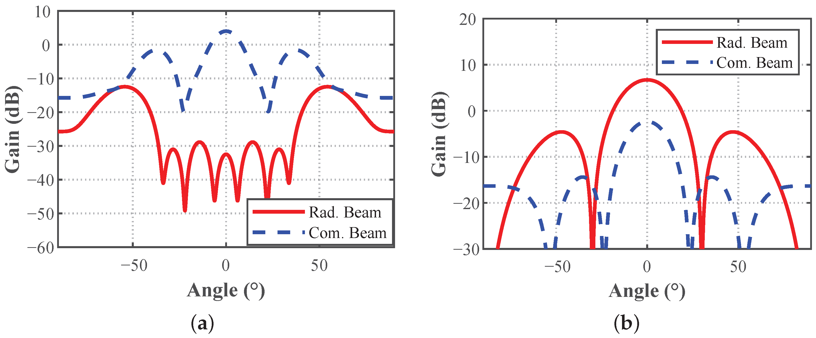
Figure 2 compares the transmit beampatterns at the communication and sensing boundaries. The red curve represents the radar beam, and the blue dashed curve represents the aggregate communication beam.
At the communication boundary in Figure 2a, the aggregate communication beam formed several angular peaks associated with the user directions. Its strongest lobe was located near the broadside, while additional peaks covered off-broadside users. The radar beam placed a deep attenuation region across the central user sector and redirected energy toward the outer angular regions. This spatial separation reduced radar leakage in the user SINRs while maintaining the prescribed radar power.
At the sensing boundary in Figure 2b, the radar beam formed its dominant mainlobe around the predicted target direction near the broadside. The communication beam maintained a lower-gain broadside lobe and off-axis components needed to satisfy the user SINR constraints. The contrast between the two panels shows how the same power allocation produced different covariance orientations. Communication-boundary optimization distributed energy among user directions, whereas sensing-boundary optimization increased the quadratic target-direction gains in Equation (20).

4.3. Impact of Transmit Power

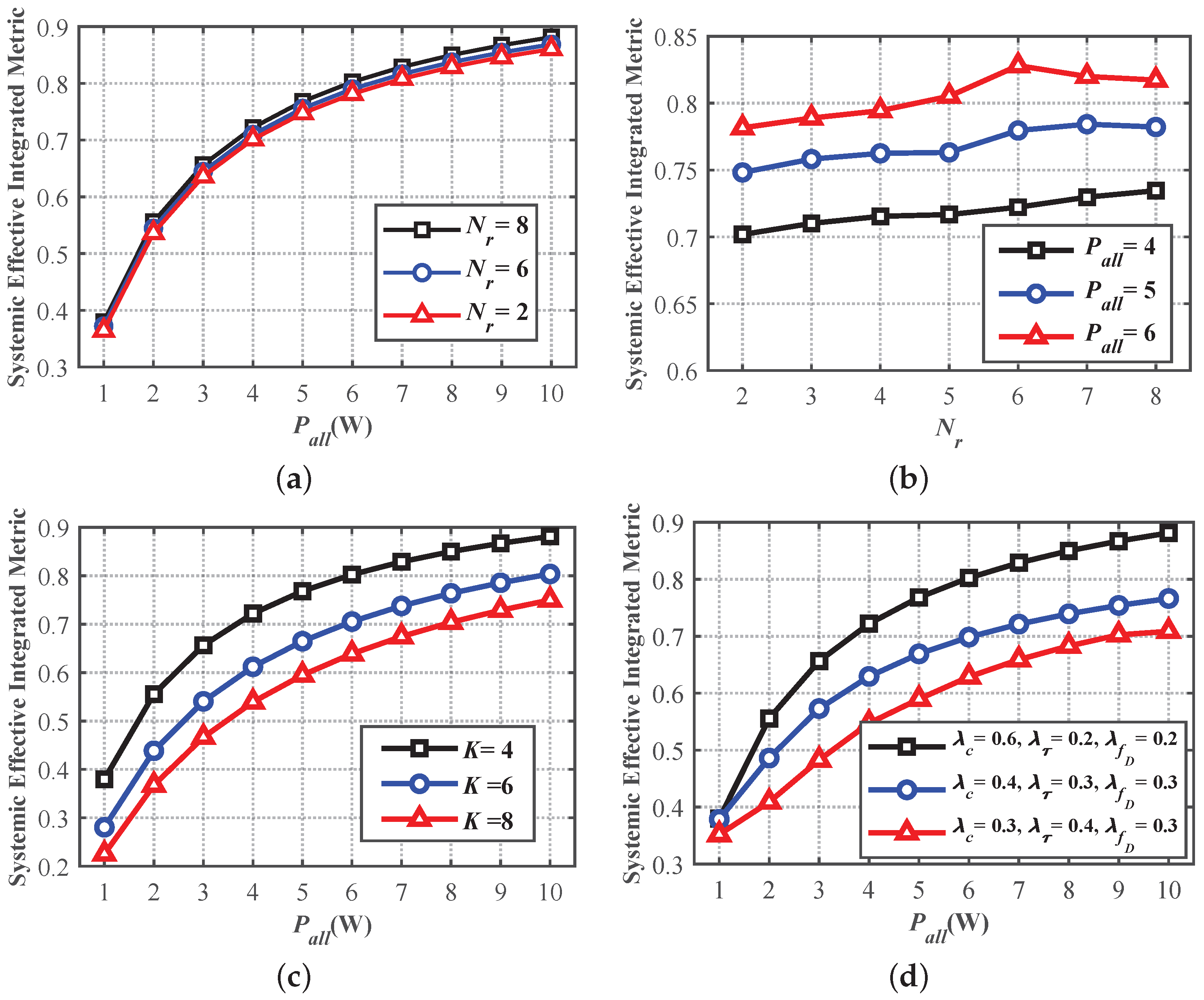
Figure 3a shows a monotonic SEIM increase as P all grew from 1 to 10 W. The increase was steep below approximately 4 W and became gradual at higher power levels. Additional transmit power first improved the noise-limited user SINRs and target illumination. Once these requirements were well supported, interference management and the normalization boundaries limited the incremental SEIM gain. The curves for N r = 2 , 6 , 8 remained close at low power and separated gradually as the power increased. A larger receive array increased the coherent echo gain through the factor N r in κ , which improved both the delay and Doppler information.
Figure 3b presents the complementary receive-array sweep. For each power level, the SEIM increased with N r , with small local variations caused by the joint covariance update. Raising P all from 4 to 6 W shifted the complete curve upward. The power increase produced a larger gain than adding receive antennas over the tested range, while the array increase provided a consistent sensing improvement without changing the communication-user count.
Figure 3c compares K = 4 , 6 , 8 . All curves increased with the transmit power, and the ordering remained K = 4 , K = 6 , and K = 8 from highest to lowest SEIM. Each additional user required an independent desired signal constraint and introduced further multi-user interference terms in Equation (6). The fixed transmit array must therefore allocate more spatial DoF to interference suppression, leaving less directional gain for the target.
Figure 3d evaluates three weight vectors. The setting ( λ c , λ τ , λ f D ) = ( 0.6 , 0.2 , 0.2 ) gave the largest SEIM throughout the tested power interval, followed by ( 0.4 , 0.3 , 0.3 ) and ( 0.3 , 0.4 , 0.3 ) . The separation widened with the power because the covariance optimizer had more freedom to realize the selected objective priority.

4.4. Impact of Communication Parameters

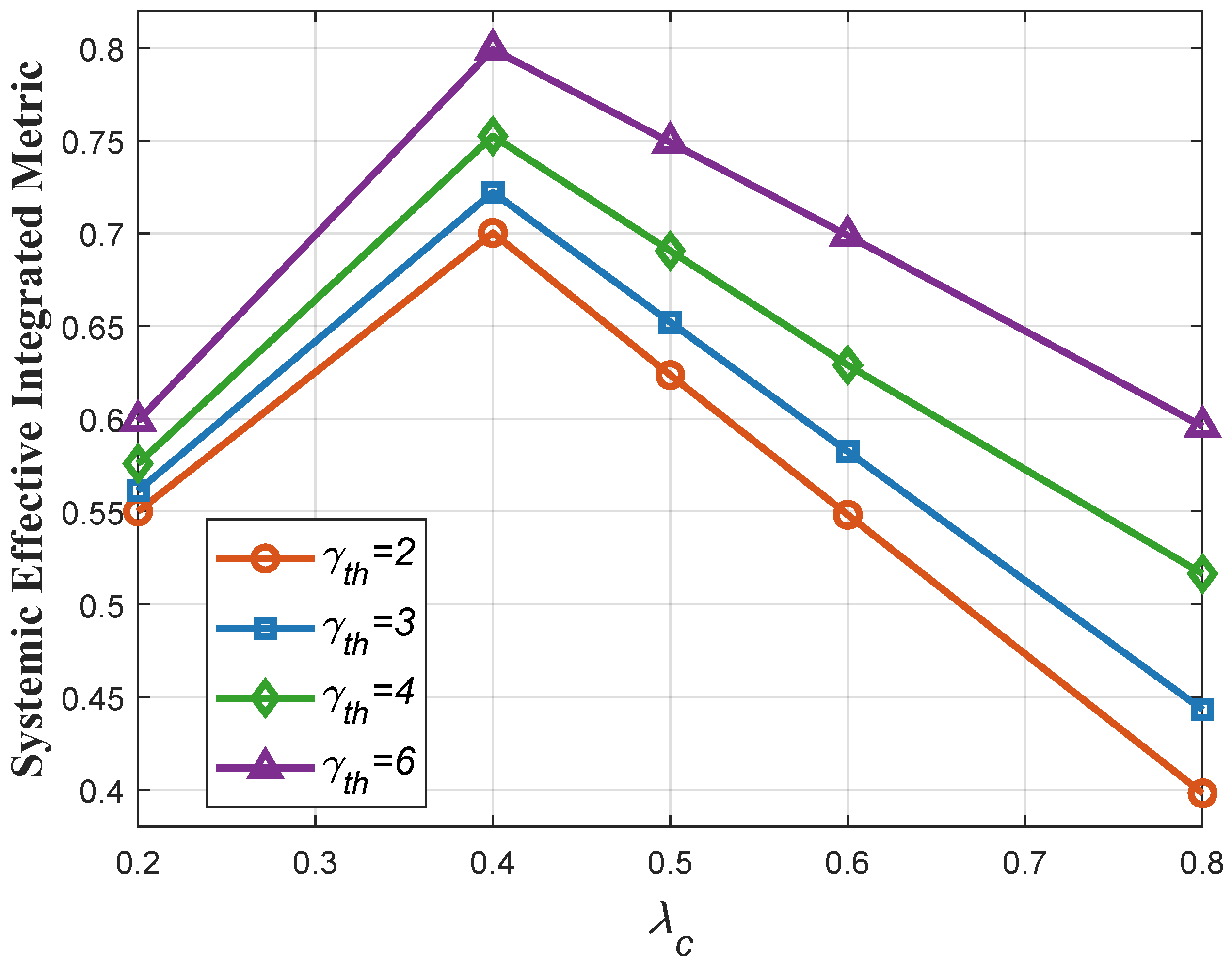
Figure 4 evaluates λ c { 0.2 , 0.4 , 0.5 , 0.6 , 0.8 } for four SINR thresholds. Every curve reached its maximum at λ c = 0.4 . Increasing λ c from 0.2 to 0.4 gave more emphasis to the communication component while preserving sufficient delay and Doppler weights. Beyond 0.4, the loss in the two sensing contributions exceeded the additional normalized communication gain, and the SEIM decreased. The decline was strongest for γ th = 2 , whose curve fell from approximately 0.70 at λ c = 0.4 to 0.40 at λ c = 0.8 .
The higher-threshold curves lie above the lower-threshold curves for the plotted normalized metric. The constraint in Equation (32) forced the covariance solution to maintain stronger desired signal terms as γ th increased. Under the boundary normalization associated with each threshold, this allocation raised the communication contribution to the SEIM and reduced the sensitivity of the curve to large λ c values. The common peak location indicates that λ c = 0.4 provided the most effective balance for the tested SINR range.
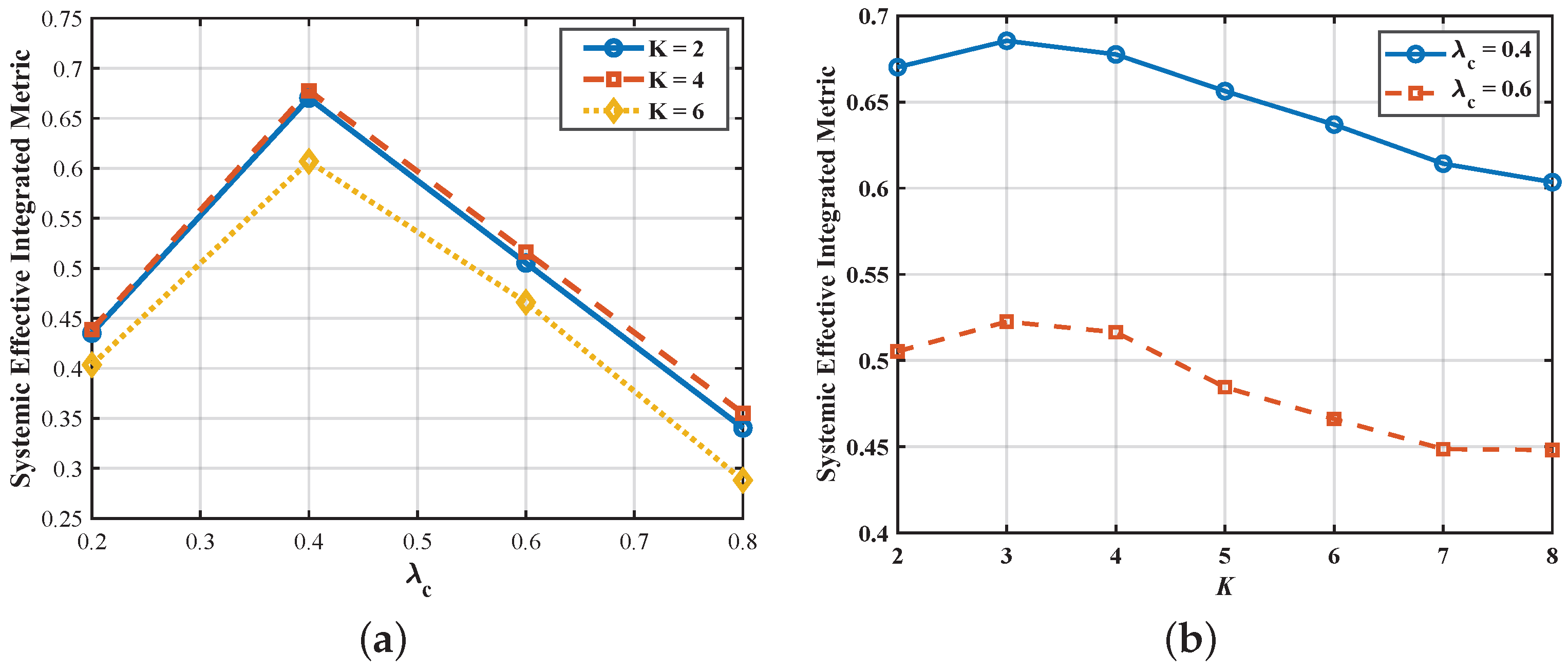
Figure 5a compares K = 2 , 4 , 6 over the same communication-weight grid. The three curves peaked at λ c = 0.4 , where the SEIM values were approximately 0.67, 0.68, and 0.61. The curves decreased rapidly when λ c rose from 0.4 to 0.8 because the combined weight assigned to delay and Doppler information became too small. The K = 6 curve remained below the two lighter-load curves, reflecting the additional spatial constraints imposed by six desired communication streams.
Figure 5b fixes λ c and varies the number of users from 2 to 8. For λ c = 0.4 , the SEIM reached a shallow maximum near K = 3 and then decreased from approximately 0.69 to 0.60. For λ c = 0.6 , the curve followed the same trend at a lower level and approached 0.45 for K = 7 and K = 8 . Moderate user loading initially added useful communication streams. Further loading increased the interference term I k for multiple users and consumed transmit dimensions that would otherwise increase Tr ( A θ R r ) and the sensing contribution of the communication covariances.

4.5. Comparison of Weighting Strategies for Multi-Objective Optimization

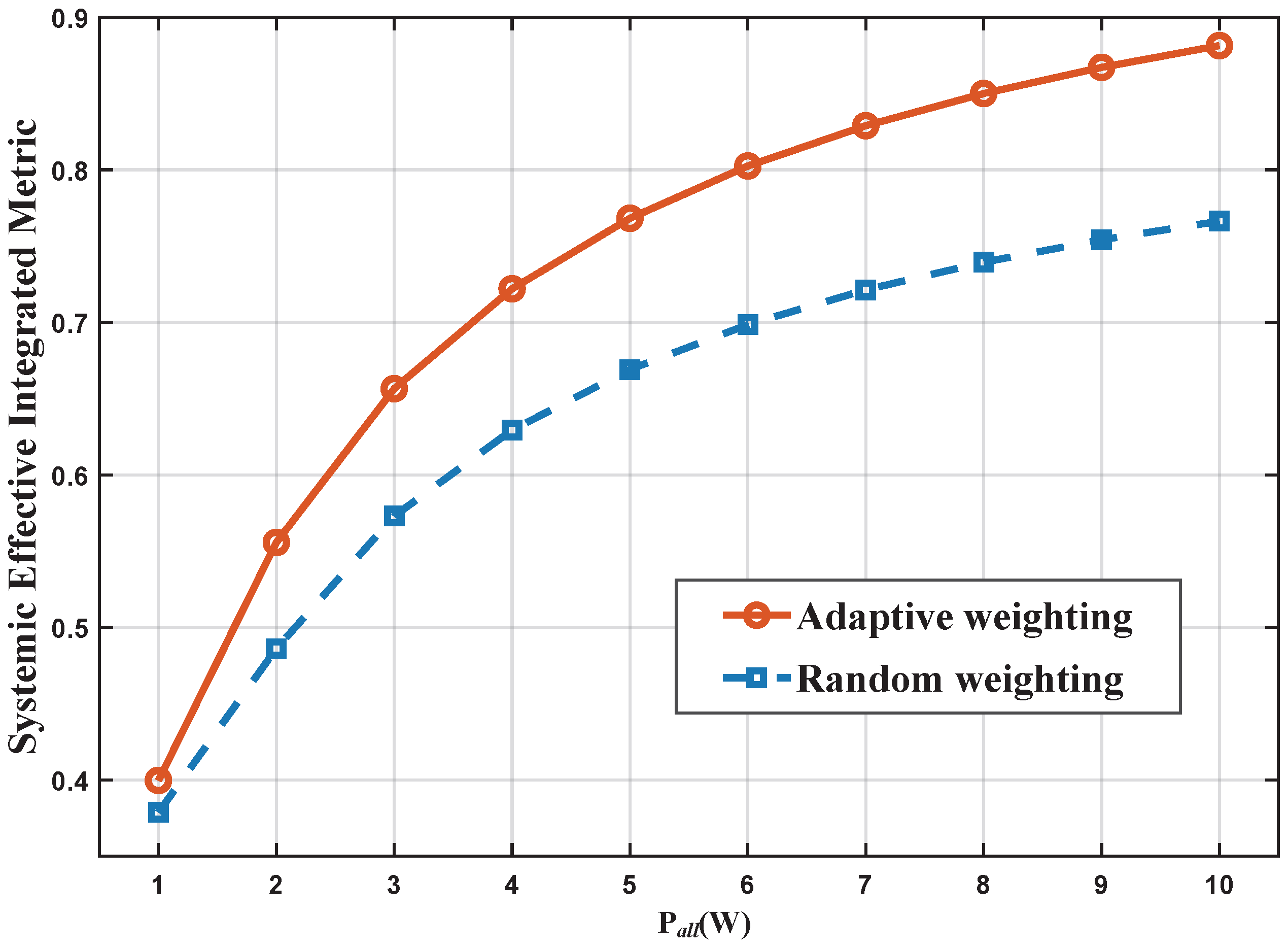
Figure 6 compares entropy-regularized adaptive weighting with random weight selection over P all [ 1 , 10 ] W. Both curves increased rapidly in the low-power region and flattened as the power grew. Adaptive weighting improved the SEIM from approximately 0.40 to 0.88, while random weighting increased it from approximately 0.38 to 0.77. The gap expanded from about 0.02 at 1 W to more than 0.10 at 10 W. The entropy-regularized update repeatedly aligned the weight vector with the normalized covariance performance, whereas random selection frequently assigned excessive weight to a component that offered limited marginal improvement at the current operating point.
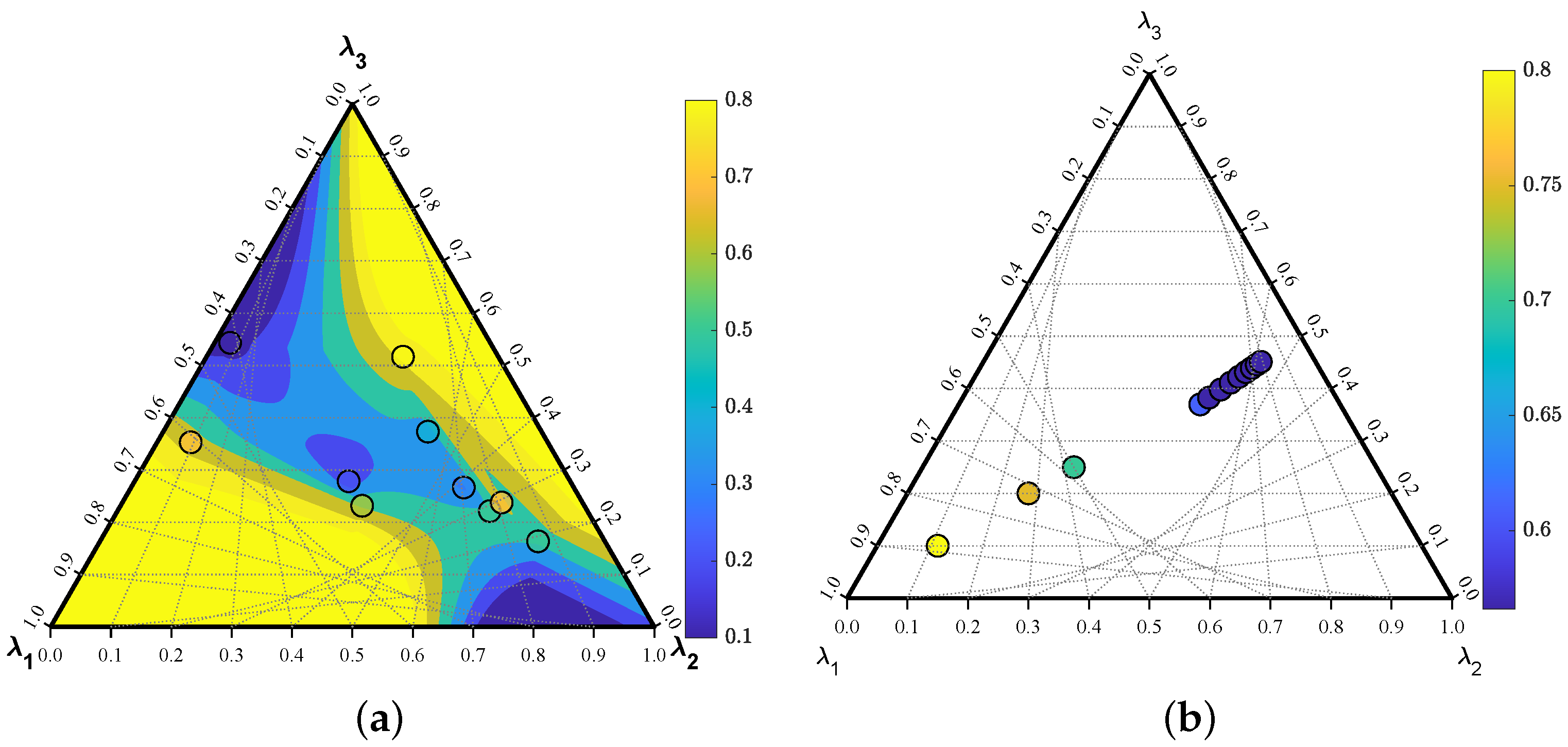
Figure 7 represents the objective-weight simplex defined by λ 1 + λ 2 + λ 3 = 1 , where ( λ 1 , λ 2 , λ 3 ) = ( λ c , λ τ , λ f D ) . Each vertex assigned all scalarization weight to one normalized component. Interior points assigned nonzero weights to all three components.
Figure 7a overlays the evaluated weight points on the SEIM surface. The colored contours show that the integrated metric was sensitive to both the communication-to-sensing split and the division between the delay and Doppler weights. High-SEIM regions extend along the interior and two edges of the simplex, while lower values appear where one component received a weight that was poorly matched to the current covariance response. The evaluated circles cover communication-oriented, delay-oriented, Doppler-oriented, and mixed scalarizations.
Figure 7b shows the weight vectors produced by the adaptive iterations. The early points span a broad portion of the simplex and exhibit SEIM values from approximately 0.56 to 0.80. Subsequent points formed a compact interior cluster with nonzero communication, delay, and Doppler weights. The cluster followed from the entropy term in Equation (46), which discourages vertex solutions, and from the damping factor in Equation (49), which limits the distance between consecutive weight vectors. The figure represents the trajectory of the centralized adaptive scalarization in objective-weight space.

4.6. Comparative Analysis of Holistic Optimization Methods

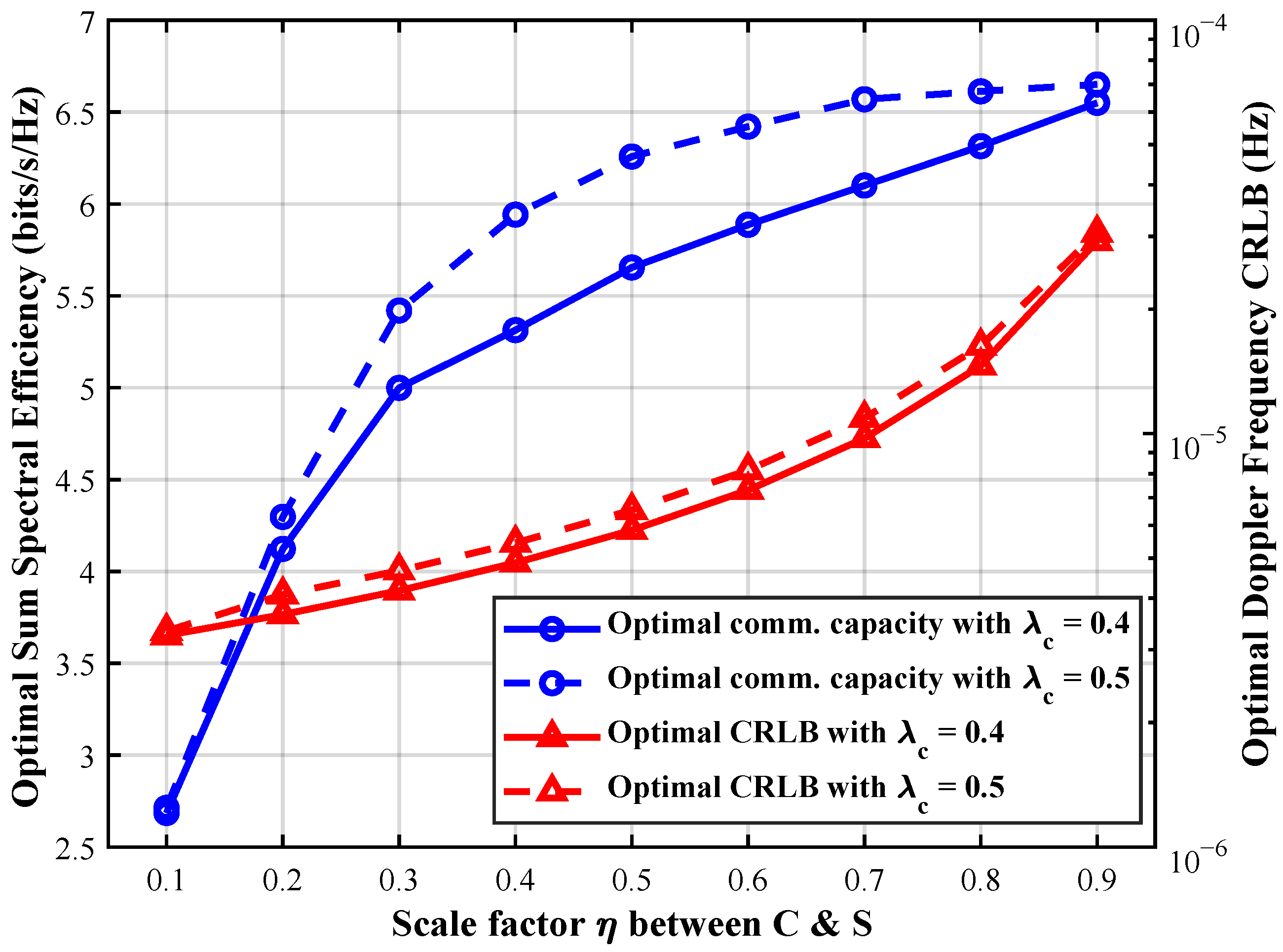
The final experiments evaluated power partitioning, communication-normalized sensing degradation, and beamforming benchmarks under common system configurations. The power-partition factor η [ 0 , 1 ] is defined by P c = η P all and P r = ( 1 η ) P all . Figure 8 plots the communication sum spectral efficiency on the left axis and Doppler CRLB on the logarithmic right axis. For both λ c = 0.4 and λ c = 0.5 , increasing η from 0.1 to 0.9 raised the communication value from approximately 2.7 to more than 6.5 bit/s/Hz. The initial rise was steep because additional communication power directly improved the user SINRs. The slope decreased beyond η = 0.5 as multi-user interference became more influential.
The Doppler CRLB increased with η because the dedicated radar power decreased. Its growth remained gradual over the middle of the interval since the communication covariances also illuminated the target through the second term of J f D in Equation (20). Near η = 0.9 , the radar allocation became small, and the CRLB rose more rapidly. The λ c = 0.5 setting yielded a higher communication curve together with a slightly higher Doppler CRLB, which is consistent with its stronger communication priority.
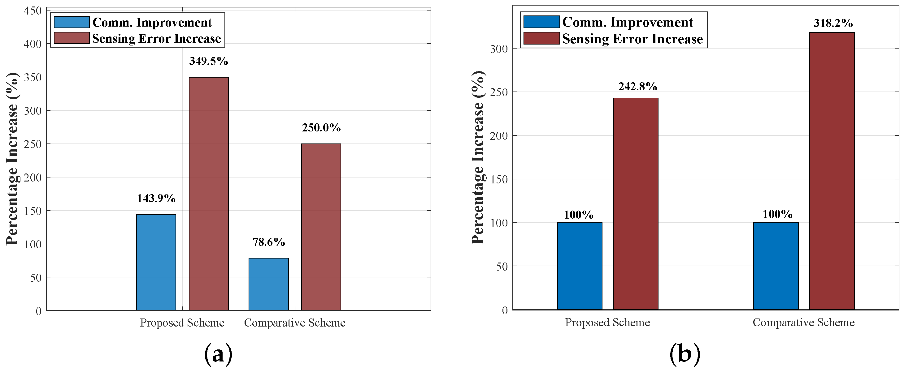
Let Δ C denote the percentage communication improvement relative to the common reference design, and let Δ S denote the corresponding percentage increase in the sensing error. Figure 9a reports the raw changes. The proposed scheme provided a 143.9 % communication improvement and a 349.5 % sensing error increase. The comparative scheme provided a 78.6 % communication improvement and a 250.0 % sensing error increase. The proposed design therefore moved farther along both axes of the C-S tradeoff.
Figure 9b compares the sensing cost after equalizing the communication improvement. The normalization is Δ S eq = 100 Δ S / Δ C . At a common 100 % communication improvement, the proposed and comparative schemes produced sensing error increases of 242.8 % and 318.2 % , respectively. The reduction of 75.4 percentage points means that the proposed covariance and weight updates required less sensing degradation for the same communication improvement at this operating point.
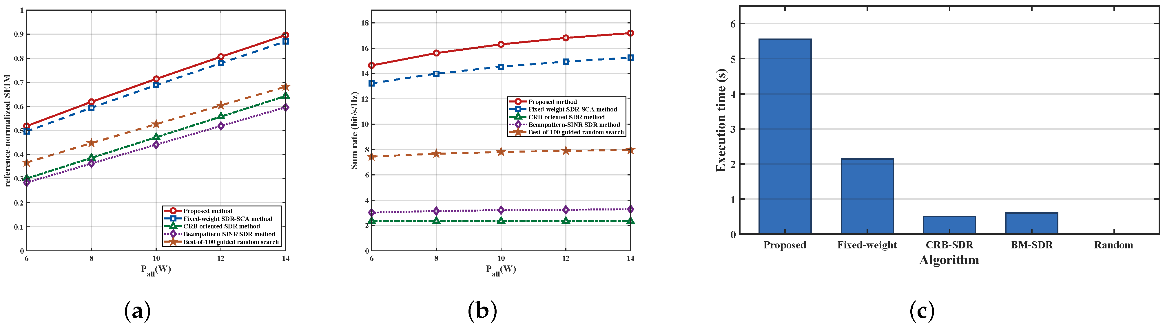
Figure 10 compares five representative beamforming strategies. The proposed method denotes the adaptive alternating SDR-SCA scheme with entropy-regularized objective-weight updates. The fixed-weight SDR–SCA method (fixed weight) uses the same covariance optimization framework but keeps the objective weights unchanged. The CRB-oriented SDR method (CRB-SDR) prioritizes delay–Doppler estimation accuracy, whereas the beampattern–SINR SDR method (BM-SDR) designs the transmit covariance according to the sensing beampattern while satisfying the communication SINR constraints. The best-of-100 guided random search (random) generates multiple channel- and target-guided feasible candidates and selects the one with the highest integrated performance.
Figure 10a compares the reference-normalized SEIM versus the total transmit power. For cross-power comparison, all operating points were normalized using the common reference boundaries obtained at P all = 14 W and the same evaluation weights. The proposed method achieved the highest SEIM over the entire power range, increasing from approximately 0.52 at 6 W to 0.90 at 14 W, followed closely by fixed weight. Random provided intermediate performance, while CRB-SDR and BM-SDR remained lower because their objectives emphasized sensing accuracy or beampattern matching rather than the complete rate–delay–Doppler tradeoff. The curves continued to increase at 14 W because the sensing-information terms still benefited from additional transmit power, partly offsetting the diminishing growth of the communication component.
Figure 10b further compares the achievable sum spectral efficiency of the same methods. The proposed method increased from approximately 14.6 to 17.2 bit/s/Hz as P all grew from 6 to 14 W, while fixed weight followed the same trend at a lower level. Random achieved a moderate sum spectral efficiency of about 7.4 8.0 bit/s/Hz. In contrast, BM-SDR and CRB-SDR remained at relatively low communication rates because their additional power was mainly directed toward sensing-oriented objectives rather than communication rate maximization. The gradually reduced slope of the proposed and fixed-weight curves reflects the diminishing rate gain caused by the logarithmic rate function and residual multi-user interference at higher transmit power.
Figure 10c compares the measured execution times of the five methods at P all = 10 W over eight paired channel realizations. The reported times include method initialization, model construction, convex optimization, rank recovery, feasibility checking, and final candidate evaluation. The proposed method required the highest average execution time of approximately 5.55 s, followed by fixed weight at about 2.14 s, because adaptive objective-weight updates require additional joint SDR-SCA iterations before convergence. CRB-SDR and BM-SDR required only about 0.51 s and 0.61 s, respectively, owing to their simpler sensing-oriented convex formulations, while random incurred negligible computational cost because it avoids iterative covariance optimization. These results show that the performance gain of the proposed adaptive design was obtained at the expense of higher computational complexity, yielding a clear performance–complexity tradeoff among the compared methods.

5. Conclusions

This paper developed an adaptive multi-objective beamforming framework for a MIMO-ISAC downlink that jointly serves terrestrial users and senses a low-altitude UAV target. The proposed formulation jointly accounts for multi-user sum spectral efficiency and delay–Doppler sensing accuracy through conditional CRLBs that incorporate waveform energy, effective bandwidth, coherent duration, target-direction gain, and two-way radar propagation. By evaluating the communication, delay information, and Doppler information boundaries over a common feasible set, the three performance measures are normalized and combined into a dimensionless SEIM. The resulting covariance-domain problem is addressed through SDR and alternating SCA, while an entropy-regularized softmax update with damping adaptively adjusts the objective weights during the iterative optimization. Numerical results demonstrated the effects of the transmit power, receive array size, user loading, SINR requirements, power partition, and objective weighting and showed that the proposed scheme provided a favorable C&S tradeoff compared with the considered benchmark methods.
Several limitations of the present formulation also indicate directions for further investigation. First, perfect CSI was assumed at the base station, whereas practical low-altitude links are subject to channel estimation errors and mobility-induced CSI aging; robust designs under imperfect CSI therefore constitute an important extension. Second, the current model adopts far-field planar-wave steering, which is appropriate for the moderate-aperture operating regime considered here but does not capture spherical-wave propagation in near-field or XL-MIMO deployments, as discussed in [28]; extending the framework to near-field ISAC is a relevant future direction. Third, the sensing model considers a single tracked target, while practical low-altitude networks may involve multiple UAVs or other simultaneously illuminated objects; multi-target sensing would require joint treatment of target separation, mutual interference, and additional spatial DoF allocation. In addition, practical NR/IMT-2030-oriented deployment would impose further physical-layer constraints on the feasible waveform and resource configuration, including the carrier frequency, channel bandwidth and numerology, transmit power and spectral emission limits, TDD frame structure, reference signal overhead, and RF hardware limitations. Finally, the C&S power partition was prescribed through the parameter η and analyzed parametrically rather than jointly optimized with the beamformers. Future work will therefore investigate the joint adaptation of beamforming, C&S power partition, and potentially the transmission duty cycle under dynamic channel, sensing, and implementation constraints.

Author Contributions

Conceptualization, B.Y. and Y.H.; methodology, B.Y.; software, B.Y.; validation, B.Y., Y.H. and X.F.; formal analysis, B.Y.; investigation, B.Y.; resources, Y.H., X.F. and C.W.; data curation, B.Y.; writing—original draft preparation, B.Y.; writing—review and editing, B.Y., Y.H., X.F. and C.W.; visualization, B.Y.; supervision, Y.H., X.F. and C.W.; project administration, Y.H.; funding acquisition, Y.H. All authors have read and agreed to the published version of the manuscript.

Funding

This research was funded by the National Natural Science Foundation of China (grant numbers 62502036, U24B20117, 62172027, U2368202, and 62102019).

Data Availability Statement

The original contributions presented in this study are included in the article. Further inquiries can be directed to the corresponding author.

Conflicts of Interest

Author Chang Wang was employed by State Grid Jibei Electric Power Company Limited. The remaining authors declare that the research was conducted in the absence of any commercial or financial relationships that could be construed as a potential conflict of interest.

Appendix A. Proof of Theorem 1

Consider one scalar waveform component u q ( t ) centered at its energy centroid t ¯ q . Apart from constants that are common to the two derivatives, its noise-free received signal is
μ q ( t ) = α q u q ( t τ ) e j 2 π f D ( t t ¯ q ) .
At the true parameter values, we have
μ q ( t ) τ = α q u ˙ q ( t ) e j 2 π f D ( t t ¯ q ) .
Similarly, we also have
μ q ( t ) f D = j 2 π ( t t ¯ q ) α q u q ( t ) e j 2 π f D ( t t ¯ q ) .
Substitution into Equation (15) shows that the cross-information contributed by this component is proportional to the centered time–frequency moment
Ξ q = j 2 π ( t t ¯ q ) u ˙ q * ( t ) u q ( t ) d t .
Thus, centering the energy alone is not sufficient to make the delay–Doppler cross-term vanish.
For the radar waveform, differentiating s n , χ ( t ) shows that Ξ r , χ is odd in the chirp-slope sign χ . The two members of the CPI have equal energy and identical support. Their combined moment satisfies
Ξ r , + 1 + Ξ r , 1 = 0 .
For the communication waveform, the symbols are independent and zero-mean, the symbol times are centered about zero, and the pulse-shaping filter has an even energy envelope. The diagonal symbol terms therefore occur in symmetric time pairs, whereas all cross-symbol terms have zero expectation. Consequently, we have
E { Ξ c , k } = 0 , k = 1 , , K .
The orthogonality assumptions in Section 2 remove cross-component contributions. Summing Equations (A5) and (A6) therefore gives E { J τ f D } = 0 , which proves the stated conditional result. If these pairing and symmetry conditions are not satisfied, then J τ f D must be included, and the full FIM must be inverted.

References

  1. Fang, X.; Feng, W.; Chen, Y.; Ge, N.; Zhang, Y. Joint Communication and Sensing Toward 6G: Models and Potential of Using MIMO. IEEE Internet Things J. 2023, 10, 4093–4116. [Google Scholar] [CrossRef] [Scilit]
  2. Liu, R.; Li, M.; Luo, H.; Liu, Q.; Swindlehurst, A.L. Integrated Sensing and Communication with Reconfigurable Intelligent Surfaces: Opportunities, Applications, and Future Directions. IEEE Wirel. Commun. 2023, 30, 50–57. [Google Scholar] [CrossRef] [Scilit]
  3. Zhu, X.; Liu, J.; Lu, L.; Zhang, T.; Qiu, T.; Wang, C.; Liu, Y. Enabling Intelligent Connectivity: A Survey of Secure ISAC in 6G Networks. IEEE Commun. Surv. Tutor. 2025, 27, 748–781. [Google Scholar] [CrossRef] [Scilit]
  4. Su, X.; Song, J.; Liu, Z.; Guan, X.; Yang, F.; Dong, Y.; Zhang, H.; Wang, J.; Pan, C.; Zhang, X. Optical Integrated Sensing and Communication: From Theory to Practice. Tsinghua Sci. Technol. 2025. [Google Scholar] [CrossRef] [Scilit]
  5. Pucci, L.; Paolini, E.; Giorgetti, A. System-Level Analysis of Joint Sensing and Communication Based on 5G New Radio. IEEE J. Sel. Areas Commun. 2022, 40, 2043–2055. [Google Scholar] [CrossRef] [Scilit]
  6. Hua, H.; Han, T.X.; Xu, J. MIMO Integrated Sensing and Communication: CRB-Rate Tradeoff. IEEE Trans. Wirel. Commun. 2024, 23, 2839–2854. [Google Scholar] [CrossRef] [Scilit]
  7. Liu, F.; Yuan, W.; Masouros, C.; Yuan, J. Radar-Assisted Predictive Beamforming for Vehicular Links: Communication Served by Sensing. IEEE Trans. Wirel. Commun. 2020, 19, 7704–7719. [Google Scholar] [CrossRef] [Scilit]
  8. Cui, Y.; Ding, H.; Ma, Y.; Li, X.; Zhang, H.; Fang, Y. Energy-Efficient Integrated Sensing and Communication in Collaborative Millimeter Wave Networks. IEEE Trans. Wirel. Commun. 2025, 24, 2341–2357. [Google Scholar] [CrossRef] [Scilit]
  9. Yin, L.; Liu, Z.; Shankar, M.R.B.; Alaee-Kerahroodi, M.; Clerckx, B. Integrated Sensing and Communications Enabled Low Earth Orbit Satellite Systems. IEEE Netw. 2024, 38, 252–258. [Google Scholar] [CrossRef] [Scilit]
  10. Gu, M.X.; Lee, M.C.; Liu, Y.S.; Lee, T.S. Design and Analysis of Frequency Hopping-Aided FMCW-Based Integrated Radar and Communication Systems. IEEE Trans. Commun. 2022, 70, 8416–8432. [Google Scholar] [CrossRef] [Scilit]
  11. Liyanaarachchi, S.D.; Riihonen, T.; Barneto, C.B.; Valkama, M. Optimized Waveforms for 5G–6G Communication With Sensing: Theory, Simulations and Experiments. IEEE Trans. Wirel. Commun. 2021, 20, 8301–8315. [Google Scholar] [CrossRef] [Scilit]
  12. Dong, F.; Wang, W.; Hu, Z.; Hui, T. Low-Complexity Beamformer Design for Joint Radar and Communications Systems. IEEE Commun. Lett. 2021, 25, 259–263. [Google Scholar] [CrossRef] [Scilit]
  13. Liu, F.; Liu, Y.F.; Li, A.; Masouros, C.; Eldar, Y.C. Cramér–Rao Bound Optimization for Joint Radar–Communication Beamforming. IEEE Trans. Signal Process. 2022, 70, 240–253. [Google Scholar] [CrossRef] [Scilit]
  14. Liu, Y.; Liao, G.; Yang, Z.; Xu, J. Multiobjective Optimal Waveform Design for OFDM Integrated Radar and Communication Systems. Signal Process. 2017, 141, 331–342. [Google Scholar] [CrossRef] [Scilit]
  15. Nguyen, N.T.; Shlezinger, N.; Eldar, Y.C.; Juntti, M. Multiuser MIMO Wideband Joint Communications and Sensing System With Subcarrier Allocation. IEEE Trans. Signal Process. 2023, 71, 2997–3013. [Google Scholar] [CrossRef] [Scilit]
  16. Barneto, C.B.; Liyanaarachchi, S.D.; Heino, M.; Riihonen, T.; Valkama, M. Full Duplex Radio/Radar Technology: The Enabler for Advanced Joint Communication and Sensing. IEEE Wirel. Commun. 2021, 28, 82–88. [Google Scholar] [CrossRef] [Scilit]
  17. Xu, C.; Zhang, S. MIMO Integrated Sensing and Communication Exploiting Prior Information. IEEE J. Sel. Areas Commun. 2024, 42, 2306–2321. [Google Scholar] [CrossRef] [Scilit]
  18. Zhu, Q.; Li, M.; Liu, R.; Liu, Q. Joint Transceiver Beamforming and Reflecting Design for Active RIS-Aided ISAC Systems. IEEE Trans. Veh. Technol. 2023, 72, 9636–9640. [Google Scholar] [CrossRef] [Scilit]
  19. Su, N.; Liu, F.; Masouros, C. Sensing-Assisted Eavesdropper Estimation: An ISAC Breakthrough in Physical Layer Security. IEEE Trans. Wirel. Commun. 2024, 23, 3162–3174. [Google Scholar] [CrossRef] [Scilit]
  20. He, X.; Huang, L. Joint MIMO Communication and MIMO Radar Under Different Practical Waveform Constraints. IEEE Trans. Veh. Technol. 2020, 69, 16342–16347. [Google Scholar] [CrossRef] [Scilit]
  21. Xiao, Z.; Zeng, Y. Waveform Design and Performance Analysis for Full-Duplex Integrated Sensing and Communication. IEEE J. Sel. Areas Commun. 2022, 40, 1823–1837. [Google Scholar] [CrossRef] [Scilit]
  22. Liu, W.; Hou, X.; Liu, J.; Chen, L. Low-Overhead Sensing RS Design for Integrated Sensing and Communication (ISAC). In Proceedings of the 2025 IEEE Wireless Communications and Networking Conference (WCNC), Milan, Italy, 24–27 March 2025; pp. 1–6. [Google Scholar] [CrossRef] [Scilit]
  23. Zhang, L.; Lei, X.; Ma, T.; Niu, H.; Yuen, C. Joint User Localization, Channel Estimation, and Pilot Optimization for RIS-ISAC. IEEE Trans. Wirel. Commun. 2024, 23, 19302–19316. [Google Scholar] [CrossRef] [Scilit]
  24. Rao, C.R. Information and the Accuracy Attainable in the Estimation of Statistical Parameters. Bull. Calcutta Math. Soc. 1945, 37, 81–91. [Google Scholar]
  25. Kay, S.M. Fundamentals of Statistical Signal Processing, Volume I: Estimation Theory; Prentice Hall PTR: Upper Saddle River, NJ, USA, 1993. [Google Scholar]
  26. Mao, W.; Lu, Y.; Chi, C.Y.; Ai, B.; Zhong, Z.; Ding, Z. Communication-Sensing Region for Cell-Free Massive MIMO ISAC Systems. IEEE Trans. Wirel. Commun. 2024, 23, 12396–12411. [Google Scholar] [CrossRef] [Scilit]
  27. Grant, M.; Boyd, S. CVX: Matlab Software for Disciplined Convex Programming, Version 2.2; CVX Research, Inc.: Austin, TX, USA, 2020; Available online: https://cvxr.com/cvx (accessed on 10 August 2026).
  28. Wang, H.; Yan, T.; Zhou, N.; Li, X.; Wen, F.; Du, W. Enhanced Polar-Domain Channel Estimation for Near-Field XL-MIMO in Low-SNR Scenarios. IEEE Trans. Veh. Technol. 2025, 74, 19407–19419. [Google Scholar] [CrossRef] [Scilit]
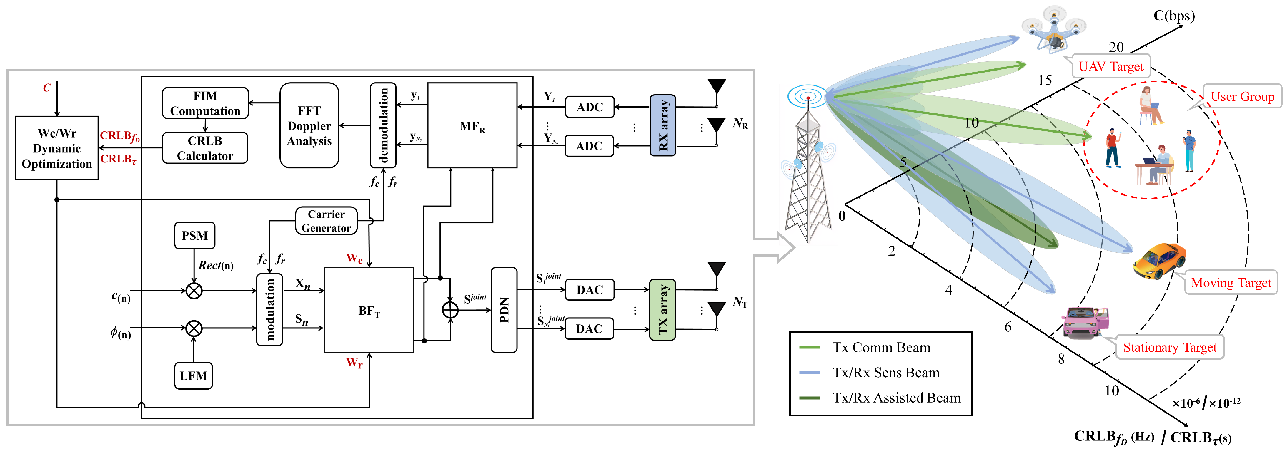
Figure 1. System architecture and signal processing of the multiple-input multiple-output integrated sensing and communication (MIMO-ISAC) framework. ⨂ and ⨁ denote signal multiplication and addition, respectively, while ⋯ denotes omitted intermediate antenna elements.
Electronics 15 04121 g001
Figure 2. Communication- and sensing-oriented transmit beampatterns. (a) Beamforming patterns under communication-oriented design. (b) Beamforming patterns under sensing-oriented design.
Electronics 15 04121 g002
Figure 3. Effects of transmit power, receive array size, user loading, and objective weights on the system effectiveness integrated metric (SEIM). (a) SEIM versus P all for different N r values. (b) SEIM versus N r for different P all values. (c) SEIM versus P all for different K values. (d) SEIM versus P all for different objective weights.
Electronics 15 04121 g003
Figure 4. SEIM versus λ c for different user SINR thresholds γ th .
Electronics 15 04121 g004
Figure 5. SEIM dependence on user loading and communication weight. (a) Metric analysis with various λ c values under different K values. (b) Metric analysis with various K values under different λ c values.
Electronics 15 04121 g005
Figure 6. SEIM under adaptive and random objective-weight selection.
Electronics 15 04121 g006
Figure 7. Objective-weight adaptation on the three-component simplex. (a) SEIM surface and evaluated objective weights. (b) Objective weights returned by the adaptive iterations.
Electronics 15 04121 g007
Figure 8. Performance balance between communication and sensing.
Electronics 15 04121 g008
Figure 9. Communication improvement and sensing error increase before and after equal communication normalization. (a) Comparison of the proposed scheme with the reference scheme. (b) Comparison of the schemes after incremental normalization.
Electronics 15 04121 g009
Figure 10. Performance and computational complexity comparison of representative beamforming methods. (a) Reference-normalized SEIM versus total transmit power. (b) Sum spectral efficiency versus total transmit power. (c) Average execution time of the compared methods.
Electronics 15 04121 g010
Table 1. Comparative summary of representative integrated sensing and communication (ISAC) optimization methods.
ReferenceObjectiveApproachMain Distinction
[12]Beampattern-SINR designIterative convex relaxationBeampattern-based sensing without parameter estimation CRLB optimization
[13]Estimation accuracy optimizationCRLB-oriented beamformingSensing-oriented objective with communication QoS constraints
[14]CRB-capacity tradeoffWeighted multi-objective optimizationPrescribed objective weights
[15]C&S resource allocationSubcarrier allocationFrequency-domain resource partitioning
[17]Prior-aided sensing accuracyPosterior CRLB optimizationRelies on prior target information
[18]RIS-aided NLoS sensingJoint transceiver and RIS designRequires RIS configuration and associated CSI
[19]Physical-layer securityDOA-assisted secure beamformingSecurity-oriented design based on sensing-derived DOA
This workRate-delay-Doppler tradeoffAdaptive SDR-SCA optimizationBoundary-normalized SEIM with adaptive objective-weight selection
Table 2. Simulation parameters.
SymbolDescriptionValue
N t Transmit antennas8
N r Receive antennas8
KCommunication users4
d f 0 / c 0 Normalized antenna spacing 0.5
K c , k Rician factor5 ( 6.99 dB)
σ c , k 2 User noise power 1.26 × 10 10 W
P all Nominal total power10 W
Total power sweep6–14 W
η Comm. power fraction0.5
γ th Minimum user SINR0.5 ( 3.01 dB)
d 0 Nominal user distances [ 80 , 95 , 115 , 130 ] m
ϑ 0 Nominal user azimuths [ 50 , 15 , 20 , 55 ]
ϵ d , k Relative distance perturbation N ( 0 , 0.025 2 )
δ ϑ , k Azimuth perturbation N ( 0 , ( 2 ) 2 )
G t , G r Antenna gains10 dBi
σ ¯ Target RCS 1 m 2
r tar BS–UAV slant range100 m
θ Predicted target azimuth 30
ψ Reflection phase U ( 0 , 2 π )
N GR Gaussian randomization trials100
Disclaimer/Publisher’s Note: The statements, opinions and data contained in all publications are solely those of the individual author(s) and contributor(s) and not of MDPI and/or the editor(s). MDPI and/or the editor(s) disclaim responsibility for any injury to people or property resulting from any ideas, methods, instructions or products referred to in the content.