Integrated Vibration Suppression for Industrial Manipulators via Disturbance Observer and Partial Eigenstructure Assignment

Abstract

Residual vibration of industrial manipulators can limit positioning efficiency and dynamic accuracy during high-speed motion. This study develops an integrated vibration-suppression framework for a rigid-link manipulator with flexible-joint dynamics. A controller-oriented rigid–flexible model with lumped disturbances is established, and a disturbance observer (DOB) is employed as the inner-loop compensation layer under a small-gain robustness constraint. On the compensated nominal model, partial eigenstructure assignment (PESA) selectively increases the damping of the retained flexible modes while preserving the rigid-body eigenstructure associated with trajectory tracking. A pose-dependent gain-scheduling mechanism further updates the PESA feedback gain to accommodate configuration-dependent modal-frequency variation. Numerical comparisons with conventional PID, standalone DOB, and standalone PESA demonstrate improved residual-vibration attenuation and settling behavior. Hardware tests on an Aubo i5 manipulator, with 16-channel responses directly acquired under the respective control configurations, further show an approximately 80% reduction in the representative low-frequency vibration amplitude relative to the PID baseline under the considered operating condition.

1. Introduction

Six-degree-of-freedom industrial manipulators are widely used in advanced manufacturing fields, where positioning speed and dynamic accuracy directly affect production efficiency. To achieve lightweight design and higher load-to-weight ratios, modern manipulators increasingly adopt lightweight links and compliant joint/transmission components [1]. However, high-acceleration trajectories and frequent start–stop operations can excite residual vibration due to structural flexibility, nonlinear disturbances, and resonance coupling, which limits dynamic accuracy and motion stability.

To analyze and suppress vibration in flexible manipulators, existing studies have investigated structural modeling and vibration-control approaches. FEA and modal identification techniques are widely used to characterize flexible dynamics and provide information for controller design [2,3,4,5,6]. Input-shaping methods reduce residual vibration through reference modification but depend on accurate modal information and may degrade under varying operating conditions [7,8]. Active vibration control methods provide direct vibration suppression through additional sensing or actuation, but may increase implementation complexity and cost [9,10].

To address vibration caused by flexible dynamics, input-shaping methods have been widely used for residual-vibration suppression due to their low computational cost and compatibility with closed-loop systems [7]. However, fixed-frequency shapers are sensitive to modal variation, and adaptive shaping methods may suffer from online frequency estimation delays under rapidly changing operating conditions [8,9,10]. Active control approaches, including pole placement and optimal control methods, can improve vibration damping, but their effectiveness depends on accurate state information and may be affected by sensing noise and implementation complexity [11,12,13]. Intelligent control methods have also been investigated for vibration suppression [14,15], but their computational requirements and stability guarantees remain challenging for millisecond-level industrial control applications. Therefore, existing approaches still face limitations in simultaneously handling modal variation, disturbance rejection, and practical implementation constraints in industrial manipulators.

Recent vibration-suppression studies for complex flexible and coupled mechanical systems have also explored control mechanisms beyond conventional trajectory-oriented feedback. Vindigni et al. [16] investigated piezoelectric-stack-based passive and active vibration suppression for flexible satellite solar panels and compared shunt-circuit damping with active filtered-PID control, illustrating the trade-off between vibration attenuation performance and actuation requirements. Zhao et al. [17] studied a nonlinear coupled beam system subjected to multiple excitation sources and showed, through theoretical and experimental analysis, that appropriately designed nonlinear coupling can modify vibration transfer and suppress structural responses under multi-source excitation. These studies highlight the importance of considering structural flexibility, coupling mechanisms, excitation characteristics, and implementation constraints when selecting a vibration-suppression strategy for complex mechanical systems. For industrial manipulators, these issues are further complicated by configuration-dependent modal variation and multi-source disturbances, which motivates the disturbance-compensation and modal-control framework considered in this work.

To improve robustness against modeling errors and external disturbances, disturbance observer (DOB)-based methods have been widely applied in manipulator control due to their disturbance estimation and compensation capability [16,18]. However, DOB performance is constrained by the trade-off between disturbance-rejection bandwidth and robustness against measurement noise and unmodeled high-frequency dynamics [19,20]. Therefore, DOB alone cannot provide selective damping of structural resonance modes, leaving frequency-dependent vibration suppression as a remaining challenge [21].

Recent studies on active vibration control and eigenstructure assignment have shown that partial eigenstructure assignment (PESA) can modify selected modal characteristics through closed-loop eigenstructure design [22]. However, most existing PESA-based controllers assume relatively fixed modal parameters. For industrial manipulators, rigid–flexible coupling, configuration-dependent modal variation, and robustness limitations of the disturbance-rejection layer make it difficult to simultaneously achieve disturbance compensation and adaptive flexible-mode suppression.

Existing vibration-control approaches address different aspects of rigid–flexible manipulator control but have individual limitations. Input-shaping methods provide low-cost vibration attenuation but are sensitive to modal-frequency variation caused by configuration changes [23]. DOB-based methods compensate for equivalent disturbances and model mismatch within the observer bandwidth but cannot directly increase structural modal damping. Pole-placement and eigenstructure-assignment methods can reshape flexible-mode dynamics, but fixed-gain designs may degrade under posture-dependent modal variation. Gain scheduling improves adaptation to configuration changes but does not independently compensate for nonlinear disturbances and model uncertainties.

Based on these limitations, the proposed DOB–PESA framework coordinates three control functions: the DOB provides disturbance compensation and plant nominalization, the PESA layer increases damping of selected flexible modes, and the pose-dependent gain scheduling updates modal feedback gains according to configuration variation. Therefore, the proposed architecture simultaneously addresses disturbance-induced oscillation, residual flexible-mode vibration, and modal-frequency drift.

Eigenstructure-assignment methods are suitable for selective modal damping by modifying closed-loop poles and eigenvectors [22]. However, conventional fixed-gain PESA designs rely on nominal modal characteristics and may lose effectiveness when flexible-mode frequencies vary with manipulator configuration [24]. This motivates the introduction of pose-dependent gain scheduling in the proposed framework.

The methodological contribution of this work lies in establishing explicit design dependencies among DOB, PESA, and gain scheduling [24]. The DOB provides a compensated nominal basis for PESA synthesis under bounded uncertainty; PESA then performs selective modal damping on the dominant flexible modes; and the gain-scheduling mechanism updates the modal feedback gain according to configuration-dependent frequency variation [24]. This sequential coupling enables coordinated disturbance rejection, modal damping, and posture adaptation.

Accordingly, the unresolved control problem is how to coordinate robustness-constrained disturbance compensation, selective damping of dominant flexible modes, and adaptation to posture-dependent modal drift without unnecessarily modifying the rigid-body motion characteristics. The specific contributions of this work are summarized as follows:

(1) A DOB-based nominalization layer is developed for the rigid–flexible manipulator, where model mismatch, nonlinear friction, coupling effects, and external disturbances are represented through a lumped-disturbance channel with Q-filter robustness constraints.

(2) A PESA controller is designed on the DOB-compensated nominal model to selectively damp retained flexible modes while preserving rigid-body tracking dynamics.

(3) A pose-dependent gain-scheduling mechanism updates the PESA feedback gain according to modal-frequency variation, maintaining vibration attenuation under configuration changes.

2. Analysis of Vibration Mechanisms in Industrial Manipulators

This section summarizes the dynamic and modal quantities required for the subsequent controller formulation.

2.1. Dynamic Modeling

The rigid-body dynamics are formulated using a Jacobian-based Lagrangian representation [25]. For the i-th link, the angular and linear velocities are expressed through the corresponding Jacobian mappings as

$$v_i=J_{vi}(q)\dot{q}$$

(1)

$${\omega }_i=J_{\omega i}(q)\dot{q}$$

(2)

where $q$ denotes the joint-configuration vector and $\dot{q}$ is the instantaneous acceleration. J the corresponding link Jacobian. Using the standard Lagrangian formulation [23], the joint-space rigid-body dynamics are written as

$$\tau =M(q)\ddot{q}+C(q,\dot{q})\dot{q}+G(q)+{\tau }_{fric}$$

(3)

Equivalently, the rigid-body dynamics can be written in the standard joint-space form:

$${\tau }_i={\displaystyle {\displaystyle \sum _{j=1}^n}{M}_{ij}}(q){\ddot{q}}_j+{\displaystyle {\displaystyle \sum _{k=1}^n}{\displaystyle \sum _{j=1}^n{c}_{ikj}}}(q){\dot{q}}_k{\dot{q}}_j+G_i(q)+{\tau }_{f,i}+{\tau }_{ext,i}$$

(4)

where ${\displaystyle \sum _{j=1}^n{M}_{ij}}(q){\ddot{q}}_j$, ${\displaystyle \sum _{k=1}^n{\displaystyle \sum _{j=1}^n{c}_{ikj}}}(q){\dot{q}}_k{\dot{q}}_j$, $G_i(q)$, ${\tau }_{f,i}$, and ${\tau }_{ext,i}$ denote the inertia matrix, Coriolis term, gravity torque, friction torque, and external disturbance, respectively.

2.2. Analysis of Multi-Pose Modal Characteristics of the Manipulator

At a given joint configuration q, the natural frequencies and corresponding mode shapes are obtained from the generalized eigenvalue problem:

$$[K(q)-{\omega }_r^2(q)M(q)]{\varphi }_r(q)=0$$

(5)

where $M(q)$ and $K(q)$ are the configuration-dependent mass and stiffness matrices, and ${\varphi }_r(q)$ is the mode shape corresponding to the r-th order mode, which is the eigenvector of the natural frequency ${\omega }_r^2(q)$.

Using the mass-normalized modal matrix, the local dynamics are projected into modal coordinates as

$${\Phi }^{T}M(q)\Phi =I,\hspace{1em}{\Phi }^{T}K(q)\Phi =\mathrm{diag}({\omega }_1^2,\dots ,{\omega }_n^2)$$

(6)

Equations (5) and (6) establish the relationship between the local modal model and the vibration characteristics considered in this study. Equation (5) yields multiple structural eigenpairs and shows that the calculated natural frequencies and mode shapes vary with the configuration-dependent mass and stiffness matrices M(q) and K(q). Equation (6) represents the corresponding modal participation in modal coordinates. The persistence of residual vibration is associated with the lightly damped flexible modes of the flexible-joint system rather than being inferred from the mass–stiffness eigenvalue problem alone. These quantities are subsequently used for retained-mode selection and reduced-order modeling.

2.3. Quantification and Extraction of Vibration-Response Features

In this study, x(t) denotes the acceleration response of an individual measurement channel used for modal-feature extraction. For the hardware validation in Section 4.5, these responses are directly acquired through the 16-channel measurement system, expressed in m/s², and detrended and band-pass filtered before feature extraction [26].

The analytic signal used for instantaneous-frequency estimation is defined by the standard Hilbert-transform relation:

$$z(t)=x(t)+jH[x(t)]=A(t)e^{j\varphi (t)}$$

(7)

where $H[x(t)]$ denotes the Hilbert transform. The corresponding instantaneous frequency is obtained as

$$f_{ins}(t)={\displaystyle \frac{1}{2\pi }}{\displaystyle \frac{d\varphi (t)}{dt}}$$

(8)

During the vibration-decay interval, the modal damping ratio is estimated from the amplitude envelope using

$$\zeta \approx -{\displaystyle \frac{1}{\dot{\varphi }\left(t\right)}}{\displaystyle \frac{d\left(\mathrm{l}\mathrm{n}A\left(t\right)\right)}{dt}}$$

(9)

These extracted quantities support retained-mode characterization and configuration-dependent controller design; they are not treated as a separately validated real-time modal-identification loop in the present study.

3. DOB–PESA-Based Vibration Control

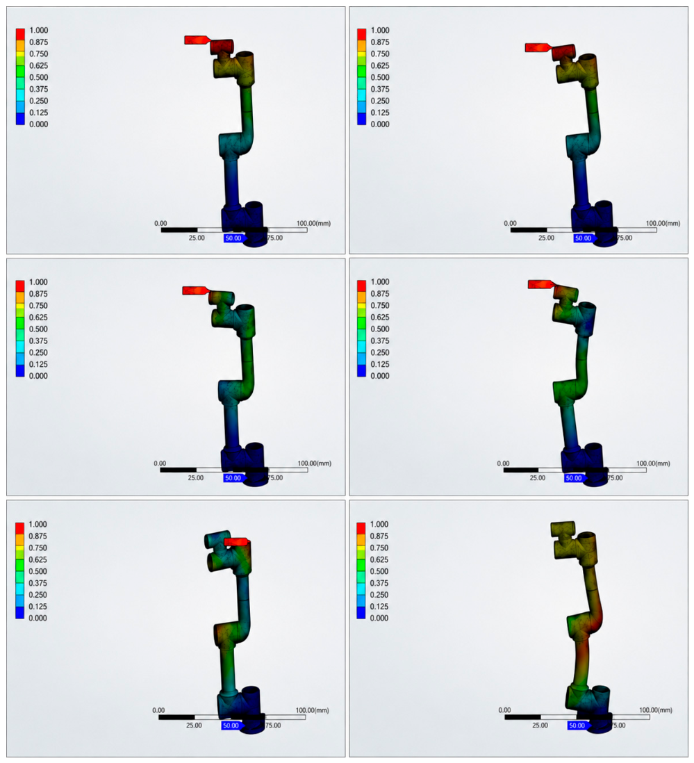
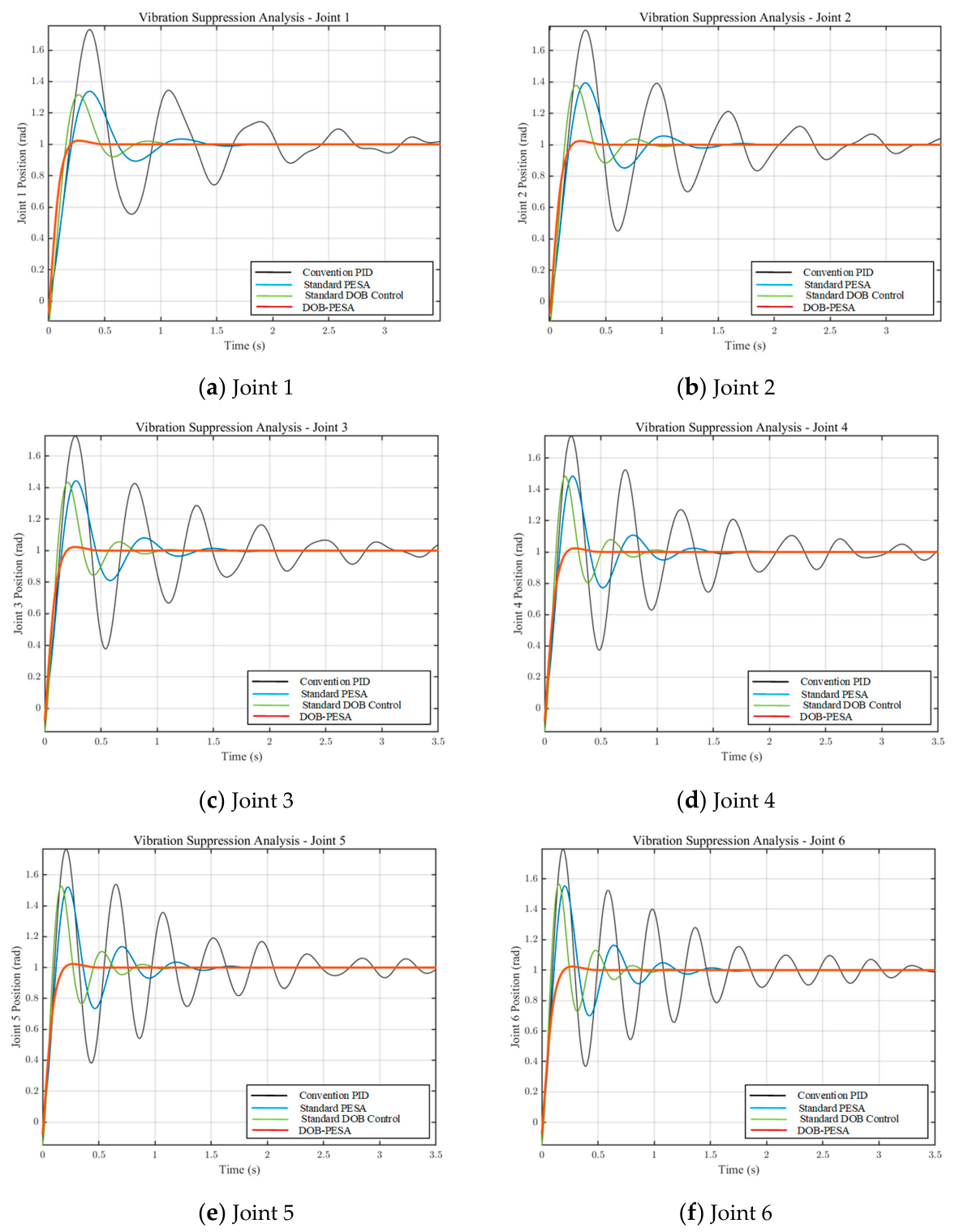
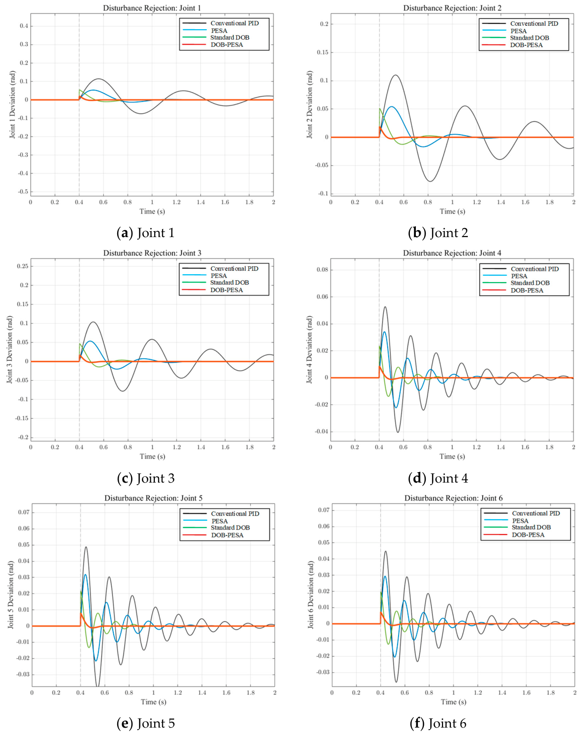
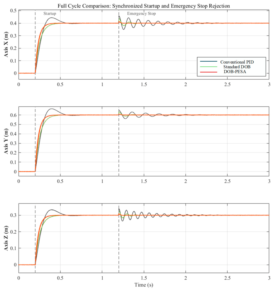
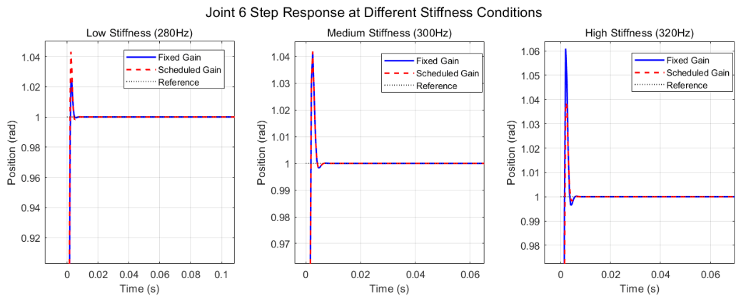
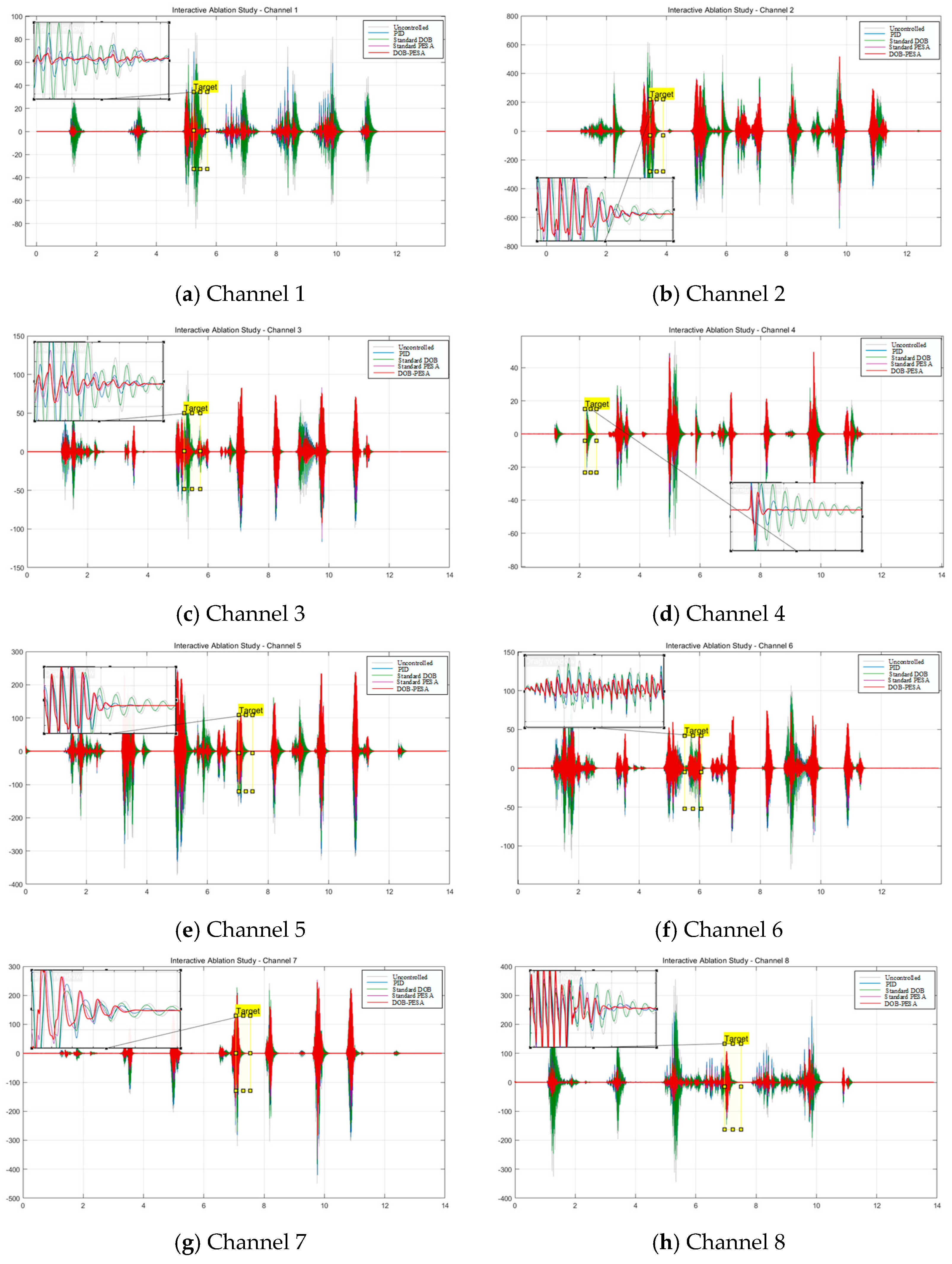
The controller consists of an inner-loop DOB, a PESA modal-feedback layer, and a pose-dependent gain-scheduling mechanism.

3.1. Dynamic Modeling of the Flexible-Joint Manipulator

The manipulator links are modeled as rigid bodies, while the dominant flexibility is represented by the equivalent torsional stiffness and viscous damping of the joint/transmission system. Accordingly, the physical model considered here is a rigid-link manipulator with flexible-joint dynamics rather than a manipulator with structurally flexible links. Using the standard Euler–Lagrange formulation for flexible-joint robots [27,28,29,30,31], the kinetic energy is written as

$$T=T_m+T_l={\displaystyle \frac{1}{2}}{\dot{q}}_m^T{J}_m{\dot{q}}_m+{\displaystyle \frac{1}{2}}{\dot{q}}_l^{T}M\left(q_l\right){\dot{q}}_l$$

(10)

where $q_m$ and $q_l$ denote the motor-side and link-side coordinates, respectively; $J_m$ is the equivalent motor-side inertia matrix; and $M\left(q_l\right)$ is the configuration-dependent link-side inertia matrix.

The potential energy $U$ of the system mainly consists of gravitational potential energy $U_g$ and joint elastic potential energy $U_e$:

$$U=U_g+U_e=G\left(q_l\right)+{\displaystyle \frac{1}{2}}{\left(q_l-N^{-1}{q}_m\right)}^{T}K\left(q_l-N^{-1}{q}_m\right)$$

(11)

With K denoting the equivalent joint stiffness matrix and N the reducer-ratio matrix, the viscous dissipation is

$$D={\displaystyle \frac{1}{2}}{\left({\dot{q}}_l-N^{-1}{\dot{q}}_m\right)}^T{B}_v\left({\dot{q}}_l-N^{-1}{\dot{q}}_m\right)$$

(12)

where Bv is the equivalent viscous damping matrix of the joint. Substituting the above energy function (12) into the generalized Euler–Lagrange Equation yields

$${\displaystyle \frac{d}{dt}}\left({\displaystyle \frac{\partial T}{\partial {\dot{q}}_i}}\right)-{\displaystyle \frac{\partial T}{\partial q_i}}+{\displaystyle \frac{\partial D}{\partial {\dot{q}}_i}}+{\displaystyle \frac{\partial U}{\partial q_i}}={\tau }_i$$

(13)

The corresponding damping contributions for the motor-side and link-side coordinates are

$${\displaystyle \frac{\partial D}{\partial {\dot{q}}_m}}=-N^{-1}{B}_v\left({\dot{q}}_l-N^{-1}{\dot{q}}_m\right)=N^{-1}{B}_v\left(N^{-1}{\dot{q}}_m-{\dot{q}}_l\right)$$

(14)

$${\displaystyle \frac{\partial D}{\partial {\dot{q}}_l}}=B_v\left({\dot{q}}_l-N^{-1}{\dot{q}}_m\right)$$

(15)

Substituting the corresponding elastic and damping terms into Equation (13) yields the coupled motor-side and link-side dynamics:

$$\left\{\begin{array}{l}M(q_l){\ddot{q}}_l+C(q_l,{\dot{q}}_l){\dot{q}}_l+g(q_l)+B_v({\dot{q}}_l-N^{-1}{\dot{q}}_m)+K(q_l-N^{-1}{q}_m)={\tau }_{ext}\hfill \\ J_m{\ddot{q}}_m+N^{-1}{B}_v(N^{-1}{\dot{q}}_m-{\dot{q}}_l)+N^{-1}K(N^{-1}{q}_m-q_l)+F_m({\dot{q}}_m)={\tau }_m\hfill \end{array}\right.$$

(16)

$$g(q_l)={\displaystyle \frac{\partial G(q_l)}{\partial q_l}}$$

(17)

In Equations (16) and (17), $F_m({\dot{q}}_m)$, ${\tau }_{ext}$, and $g(q_l)$ denote the motor-side friction, link-side external disturbance, and gravitational torque, respectively. The motor- and link-side coordinates are coupled through the equivalent stiffness K and damping $B_v$, while N denotes the reducer-ratio matrix and ${\tau }_m$ denotes the motor torque input.

3.2. Establishment of the Linear Nominal Model and the Lumped Disturbance of the System

Within the prescribed workspace and small-deformation range, the flexible-joint dynamics in Equations (16) and (17) are separated into a local nominal component for controller synthesis and an equivalent disturbance component. The nominal inertia, stiffness, and damping characteristics are constructed from the available CAD-based mass distribution, equivalent inertial information, joint flexibility, and retained modal characteristics at the selected reference or scheduling posture, while the reducer transmission is represented by N. Nonlinear friction, parameter mismatch, dynamic coupling, and external disturbances are incorporated into the lumped-disturbance channel. This controller-oriented representation is not intended as a complete joint-level system identification of the Aubo i5 manipulator; the numerical quantities directly used for controller synthesis, including the retained modal frequencies, Q-filter parameter, target damping ratio, desired PESA pole locations, and comparative-controller gains, are reported in the corresponding design and validation sections.

After normalizing the motor-side variables to the link side, Equation (16) is written as

$$\left\{\begin{array}{l}M(q_l){\ddot{q}}_l+H(q_l,{\dot{q}}_l)+G(q_l)+B_v({\dot{q}}_l-{\dot{q}}_d)+K(q_l-q_d)=-{\tau }_{ext}\hfill \\ J_l{\ddot{q}}_d+B_v({\dot{q}}_d-{\dot{q}}_l)+K(q_d-q_l)+F_l({\dot{q}}_d)=\tau \hfill \end{array}\right.$$

(18)

where $H\left(q_l,{\dot{q}}_l\right)$ includes the Coriolis and centrifugal terms. $G\left(q_l\right)$ is the gravity term. $F_m\left({\dot{q}}_m\right)$ is the nonlinear friction torque at the motor side. ${\tau }_{ext}$ is the external environmental disturbance torque acting on the link side (mainly caused by emergency stops). $\tau =N^{-1}{\tau }_m$ is the normalized control input torque.

Introducing the nominal inertia matrix yields the link-side nominal/disturbance decomposition as follows:

$$M_n{\ddot{q}}_l+B_{vn}({\dot{q}}_l-{\dot{q}}_d)+K_n(q_l-q_d)=-{\tau }_{link}$$

(19)

where ${\tau }_{link}$ denotes the equivalent link-side lumped disturbance containing model mismatch, nonlinear coupling, and external loading.

Including the joint-flexibility term in the nominal dynamics yields

$${\tau }_{link}=(M(q_l)-M_n){\ddot{q}}_l+(B_v-B_{vn})({\dot{q}}_l-{\dot{q}}_d)+(K-K_n)(q_l-q_d)+H(q_l,{\dot{q}}_l)+G(q_l)+{\tau }_{ext}$$

(20)

The same nominalization procedure is applied to the motor side, yielding Equation (21), while the motor-side friction and parameter uncertainty are incorporated into the equivalent lumped disturbance in Equation (22).

$$J_n{\ddot{q}}_d=\tau -[B_{vn}({\dot{q}}_d-{\dot{q}}_l)+K_n(q_d-q_l)]-{\tau }_{motor}$$

(21)

The corresponding motor-side lumped disturbance is defined by

$${\tau }_{motor}=\left(J_l-J_n\right){\ddot{q}}_d+\left(B_v-B_{vn}\right)\left({\dot{q}}_d-{\dot{q}}_l\right)+\left(K-K_n\right)\left(q_d-q_l\right)+F_l\left({\dot{q}}_d\right)$$

(22)

Within the effective Q-filter bandwidth, DOB compensation reduces the equivalent disturbance so that the low-frequency plant behavior is approximated by the following nominal linear model:

$$\left\{\begin{array}{l}{M}_n{\ddot{q}}_l+B_{vn}({\dot{q}}_l-{\dot{q}}_d)+K_n(q_l-q_d)=0\hfill \\ J_n{\ddot{q}}_d+B_{vn}({\dot{q}}_d-{\dot{q}}_l)+K_n(q_d-q_l)=\tau \hfill \end{array}\right.$$

(23)

The matrices in Equation (23) are constructed from the nominal inertia, stiffness, and damping quantities defined above. This local approximation is used for DOB and PESA synthesis within the prescribed operating range and small-deformation assumption; it is not intended as a global exact linearization of the complete nonlinear manipulator.

The remaining nonlinear, uncertain, and externally excited terms are collected into the equivalent motor-side lumped disturbance:

$$d_{tot}={\tau }_{motor}+\mathrm{\Gamma }(d_{link})$$

(24)

where $d_{tot}$ denotes the total lumped disturbance equivalent to the motor-side torque channel, and $\mathrm{\Gamma }(d_{link})$ denotes the mapping from the link-side disturbance to the motor-side torque channel through the flexible-joint transmission. The lumped disturbance combines inertia and damping mismatch, nonlinear friction, multi-axis coupling, unmodeled nonlinear dynamics, and the mapped external disturbance. Within the prescribed workspace and payload range, $d_{tot}$ is assumed to be bounded, and its dominant low- and medium-frequency components are compensated within the effective Q-filter bandwidth. High-frequency unmodeled flexible dynamics, measurement-noise-induced components, and disturbances outside this bandwidth are not assumed to be fully rejected and remain as bounded residual uncertainty in the robustness analysis.

3.3. General DOB Principle and Enhanced Inner-Loop DOB Design

The DOB follows the standard nominal-model-based disturbance-estimation framework, in which the deviation between the actual plant and its nominal model is interpreted as an equivalent disturbance and compensated through a Q-filtered inverse-model channel. In this study, the DOB is used specifically as the inner-loop nominalization layer for the flexible-joint manipulator, while selective flexible-mode damping is performed by the outer-loop PESA controller.

Based on the nominal model and lumped-disturbance definition in Section 3.2, the motor-side dynamics used for DOB synthesis are written as

$$J_n{\ddot{q}}_d(t)+B_{vn}{\dot{q}}_d(t)=\tau (t)-d_{tot}(t)$$

(25)

where $J_n$ and $B_{vn}$ denote the nominal motor-side inertia and viscous-damping coefficients, respectively; $\tau (t)$ is the applied motor torque; and $d_{tot}(t)$ is the equivalent motor-side disturbance defined in Section 3.2. Its principal components are summarized as

$$d_{tot}=\left(J_l-J_n\right){\ddot{q}}_d+\left(B_v-B_{vn}\right){\dot{q}}_d+{\tau }_{fric}\left({\dot{q}}_d\right)+{\tau }_{coup}\left(q,{\dot{q}}_l\right)+{\tau }_{ext}$$

(26)

Equation (26) combines the inertia and damping mismatch, nonlinear friction, multi-axis coupling, and mapped external disturbance defined in Section 3.2. Transforming Equation (25) to the Laplace domain yields

$$P_n(s)={\displaystyle \frac{Q_d(s)}{\tau (s)}}={\displaystyle \frac{1}{J_n{s}^2+B_{vn}s}}$$

(27)

Using the nominal inverse model, the equivalent disturbance estimate is written as

$$d_{tot}(s)=\tau (s)-P_n^{-1}(s)Q_d(s)$$

(28)

where $P_n^{-1}(s)$ denotes the inverse of the nominal plant model and ${\widehat{d}}_{tot}(s)$ denotes the reconstructed equivalent disturbance. Because direct use of $P_n^{-1}(s)$ is non-proper and sensitive to high-frequency measurement noise, a low-pass Q-filter $Q(s)$ is introduced to regularize the inverse-model channel and limit the effective disturbance observation bandwidth. The realizable disturbance estimate is therefore written as.

Because direct nominal-model inversion is non-proper and noise-sensitive, the inverse channel is regularized by the Q-filter, yielding the realizable disturbance estimate:

$${\widehat{d}}_{tot}(s)=Q(s)[\tau (s)-P_n^{-1}(s)Q_d(s)]$$

(29)

Based on the compensation principle, the composite control law is designed as

$$\tau (s)={\tau }_v(s)-{\widehat{d}}_{tot}(s)$$

(30)

where ${\tau }_v(s)$ denotes the outer-loop virtual control input. Substitution into the motor-side dynamics gives the compensated input–output relation:

$$Q_d(s)=P_n(s)\left[{\tau }_v(s)-\underset{d_{res}}{\underbrace{(1-Q(s))d_{tot}(s)}}\right]$$

(31)

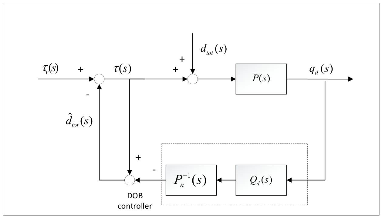
Here, d_res denotes the residual disturbance after DOB compensation. When $Q(s)$ ≈ 1, within the effective observation bandwidth, the corresponding disturbance component is attenuated, and the compensated plant approaches the local nominal dynamics defined in Section 3.2. The DOB structure is shown in Figure 1.

The actual plant P(s) is driven by the compensated control input, while the equivalent lumped disturbance d_tot(s) is estimated through the nominal inverse model P⁻¹_n(s) and the Q-filter. The estimated disturbance ${\widehat{d}}_{tot}(s)$ is fed back for disturbance compensation.

3.4. Filter Parameter Constraints and Robustness Analysis Based on the Small-Gain Theorem

The DOB observation bandwidth is constrained by unmodeled high-frequency dynamics and measurement noise. Accordingly, the Q-filter is selected using a small-gain robustness condition. A second-order binomial filter is adopted as

$$Q\left(s\right)={\displaystyle \frac{1}{{\left(\lambda s+1\right)}^2}}={\displaystyle \frac{1}{{\lambda }^2{s}^2+2\lambda s+1}}$$

(32)

where $\lambda$ is the filter time constant; decreasing $\lambda$ increases the effective observation bandwidth but also increases sensitivity to measurement noise and unmodeled high-frequency dynamics.

To evaluate the robustness of the DOB inner loop, the multiplicative model uncertainty between the actual plant and the nominal model is defined as

$$\Delta \left(s\right)={\displaystyle \frac{P\left(s\right)-P_n\left(s\right)}{P_n\left(s\right)}}$$

(33)

where P(s) is the transfer function of the actual manipulator plant, P_n(s) is the nominal plant used in the DOB design, and Δ(s) represents normalized model uncertainty. This uncertainty includes the effects of parameter mismatch, neglected flexible modes, unmodeled high-frequency dynamics, and digital implementation delay.

According to the small-gain theorem, a sufficient condition for robust internal stability of the DOB inner loop is

$$\left|\Delta \left(j\omega \right)Q\left(j\omega \right)\right|<1$$

(34)

For the prescribed plant set, the corresponding worst-case uncertainty bound is defined as

$${\Delta }_{\max }(\omega )={\max }_{\mathcal{P}}|\Delta (j\omega )|$$

(35)

where ${\max }_{\mathcal{P}}$ denotes the set of plants generated by the considered joint configurations, payload variations, parameter perturbations, and implementation conditions. Thus, a conservative Q-filter selection should satisfy

$$Q(j\omega )|<{\displaystyle \frac{1}{{\Delta }_{max}}}$$

(36)

at every considered frequency. For the second-order binomial Q-filter adopted in this study, Q(s), its frequency-response magnitude is

$$\left|Q\left(j\omega \right)\right|={\displaystyle \frac{1}{1+{\left(\lambda \omega \right)}^2}}$$

(37)

Substituting Equation (37) into Equation (36) yields

$${\displaystyle \frac{1}{1+{\left(\lambda \omega \right)}^2}}<{\displaystyle \frac{1}{{\Delta }_{\mathrm{m}\mathrm{a}\mathrm{x}}\left(\omega \right)}}$$

(38)

When ${\Delta }_{\max }(\omega )$ > 1, the corresponding lower bound of the filter time constant is

$$\lambda >{\displaystyle \frac{\sqrt{{\Delta }_{\mathrm{m}\mathrm{a}\mathrm{x}}\left(\omega \right)-1}}{\omega }}$$

(39)

Accordingly, $\lambda$ is selected above the maximum lower bound obtained from Equation (39), with an additional robustness margin. The resulting condition applies to the prescribed uncertainty set and does not imply robust stability for arbitrary unmodeled dynamics, payloads, or operating conditions outside the considered range.

$$P\left(s\right)=P_n\left(s\right)\left[1+\Delta \left(s\right)\right]$$

(40)

where P(s) denotes the actual manipulator plant, P_n(s) denotes the nominal plant used in the DOB design, and Δ(s) denotes the multiplicative uncertainty. For the DOB inner loop, a sufficient small-gain condition for robust internal stability is

$${\left|\left|Q\left(s\right)\Delta \left(s\right)\right|\right|}_{\infty }<1$$

(41)

or, equivalently,

$$\left|Q\left(j\omega \right)\Delta \left(j\omega \right)\right|<1$$

(42)

Since the exact uncertainty is not known for all operating conditions, the worst-case uncertainty bound is introduced as

$$\Delta \left(\omega \right)=max\left|\Delta \left(j\omega \right)\right|$$

(43)

$$\left|Q\left(j\omega \right)\right|\Delta \left(\omega \right)<1$$

(44)

over the considered frequency range. For the second-order binomial Q-filter adopted in this study, $Q(s)=1/{(\lambda s+1)}^2$, its frequency-response magnitude is $|Q(j\omega )|=1/[1+{(\lambda \omega )}^2]$. Thus, the sufficient robustness condition becomes $\Delta (\omega )/[1+{(\lambda \omega )}^2]<1$. When $\Delta \left(\omega \right)$ > 1, this inequality gives the lower bound of the filter time constant as

$$\lambda >sqrt\left[\Delta \left(\omega \right)-1\right]/\omega$$

(45)

In implementation, λ is selected above the maximum lower bound obtained from the considered frequency range with an additional robustness margin. Under this condition, the DOB satisfies the small-gain requirement within the prescribed uncertainty set, while high-frequency unmodeled dynamics, measurement noise, and neglected flexible modes remain as bounded residual uncertainties outside the effective observation bandwidth.

3.5. Outer-Loop Active Vibration Suppression Based on Eigenstructure Assignment

PESA is synthesized on a controller-oriented reduced-order model rather than on the complete six-joint structural model. Based on the retained-mode selection described in Section 4.1, the controller states consist of one equivalent rigid-body coordinate $q_l$, one retained flexible modal coordinate ${\dot{q}}_l$, and their corresponding velocities. The reduced state is therefore defined as $x={[q_l,{\dot{q}}_l,q_d,{\dot{q}}_d]}^T$, resulting in the fourth-order local representation given in Equation (46). The retained flexible coordinate represents the low-frequency modal component selected for residual-vibration suppression, whereas the effects of the unretained higher-order modes are treated as residual flexible dynamics in the robustness analysis:

$$\dot{x}(t)=Ax(t)+B{u}_v(t)$$

(46)

$$y(t)=Cx(t)$$

(47)

Matrix A denotes the reduced-order state matrix, and matrix B represents the input matrix associated with the outer-loop virtual control input. Since the DOB compensates for lumped disturbances and provides a nominalized model, PESA treats the outer-loop input as a virtual excitation applied to the reduced-order system. The matrices A and B are obtained by projecting the nominal rigid–flexible dynamics onto the retained modal subspace, including the equivalent inertia, modal stiffness, damping, and modal input mapping.

Because these parameters vary with manipulator configuration, A and B are posture-dependent. Therefore, the reduced-order matrices are calculated offline at representative scheduling postures, and the corresponding PESA gains are stored in the lookup table. The unretained higher-order modes are considered as residual flexible dynamics in the robustness analysis.

The fourth-order model is used for dominant-mode PESA synthesis rather than representing the complete six-joint flexible dynamics. The retained eigenvector subspace defines the modal direction for eigenstructure assignment, enabling selective modification of the targeted flexible modes. The eigen decomposition of the reduced-order system matrix is given as

$$A{v}_i={\lambda }_i{v}_i,\hspace{1em}i=1,\dots ,4$$

(48)

$$Vr=span\{vi,i\in Ir\}$$

(49)

$$Vf=span\{vi,\in If\}$$

(50)

where Ir and If denote the index sets of the retained rigid-body and flexible modes, respectively. The revised modal partition is not determined by a single natural-frequency threshold. Instead, the retained flexible-mode set is defined according to the modal analysis and the control objective, including the relevant natural frequencies, modal damping requirement, deformation distribution, and coupling with the targeted vibration direction. In the subsequent PESA design, damping is imposed explicitly through the desired closed-loop pole locations and target modal damping ratio rather than through a frequency-only classification criterion.

The rigid-body subspace Vr is retained explicitly because the objective of PESA is selective eigenstructure modification rather than full-state pole reassignment. The eigenstructure associated with the retained flexible subspace Vf is modified to increase modal damping, whereas the eigenstructure associated with Vr is preserved so that the baseline rigid-body trajectory-tracking dynamics are not intentionally altered by the vibration controller. Thus, Vr serves as the preservation constraint in the partial eigenstructure-assignment problem.

Since the system matrix A is structurally symmetric in the decoupled coordinate system, the eigenvectors corresponding to different modes satisfy the generalized orthogonality property, i.e., $V_r^T{V}_v=0$. This ensures that the configuration of ${\mathrm{\Lambda }}_v$ does not mathematically interfere with the characteristics of ${\mathrm{\Lambda }}_r$. A full-state feedback control law, $u_v=-Kx$, is designed so that the closed-loop system matrix $A_c=A-BK$ satisfies specific spectral configuration requirements: ${\mathrm{\Lambda }}_r$ remains unchanged, while ${\mathrm{\Lambda }}_v$ is moved to a high-damping region. For each desired closed-loop eigenvalue ${\lambda }_i^{closed}$, the following algebraic constraint is satisfied:

$$[{\lambda }_{i}I-A]v_i=B{w}_i$$

(51)

Equation (51) is rewritten in matrix form:

$$[{\lambda }_{i}I-A\hspace{1em}B]\left[\begin{array}{c}{v}_i\\ w_i\end{array}\right]=0$$

(52)

Define matrix $S({\lambda }_i)=[{\lambda }_{i}I-A\hspace{1em}B]$. For each desired eigenvalue ${\lambda }_i$, compute the null space basis $N_i$ of $S({\lambda }_i)$ as follows:

$$N_i=\mathrm{null}(S({\lambda }_i))=\left[\begin{array}{c}{U}_i\\ Z_i\end{array}\right]$$

(53)

where $U_i$ is the feasible space of the eigenvector, and $Z_i$ is the feasible space of the input vector. This means that any closed-loop eigenvector $v_i$ must be a linear combination of the column vectors $U_i$. For rigid-body modes, the open-loop eigenvector is directly selected as the closed-loop eigenvector, i.e., $v_r=v_r^{open}$. The corresponding input vector must be $w_r=0$. For vibration modes, $v_v$ is selected in the $U_v$ space to minimize the feedback gain norm or to satisfy specific decoupling conditions. Finally, the modal matrix $V=[v_{r1},v_{r2},v_{v1},v_{v2}]$ and the input matrix $W=[0,0,w_{v1},w_{v2}]$ are assembled. If $V$ is nonsingular, the feedback gain matrix $K$ is uniquely determined as $K=-W{V}^{-1}$.

To provide a clearer theoretical justification of the DOB–PESA closed-loop system, the stability analysis is reorganized as follows. The closed-loop system after DOB compensation and PESA feedback can be written as

$$\dot{x}=(\mathbf{A}-\mathbf{B}\mathbf{K})x+\mathbf{B}{d}_{res}$$

(54)

where A and B are the reduced-order state matrix and input matrix used for PESA synthesis, K is the PESA feedback gain, and $d_{res}$ denotes the residual disturbance after DOB compensation. When the DOB compensation is ideal within the effective bandwidth of the Q-filter, $d_{res}$ approaches zero, and Equation (54) reduces to the nominal closed-loop system. Therefore, the disturbance-free closed-loop form corresponds to the nominal compensated system $\dot{x}=(\mathbf{A}-\mathbf{B}\mathbf{K})x$, while the revised expression explicitly retains the DOB residual disturbance term.

The following assumptions are introduced for the stability analysis. The manipulator operates within the prescribed workspace and payload range used for nominal modeling and controller design. Second, the retained dominant flexible modes are controllable and observable in the reduced-order model. Third, the multiplicative uncertainty satisfies the small-gain condition of the DOB inner loop. Fourth, the residual disturbance after DOB compensation is bounded, namely $\left|\left|d_{res}\left(t\right)\right|\right| \le d_{bar}$.

For the nominal compensated system, the PESA feedback gain K is designed such that the selected flexible-mode poles are placed in the open left-half complex plane, while the retained rigid-body dynamics remain stable under the baseline tracking loop. Therefore, the nominal closed-loop matrix is defined as ${\mathbf{A}}_{\mathrm{c}}=\mathbf{A}-\mathbf{B}\mathbf{K}$, and ${\mathbf{A}}_{\mathrm{c}}$ is Hurwitz. For any positive definite matrix $\mathbf{W}={\mathbf{W}}^T>0$, there exists a unique symmetric positive-definite matrix $\mathbf{P}={\mathbf{P}}^T>0$ satisfying the Lyapunov equation:

$${\mathbf{A}}_c^T\mathbf{P}+\mathbf{P}{\mathbf{A}}_c=-\mathbf{W}$$

(55)

Choose the Lyapunov function:

$$V=x^T\mathbf{P}x$$

(56)

Since P is positive definite, V(x) is positive definite. Along the trajectory of the nominal compensated system, the derivative of V(x) is

$$\dot{V}=x^T(A_c^{T}P+P{A}_c)x=-x^T{Q}_{L}x<0$$

(57)

Thus, the nominal DOB–PESA closed-loop system is asymptotically stable.

For the actual system, the DOB residual disturbance and unmodeled dynamics are not assumed to be zero. With the bounded residual disturbance $\left|\left|d_{res}\left(t\right)\right|\right|\le d$, the derivative of the Lyapunov function satisfies

$$\dot{V}=-x^T\mathbf{W}x+2x^T\mathbf{P}\mathbf{B}{d}_{res}$$

(58)

Assume that the DOB residual disturbance is bounded, namely $\Vert d_{res}\Vert \le \overline{d}$, where $\overline{d}>0$ is the upper bound of the residual disturbance. Then, the derivative of the Lyapunov function satisfies $\dot{V}\le -{\lambda }_{min}(W)\parallel x{\parallel }^2+2\parallel PB\parallel \overline{d}\parallel x\parallel$. The first term on the right-hand side is a negative quadratic term, while the second term is caused by the bounded DOB residual disturbance. When the state norm is larger than $||x||>{\displaystyle \frac{2|PB|\overline{d}}{{\lambda }_{\min }(W)}}$, the negative quadratic term dominates the residual-disturbance term. Therefore, $\dot{V}<0$ is guaranteed outside this bounded neighborhood. This indicates that the closed-loop state will converge toward and remain within a bounded neighborhood of the equilibrium point. Hence, under a bounded DOB residual disturbance, the actual DOB–PESA closed-loop system is uniformly ultimately bounded in the standard Lyapunov sense [32].

It should be noted that, inside this bounded neighborhood, the upper-bound estimate of $\dot{V}$ may become nonnegative. However, this does not mean that the actual value of $\dot{V}$ must be positive. It only means that strict negativity of $\dot{V}$ cannot be guaranteed by this upper-bound estimate in that region.

In the nominal compensated case, the residual disturbance is zero, namely $d_{\mathrm{res}}=0$. Then, Equation (57) becomes $\dot{V}=-x^{T}Wx<0$. Therefore, the nominal DOB–PESA closed-loop system is asymptotically stable.

According to the DOB robustness analysis in Section 3.4, the Q-filter satisfies the small-gain condition within the prescribed uncertainty range, ensuring bounded DOB residual disturbances and stable inner-loop compensation.

For gain scheduling, the PESA gains are computed offline at representative scheduling points, where the corresponding closed-loop matrices are verified to be Hurwitz. During online operation, the gains are updated through interpolation within the prescribed scheduling range, preserving local stability over the considered operating conditions.

The state vector $x(t)$ at any time can be expressed as a linear combination of the closed-loop eigenvectors:

$$x(t)={\displaystyle \sum _{j\in \{r1,r2\}}{c}_j}{e}^{{\lambda }_{j}t}{v}_j+{\displaystyle \sum _{k\in \{v1,v2\}}{c}_k}{e}^{{\lambda }_{k}t}{v}_k$$

(59)

This section presents the modal decomposition of the feedback control input. The control input $u_v(t)=-Kx(t)$ can also be decomposed into modal components:

$$u_v(t)=-Kx(t)=-{\displaystyle \sum c_j}{e}^{{\lambda }_{j}t}K{v}_j-{\displaystyle \sum c_k}{e}^{{\lambda }_{k}t}K{v}_k$$

(60)

For rigid-body modes, the input coupling vector $w_j=0$ is explicitly constrained. According to the relation $w_j=-K{v}_j$, we obtain $\mathrm{Term} \mathrm{A}=K{v}_j=0$. When the system undergoes only rigid-body motion, $x$ lies entirely in the subspace $V_r$. In this case, the feedback torque is zero. For an ideal state component lying entirely in the retained rigid-body subspace, the PESA feedback contribution associated with the flexible-mode channel is zero by construction. The controller is therefore designed not to intentionally relocate the retained rigid-body eigenstructure, while practical coupling and modeling uncertainty remain subject to the robustness analysis. For the vibration mode $k\in \{v1,v2\}$, the term $\mathrm{Term} \mathrm{B}=K{v}_k\ne 0$ appears. This means that once the sensor detects that the state variable contains flexible modal components, the controller will immediately generate an opposite suppression torque, achieving precise vibration suppression.

The modal decomposition enables PESA to selectively modify flexible-mode dynamics without uniformly increasing the position-loop gain. The rigid-body modes associated with trajectory tracking are preserved, while the selected flexible-mode poles are shifted toward higher damping, resulting in faster vibration decay with limited influence on tracking performance.

3.6. Gain Scheduling Mechanism

To compensate for pose-dependent modal-frequency variation, a joint-pose-driven gain scheduling mechanism is introduced to update the PESA feedback gain according to the current manipulator configuration.

The scheduling variables are selected according to the sensitivity of the dominant modal frequencies to joint-angle variation. For the r-th dominant flexible mode, the frequency sensitivity with respect to the i-th joint angle is evaluated by

$$S_i^{(r)}=|f_r(q)/q_i|$$

(61)

where $f_r(q)$ denotes the r-th modal frequency at configuration q. In implementation, the derivative is calculated using finite differences at representative operating postures. To compare the overall influence of each joint on the retained dominant modes, the normalized sensitivity index is defined as

$${\mathrm{\Gamma }}_i={\displaystyle \frac{{\displaystyle \sum _{r=1}^{N_m}{S}_i^{(r)}}}{{\displaystyle \sum _{j=1}^6{\displaystyle \sum _{r=1}^{N_m}{S}_j^{(r)}}}}}$$

(62)

where N_m is the number of retained flexible modes and ${\mathrm{\Gamma }}_i$ denotes the normalized modal-frequency sensitivity associated with the i-th joint. The index is used as a relative screening criterion for scheduling-variable selection rather than as an independent controller-performance metric. A larger ${\mathrm{\Gamma }}_i$ indicates a stronger influence of the corresponding joint-angle variation on the retained modal frequencies.

The sensitivity screening identifies Joint 2 and Joint 3 as the primary scheduling variables within the considered posture set. This selection is also consistent with the manipulator geometry: Joint 2 and Joint 3 correspond to the shoulder and elbow axes, whose variations directly modify the manipulator configuration, effective inertia distribution, and flexible-mode characteristics. Joint 1 mainly changes the base azimuth, whereas Joints 4–6 primarily modify the wrist orientation with shorter effective moment arms. Accordingly, q₂ and q₃ are used to parameterize the offline PESA gain schedule, while the influence of the remaining joints is included in the residual model uncertainty.

The system adopts an offline computation combined with an online lookup table scheduling strategy. In the offline stage, the controller design is completed in advance for typical joint configurations, and the feedback gain matrix is generated. In the online stage, the current gain is obtained in real time through simple interpolation lookup:

$$u(t)=-{\widehat{d}}_{tot}(t)-K(q_s)x(t)$$

(63)

Equation (63) is the composite control law for the entire system, where $K(q_s)$ is the pose feedback matrix. During online operation, linear interpolation is performed between adjacent feature points based on the current joint angle $q_s$ to calculate the currently required feedback gain matrix:

$$K(q_s)={\displaystyle \sum _{i=1}^N{w}_i}(q_s)K_i$$

(64)

where $K_i$ denotes the offline preset gain matrix at the i-th pose. The weight $w_i(q_s)$ is determined according to the inverse Euclidean distance between the current configuration and the preset pose points, where N represents the total number of scheduling points. The interpolation-based gain update provides a smooth transition between neighboring PESA gains during configuration changes.

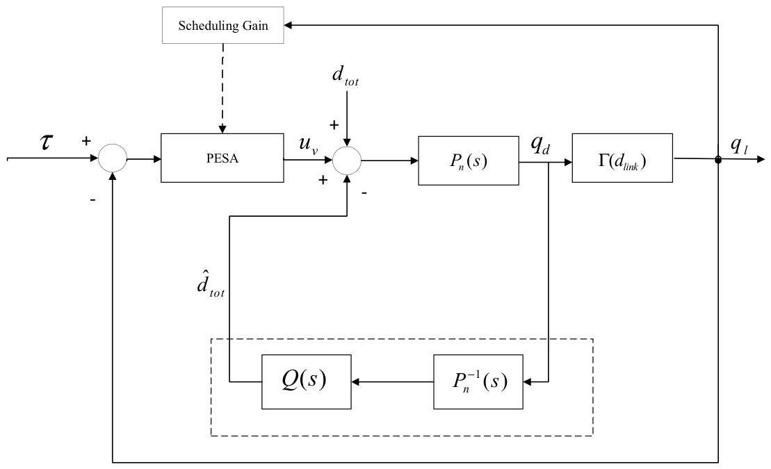
The operator $\mathrm{\Gamma }(d_{link})$ in Equation (24) represents the mapping of link-side disturbances to the motor-side equivalent disturbance through the flexible-joint dynamics. The DOB estimates and compensates for this equivalent disturbance, thereby reducing the influence of external disturbances on the motor-side dynamics. Figure 2 illustrates the overall DOB–PESA composite control framework with modal scheduling.

The DOB provides disturbance compensation, while the PESA layer generates the modal-feedback input and the scheduling mechanism updates the PESA gain according to manipulator configuration. For implementation, the PESA gains are calculated offline at representative scheduling points, where the corresponding closed-loop matrices are verified to be Hurwitz. During operation, the gain is obtained by interpolation within the prescribed scheduling range, preserving local closed-loop stability over the validated configurations. This conclusion is limited to the considered scheduling range and does not imply global stability for arbitrary configurations.

4. Simulation and Experimental Verification

To verify the effectiveness of the proposed vibration-suppression framework, numerical simulation and real-manipulator measured-data validation are conducted. The numerical evaluation compares PID, standalone DOB, standalone PESA, and the proposed DOB–PESA controller, with an additional fixed-gain versus scheduled-gain comparison to assess the contribution of gain scheduling.

Section 4.1, Section 4.2, Section 4.3 and Section 4.4 present numerical validation based on the simplified rigid-link flexible-joint model of the Aubo i5 manipulator (Aubo (Beijing) Intelligent Technology Co., Ltd., Beijing, China) under identical reference inputs, payload, disturbance conditions, sampling settings, actuator constraints, and initial conditions. Modal analysis identifies the first two flexible modes at 41.837 Hz and 42.029 Hz as the dominant residual-vibration modes, which are retained for the reduced-order PESA design. The controller parameters remain consistent among corresponding comparison cases to ensure a fair evaluation.

Section 4.5 further validates the proposed framework using 16-channel measured operating-condition data collected from the Aubo i5 manipulator.

4.1. Simulation-Based Modal Analysis of the Manipulator

Modal analysis is performed on the simplified Aubo i5 structural model to obtain the natural frequencies and mode shapes for identifying the dominant flexible dynamics used in controller design. To improve computational efficiency, geometric details and joint connections are simplified, with joint interfaces represented by equivalent axial and surface contacts. The main structural components are modeled using 6061 aluminum alloy, and the masses of non-structural components, including servo motors and electrical elements, are equivalently assigned to the corresponding joints.

A 10 kg vertical payload is applied at the end-effector under the representative reference posture used for controller-oriented model construction. The first six natural frequencies and corresponding deformation characteristics obtained from the modal analysis are summarized in

Table 1. First six natural frequencies and deformations of vibration under classic operating poses.

Order	Natural Frequency/Hz	Maximum Deformation/mm	Location of Maximum Deformation
First-order vibration	41.837	11.28	Sixth joint
Second-order vibration	42.029	11.367	Sixth joint
Third-order vibration	196.76	17.119	Sixth joint
Fourth-order vibration	212.32	14.554	Sixth joint
Fifth-order vibration	278.45	13.587	Fifth joint
Sixth-order vibration	338.93	8.025	Third joint

.

The modal characteristics in Table 1 define the retained modal subspace for PESA design. Mode selection considers both natural frequency and deformation distribution. Although the third and fourth modes exhibit larger deformation magnitudes, their higher frequencies make them less critical under the considered operating conditions. Therefore, the first two modes at 41.837 Hz and 42.029 Hz are selected as the retained flexible modes because their deformation is concentrated near the sixth joint, where the end-effector is mounted. The higher-order modes are treated as residual flexible dynamics in the robustness analysis.

Based on these retained modes, PESA is designed using a fourth-order reduced-order model consisting of one rigid-body coordinate and one flexible modal coordinate with their corresponding velocity states. This reduction preserves the dominant vibration characteristics while maintaining controller implementation efficiency. The structural model also provides the configuration information for selecting q2 and q3 as scheduling variables in Section 3.6.

Figure 3 shows the deformation distribution obtained from modal analysis at the selected operating posture, illustrating the spatial characteristics of the retained flexible response.

The deformation contour provides spatial modal information for retained-mode assessment and modal projection rather than a direct controller model. The reduced-order PESA model is therefore established for low-frequency residual-vibration suppression rather than reproducing the complete modal response of the manipulator.

Although the third and fourth modes exhibit larger deformation magnitudes, their higher frequencies make them less critical under the considered operating conditions. The first two modes at 41.837 Hz and 42.029 Hz are retained because they combine relatively low frequencies with deformation concentrated at the sixth joint, where the end-effector is mounted. Therefore, the mode selection considers both frequency characteristics and deformation distribution, while higher-order modes are treated as residual flexible dynamics in the robustness analysis.

The retained modes are interpreted as controller-oriented low-frequency modes rather than experimentally confirmed global dominant modes, since independent modal participation identification was not performed. The higher-frequency modal variations used in the gain-scheduling study are only adopted to evaluate frequency-drift adaptation.

4.2. Comparative Simulation of Step Responses

A unit step command is applied to each joint to compare PID, standalone DOB, standalone PESA, and DOB–PESA under identical rigid–flexible model, reference input, payload, disturbance, sampling, actuator constraints, and initial conditions. Since the controller structures differ, the parameters are selected according to their respective design principles rather than identical numerical gains.

The PID controller is used as the baseline, with gains Kp = [420,450,380,240,160,120], Ki = [35,38,30,20,12,10], and Kd = [30,32,27,18,12,9] for Joints 1–6. The same PID gains are retained when DOB is introduced. The DOB Q-filter is selected according to the small-gain condition in Section 3.4 as Q(s) = 1/(0.005s + 1)2, with λ = 0.005s and a cutoff frequency of 31.83 Hz.

The PESA gain is designed using the reduced-order modal model with the first two flexible modes (41.837 Hz and 42.029 Hz), desired damping ratio ζd = 0.707, and closed-loop poles (−185.85 ± 185.90j) and (−186.70 ± 186.76j). The same PESA parameters are used in standalone PESA and DOB–PESA to avoid case-specific retuning.

Figure 4a–f show the responses. PID exhibits larger oscillations, while DOB and PESA provide partial vibration reduction through disturbance compensation and modal damping, respectively. The proposed DOB–PESA controller achieves faster convergence and lower residual oscillation across all joints.

4.3. Simulation of End-Effector Residual Vibration Suppression

Residual vibration may occur during high-speed positioning and sudden stopping due to flexible-joint dynamics, inertial effects, and unmodeled disturbances. In this experiment, the four control strategies are evaluated under transient operating conditions to compare their vibration attenuation and settling performance. Figure 5 shows the simulated end-effector residual-vibration responses.

As shown in Figure 5, an impact disturbance is introduced at 0.4 s to evaluate transient vibration attenuation. The PID controller exhibits the largest oscillation, while standalone DOB and PESA reduce vibration through disturbance compensation and modal damping, respectively, but residual oscillations remain. In comparison, the DOB–PESA controller achieves smaller displacement deviation and faster residual-vibration decay, especially for the vibration-sensitive end joints (Joints 4–6).

Figure 6 further evaluates end-effector residual vibration under simulated high-speed motion and emergency-stop conditions in the X, Y, and Z directions. The motion starts at 0.1 s, and the emergency stop occurs at 1 s.

During Cartesian motion along the X, Y, and Z directions, inertial impacts occur during start-up and emergency stopping. As shown in Figure 6, the PID controller exhibits the largest residual vibration after the 1 s emergency stop. The standalone DOB reduces sustained oscillation but retains an instantaneous vibration peak. In comparison, the DOB–PESA controller achieves smaller deviation and faster recovery in all three directions, demonstrating improved transient vibration attenuation.

4.4. Simulation Verification of Gain Scheduling Under Representative Modal Frequencies

To evaluate the adaptability of the gain-scheduling mechanism to pose-dependent modal-frequency variation, a sensitivity test is conducted using a simplified second-order flexible-mode model. The representative frequencies of 280, 300, and 320 Hz are selected as scheduling points for different stiffness conditions. The 280 Hz point is obtained by rounding the fifth-order frequency of 278.45 Hz, 300 Hz is selected as the nominal design frequency, and 320 Hz represents an increased stiffness condition within the fifth- and sixth-order modal interval.

The fixed-gain controller is designed at 300 Hz, while the scheduled-gain controller updates the PESA feedback gain according to the representative frequency. The target damping ratio is set to 0.707 for all cases. The scheduling frequencies are generated by varying q2 and q3 while keeping other joint angles at nominal values to isolate the stiffness variation associated with the shoulder–elbow configuration.

As the Figure 7 show, the fixed-gain controller shows degraded transient performance when the modal frequency deviates from the nominal 300 Hz design point. At 280 Hz, the overshoot increases to 8.2% and the settling time increases to 0.38 s, while the response at 320 Hz also differs from the nominal condition. In contrast, the scheduled-gain controller maintains an overshoot below 5% and a settling time below 0.30 s over all tested frequencies, demonstrating improved adaptability to stiffness-dependent modal-frequency variations.

Table 2. Comparison of end-effector gain performance.

Stiffness Condition	Frequency (Hz)	Control Strategy	Rise Time (s)	Overshoot (%)	Settling Time (s)
Low stiffness	280	Fixed gain	0.15	8.2	0.38
		Scheduled gain	0.10	4.5	0.26
Medium stiffness	300	Fixed gain	0.12	4.1	0.29
		Scheduled gain	0.12	4.1	0.29
High stiffness	320	Fixed gain	0.09	1.8	0.24
		Scheduled gain	0.09	1.2	0.18

summarizes the corresponding end-effector step-response indicators.

4.5. Real-Manipulator Hardware Validation Using Directly Measured 16-Channel Responses

These results evaluate the lookup-table scheduling strategy described in Section 3.6. At the nominal 300 Hz condition, the fixed-gain and scheduled-gain controllers show identical responses because the nominal stored gain is used. When the modal frequency shifts to 280 Hz, the scheduled controller reduces the rise time from 0.15 s to 0.10 s, overshoot from 8.2% to 4.5%, and settling time from 0.38 s to 0.26 s. At 320 Hz, the overshoot decreases from 1.8% to 1.2% and the settling time from 0.24 s to 0.18 s. These results demonstrate that gain interpolation improves transient consistency under modal-frequency variations.

To further validate the proposed vibration-suppression framework, hardware tests were conducted on an Aubo i5 industrial manipulator using a representative 13 s operating trajectory. The PID, standalone DOB, standalone PESA, and DOB–PESA controllers were implemented separately, and the corresponding 16-channel acceleration responses were directly measured. The measured signals are expressed in m/s² and represent the physical vibration responses under each control condition.

The 16-channel measurement system consists of five tri-axial accelerometers and one single-axis accelerometer. The tri-axial sensors are installed at five joint locations and provide 15 acceleration channels along three orthogonal directions, while the additional single-axis sensor is installed at the base and measures vertical acceleration. Therefore, Figure 8 presents distributed multi-location acceleration responses rather than 16 measurements of a single end-effector acceleration component.

Figure 8 presents measured closed-loop hardware responses obtained during controller execution rather than offline-processed controller outputs. The comparison reflects the vibration differences produced by the PID, standalone DOB, standalone PESA, and DOB–PESA configurations under the same operating task.

In accordance with Section 2.3, x(t) denotes the acceleration time history of an individual measurement channel used for modal-feature analysis.

The results evaluate the lookup-table scheduling strategy described in Section 3.6. At the nominal 300 Hz condition, the fixed-gain and scheduled-gain controllers show identical responses. When the frequency changes to 280 Hz, the scheduled controller reduces the rise time from 0.15 s to 0.10 s, overshoot from 8.2% to 4.5%, and settling time from 0.38 s to 0.26 s. At 320 Hz, the overshoot decreases from 1.8% to 1.2% and the settling time from 0.24 s to 0.18 s, demonstrating improved transient consistency under modal-frequency variation.

Hardware validation was conducted on an Aubo i5 manipulator using a representative 13 s operating trajectory. The PID, DOB, PESA, and DOB–PESA controllers were implemented separately, and the corresponding 16-channel acceleration responses were directly measured. The measurement system consists of five tri-axial accelerometers installed at joint locations and one single-axis accelerometer at the base, providing distributed multi-location vibration responses rather than a single end-effector measurement.

Figure 8 presents the measured closed-loop responses during controller execution. The signal x(t) denotes the acceleration time history of an individual measurement channel used for modal-feature analysis.

5. Conclusions

This study develops a composite vibration-suppression framework integrating a disturbance observer (DOB), partial eigenstructure assignment (PESA), and pose-dependent gain scheduling for a rigid–flexible Aubo i5 industrial manipulator. A local rigid–flexible nominal model with lumped disturbances is established for controller synthesis. The DOB provides disturbance compensation under the small-gain robustness constraint, the PESA controller selectively increases the damping of retained flexible modes while preserving rigid-body dynamics, and the gain-scheduling mechanism updates modal feedback gains according to configuration-dependent frequency variation.

The numerical results verify the individual and combined contributions of the proposed control components. Compared with PID, standalone DOB, and standalone PESA controllers, the proposed DOB–PESA controller achieves faster transient convergence, reaching the target with negligible residual oscillation within approximately 0.3 s. Under impact disturbance, the principal residual vibration is suppressed within approximately 0.1 s. The fixed-gain and scheduled-gain comparison further demonstrates that the scheduling mechanism maintains a settling time below 0.30 s and an overshoot below 5% under the tested modal-frequency variations.

Hardware experiments were conducted on the physical Aubo i5 manipulator using a representative 13 s operating trajectory with directly measured 16-channel acceleration responses. Under the considered operating condition, the proposed controller reduces the dominant low-frequency vibration amplitude by approximately 80% compared with the PID baseline and suppresses most residual vibration within approximately 1 s. These results demonstrate the effectiveness of the coordinated DOB–PESA framework for disturbance rejection and flexible-mode attenuation under the tested conditions.

The conclusions are limited to the investigated models, representative modal-frequency conditions, and Aubo i5 experiments. Broader validation involving additional payloads, workspace configurations, longer-duration tasks, and independent experimental modal identification will be considered in future work.