A Phase-Aware Prediction-Horizon Policy for Learned-Cost CEM-MPC Lane-Change Planning

Abstract

Model Predictive Control (MPC) offers a structured approach for autonomous-vehicle motion planning by optimizing predicted vehicle behavior over a finite horizon. As learning-based components become increasingly integrated into autonomous systems, interpretable interfaces between decision-making and control become increasingly important. Motivated by the need to examine how predictive depth should vary with maneuver context, this paper proposes and evaluates an adaptive phase-aware horizon-selection formulation within a hybrid Maximum Entropy Deep Inverse Reinforcement Learning-Model Predictive Control (MEDIRL-MPC) framework. The formulation conditions prediction depth explicitly on the recognized maneuver phase, providing an interpretable scheduling signal rather than maintaining the horizon as a globally fixed controller parameter. The considered architecture combines a MEDIRL-informed driving cost, a sampling-based Cross-Entropy Method planner, a kinematic vehicle model, and a scenario manager that identifies the current lane-change phase and provides the corresponding reference information. Controlled experiments are conducted in the CARLA simulator using a static-obstacle lane-change scenario. Fixed-horizon baselines, phase-wise analysis, common-state counterfactual comparisons, and controlled robustness experiments are used to evaluate the effect of prediction depth. The results indicate that the prediction horizon length greatly affects closed-loop behavior and computational demand, and that the relative suitability of different horizons varies across each scenario phase. The phase-aware policy further demonstrates that predictive depth can be allocated selectively across maneuver phases while preserving successful maneuver execution, and remains successful and lane-safe under controlled variations in target speed, obstacle distance, and activation distance. These findings support maneuver phase as an interpretable context for prediction-horizon adaptation within the evaluated architecture, while limiting the conclusions to the investigated scenario and experimental setting.

1. Introduction

Model Predictive Control (MPC) has become an established framework for autonomous-vehicle motion planning and control because it explicitly evaluates the future consequences of candidate control actions over a finite prediction horizon. By repeatedly solving a constrained optimization problem using the latest vehicle state, MPC can integrate trajectory tracking, collision avoidance, actuator limitations, passenger comfort, and computational requirements within a unified decision-making process. Its performance, however, depends strongly on the configuration of the underlying predictive problem, including the length of the prediction horizon [1]. As learning-based components enter autonomous-driving pipelines, understanding how they influence planning decisions becomes more difficult, which motivates architectures in which adaptation remains explicit and interpretable.

The prediction horizon determines how far into the future the planner evaluates the evolution of the vehicle and its environment. A sufficiently long horizon may improve anticipation of upcoming obstacles, road geometry, and interactions with surrounding vehicles. It may also enable the planner to initiate a maneuver early enough to avoid aggressive or infeasible corrective actions. Increasing the horizon nevertheless enlarges the optimization problem and may considerably increase computation time, particularly in sampling-based MPC methods that propagate and evaluate numerous candidate control sequences [2]. Furthermore, information concerning the distant future may become progressively less reliable as prediction uncertainty and behavioral ambiguity increase with temporal distance [3,4]. A short horizon can reduce computational cost and concentrate the optimization on immediate control objectives, but it may provide insufficient foresight for safety-critical or interaction-dependent maneuvers. Therefore, prediction-horizon selection represents a fundamental trade-off between anticipatory capability, control quality, computational efficiency, and prediction reliability.

Most MPC implementations employ a fixed prediction horizon that remains unchanged throughout a maneuver. This design effectively allocates the same predictive depth to every control instant, despite changes in the local objective and decision context of the maneuver. A lane-change maneuver, however, is not a temporally uniform control task. During the approach phase, the planner must anticipate the obstacle or driving objective that motivates the maneuver and determine when lateral motion should begin. During the lane-transition phase, it must coordinate longitudinal and lateral motion while maintaining safe separation and producing a feasible trajectory [5]. During stabilization, the vehicle must converge smoothly to the target-lane reference without unnecessary steering oscillation or excessive computation. These phases differ in their immediate objectives, safety constraints, and requirements for anticipatory planning.

Adaptive- and variable-horizon MPC methods have attempted to address the limitations of fixed-horizon control by adjusting the prediction horizon according to variables such as vehicle speed, road curvature, lateral tracking error, environmental complexity, or computational load [6]. Other approaches modify the temporal discretization of the prediction interval [7] or employ optimization and learning methods to select an appropriate horizon. Although these studies establish that horizon adaptation can improve the balance between control performance and computational cost, the adaptation signal is commonly derived from continuous physical or numerical variables. The semantic progression of the maneuver, as an explicit and interpretable context for prediction-horizon selection, has been comparatively less explored.

This paper investigates whether the phase of an autonomous lane-change maneuver can be used to determine the predictive depth of an MPC planner. The central premise is that the most suitable horizon may not be globally constant but may depend on whether the vehicle is approaching the maneuver, transitioning between lanes, or stabilizing within the target lane. Accordingly, the prediction horizon is formulated as a function of a discrete maneuver-phase variable. This phase-aware formulation does not replace low-level state information or safety constraints; rather, it introduces maneuver phase as an explicit and interpretable context for allocating predictive effort.

The proposed formulation is considered within a learned-cost, sampling-based MPC architecture. In this architecture, a MEDIRL-informed driving cost represents behavioral preferences, with additional task-specific terms introduced for the lane-change scenario, while the MPC planner evaluates candidate control sequences over the selected horizon. This distinction is important: the learned cost specifies which predicted behaviors are desirable, whereas the horizon determines how far into the future their consequences are evaluated. Conditioning the horizon on maneuver phase therefore modifies the temporal scope of reasoning without changing the underlying behavioral objective.

Research Questions and Contributions

The study addresses the following research questions:

• RQ1: How does the prediction horizon affect the closed-loop behavior and computational requirements of learned-cost MPC during an autonomous lane-change maneuver?
• RQ2: Do the approach, lane-transition, and stabilization phases exhibit different horizon-performance relationships?
• RQ3: Can a phase-aware horizon policy provide a more favorable balance among maneuver success, safety, tracking quality, control smoothness, and planning time than a globally fixed horizon?
• RQ4: How robust is the phase-aware horizon policy to variations in vehicle speed, obstacle distance, and initial maneuver conditions?

The intended contributions of this work are as follows:

1.

A phase-aware formulation of prediction-horizon selection that represents the MPC horizon as a function of the semantic phase of an autonomous lane-change maneuver.

2.

The integration of phase-conditioned horizon selection into a learned-cost, sampling-based MPC planning architecture, in which behavioral preference and predictive depth remain separately defined and interpretable.

3.

A phase-wise evaluation methodology that complements conventional whole-maneuver metrics and reveals how horizon selection affects different stages of the maneuver.

4.

An experimental comparison between the proposed phase-aware policy and matched fixed-horizon baselines in a simulated obstacle-avoidance lane-change task.

The remainder of the paper is organized as follows. Section 2 reviews finite-horizon MPC, prediction-horizon adaptation, learned-cost planning, and maneuver-phase representations. Section 3 describes the proposed planning framework and its implementation. Section 4 presents the experimental protocol and evaluation metrics. Section 5 reports and discusses the results. Finally, Section 6 summarizes the main findings, identifies the limitations of the study, and outlines directions for future research.

2. Background and Related Work

2.1. Prediction Horizon in Model Predictive Control

MPC determines the current control action by optimizing predicted system behavior over a finite horizon. At each control instant, candidate control sequences are evaluated using a predictive model and an objective that may account for tracking accuracy, safety, comfort, and control constraints [8]. At each control instant t, MPC predicts the future evolution of the system over a finite prediction horizon N:

$$x_{t+k+1}=f(x_{t+k},u_{t+k}),k=0,\dots ,N-1,$$

(1)

and optimizes a sequence of future control inputs

$$U_t=\{u_t,u_{t+1},\dots ,u_{t+N-1}\}.$$

(2)

A standard finite-horizon objective can be written as

$$J_t(U_t;N)={\displaystyle \sum _{k=0}^{N-1}}\mathsf{\ell }(x_{t+k},u_{t+k})+V_f\left(x_{t+N}\right),$$

(3)

where $\mathsf{\ell }(·)$ denotes the stage cost and $V_f(·)$ denotes a terminal cost, when such a terminal term is included.

After solving the finite-horizon optimization problem, only the first control action is applied, and the problem is solved again at the next time step using the updated vehicle state. This receding-horizon mechanism allows MPC to react to updated state observations while still evaluating the predicted consequences of candidate control actions over a future interval. In autonomous-driving applications, this property is particularly attractive because the controller must simultaneously satisfy tracking, comfort, safety, and feasibility requirements in changing road and traffic conditions [9].

The prediction horizon N determines how far into the future the optimizer evaluates candidate actions. A longer horizon allows the planner to account for more distant road geometry, obstacles, traffic-light phases, or interaction effects, whereas a shorter horizon concentrates computation on near-term vehicle evolution [10]. However, increasing the prediction horizon also increases the number of predicted states, decision variables, constraints, and cost evaluations, creating a direct trade-off between foresight and real-time feasibility [7].

For sampling-based planners such as CEM–MPC or MPPI, computational effort is strongly influenced by the number of candidate control sequences, optimization iterations, and prediction steps, since each candidate must be propagated and evaluated through the predictive model over the selected horizon [2].

The relationship between horizon length and closed-loop performance is not necessarily monotonic. Extending the horizon may improve anticipation but might increase optimization dimensionality as also reliance on less certain distant predictions. Conversely, a short horizon may improve real-time responsiveness while providing insufficient foresight for upcoming obstacles, high-curvature road segments, or interaction-critical events [10,11]. Prediction-horizon selection therefore represents a trade-off among foresight, control performance, prediction reliability, and real-time feasibility.

2.2. Adaptive and Variable Horizon MPC

The term adaptive MPC should be used carefully because it can refer to different adaptation mechanisms. One common meaning is model adaptation, where the controller updates uncertain model parameters or robustness bounds online. For example, adaptive learning MPC for autonomous ground vehicles uses recursive parameter estimation to improve prediction accuracy under parametric and additive uncertainties while maintaining recursive feasibility and input-to-state stability under derived conditions [8]. Multi-model adaptive predictive control similarly updates the internal vehicle model to compensate for tire cornering-stiffness uncertainty, improving robustness without relying only on conservative worst-case design [12].

These model-adaptive approaches improve the fidelity of the prediction model, but they do not necessarily change the temporal depth of the prediction problem. In contrast, adaptive prediction-horizon methods modify how far the optimizer looks ahead, how the prediction interval is discretized, or how many future steps are included in the optimization [13].

Adaptive and variable-horizon methods can be distinguished by the information used to trigger adaptation and by whether adaptation modifies the number of prediction steps, their temporal spacing, or the overall prediction time.

One group of approaches adapts the prediction horizon using road geometry and vehicle-state variables. For example, fuzzy adaptive NMPC has been used to adjust the prediction horizon based on road curvature and vehicle speed, improving the balance between lateral tracking accuracy and solution time compared with fixed-horizon controllers [11]. Similarly, variable-prediction-horizon MPC methods have linked the horizon to vehicle speed, road curvature, lateral offset, steering frequency, or real-time performance indicators in order to improve path-tracking accuracy, comfort, and computational efficiency [14,15,16]. Dynamic-horizon MPC has also been proposed for trajectory tracking, where the prediction and control horizons are adjusted based on reference-trajectory curvature, vehicle speed, and lateral tracking error [17].

A second group uses optimization or learning mechanisms to select the horizon. Reinforcement-learning-based approaches, such as PPO-MPC, formulate the prediction horizon as an action selected according to vehicle state and path information, allowing the controller to adapt to different speeds and curvatures [13]. Other works use particle swarm optimization, neural networks, or fitted mappings to estimate suitable horizons or prediction times from performance data [14]. These methods automate horizon selection using observed vehicle, road, or performance variables, but the adaptation context remains primarily numerical rather than high-level maneuver semantics.

A third group modifies the temporal structure of the horizon rather than only changing the number of prediction steps. Time-varying and non-uniformly spaced MPC uses dense prediction intervals near the current state and sparse prediction intervals farther ahead, allowing the planner to preserve near-term control accuracy while extending the effective look-ahead range without a proportional increase in optimization size [7]. Variable-prediction-time MPC further coordinates the prediction horizon and the discretization interval, linking prediction time to path curvature, longitudinal speed, and tire–road friction in order to improve tracking performance without increasing computational burden [18]. Cycle-aware adaptive-horizon MPC applies a similar principle in signalized-intersection control by placing finer time steps near signal phase transitions and coarser steps farther away, thereby extending the effective prediction interval over traffic-signal cycles while maintaining a fixed number of optimization nodes [19].

A fourth direction uses the planning horizon as part of interaction-aware behavior. Negotiation-aware motion planning has shown that dynamically modifying the prediction horizon can change the planning modality in interactive driving scenarios, allowing the vehicle to respond differently to other agents during negotiation-like situations [20]. This line of work is relevant to the present study because it suggests that the horizon can influence the planner’s behavioral mode, rather than functioning only as a computational or tracking parameter.

Existing methods, therefore, condition horizon adaptation primarily on geometric, kinematic, dynamic, computational, or interaction-related variables. Explicitly conditioning predictive depth on the discrete progression of a maneuver remains comparatively less explored, particularly when maneuver phase is used as an interpretable planning context.

2.3. Learned-Cost MPC and Research Positioning

A separate challenge in MPC-based autonomous driving is the design of the objective function. Hand-designed MPC costs often require manual balancing of tracking accuracy, smoothness, safety, comfort, and efficiency, and the resulting behavior may be sensitive to the chosen weights [21]. Inverse Reinforcement Learning (IRL) addresses this difficulty by learning a reward or cost representation from expert demonstrations, allowing expert-like preferences to be embedded into downstream optimal-control or reinforcement-learning policies [22].

Learned-cost MPC has also been investigated in autonomous driving. Lee et al. demonstrated that a MEDIRL-learned spatiotemporal costmap can be consumed by MPC to perform lane keeping and lane changing in CARLA, reducing the need for hand-designed cost functions [21]. In this architecture, the learned cost specifies the preferred driving behavior, while MPC determines the control sequence that minimizes this cost over the selected prediction horizon. The present study does not introduce a new MEDIRL algorithm; it investigates prediction-horizon selection within a learned-cost MPC planner. This separation enables the present work to study horizon adaptation independently of the learned behavioral objective: the cost defines which predicted behaviors are preferred, while the phase-aware horizon determines the temporal depth over which those preferences are evaluated.

3. Problem Formulation

3.1. Vehicle State and Control

At control instant t, the vehicle state is represented as

$$x_t={\left[\begin{array}{cccc}{X}_t& Y_t& {\psi }_t& v_t\end{array}\right]}^{\top },$$

(4)

where $X_t$ and $Y_t$ denote the vehicle position in the global coordinate frame, ${\psi }_t$ is the heading angle, and $v_t$ is the longitudinal speed.

The control input is

$$u_t={\left[\begin{array}{cc}{\delta }_t& a_t\end{array}\right]}^{\top },$$

(5)

or, in the simulator implementation,

$$u_t={\left[\begin{array}{ccc}{\mathrm{steer}}_t& {\mathrm{throttle}}_t& {\mathrm{brake}}_t\end{array}\right]}^{\top }.$$

(6)

The predicted vehicle dynamics are approximated using a discrete kinematic bicycle approximation:

$$x_{t+1}=f(x_t,u_t).$$

(7)

3.2. Reference Generation and Maneuver Representation

The reference representation is also central to the interpretation of a lane-change maneuver. An MPC controller does not inherently know that it is performing a semantic maneuver such as a lane change or overtaking maneuver. It optimizes controls to follow a reference and minimize a cost under the predictive model and constraints. Therefore, if the reference is incorrectly formulated, cost-weight tuning alone may not recover the intended behavior.

For lane-change planning, directly minimizing the lateral distance to the target-lane centerline may encourage lateral motion toward a point near the vehicle’s current longitudinal position. The maneuver is therefore represented by future waypoints or a target-lane reference trajectory, which encodes both lateral displacement and longitudinal progress. The MPC planner then determines a feasible control sequence that tracks this reference while minimizing the predicted trajectory cost. Changing the prediction horizon N modifies the temporal extent over which candidate control sequences are evaluated, horizon adaptation itself does not modify the active reference or the learned parameter vector $\theta$.

3.3. Reference-Conditioned Features

At control instant t, the scenario manager provides the horizon-aligned reference sequence

$${\mathcal{R}}_t={\left\{r_{t+k}^{\mathrm{ref}}\right\}}_{k=0}^{N_t},$$

(8)

where $r_{t+k}^{\mathrm{ref}}$ denotes the reference waypoint or reference state associated with prediction step k. Depending on the active maneuver phase, the sequence is generated from the current-lane or target-lane reference trajectory.

At prediction step k, the feature vector is computed from the predicted state, candidate control input, corresponding reference element, and predicted obstacle information:

$${\varphi }_{t+k}=\varphi \left({\widehat{x}}_{t+k},{\widehat{u}}_{t+k},r_{t+k}^{\mathrm{ref}},{\widehat{o}}_{t+k},p_t\right),$$

(9)

where ${\widehat{x}}_{t+k}$ and ${\widehat{u}}_{t+k}$ are the predicted state and candidate control input, $r_{t+k}^{\mathrm{ref}}$ is the corresponding reference element, ${\widehat{o}}_{t+k}$ contains predicted obstacle-related information, and $p_t$ denotes the maneuver phase identified at the current control instant.

The feature vector is defined as

$${\varphi }_{t+k}=\left[\begin{array}{c}{e}_{y,t+k}^2\\ e_{\psi ,t+k}^2\\ e_{v,t+k}^2\\ {\delta }_{t+k}^2\\ \Delta {\delta }_{t+k}^2\\ b_{t+k}^2\\ e_{\mathrm{gap},t+k}^2\\ e_{\mathrm{progress},t+k}^2\\ r_{\mathrm{TTC},t+k}^2\\ e_{\mathrm{preview},t+k}^2\end{array}\right].$$

(10)

Here, $e_{y,t+k}$, $e_{\psi ,t+k}$, and $e_{v,t+k}$ denote the lateral, heading, and speed tracking errors, respectively; ${\delta }_{t+k}$ and $\Delta {\delta }_{t+k}$ represent steering effort and steering variation; $e_{\mathrm{gap},t+k}$ measures the deviation from the desired obstacle gap; $e_{\mathrm{progress},t+k}$ measures lane-change progress error; and $r_{\mathrm{TTC},t+k}$ represents time-to-collision risk; and $e_{\mathrm{preview},t+k}$ denotes the heading deviation with respect to the forward reference direction used during preview tracking.

Let

$$U_t=\left\{u_t,u_{t+1},\dots ,u_{t+N_t-1}\right\}$$

(11)

denote a candidate control sequence over horizon $N_t$. The learned stage cost at prediction step k is

$$c_{\theta ,t+k}={\theta }^{\top }{\varphi }_{t+k},$$

(12)

where $\theta$ is the learned feature-weight vector. The corresponding predicted trajectory cost is

$$J_{\theta }(U_t;N_t)={\displaystyle \sum _{k=0}^{N_t-1}}{c}_{\theta ,t+k}.$$

(13)

At each control instant, the planner solves

$$U_t^{🟉}=\arg \underset{U_t\in \mathcal{U}\left(N_t\right)}{\min }{J}_{\theta }(U_t;N_t),$$

(14)

where $\mathcal{U}\left(N_t\right)$ is the set of admissible control sequences over the active horizon. Only the first control action of $U_t^{🟉}$ is applied before the problem is solved again at the next control instant.

3.4. Fixed-Horizon Baseline

For a fixed-horizon baseline, the prediction horizon remains constant throughout the maneuver:

$$N_t=N_f,\forall t,$$

(15)

where $N_f$ is selected from a predefined set of candidate horizons $\mathcal{N}$. Substituting $N_t=N_f$ into (14) yields the fixed-horizon planner. Each $N_f\in \mathcal{N}$ is evaluated independently under matched scenario, controller, and random-seed conditions.

3.5. Phase-Aware Horizon Formulation

The lane-change maneuver is decomposed into the phase set

$$\mathcal{P}=\left\{p_{\mathrm{approach}},p_{\mathrm{transition}},p_{\mathrm{stabilization}}\right\},$$

(16)

with $p_t\in \mathcal{P}$ denoting the phase identified at control instant t.

The proposed formulation allows the prediction horizon to depend on maneuver phase and additional contextual information:

$$N_t={\pi }_N(p_t,z_t).$$

(17)

where $p_t$ denotes the discrete maneuver phase and $z_t$ represents optional vehicle or environmental context that may further condition horizon selection. The present study evaluates the phase-conditioned specialization of this formulation, while additional conditioning through $z_t$ is retained as a broader extension of the framework.

For the rule-based policy considered in this study:

$$N_t=\left\{\begin{array}{cc}{N}_A,\hfill & p_t=p_{\mathrm{approach}},\hfill \\ N_L,\hfill & p_t=p_{\mathrm{transition}},\hfill \\ N_S,\hfill & p_t=p_{\mathrm{stabilization}}.\hfill \end{array}\right.$$

(18)

The planner then solves

$$U_t^{🟉}=\arg \underset{U_t}{\min }{J}_{\theta }(U_t;N_t).$$

(19)

The research question is not only whether adaptive horizon selection reduces trajectory cost. It is whether it improves a combined measure of successful maneuver completion, safety, tracking quality, smoothness, and computational efficiency.

3.6. Evaluation Objective

The evaluated horizon policies are compared using a multi-criteria performance representation. For a horizon policy ${\pi }_N$, let

$$\mathcal{M}\left({\pi }_N\right)=\left[q_{\mathrm{success}},q_{\mathrm{collision}},E_y,E_{\psi },E_u,T_{\mathrm{plan}}\right],$$

(20)

where $q_{\mathrm{success}}$ indicates stable maneuver completion, $q_{\mathrm{collision}}$ indicates collision occurrence, $E_y$ and $E_{\psi }$ characterize lateral and heading tracking error, $E_u$ represents control activity or smoothness, and $T_{\mathrm{plan}}$ represents computational effort.

Success and collision avoidance are treated as outcome and safety criteria, while tracking quality, control smoothness, and planning time characterize the quality and computational cost of execution. The evaluated policies are therefore compared across these complementary criteria rather than ranked through an a priori weighted aggregation.

Phase-resolved versions of these quantities are additionally evaluated for each $p\in \mathcal{P}$, allowing the effect of horizon selection to be examined separately during the approach, transition, and stabilization phases.

3.7. Research Hypotheses

The central premise of this study is that a lane-change maneuver does not impose uniform predictive requirements throughout its execution. The approach, lane-transition, and stabilization phases differ in their requirements for anticipation, obstacle clearance, reference tracking, and computational effort. Consequently, a prediction horizon that is suitable for one phase may be unnecessarily long or insufficient for another.

This premise leads to the following hypotheses:

H1. 

The relationship between prediction-horizon length and planning performance differs across the approach, lane-transition, and stabilization phases of a lane-change maneuver.

H2. 

A phase-aware horizon policy provides a more favorable balance among maneuver success, safety, tracking quality, control smoothness, and planning time than a globally fixed-horizon policy.

Under these hypotheses, the prediction horizon is treated as a phase-dependent planning parameter rather than a globally fixed controller setting. The fixed-horizon experiments are used to test H1 by identifying phase-specific horizon–performance relationships. The proposed phase-aware policy is then compared with matched fixed-horizon baselines to test H2.

4. Implemented Solution

This section describes the implementation of the phase-aware horizon policy within the learned-cost CEM-MPC planner. The framework comprises a scenario manager, a reference generator, a MEDIRL-informed feature-based cost model, and a CEM optimizer operating within a receding-horizon control loop.

At each control instant, the scenario manager identifies the active maneuver phase and selects the corresponding prediction horizon. The CEM optimizer then approximately solves the resulting finite-horizon control problem by evaluating sampled control sequences under the learned trajectory cost. Only the first control action of the lowest-cost sequence is applied before the procedure is repeated using the updated vehicle state.

4.1. Closed-Loop System Architecture

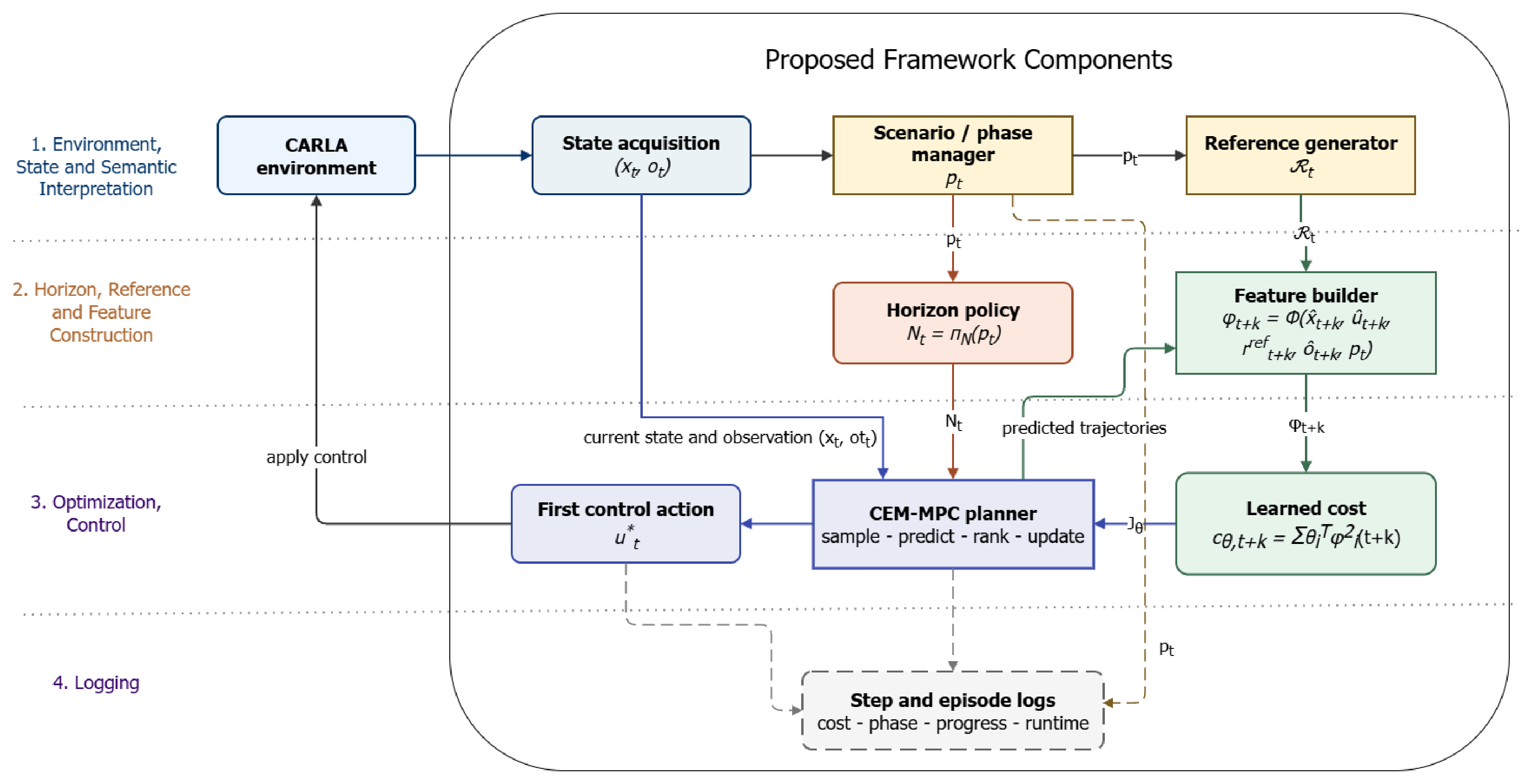
The implemented system follows a modular closed-loop architecture in which state acquisition, scenario interpretation, reference generation, feature construction, learned-cost evaluation, and control optimization are separated. This separation reflects the intended role of each component since scenario behavior is not encoded exclusively in the optimizer. Instead, the scenario manager determines the active driving context while the reference generator defines the desired vehicle path, represented as a target-lane centerline, a look-ahead waypoint, or a short reference trajectory. The learned cost model evaluates candidate behavior through a feature-weighted objective initialized from the learned-cost framework and augmented with lane-change-specific behavioral terms, while the CEM (Cross-Entropy Method) optimizer searches for the control sequence that minimizes the predicted cost over the selected horizon.

Figure 1 summarizes the information flow.

The closed-loop update can be summarized as

$$\begin{array}{cc}\hfill (x_t,o_t)& \to p_t\to {\mathcal{R}}_t\to N_t\hfill \\ & \to {\varphi }_{t:t+N_t}\to J_{\theta }\to u_t^{🟉}\to x_{t+1}.\hfill \end{array}$$

(21)

where $x_t$ represents the ego state, $o_t$ denotes obstacle or environmental information, $p_t$ is the recognized maneuver phase, ${\mathcal{R}}_t$ is the active reference representation, $N_t$ is the selected prediction horizon, $J_{\theta }$ is the MEDIRL-informed trajectory cost, and $u_t^{🟉}$ is the first control action applied to the simulated vehicle.

This modular architecture separates scenario interpretation, reference generation, learned-cost evaluation, and predictive optimization into distinct modules. The resulting decomposition allows maneuver semantics, reference definition, behavior evaluation, and control optimization to be modified independently while preserving the same closed-loop execution cycle.

4.2. Scenario Formulation and Maneuver Phases

The proof-of-concept is formulated around a lane-change task in which the ego vehicle must respond to an upcoming obstacle by transitioning from its current reference corridor to an admissible target corridor. The maneuver is defined through the constraints, reference objectives, and phase-transition conditions imposed on the ego vehicle, rather than through a fixed description of the road geometry.

The environment defines a feasible driving corridor $\mathcal{D}$, an obstacle-exclusion region $\mathcal{O}$, and a target reference set ${\mathcal{R}}^{\mathrm{tar}}$. The ego trajectory must satisfy the generic feasibility condition

$${\widehat{x}}_{t+k}\in \mathcal{D}\setminus \mathcal{O},k=1,\dots ,N_t,$$

(22)

while progressing toward the active reference supplied by the scenario manager. In this view, the lane-change scenario is a constrained reference-transition problem:

$${\mathcal{R}}^{\mathrm{cur}}⟶{\mathcal{R}}^{\mathrm{tar}},$$

(23)

where ${\mathcal{R}}^{\mathrm{cur}}$ denotes the current-lane reference and ${\mathcal{R}}^{\mathrm{tar}}$ denotes the target-lane reference.

The scenario manager maps the current state and environment into a maneuver phase:

$$p_t\in \mathcal{P}=\left\{p_{\mathrm{approach}},p_{\mathrm{transition}},p_{\mathrm{stabilization}}\right\}.$$

(24)

The exact transition thresholds are implementation specific, but the semantic meaning of each phase is general:

• $p_{\mathrm{approach}}$: the ego vehicle remains on the current reference while preparing for a required future transition;
• $p_{\mathrm{transition}}$: the ego vehicle actively moves from the current reference corridor toward the target reference corridor;
• $p_{\mathrm{stabilization}}$: the ego vehicle has reached the target corridor and must reduce residual lateral and heading error.

A strict success condition is defined as stable target-reference acquisition rather than momentary target-lane contact:

$$\begin{array}{cc}\hfill q_{\mathrm{success}}=& q_{\mathrm{target}}\wedge \left|e_y\right|\le {ϵ}_y\wedge \left|e_{\psi }\right|\le {ϵ}_{\psi }\hfill \\ \hfill & \wedge K_{\mathrm{stable}}\ge K_{\min }\wedge \neg q_{\mathrm{collision}}.\hfill \end{array}$$

(25)

Here, $q_{\mathrm{target}}$ indicates that the target reference region has been reached, $e_y$ is lateral tracking error, $e_{\psi }$ is heading error, $K_{\mathrm{stable}}$ counts consecutive stable steps, and $q_{\mathrm{collision}}$ indicates collision. This criterion is not a separate theoretical assumption; it is a measurable condition available within the implemented simulation framework.

4.3. Reference and Phase-Conditioned Horizon Policy

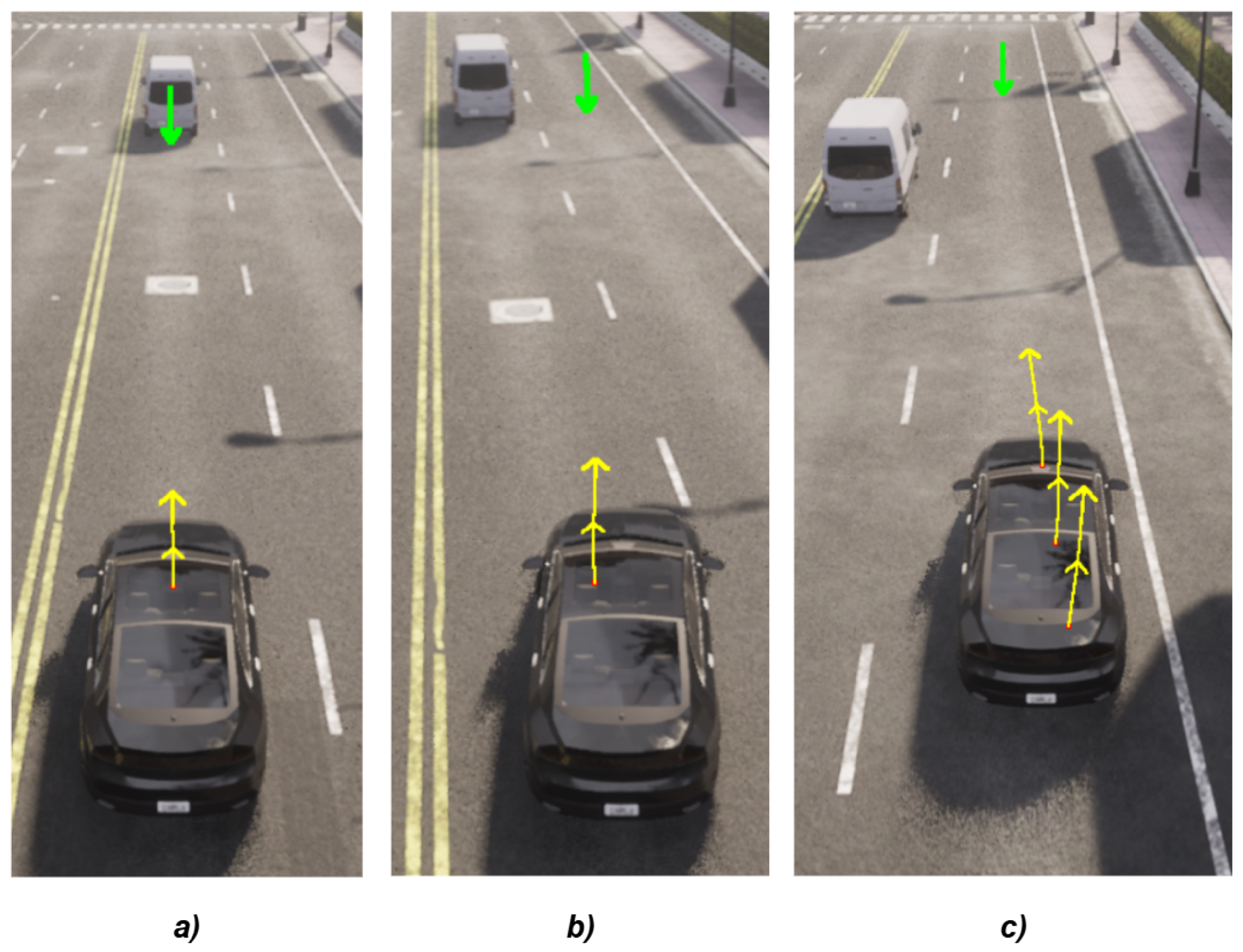
The reference generator provides the planner with the active reference context ${\mathcal{R}}_t$. During the approach phase, this reference remains associated with the current lane or preparation corridor. During the transition phase, the reference shifts toward the target corridor. During stabilization, the reference corresponds to target-lane keeping, as shown in Figure 2.

The prediction horizon follows the contextual formulation introduced in Equation (17). The present proof-of-concept evaluates the phase-only specialization

$$N_t={\pi }_N\left(p_t\right),$$

while $z_t$-conditioned adaptation is retained as a broader extension of the formulation. In the implemented rule-based version, the policy is phase-only:

$$N_t=\left\{\begin{array}{cc}{N}_{\mathrm{approach}},\hfill & p_t=p_{\mathrm{approach}},\hfill \\ N_{\mathrm{transition}},\hfill & p_t=p_{\mathrm{transition}},\hfill \\ N_{\mathrm{stabilization}},\hfill & p_t=p_{\mathrm{stabilization}}.\hfill \end{array}\right.$$

(26)

This policy is intentionally interpretable. It encodes the hypothesis that each phase imposes a different need for predictive depth:

• the approach phase requires sufficient foresight to anticipate the upcoming reference transition;
• the transition phase may benefit from additional predictive depth when evaluating lateral commitment, obstacle clearance, and target-lane progress;
• the stabilization phase is dominated increasingly by local reference convergence, making reduced predictive depth a plausible computationally efficient alternative.

The implemented comparison tests how this phase-conditioned allocation in Equation (26) compares with globally fixed horizons in terms of maneuver progress, tracking quality, smoothness, safety, and runtime.

4.4. Learned-Cost CEM–MPC Planner

The feature-based cost model and the CEM–MPC planner operate jointly: the cost model provides the objective used to score predicted trajectories, while the planner generates candidate trajectories whose quality is determined by that learned cost. The controller therefore does not optimize hand-designed tracking error alone; it evaluates sampled futures through a feature-based learned cost.

At each control step, the CEM planner samples candidate control sequences:

$$U_t^{\left(j\right)}\sim \mathcal{N}({\mu }_t,{\Sigma }_t),j=1,\dots ,M.$$

(27)

Each sequence is propagated through the prediction model, scored using $J_{\theta }^{\left(j\right)}\left(N_t\right)$, and ranked. The elite set is

$${\mathcal{E}}_t=\mathrm{Elite}\left({\left\{U_t^{\left(j\right)},J_{\theta }^{\left(j\right)}\right\}}_{j=1}^M\right),$$

(28)

and the sampling distribution is updated as

$${\mu }_t\leftarrow \mathrm{mean}\left({\mathcal{E}}_t\right),{\Sigma }_t\leftarrow \mathrm{cov}\left({\mathcal{E}}_t\right).$$

(29)

After the final CEM iteration, the first control action of the best sequence is applied:

$$u_t^{🟉}=U_{t,0}^{🟉}.$$

(30)

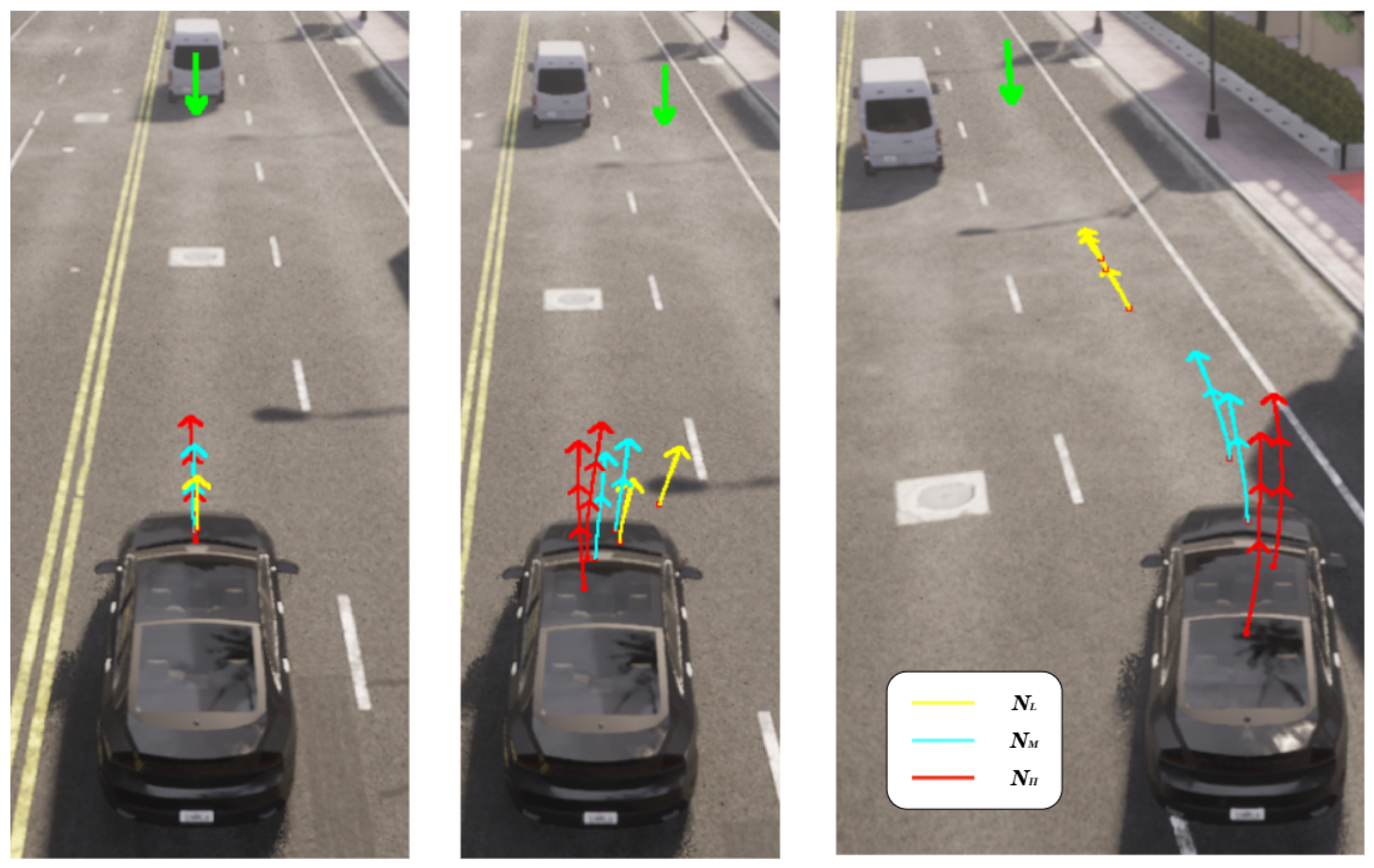
The dependence on $N_t$ enters at two levels. First, the number of predicted state transitions and feature evaluations changes with the selected horizon, translating into a corresponding prediction depth of every sampled candidate. Second, the effective evaluation of the fixed behavioral objective changes because different horizons expose the optimizer to different amounts of future progress, risk, and tracking error before the current action is selected. Therefore horizon properties not only influence computational runtime but also maneuver behaviour, as illustrated in Figure 3.

4.5. Experimental Protocol and Evaluated Hypothesis

The implemented experiment compares fixed-horizon and phase-aware horizon policies under the same learned cost, prediction model, scenario logic, and CEM optimization settings. The fixed-horizon policies defined in Equation (15) and the phase-aware policy defined in Equation (17) are evaluated under matched controller, scenario, and random-seed conditions. The phase-aware policy uses Equation (26), allowing the horizon to change when the recognized maneuver phase changes.

To ensure that the comparison isolates the effect of horizon selection, the experimental protocol keeps the following quantities fixed across policies:

• CARLA map and vehicle model,
• scenario geometry and trigger logic,
• learned cost weights $\theta$,
• CEM population size, elite count, and iteration count,
• simulation step size,
• control bounds,
• and random seeds or paired replay conditions where applicable

The logged quantities include:

• selected horizon $N_t$,
• maneuver phase $p_t$,
• cumulative and phase-wise learned cost,
• lateral and heading tracking errors,
• lane-change progress and target-lane acquisition,
• steering, steering variation, throttle, brake, and speed,
• obstacle gap and TTC-related risk,
• collision and success indicators,
• and per-step planner runtime.

Therefore, the experimental design supports three complementary levels of evidence: whole-episode comparison, phase-wise closed-loop analysis, and common-state counterfactual horizon comparison. Whole-episode metrics characterize realized maneuver outcomes; phase-wise metrics expose where those differences arise; and common-state replay isolates the direct effect of horizon length by evaluating alternative horizons from matched planner states. Together, these complementary perspectives support a structured evaluation of horizon-dependent behavior at both maneuver and planner-state levels.

The logged fixed-horizon experiments are first used to evaluate H1, defined in Section 3.7, by examining the relationship between horizon length and phase-specific planning performance. The implemented phase-aware policy is then compared with the corresponding fixed-horizon baselines to evaluate H2.

The following section presents the corresponding results, using maneuver success, collision occurrence, phase-wise and cumulative cost, lane-change progress, target-lane stabilization, tracking error, steering behavior, control smoothness, and planner runtime.

5. Analysis and Future Directions

This section presents the experimental results for the fixed-horizon and phase-aware policies. The comparison is first performed using whole-episode and phase-wise metrics, followed by common-state counterfactual analysis and controlled robustness evaluation. These complementary analyses are used to distinguish policy-level behavior, direct horizon sensitivity, and robustness to controlled scenario perturbations. The findings are then interpreted with respect to the hypotheses stated in Section 3.7 and positioned within the adaptive-horizon MPC literature in order to motivate future extensions of the proposed framework. Particular attention is given to distinguishing evidence for phase-dependent horizon requirements from evidence concerning the performance of any specific phase-aware horizon assignment.

5.1. Comparative Results

Three fixed-horizon baselines and the evaluated phase-aware horizon configurations are compared under the matched experimental conditions described in Section 4.5. The fixed-horizon experiments characterize the effect of prediction depth across the maneuver, while the phase-aware configurations evaluate whether this predictive depth can be allocated selectively according to maneuver phase. Among the evaluated phase-aware configurations, the 10–20–10 mapping represents the primary phase-conditioned policy considered in the final comparison, while the 20–40–10 mapping provides an additional reference for examining the effect of assigning greater predictive depth within the same phase structure.

The reported metrics characterize both overall maneuver performance and phase-specific behavior. Whole-episode metrics, reported in

Table 1. Whole-episode comparison of the evaluated horizon policies. Values are mean ± sample standard deviation.

Policy	${\mathit{J}}_{\mathbf{episode}}$	${\mathbf{RMSE}}_{\mathit{y}}$	${\mathbf{RMSE}}_{\mathit{\psi }}$	${\mathit{S}}_{\mathit{\delta }}$	Completion Time (s)	${\overline{\mathit{T}}}_{\mathbf{plan}}$ (ms)
Short fixed horizon ($H=10$)	$736.51\pm 41.82$	$0.995\pm 0.046$	$0.136\pm 0.004$	$60.24\pm 2.77$	$6.68\pm 0.18$	$32.58\pm 0.19$
Medium fixed horizon ($H=20$)	$1169.12\pm 142.67$	$1.122\pm 0.066$	$0.146\pm 0.006$	$89.47\pm 5.89$	$8.73\pm 0.71$	$66.45\pm 0.64$
Long fixed horizon ($H=40$)	$1702.14\pm 271.76$	$1.185\pm 0.143$	$0.162\pm 0.002$	$123.08\pm 2.56$	$11.50\pm 0.71$	$139.54\pm 7.19$
Phase-aware horizon (10–20–10)	$921.11\pm 50.81$	$1.050\pm 0.031$	$0.148\pm 0.002$	$65.48\pm 2.75$	$7.68\pm 0.44$	$27.21\pm 0.27$
Phase-aware horizon (20–40–10)	$1525.97\pm 130.59$	$1.131\pm 0.013$	$0.168\pm 0.009$	$89.93\pm 4.76$	$11.30\pm 0.99$	$74.59\pm 3.00$

, summarize complete maneuver execution, whereas phase-wise metrics isolate controller behavior within each maneuver phase.

$$J_{\mathrm{episode}}={\displaystyle \sum _{t=0}^T}{c}_{\theta }\left({\varphi }_t\right),$$

(31)

$${\mathrm{RMSE}}_y=\sqrt{{\displaystyle \frac{1}{T}}\sum _{t=0}^T{e}_y{\left(t\right)}^2},$$

(32)

$${\mathrm{RMSE}}_{\psi }=\sqrt{{\displaystyle \frac{1}{T}}\sum _{t=0}^T{e}_{\psi }{\left(t\right)}^2},$$

(33)

$$S_{\delta }={\displaystyle \sum _{t=1}^T}|{\delta }_t-{\delta }_{t-1}|.$$

(34)

and

$${\overline{T}}_{\mathrm{plan}}={\displaystyle \frac{1}{T}}{\displaystyle \sum _{t=0}^T}{T}_{\mathrm{plan}}\left(t\right).$$

(35)

Phase-wise metrics, as shown in

Table 2. Phase-wise closed-loop comparison of the evaluated horizon policies. The normalized phase cost is ${\overline{J}}_p=J_p/\left|{\mathcal{T}}_p\right|$. Values are mean ± sample standard deviation.

Policy	Phase	${\mathit{T}}_{\mathit{p}}$ (s)	${\mathit{J}}_{\mathit{p}}$	${\overline{\mathit{J}}}_{\mathit{p}}$	${\mathbf{RMSE}}_{\mathit{y},\mathit{p}}$	${\mathbf{RMSE}}_{\mathit{\psi },\mathit{p}}$	${\mathit{S}}_{\mathit{\delta },\mathit{p}}$	${\overline{\mathit{T}}}_{\mathbf{plan},\mathit{p}}$ (ms)
Short fixed horizon ($H=10$)	Approach	$2.50\pm 0.09$	$70.67\pm 3.02$	$1.413\pm 0.010$	$0.495\pm 0.012$	$0.007\pm 0.002$	$7.78\pm 1.02$	$32.60\pm 0.13$
	Transition	$4.18\pm 0.15$	$562.19\pm 49.57$	$6.728\pm 0.595$	$2.225\pm 0.108$	$0.297\pm 0.008$	$12.78\pm 1.04$	$40.41\pm 0.66$
	Stabilization	$15.00\pm 0.00$	$103.65\pm 18.71$	$0.345\pm 0.062$	$0.111\pm 0.020$	$0.047\pm 0.009$	$39.69\pm 1.84$	$30.47\pm 0.29$
Medium fixed horizon ($H=20$)	Approach	$2.66\pm 0.23$	$76.46\pm 8.14$	$1.434\pm 0.028$	$0.474\pm 0.020$	$0.009\pm 0.003$	$12.16\pm 1.65$	$65.37\pm 0.85$
	Transition	$6.06\pm 0.50$	$926.92\pm 137.26$	$7.618\pm 0.637$	$2.195\pm 0.086$	$0.280\pm 0.018$	$23.13\pm 2.96$	$80.60\pm 0.98$
	Stabilization	$15.00\pm 0.00$	$165.73\pm 0.73$	$0.552\pm 0.002$	$0.075\pm 0.012$	$0.046\pm 0.008$	$54.18\pm 2.34$	$61.29\pm 0.47$
Long fixed horizon ($H=40$)	Approach	$2.90\pm 0.07$	$85.20\pm 2.77$	$1.469\pm 0.012$	$0.456\pm 0.006$	$0.006\pm 0.000$	$12.81\pm 2.38$	$133.19\pm 4.88$
	Transition	$8.60\pm 0.78$	$1365.00\pm 298.56$	$7.890\pm 1.022$	$2.059\pm 0.189$	$0.279\pm 0.013$	$39.49\pm 1.45$	$163.50\pm 10.90$
	Stabilization	$15.00\pm 0.00$	$251.94\pm 24.02$	$0.840\pm 0.080$	$0.074\pm 0.005$	$0.043\pm 0.002$	$70.78\pm 1.63$	$126.96\pm 5.07$
Phase-aware horizon (10–20–10)	Approach	$2.55\pm 0.09$	$72.31\pm 2.63$	$1.418\pm 0.005$	$0.489\pm 0.010$	$0.007\pm 0.003$	$7.61\pm 1.06$	$23.03\pm 0.36$
	Transition	$5.13\pm 0.38$	$731.10\pm 58.43$	$7.120\pm 0.145$	$2.175\pm 0.037$	$0.300\pm 0.003$	$18.66\pm 0.33$	$55.49\pm 0.68$
	Stabilization	$15.00\pm 0.00$	$117.70\pm 40.81$	$0.392\pm 0.136$	$0.103\pm 0.016$	$0.046\pm 0.011$	$39.21\pm 3.89$	$16.31\pm 0.94$
Phase-aware horizon (20–40–10)	Approach	$2.68\pm 0.25$	$76.74\pm 8.83$	$1.433\pm 0.033$	$0.472\pm 0.021$	$0.009\pm 0.000$	$11.05\pm 0.55$	$65.73\pm 1.85$
	Transition	$8.63\pm 0.74$	$1286.45\pm 130.56$	$7.453\pm 0.115$	$1.947\pm 0.066$	$0.283\pm 0.009$	$37.16\pm 4.44$	$158.60\pm 3.08$
	Stabilization	$15.00\pm 0.00$	$162.79\pm 8.80$	$0.543\pm 0.029$	$0.163\pm 0.020$	$0.058\pm 0.001$	$41.71\pm 0.24$	$30.80\pm 0.45$

, decompose the same execution into approach, transition, and stabilization intervals. Let

$${\mathcal{T}}_p=\left\{t\mid p\left(t\right)=p\right\}$$

(36)

denote the set of closed-loop control steps assigned to phase p. The realized cumulative phase cost is defined as

$$J_p=\sum _{t\in {\mathcal{T}}_p}{c}_{{\theta }_p}\left({\varphi }_t\right),$$

(37)

where ${\theta }_p$ denotes the cost parameterization active during phase p.

Because the evaluated policies may spend different amounts of time in each phase, the duration-normalized phase cost is also reported:

$${\overline{J}}_p={\displaystyle \frac{J_p}{|{\mathcal{T}}_p|}}.$$

(38)

The phase-specific lateral and heading tracking errors are

$${\mathrm{RMSE}}_{y,p}=\sqrt{{\displaystyle \frac{1}{|{\mathcal{T}}_p|}}\sum _{t\in {\mathcal{T}}_p}{e}_y{\left(t\right)}^2},$$

(39)

and

$${\mathrm{RMSE}}_{\psi ,p}=\sqrt{{\displaystyle \frac{1}{|{\mathcal{T}}_p|}}\sum _{t\in {\mathcal{T}}_p}{e}_{\psi }{\left(t\right)}^2}.$$

(40)

Steering activity within phase p is measured through

$$S_{\delta ,p}=\sum _{\begin{array}{c}t\in {\mathcal{T}}_p\\ t>t_p^{\mathrm{start}}\end{array}}\left|{\delta }_t-{\delta }_{t-1}\right|,$$

(41)

while the mean planning time is

$${\overline{T}}_{\mathrm{plan},p}={\displaystyle \frac{1}{|{\mathcal{T}}_p|}}\sum _{t\in {\mathcal{T}}_p}{T}_{\mathrm{plan}}\left(t\right).$$

(42)

The purpose of the comparison is therefore not to establish that phase adaptation dominates every fixed horizon, but to determine whether predictive depth can be allocated according to maneuver phase while preserving successful and safe closed-loop execution and avoiding unnecessary computational expenditure.

The closed-loop results show that prediction horizon influences both maneuver behavior and computational demand, with effects that vary across maneuver phases.

The 10–20–10 policy preserves short prediction during approach and stabilization while increasing predictive depth during transition. In the matched comparison, it reaches the target reference without collision and improves target-entry lateral and heading error relative to fixed $H=10$.

These improvements do not imply uniform dominance over the fixed baseline, since later tracking and runtime metrics remain policy-dependent. The 20–40–10 configuration further shows that increasing predictive depth within the same phase structure does not automatically improve the overall trade-off.

The results therefore support phase-conditioned horizon allocation as a meaningful planning structure while leaving the specific phase horizons subject to further optimization.

The following common-state analysis isolates the direct effect of prediction horizon by re-evaluating alternative horizons from identical saved planner states.

5.2. Common-State Horizon Comparison

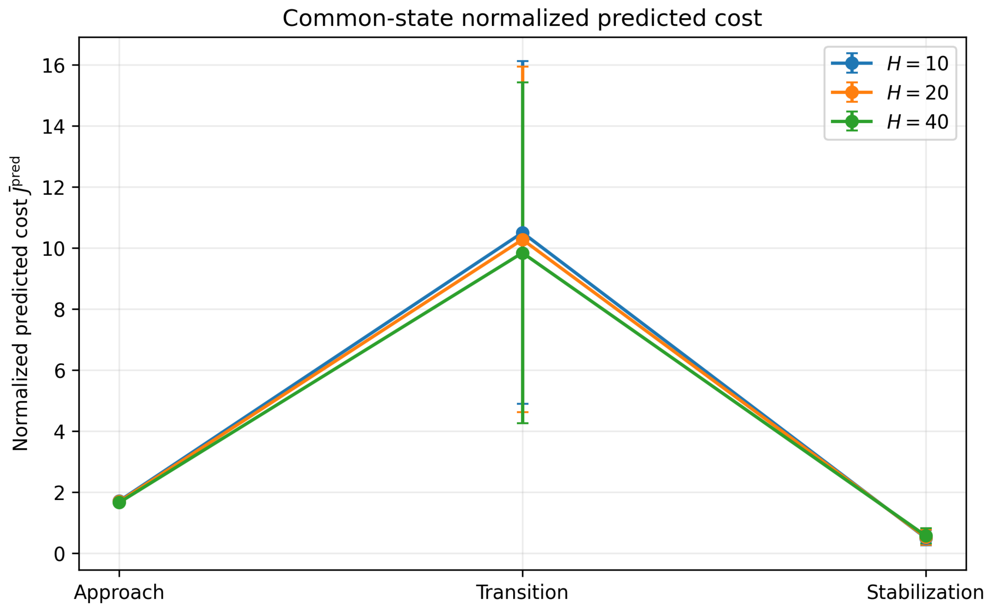
The closed-loop comparisons in Section 5.1 evaluate complete experiments produced under specific horizon policies. However, the resulting trajectories diverge since the ego vehicle reaches different states at corresponding moments of each experiment. Consequently, to expose the direct effect of prediction-horizon length, a supportive common-state comparison is performed. Planner snapshots are saved during the approach, transition, and stabilization phases of the closed-loop experiments. Starting from each saved state, the planner is re-evaluated offline using the candidate horizons

$$\mathcal{N}=\left\{10,20,40\right\}.$$

(43)

The vehicle state, scenario context, previous control input, cost parameterization, and CEM configuration are held fixed within each comparison. Only the candidate prediction horizon is varied. This comparison therefore isolates horizon-dependent planner behavior from differences caused by the preceding closed-loop trajectory. For candidate horizon N, the predicted horizon cost is normalized by the number of prediction steps:

$${\overline{J}}_N^{\mathrm{pred}}={\displaystyle \frac{J_N^{\mathrm{pred}}}{N}}.$$

(44)

This normalization is required because the unnormalized predicted cost accumulates over a different number of stages for each candidate horizon.

The terminal lateral and heading errors of the selected predicted trajectory are denoted by

$$\left|e_y^N\right|=\left|e_y(t+N)\right|,$$

(45)

and

$$\left|e_{\psi }^N\right|=\left|e_{\psi }(t+N)\right|.$$

(46)

Computational demand is represented by the runtime required to solve the planning problem $T_{\mathrm{plan}}^N$.

The aggregated common-state results are reported in

Table 3. Common-state counterfactual horizon comparison across maneuver phases. Each saved state is re-planned using the candidate horizons $H\in \{10,20,40\}$. Values report normalized predicted cost, terminal lateral error, and planning runtime as mean ± sample standard deviation.

Horizon	Metric	Approach	Transition	Stabilization
$H=10$	${\overline{J}}^{\mathrm{pred}}$	$1.712\pm 0.013$	$10.498\pm 5.611$	$0.501\pm 0.252$
	$|e_y^N|$ [m]	$0.0002\pm 0.0002$	$2.321\pm 1.322$	$0.123\pm 0.115$
	$T_{\mathrm{plan}}$ [ms]	$27.97\pm 1.31$	$34.23\pm 1.51$	$27.44\pm 1.48$
$H=20$	${\overline{J}}^{\mathrm{pred}}$	$1.691\pm 0.003$	$10.271\pm 5.657$	$0.523\pm 0.253$
	$|e_y^N|$ [m]	$0.0004\pm 0.0003$	$2.178\pm 1.345$	$0.119\pm 0.129$
	$T_{\mathrm{plan}}$ [ms]	$55.05\pm 1.11$	$69.64\pm 3.18$	$54.51\pm 2.60$
$H=40$	${\overline{J}}^{\mathrm{pred}}$	$1.659\pm 0.008$	$9.836\pm 5.589$	$0.572\pm 0.248$
	$|e_y^N|$ [m]	$0.0051\pm 0.0040$	$1.949\pm 1.295$	$0.140\pm 0.146$
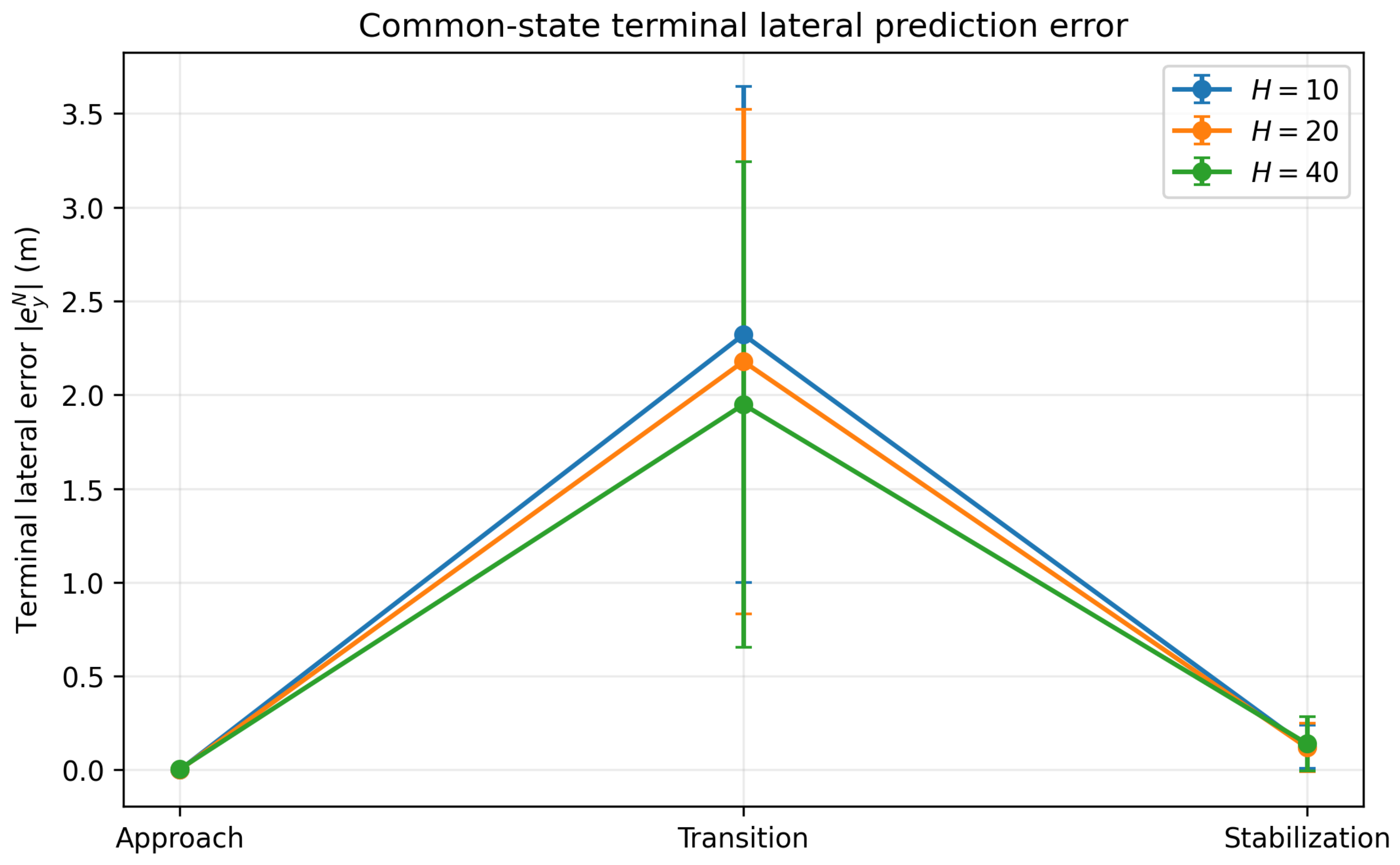
	$T_{\mathrm{plan}}$ [ms]	$111.23\pm 3.00$	$141.74\pm 5.96$	$109.30\pm 5.28$

, while the corresponding figures are Figure 4 and Figure 5. In contrast to the realized closed-loop costs $J_{\mathrm{episode}}$ and $J_p$, the quantities in this subsection describe predicted candidate trajectories generated from shared initial states. They are therefore used as diagnostic evidence for horizon sensitivity and are not combined directly with the realized closed-loop metrics.

The common-state comparison separates horizon-dependent planner behavior from differences caused by the preceding closed-loop trajectory. The normalized predicted cost, terminal-state quantities, and runtime jointly reveal that the effect of increasing the horizon is phase dependent. Longer horizons provide a larger prediction interval and may improve selected terminal quantities, but they also impose a substantial computational penalty. The empirical meaning of these trade-offs, together with the closed-loop results, is examined in Section 5.4. This comparison therefore provides direct support for H1: the relationship between predictive depth and planner performance is phase dependent. It does not by itself determine the preferred closed-loop horizon policy, since the predicted quantities must be interpreted together with the realized policy-level results.

5.3. Controlled Robustness Evaluation

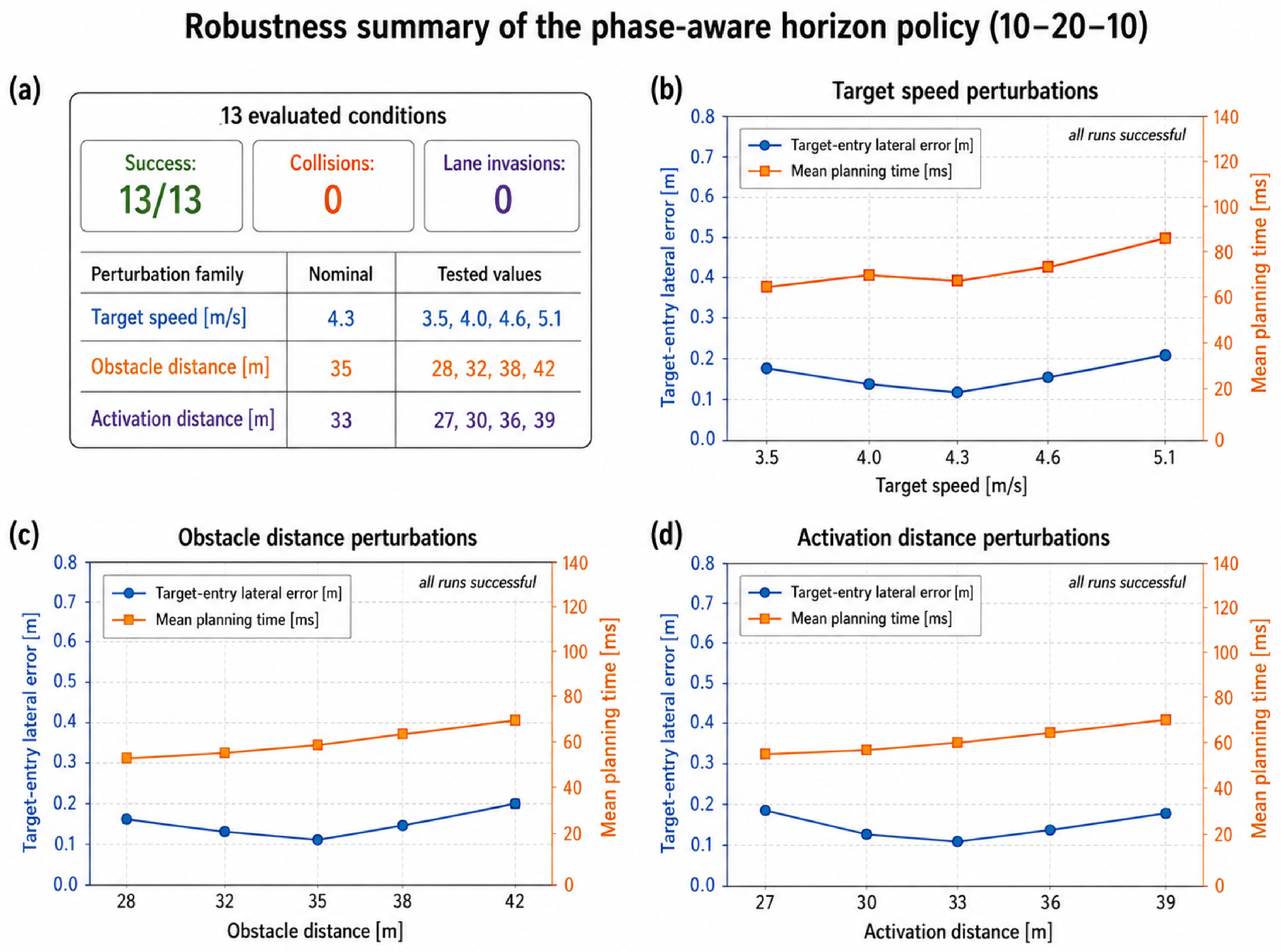
The phase-aware 10–20–10 policy is further evaluated under controlled perturbations of the nominal lane-change scenario. A one-factor-at-a-time protocol is used in which target speed, obstacle distance, and maneuver activation distance are varied independently while the horizon mapping, cost model, planner configuration, and CEM seed remain fixed.

The evaluated perturbation set is summarized in

Table 4. Controlled robustness conditions for the phase-aware 10–20–10 horizon policy.

Parameter	Nominal Value	Evaluated Values
Target speed [m/s]	$4.3$	$3.5,4.0,4.6,5.1$
Obstacle distance [m]	35	$28,32,38,42$
Activation distance [m]	33	$27,30,36,39$

.

Together with the nominal configuration, the study contains 13 evaluated conditions. Maneuver completion, collision occurrence, lane invasion, target-reference tracking, and planning runtime are recorded for each case.

Across the tested perturbation envelope, all 13 conditions satisfy the strict maneuver-success criterion, with no collision or lane invasion observed:

$$N_{\mathrm{success}}=N_{\mathrm{lane}\text{-}\mathrm{safe}}=13,N_{\mathrm{collision}}=N_{\mathrm{invasion}}=0.$$

(47)

These results show that the phase-aware policy remains feasible under the tested variations in vehicle speed and scenario geometry. The robustness evidence is interpreted within the tested perturbation envelope; the fixed CEM seed and one-factor-at-a-time design do not constitute multi-seed statistical validation.

The corresponding variation in tracking and computational behavior is shown in Figure 6. While these quantities vary across the tested conditions, successful and lane-safe maneuver execution is maintained throughout the evaluation.

5.4. Empirical Findings and Hypothesis Evaluation

The fixed-horizon, phase-wise, and common-state experiments support H1. Changing prediction depth alters both computational demand and planner behavior, while the magnitude and direction of these effects depend on the active maneuver phase. Additional prediction is most relevant during transition, whereas its benefit is less consistent during approach and stabilization and is accompanied by increased planning time.

Accordingly, a horizon that improves the predicted terminal state at a matched instant need not improve the realized closed-loop maneuver, because prediction depth also alters transition duration, accumulated cost, and control evolution.

The phase-aware experiments provide qualified support for H2. The selected policy preserves successful maneuver execution while allocating additional predictive depth during transition. The comparison with fixed horizons and alternative phase-aware allocation also indicates that the horizon values assigned within each phase remain consequential.

The controlled robustness evaluation complements these findings. Across the tested variations in target speed, obstacle distance, and activation distance, the phase-aware policy maintains successful and lane-safe maneuver execution. This supports its viability within the evaluated perturbation envelope, while broader statistical and scenario-level validation could be further examined.

Together, the experiments expose the following empirical findings:

• Prediction horizon influences both planner behavior and computational demand.
• The effect of prediction depth depends on the active maneuver phase.
• Greater predictive depth does not automatically improve realized closed-loop performance.
• Phase conditioning provides an interpretable structure for allocating predictive effort, while the specific horizon assigned to each phase remains a design variable.
• Whole-episode, phase-wise, common-state, and robustness evidence provide complementary views of horizon-policy behavior.

5.5. Positioning of the Empirical Findings

Existing adaptive-horizon MPC methods commonly select prediction depth from vehicle speed, path curvature, tracking error, stability indicators, environmental complexity, or learned policies. The present study instead focuses specifically on maneuver phase as an explicit and interpretable scheduling signal within a learned-cost CEM-MPC framework.

This positioning also places the phase-aware adaptation at a higher level of the planning context: horizon selection is conditioned first on the recognized maneuver phase, rather than reacting directly to isolated vehicle- or road-level variables.

The empirical results indicate that horizon adaptation should not be interpreted only as a computational adjustment. Prediction depth also changes how the planner evaluates future progress, tracking error, and risk throughout maneuver execution. At the same time, the experiments show that increasing horizon length does not automatically improve closed-loop behavior, reinforcing the importance of conditioning predictive effort on the current maneuver context.

The contribution is therefore not a claim of a universally optimal phase-dependent horizon assignment, but evidence that maneuver phase provides a meaningful and interpretable context for horizon selection in the evaluated lane-change scenario.

5.6. Contribution and Future Directions

The analysis supports three connected contributions. First, it provides a phase-conditioned formulation of prediction-horizon selection for a lane-change maneuver. Second, it integrates this formulation with a learned-cost CEM-MPC architecture in which the selected phase changes the predictive depth of sampled candidate controls. Third, it establishes a phase-wise evaluation methodology that explains when and why different horizons affect maneuver progress, tracking behavior, control evolution, and runtime.

The findings also orient the next development stages of the framework. The present rule-based policy can be expanded from

$$N_t={\pi }_N\left(p_t\right)$$

(48)

toward the broader contextual policy already introduced in Equation (17):

$$N_t={\pi }_N(p_t,z_t),$$

(49)

where $z_t$ may include speed, tracking error, obstacle gap, maneuver progress, risk, and computational state. In this extension, the recognized maneuver phase can act as a prior scheduling context, while $z_t$ provides finer adaptation within the active phase. Conceptually, this can be expressed as

$$p_t⟶{\pi }_N^{\left(p_t\right)}⟶z_t⟶N_t.$$

(50)

preserving maneuver phase as the principal interpretable structure while allowing context-sensitive refinement within each phase. A second direction is to study joint predictive configuration. The current work adapts the horizon while keeping the phase-conditioned cost and reference configuration, prediction model, and CEM settings fixed. The phase-dependent findings suggest a broader hierarchical architecture in which maneuver state may condition not only the reference and horizon, but also the active feature representation, learned cost model, sampling population, elite ratio, or temporal discretization:

$$p_t⟶\left\{{\mathcal{R}}_t,N_t,{\varphi }_t,{\theta }_t,{\Omega }_{\mathrm{CEM},t}\right\}.$$

(51)

A third direction is broader validation. The current proof-of-concept should be extended to additional CARLA maps, different vehicle speeds, dynamic obstacles, alternative lane-change geometries, and further maneuvers such as merging, overtaking, intersection negotiation, and recovery. Such experiments could further examine whether the phase-dependent relationships observed here persist across scenario families and whether the same scheduling structure can transfer between maneuvers.

Finally, the phase-aware evaluation itself should be retained as the framework expands. The present results indicate that aggregate episode metrics may obscure local advantages and failures. Future learned or optimization-based horizon policies should therefore continue to be analyzed through both whole-episode outcomes and phase-resolved behavioral evidence, complemented where appropriate by common-state and robustness analysis.

6. Conclusions

This paper investigates the role of prediction horizon selection in learned-cost receding-horizon planning for autonomous driving and presents a phase-aware horizon policy that adapts predictive foresight according to the requirements of different driving maneuvers. Rather than treating the prediction horizon as a globally fixed optimization parameter, the proposed framework allocates planning foresight according to the operational demands of each maneuver while preserving a unified planning architecture.

The experimental evaluation demonstrated that prediction horizon substantially influences both computational effort and closed-loop driving behavior. While fixed horizons exhibited distinct advantages during different stages of the lane-change maneuver, the proposed phase-aware policy showed that predictive depth can be allocated selectively across maneuver phases while preserving successful maneuver execution and avoiding uniformly large horizons. The common-state evaluation further isolated the influence of horizon selection by comparing alternative planning decisions from identical driving states, providing a clearer interpretation of the relationship between prediction depth, planning performance, and computational cost. Controlled perturbation experiments further indicated that the phase-conditioned policy remained successful and lane-safe across the evaluated variations in speed and scenario geometry.

Although the present implementation employs a predefined phase-conditioned horizon policy, the proposed framework establishes a modular foundation for future data-driven horizon adaptation strategies. More broadly, the findings suggest that prediction horizon should be regarded as a behavioral planning parameter rather than solely as an optimization setting and that maneuver phase can provide an explicit and interpretable context for allocating predictive effort, opening a direction toward hierarchical semantic and context-aware horizon adaptation in autonomous driving.