Zero-Sum Game-Based Practical Predefined-Time Reinforcement Learning for Robust Tracking Control of Highly Flexible Aircraft

Abstract

This paper develops a zero-sum game-based practical predefined-time reinforcement learning method for robust tracking control of highly flexible aircraft. First, the disturbed tracking problem of highly flexible aircraft is transformed into a min–max optimal control problem, where the controller minimizes the infinite-horizon performance index and the adversarial disturbance maximizes it. Then, a critic neural network is used to approximate the solution of the Hamilton–Jacobi–Isaacs equation online, and a fractional-power critic-update law is constructed so that the critic weight estimation error converges to a bounded neighborhood within a user-predefined time. The boundedness of closed-loop and practical predefined-time convergence of critic weight estimation error are rigorously proven. Several simulations are conducted to verify the advancement, effectiveness and robustness of this control algorithm. Overall, the results demonstrate that the proposed method provides an effective practical predefined-time learning framework for robust tracking control of highly flexible aircraft.

1. Introduction

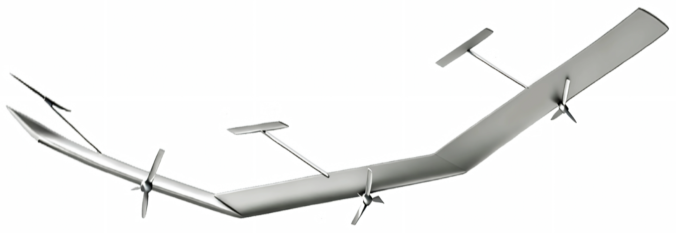
Highly flexible aircraft (HFA) serve as a representative benchmark for advanced flight control due to their lightweight high-aspect-ratio wings and strong aeroelastic coupling. Nonlinear aeroelasticity and flight dynamics must be treated together for HFA, since flexible deformation changes both the structural response and rigid-body motion [1]. Large elastic deformation in flight induces strong rigid–flexible coupling in HFA, resulting in pronounced nonlinearities and modeling uncertainties. These characteristics make controller design for HFA particularly challenging [2].

A variety of nonlinear control methods have been developed for highly flexible aircraft. Gregory used modified nonlinear dynamic inversion to improve flexible-aircraft control, but this type of approach still relies on a carefully constructed dynamic model [3]. Patil and Hodges studied output-feedback control for nonlinear aeroelastic response, showing that feedback design can suppress flexible response when the aeroelastic model is available [4]. Shearer and Cesnik proposed a trajectory-control architecture for very flexible aircraft, and Raghavan and Patil extended trajectory control ideas to high-aspect-ratio flying wings [5,6]. Gust and load-alleviation studies then introduced robust control, model-predictive control, and LQG-based designs to improve performance under atmospheric excitation [7]. Cook et al. emphasized robust gust alleviation and stabilization for highly flexible aircraft, while Haghighat et al. used model-predictive control for gust-load alleviation [8,9]. Liu et al. showed that LQG-based model-predictive control can be effective for gust-load alleviation in flexible aircraft [10]. However, Qu and Annaswamy pointed out that trim drift, unmeasured flexible modes, and actuator anomalies can exceed the robustness margin of conventional linear output-feedback designs, motivating adaptive output-feedback control with closed-loop reference models [11].

Reinforcement learning (RL) and approximate dynamic programming (ADP) provide another route because they learn value functions and policies from system data rather than requiring a completely known drift model. Lewis and Vrabie connected reinforcement learning and ADP to feedback control, and Lewis et al. later summarized how natural decision methods can be used to design optimal adaptive controllers [12,13]. Kiumarsi et al. reviewed optimal and autonomous control using reinforcement learning, showing the breadth of ADP/RL in modern feedback-control design [14]. For continuous-time systems, Vrabie et al. introduced policy-iteration-based adaptive optimal control, and Jiang and Jiang developed computational adaptive optimal control for systems with completely unknown dynamics [15,16]. Zhu et al. further showed that integral reinforcement learning can be used for suboptimal output-feedback control of partially unknown linear continuous-time systems [17]. Then, Peng and Ma used online integral RL to stabilize an uncertain HFA using full-state and output-feedback information, reducing the dependence on exact drift dynamics [2]. Nevertheless, RL controllers for HFA still face two important difficulties: the learning convergence time is not explicitly assigned by the designer, and external disturbances are not always treated as worst-case strategic inputs during the learning process.

Zero-sum differential games provide a natural framework for robust RL because the controller minimizes the performance index while the disturbance attempts to maximize it. Abu-Khalaf et al. used neurodynamic programming and zero-sum games to handle constrained control, which established an important link between Hamiltonian function equations and robust learning-based control [18]. An efficient adaptive synchronization criteria was developed in [19] for fractional-order fuzzy neural networks with uncertain parameters, providing a useful perspective on adaptive control of uncertain nonlinear systems. Vamvoudakis and Lewis then developed an online solution for nonlinear two-player zero-sum games using synchronous policy iteration [20]. More recently, Wang et al. combined safe reinforcement learning, fixed-time stability, and zero-sum games to address nonlinear systems with external disturbances and obstacle-avoidance awareness [21]. A novel ESO-enhanced actor–critic RL method for robust marine-vessel tracking was developed in [22]. However, fixed-time bounds can still be conservative, and the designer may not be able to set the actual convergence time directly as a mission parameter.

To directly set the convergence time, Yuan et al. developed neural adaptive fixed-time control for nonlinear systems with full-state constraints, illustrating the value of neural approximation in time-constrained control [23]. An efficient fixed-time event-triggered control was proposed for distributed underwater vehicles in [24]. Wang, Cao, and Liu then proposed adaptive fuzzy control with both predefined time and predefined accuracy, emphasizing that convergence time and convergence accuracy can be assigned in advance for engineering systems [25]. A new standard was developed in [26] to measure the lowest convergence rate for leader–follower consensus under communication delays. Efficient cooperative consensus tracking control was investigated in [27] for multi-agent systems on cooperation–competition networks with asynchronous information exchange. Ni and Shi developed predefined-time adaptive neural control with output constraints, and Liu et al. studied predefined-time backstepping for strict-feedback nonlinear systems [28,29]. Related predefined-time stability results further support the use of user-specified time parameters in nonlinear systems [30]. However, a zero-sum game-based predefined-time reinforcement learning method has not been designed for highly flexible aircraft.

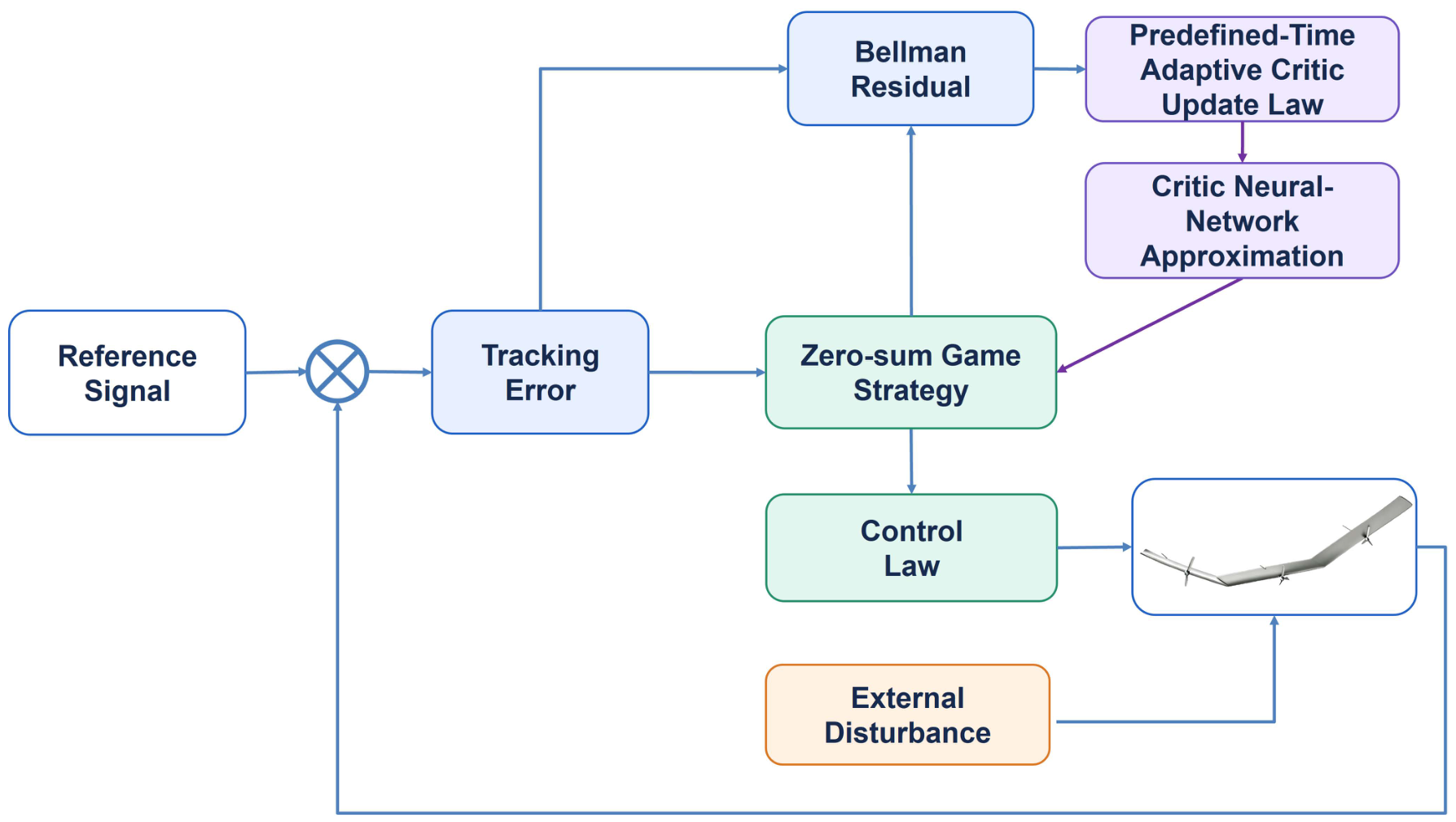
Motivated by the above discussions, this work develops a zero-sum game-based practical predefined-time reinforcement learning method for robust tracking control of highly flexible aircraft. The main contributions are summarized as follows:

(1) Compared with existing RL-based control methods for highly flexible aircraft [2], where external disturbances are treated as exogenous signals, a zero-sum differential-game architecture is constructed to explicitly characterize the worst-case interaction between the controller and disturbance, thereby converting the robust tracking problem into a min–max optimal control problem.

(2) Compared with conventional zero-sum ADP/RL methods [18,20] and the recent fixed-time zero-sum RL method [21], the critic weight-estimation error is guaranteed to converge to a bounded neighborhood within the predefined time.

(3) In contrast with predefined-time adaptive neural/fuzzy and backstepping control methods [25,28,29], the proposed predefined-time mechanism is incorporated into the critic learning process of the zero-sum game. The practical predefined-time convergence of the critic weight-estimation error and uniform ultimate boundedness of the overall closed-loop tracking system are rigorously established.

2. Problem Statement

2.1. Preliminaries

Consider the following autonomous nonlinear system:

$$\dot{\mathit{x}}\left(t\right)=\mathit{f}\left(\mathit{x}\left(t\right)\right),\mathit{x}\left(0\right)={\mathit{x}}_0,t\ge 0,$$

(1)

where $\mathit{x}\left(t\right)\in {\mathbb{R}}^n$ is the state vector, ${\mathit{x}}_0$ is the initial state, t is the time, and the nonlinear function expressed as $\mathit{f}:{\mathbb{R}}^n\to {\mathbb{R}}^n$ is continuous and satisfies $\mathit{f}\left(\mathbf{0}\right)=\mathbf{0}$.

Definition 1.

Let $T\left({\mathit{x}}_0\right)$ be the physical time required for the state starting from ${\mathit{x}}_0$ to reach the origin. If ${sup}_{{\mathit{x}}_0\in {\mathbb{R}}^n}T\left({\mathit{x}}_0\right)\le T_c$ holds with a given time constant ($T_c>0$), then the origin is globally predefined-time stable.

Lemma 1.

For the above nonlinear system, suppose that there exists a continuously differentiable, positive-definite, and radially unbounded Lyapunov function ($V:{\mathbb{R}}^n\to {\mathbb{R}}_{\ge 0}$), and suppose that for a given time constant ($T_c>0$) and a parameter ($\eta \in (0,1)$), the derivative of V along the system trajectory satisfies [25]

$$\dot{V}\le -{\displaystyle \frac{\pi }{\eta T_c}}\left(V{\left(\mathit{x}\left(t\right)\right)}^{1-\eta /2}+V{\left(\mathit{x}\left(t\right)\right)}^{1+\eta /2}\right)+b.$$

(2)

Then, the origin is globally practical predefined-time, the convergence-time upper bound is determined by the physical constant ($2T_c$), and V converges to the region expressed as $V\le {\displaystyle \frac{\eta b{T}_c}{\pi }}$.

Lemma 2.

For any real sequence (${\left\{y_j\right\}}_{j=1}^m\in \mathbb{R}$) and any $\eta \in (0,1)$, the following inequalities hold [23]:

$${\left({\displaystyle \sum _{j=1}^m}{y}_j^2\right)}^{{\displaystyle \frac{2-\eta }{2}}}\le {\displaystyle \sum _{j=1}^m}{\left|y_j\right|}^{2-\eta },$$

(3)

$$m^{-\eta /2}{\left({\displaystyle \sum _{j=1}^m}{y}_j^2\right)}^{{\displaystyle \frac{2+\eta }{2}}}\le {\displaystyle \sum _{j=1}^m}{\left|y_j\right|}^{2+\eta }.$$

(4)

2.2. Dynamics of Highly Flexible Aircraft

The aircraft under consideration is shown in Figure 1 [31]. It comprises three identical rigid wing bodies connected through hinges. Each rigid panel includes a propeller for thrust production, an aileron along the aft of the main wing, and an elevator attached at the end of the boom. In comparison with conventional flexible aerial vehicles, elastic modal behaviors exhibited by HFA are simplified and represented by dihedral angle parameters [31]. The dynamic modeling methodology adopted for HFA aligns fully with that utilized for standard rigid-body aircraft platforms. Concentrated substantial structural deflection occurs at the hinge interface between dual wing panels, rendering the model capable of reproducing flexible structural deformation responses.

The longitudinal control-oriented nonlinear model is written as [32]

$$\left\{\begin{array}{cc}\hfill \dot{V}& ={\displaystyle \frac{T\cos \alpha -D}{m}}-g\sin \gamma ,\hfill \\ \hfill \dot{\alpha }& =-{\displaystyle \frac{T\sin \alpha +L}{mV}}+q+{\displaystyle \frac{g\cos \gamma }{V}},\hfill \\ \hfill \dot{h}& =V\sin \gamma ,\hfill \\ \hfill \dot{\theta }& =q,\hfill \\ \hfill \dot{q}& ={\displaystyle \frac{M-2c_2\sin \left(\eta \right)\cos \left(\eta \right)\dot{\eta }q}{c_1+c_2{\sin }^2\left(\eta \right)}},\hfill \\ \hfill \ddot{\eta }& ={\displaystyle \frac{H-{\kappa }_c\dot{\eta }-{\kappa }_k\eta +d_1-d_2}{d_3}},\hfill \end{array}\right.$$

(5)

where V is velocity, $\gamma =\theta -\alpha$ is the flight-path angle, h is the altitude, $\alpha$ is the angle of attack, $\theta$ is the pitch angle, q is the pitch rate, $\eta$ is the dihedral angle describing the elastic model, T is total thrust, D is drag, L is lift, and M and H are the total moment and angular moment related to control inputs. The coefficients are

$$\begin{array}{cc}\hfill c_1& =3I_{yy}^{\ast },c_2=2I_{zz}^{\ast }-2I_{yy}^{\ast }+{\displaystyle \frac{m^{\ast }{s}^2}{6}},\hfill \\ \hfill d_1& ={\displaystyle \frac{s}{2}}{m}^{\ast }\left[(\dot{V}\sin \alpha +V\cos \alpha \dot{\alpha })\cos \eta -V\sin \alpha \sin \eta \dot{\eta }-{\displaystyle \frac{2s}{3}}\cos \eta \sin \eta {\dot{\eta }}^2\right],\hfill \\ \hfill d_2& =\left(I_{yy}^{\ast }-I_{zz}^{\ast }-{\displaystyle \frac{m^{\ast }{s}^2}{12}}\right)\sin \eta \cos \eta q^2-{\displaystyle \frac{m^{\ast }s}{2}}\cos \eta V\cos \alpha q,\hfill \\ \hfill d_3& =I_{x_3{x}_3}^{\ast }+m^{\ast }\left({\displaystyle \frac{s^2}{4}}+{\displaystyle \frac{s^2}{6}}{\cos }^2\eta \right).\hfill \end{array}$$

(6)

The compact nonlinear HFA model is

$$\dot{\mathit{X}}=\mathit{f}(\mathit{X},\mathit{U}),\mathit{X}={[V,\alpha ,h,\theta ,q,\eta ,\dot{\eta }]}^{\mathrm{T}},$$

(7)

with the five-input vector expressed as

$$\mathit{U}={[{\delta }_t,{\delta }_{a,c},{\delta }_{a,o},{\delta }_{e,c},{\delta }_{e,o}]}^{\mathrm{T}}.$$

(8)

After linearization around a trim point $({\mathit{X}}_0,{\mathit{U}}_0)$ satisfying $\mathit{f}({\mathit{X}}_0,{\mathit{U}}_0)=\mathbf{0}$, the local model is

$$\dot{\mathit{x}}=\mathit{A}\mathit{x}+\mathit{B}\mathit{u},$$

(9)

where $\mathit{x}=\mathit{X}-{\mathit{X}}_0$ and $\mathit{u}=\mathit{U}-{\mathit{U}}_0$. In the simulation of this paper, the altitude deviation is not controlled explicitly, and the six-state vector is

$$\mathit{x}\left(t\right)={\left[V\right(t),\alpha (t),\theta (t),q(t),\eta (t),\dot{\eta }(t\left)\right]}^{\mathrm{T}}\in {\mathbb{R}}^6,$$

(10)

with the five-input vector ($\mathit{u}\left(t\right)\in {\mathbb{R}}^5$) inherited from $\mathit{U}$.

2.3. Disturbed Tracking-Error Dynamics

Consider the following linear system subject to unknown external disturbance:

$$\dot{\mathit{x}}\left(t\right)=\mathit{A}\mathit{x}\left(t\right)+\mathit{B}\mathit{u}\left(t\right)+\mathit{d}\left(t\right),$$

(11)

where $\mathit{u}\left(t\right)\in {\mathbb{R}}^5$ is the control input vector, $\mathit{d}\left(t\right)\in {\mathbb{R}}^6$ is the unknown external bounded disturbance, $\mathit{A}\in {\mathbb{R}}^{n\times n}$ is the system matrix, and $\mathit{B}\in {\mathbb{R}}^{n\times m}$ is the input coupling matrix.

The error dynamics model is

$$\dot{\mathit{z}}\left(t\right)=\mathit{F}\left(t\right)+\mathit{B}\mathit{u}\left(t\right)+\mathit{d}\left(t\right),$$

(12)

where

$$\mathit{z}\left(t\right)=\mathit{x}\left(t\right)-{\mathit{x}}_d\left(t\right),\mathit{F}\left(t\right)=\mathit{A}\mathit{x}\left(t\right)-{\dot{\mathit{x}}}_d\left(t\right),$$

(13)

${\mathit{x}}_d\left(t\right)$ is the the desired reference signal, and ${\dot{\mathit{x}}}_d\left(t\right)$ denotes the derivative of the reference signal. In this paper, $\parallel ·\parallel$ denotes the vector 2-norm or the induced matrix 2-norm.

The control objective is to design an RL algorithm and a parameter-update strategy such that: (i) the neural-network parameter estimation error vector ($\tilde{\mathit{W}}\left(t\right)$) converges to a bounded neighborhood within the strict predefined time ($T_w$) and (ii) under the worst external disturbance $\mathit{d}\left(\mathit{z}\right(t\left)\right)$, the tracking error can achieve bounded convergence.

3. Zero-Sum Game-Based Practical Predefined-Time RL Controller Design

3.1. Zero-Sum-Game Optimal Control

For the error system (12), we define the nonlinear utility function ($\mathcal{J}:{\mathbb{R}}^n\times {\mathbb{R}}^m\times {\mathbb{R}}^n\to \mathbb{R}$) to evaluate the dynamic-system performance:

$$\mathcal{J}(\mathit{z}\left(t\right),\mathit{u}\left(t\right),\mathit{d}\left(t\right))={\mathit{z}}^{\mathrm{T}}\left(t\right)\mathit{Q}\mathit{z}\left(t\right)+{\mathit{u}}^{\mathrm{T}}\left(t\right)\mathit{R}\mathit{u}\left(t\right)-{\delta }^2{\mathit{d}}^{\mathrm{T}}\left(t\right)\mathit{d}\left(t\right),$$

(14)

where $\mathit{Q}\in {\mathbb{R}}^{n\times n}$ is the tracking-error weight, $\mathit{R}\in {\mathbb{R}}^{m\times m}$ is the control-input weight, and $\delta >0$ is the disturbance weight.

The optimal value function ($V_c\left(t\right)$) is defined as the min–max functional of the utility index over the infinite horizon:

$$V_c\left(t\right)=\underset{\mathit{u}}{min}\underset{\mathit{d}}{max}{\int }_0^{\infty }\mathcal{J}(\mathit{z}\left(t\right),\mathit{u}\left(t\right),\mathit{d}\left(t\right))\mathrm{d}t.$$

(15)

For $V_c\left(t\right)$, the differential-game Hamiltonian ($H(\mathit{z}\left(t\right),\nabla V_c\left(\mathit{z}\left(t\right)\right),\mathit{u}\left(t\right),\mathit{d}\left(t\right))$) is constructed as

$$\begin{array}{cc}\hfill H=& {\mathit{z}}^{\mathrm{T}}\left(t\right)\mathit{Q}\mathit{z}\left(t\right)+{\mathit{u}}^{\mathrm{T}}\left(t\right)\mathit{R}\mathit{u}\left(t\right)-{\delta }^2{\mathit{d}}^{\mathrm{T}}\left(t\right)\mathit{d}\left(t\right)\hfill \\ & +\nabla V_c^{\mathrm{T}}\left(\mathit{z}\left(t\right)\right)\left(\mathit{F}\left(t\right)+\mathit{B}\mathit{u}\left(t\right)+\mathit{d}\left(t\right)\right).\hfill \end{array}$$

(16)

Taking the extremum derivatives with respect to the control and disturbance variables gives

$${\displaystyle \frac{\partial H}{\partial \mathit{u}\left(t\right)}}=2\mathit{R}\mathit{u}\left(t\right)+{\mathit{B}}^{\mathrm{T}}\nabla V_c\left(t\right)=\mathbf{0},$$

(17)

$${\displaystyle \frac{\partial H}{\partial \mathit{d}\left(t\right)}}=-2{\delta }^2\mathit{d}\left(t\right)+\nabla V_c\left(\mathit{z}\left(t\right)\right)=\mathbf{0}.$$

(18)

Therefore, the optimal feedback Nash strategies are

$${\mathit{u}}^{\ast }\left(t\right)=-{\displaystyle \frac{1}{2}}{\mathit{R}}^{-1}{\mathit{B}}^{\mathrm{T}}\nabla V_c^{\ast }\left(t\right),{\mathit{d}}^{\ast }\left(t\right)={\displaystyle \frac{1}{2{\delta }^2}}\nabla V_c^{\ast }\left(t\right).$$

(19)

According to the extremum conditions, the optimal feedback strategies satisfy the steady-state HJI partial differential equation, i.e.,

$$H(\mathit{z}\left(t\right),\nabla V_c\left(t\right),{\mathit{u}}^{\ast }\left(\mathit{z}\left(t\right)\right),{\mathit{d}}^{\ast }\left(\mathit{z}\left(t\right)\right))=0.$$

(20)

3.2. Critic Neural-Network Approximation

A critic neural network is adopted to parameterize and reconstruct the optimal value function ($V_c\left(\mathit{z}\left(t\right)\right)$):

$$V_c\left(\mathit{z}\left(t\right)\right)={\mathit{W}}^{\ast \mathrm{T}}\mathit{\psi }\left(\mathit{z}\left(t\right)\right)+\epsilon \left(\mathit{z}\left(t\right)\right).$$

(21)

Taking the gradient with respect to the state variable yields

$$\nabla V_c\left(\mathit{z}\left(t\right)\right)=\nabla {\mathit{\psi }}^T\left(\mathit{z}\left(t\right)\right){\mathit{W}}^{\ast }+\nabla \epsilon \left(\mathit{z}\left(t\right)\right).$$

(22)

Here, ${\mathit{W}}^{\ast }\in {\mathbb{R}}^M$ is the ideal network weight vector, M is the number of hidden nodes, and $\mathit{\psi }:{\mathbb{R}}^n\to {\mathbb{R}}^M$ is the activation basis vector. The approximation residual satisfies

$$\parallel \epsilon \left(\mathit{z}\left(t\right)\right)\parallel \le {\epsilon }_c,\parallel \nabla \epsilon \left(\mathit{z}\left(t\right)\right)\parallel \le {\epsilon }_{dc}.$$

(23)

Here, ${\epsilon }_c>0$ and ${\epsilon }_{dc}>0$ denote the upper bounds of the approximation residual ($\epsilon \left(z\right(t\left)\right)$) and its gradient ($\nabla \epsilon \left(z\right(t\left)\right)$), respectively. Thus, the optimal control and disturbance strategies can be written as

$${\mathit{u}}^{\ast }\left(t\right)=-{\displaystyle \frac{1}{2}}{\mathit{R}}^{-1}{\mathit{B}}^{\mathrm{T}}\left(\nabla {\mathit{\psi }}^T\left(\mathit{z}\left(t\right)\right){\mathit{W}}^{\ast }+\nabla \epsilon \left(\mathit{z}\left(t\right)\right)\right),$$

(24)

$${\mathit{d}}^{\ast }\left(t\right)={\displaystyle \frac{1}{2{\delta }^2}}\left(\nabla {\mathit{\psi }}^T\left(\mathit{z}\left(t\right)\right){\mathit{W}}^{\ast }+\nabla \epsilon \left(\mathit{z}\left(t\right)\right)\right).$$

(25)

The critic neural network approximates the optimal value function as

$${\widehat{V}}_c(\mathit{z},t)={\widehat{\mathit{W}}}^{\mathrm{T}}\left(t\right)\mathit{\psi }\left(\mathit{z}\right),$$

(26)

whose state gradient is directly obtained as

$$\nabla {\widehat{V}}_c(\mathit{z},t)=\nabla {\mathit{\psi }}^{\mathrm{T}}\left(\mathit{z}\right)\widehat{\mathit{W}}\left(t\right).$$

(27)

Substituting this learned value-function gradient into the analytical saddle-point mappings yields the implementable control policy:

$$\begin{array}{cc}\hfill {\widehat{\mathit{u}}}_c\left(\mathit{z}\left(t\right)\right)& =-{\displaystyle \frac{1}{2}}{\mathit{R}}^{-1}{\mathit{B}}^{\mathrm{T}}\nabla {\mathit{\psi }}^T\left(\mathit{z}\left(t\right)\widehat{\mathit{W}}\left(t\right)\right),\hfill \\ \hfill {\widehat{\mathit{d}}}_c\left(\mathit{z}\left(t\right)\right)& ={\displaystyle \frac{1}{2{\delta }^2}}\nabla {\mathit{\psi }}^T\left(\mathit{z}\left(t\right)\widehat{\mathit{W}}\left(t\right)\right).\hfill \end{array}$$

(28)

$\mathit{\sigma }\left(t\right)\in {\mathbb{R}}^M$ is defined as

$$\mathit{\sigma }\left(t\right)=\nabla \mathit{\psi }\left(\mathit{z}\left(t\right)\right)\left(\mathit{F}\left(t\right)+\mathit{B}\widehat{\mathit{u}}\left(t\right)+\widehat{\mathit{d}}\left(\mathit{z}\left(t\right)\right)\right).$$

(29)

Then, the Bellman residual equation ($e\left(t\right)\in \mathbb{R}$) is

$$e\left(t\right)={\widehat{\mathit{W}}}^{\mathrm{T}}\left(t\right)\mathit{\sigma }\left(t\right)+{\mathit{z}}^{\mathrm{T}}\left(t\right)\mathit{Q}\mathit{z}\left(t\right)+{\widehat{\mathit{u}}}^{\mathrm{T}}\left(t\right)\mathit{R}\widehat{\mathit{u}}\left(t\right)-{\delta }^2{\widehat{\mathit{d}}}^{\mathrm{T}}\left(t\right)\widehat{\mathit{d}}\left(t\right).$$

(30)

The online parameter-estimation error os defined as

$$\tilde{\mathit{W}}\left(t\right)=\widehat{\mathit{W}}\left(t\right)-{\mathit{W}}^{\ast }.$$

(31)

By algebraic subtraction, the residual equation is converted into the explicit mapping with respect to the parameter error:

$$e\left(t\right)={\tilde{\mathit{W}}}^{\mathrm{T}}\left(t\right)\mathit{\sigma }\left(t\right)+{\epsilon }_H\left(t\right),$$

(32)

where

$${\epsilon }_H\left(t\right)={\mathit{W}}^{\ast \mathrm{T}}\left(t\right)\mathit{\sigma }\left(t\right)+{\mathit{z}}^{\mathrm{T}}\left(t\right)\mathit{Q}\mathit{z}\left(t\right)+{\widehat{\mathit{u}}}^{\mathrm{T}}\left(t\right)\mathit{R}\widehat{\mathit{u}}\left(t\right)-{\delta }^2{\widehat{\mathit{d}}}^{\mathrm{T}}\left(t\right)\widehat{\mathit{d}}\left(t\right)$$

(33)

represents the residual caused by the limited approximation capability of the network, bounded by

$$\underset{\mathit{z}\left(t\right)\in \mathcal{Z}}{sup}\left|{\epsilon }_H\left(t\right)\right|\le {\epsilon }_{Hd}.$$

(34)

3.3. Practical Predefined-Time Adaptive Critic-Update Law Design

To make the sufficient-excitation assumption valid in the learning law, the critic update is constructed by using both the current Hamiltonian estimation error and a finite stack of recorded data. Let

$${\mathcal{D}}_h\left(t\right)={\left\{\mathit{z}\left(t_j\right),\widehat{\mathit{u}}\left(t_j\right),\widehat{\mathit{d}}\left(t_j\right),\mathit{\sigma }\left(t_j\right)\right\}}_{j=1}^{N_h}$$

(35)

denote the recorded dataset collected before the current time (t), where $N_h\ge M$. For each stored sample ($t_j$), the historical Bellman residual is evaluated by the current critic weight ($\widehat{\mathit{W}}\left(t\right)$) as

$$\begin{array}{cc}\hfill e(t_j,t)=& {\widehat{\mathit{W}}}^{\mathrm{T}}\left(t\right)\mathit{\sigma }\left(t_j\right)+{\mathit{z}}^{\mathrm{T}}\left(t_j\right)\mathit{Q}\mathit{z}\left(t_j\right)+{\widehat{\mathit{u}}}^{\mathrm{T}}\left(t_j\right)\mathit{R}\widehat{\mathit{u}}\left(t_j\right)\hfill \\ \hfill & -{\delta }^2{\widehat{\mathit{d}}}^{\mathrm{T}}\left(t_j\right)\widehat{\mathit{d}}\left(t_j\right),j=1,2,\dots ,N_h,\hfill \end{array}$$

(36)

that is, the state, policy and regressor information at $t_j$ is stored, while the unknown ideal parameter is still replaced by the current online estimate ($\widehat{\mathit{W}}\left(t\right)$). The normalized current and recorded regressors are defined as

$$\begin{array}{cccc}\hfill \overline{\mathit{\sigma }}\left(t\right)& ={\displaystyle \frac{\mathit{\sigma }\left(t\right)}{1+{\mathit{\sigma }}^{\mathrm{T}}\left(t\right)\mathit{\sigma }\left(t\right)}},\hfill & \hfill \overline{e}\left(t\right)& ={\displaystyle \frac{e\left(t\right)}{1+{\mathit{\sigma }}^{\mathrm{T}}\left(t\right)\mathit{\sigma }\left(t\right)}},\hfill \\ \hfill \overline{\mathit{\sigma }}\left(t_j\right)& ={\displaystyle \frac{\mathit{\sigma }\left(t_j\right)}{1+{\mathit{\sigma }}^{\mathrm{T}}\left(t_j\right)\mathit{\sigma }\left(t_j\right)}},\hfill & \hfill \overline{e}(t_j,t)& ={\displaystyle \frac{e(t_j,t)}{1+{\mathit{\sigma }}^{\mathrm{T}}\left(t_j\right)\mathit{\sigma }\left(t_j\right)}}.\hfill \end{array}$$

(37)

Then, the current and historical normalized Bellman residuals can be written as

$$\overline{e}\left(t\right)={\overline{\mathit{\sigma }}}^{\mathrm{T}}\left(t\right)\tilde{\mathit{W}}\left(t\right)+{\overline{\epsilon }}_H\left(t\right),$$

(38)

$$\overline{e}(t_j,t)={\overline{\mathit{\sigma }}}^{\mathrm{T}}\left(t_j\right)\tilde{\mathit{W}}\left(t\right)+{\overline{\epsilon }}_H\left(t_j\right),j=1,2,\dots ,N_h,$$

(39)

where ${\overline{\epsilon }}_H\left(t\right)$ and ${\overline{\epsilon }}_H\left(t_j\right)$ are the normalized approximation residuals. On the compact set expressed as $\mathcal{Z}$, there exists a positive constant (${\overline{\epsilon }}_{Hd}$) such that

$$max\left\{|{\overline{\epsilon }}_H\left(t\right)|,|{\overline{\epsilon }}_H\left(t_1\right)|,\dots ,|{\overline{\epsilon }}_H\left(t_{N_h}\right)|\right\}\le {\overline{\epsilon }}_{Hd}.$$

(40)

Let the recorded-data matrix be

$$\mathbf{\Pi }=\left[\overline{\mathit{\sigma }}\left(t_1\right),\overline{\mathit{\sigma }}\left(t_2\right),\dots ,\overline{\mathit{\sigma }}\left(t_{N_h}\right)\right]\in {\mathbb{R}}^{M\times N_h},$$

(41)

and define

$$\mathbf{\Sigma }=\mathbf{\Pi }{\mathbf{\Pi }}^{\mathrm{T}}={\displaystyle \sum _{j=1}^{N_h}}\overline{\mathit{\sigma }}\left(t_j\right){\overline{\mathit{\sigma }}}^{\mathrm{T}}\left(t_j\right).$$

(42)

Assumption 1.

The recorded historical dataset satisfies the sufficient-excitation condition—namely, the data stack (${\left\{\overline{\mathit{\sigma }}\left(t_j\right)\right\}}_{j=1}^{N_h}$) is $N_h$-sufficiently rich, and

$$\mathrm{rank}\left(\mathbf{\Pi }\right)=M,$$

(43)

or, equivalently, there exists a constant (${\lambda }_0>0$) such that

$${\lambda }_{min}\left(\mathbf{\Sigma }\right)\ge {\lambda }_0>0.$$

(44)

Remark 1.

Assumption 1 imposes an excitation condition on the historical data, i.e., $\mathrm{rank}\left(\mathbf{\Pi }\right)=M$, and persistent excitation is not required. Without a sufficient-excitation condition, the practical predefined-time convergence of the critic weight-estimation error cannot be guaranteed. Once $\mathrm{rank}\left(\mathbf{\Pi }\right)=M$, persistent excitation of $\overline{\mathit{\sigma }}\left(t\right)$ is not required after the data stack has been established.

Before online critic learning starts, a finite historical dataset (${\mathcal{D}}_h$) is collected in a preliminary data-collection stage. The stored samples are selected such that the normalized regressor matrix ($\mathbf{\Pi }$) satisfies $\mathrm{rank}\left(\mathbf{\Pi }\right)=M$. Therefore, the online critic learning starts with Assumption 1 already satisfied. The practical predefined learning-time bound ($T_w$) is consequently measured from the beginning of the online learning process.

The critic update is obtained from the fractional-power minimization of both current and historical Bellman residuals. Specifically, we define

$$\begin{array}{cc}\hfill E\left(\widehat{\mathit{W}}\left(t\right)\right)=& {\displaystyle \frac{1}{2-\eta }}\left(|\overline{e}{\left(t\right)|}^{2-\eta }+{\displaystyle \sum _{j=1}^{N_h}}{\left|\overline{e}(t_j,t)\right|}^{2-\eta }\right)\hfill \\ \hfill & +{\displaystyle \frac{1}{2+\eta }}\left(|\overline{e}{\left(t\right)|}^{2+\eta }+{\displaystyle \sum _{j=1}^{N_h}}{\left|\overline{e}(t_j,t)\right|}^{2+\eta }\right),\hfill \end{array}$$

(45)

where $\eta \in (0,1)$. To guarantee that the learning convergence time is strictly constrained within $T_w$, the following current-and-history network parameter update law is designed:

$$\begin{array}{cc}\hfill \dot{\widehat{\mathit{W}}}\left(t\right)=& -({\alpha }_1+1)\mathbf{\Gamma }\overline{\mathit{\sigma }}\left(t\right){\mathrm{sig}}^{1-\eta }\left(\overline{e}\left(t\right)\right)-({\alpha }_1+1)\mathbf{\Gamma }{\displaystyle \sum _{j=1}^{N_h}}\overline{\mathit{\sigma }}\left(t_j\right){\mathrm{sig}}^{1-\eta }\left(\overline{e}(t_j,t)\right)\hfill \\ \hfill & -({\alpha }_2+1)\mathbf{\Gamma }\overline{\mathit{\sigma }}\left(t\right){\mathrm{sig}}^{1+\eta }\left(\overline{e}\left(t\right)\right)-({\alpha }_2+1)\mathbf{\Gamma }{\displaystyle \sum _{j=1}^{N_h}}\overline{\mathit{\sigma }}\left(t_j\right){\mathrm{sig}}^{1+\eta }\left(\overline{e}(t_j,t)\right).\hfill \end{array}$$

(46)

The sign-power operator is defined by

$${\mathrm{sig}}^p\left(x\right)={\left|x\right|}^p\mathrm{sgn}\left(x\right).$$

(47)

The gain matrix ($\mathbf{\Gamma }\in {\mathbb{R}}^{M\times M}$) is positive-definite, symmetric, and diagonal, satisfying $\mathbf{\Gamma }={\mathbf{\Gamma }}^{\mathrm{T}}>0$. We introduce an analytical constant ($\theta \in (0,1)$) and define

$$\begin{array}{cc}\hfill c_1& ={\left(2{\lambda }_{min}\left(\mathbf{\Gamma }\right){\lambda }_0\right)}^{1-\eta /2},\hfill \\ \hfill c_2& =N_h^{-\eta /2}{\left(2{\lambda }_{min}\left(\mathbf{\Gamma }\right){\lambda }_0\right)}^{1+\eta /2}.\hfill \end{array}$$

(48)

The learning factors (${\alpha }_1$ and ${\alpha }_2$) are selected as

$${\alpha }_1={\displaystyle \frac{\pi }{\theta T_w^{\prime }\eta c_1}},{\alpha }_2={\displaystyle \frac{\pi }{\theta T_w^{\prime }\eta c_2}},$$

(49)

where $T_w^{\prime }=0.5T_w$ is the auxiliary learning-time constant, so the predefined upper bound for the critic-weight learning process is $T_w=2T_w^{\prime }$.

The structural diagram of the algorithm proposed in this article is shown in Figure 2.

4. Stability Analysis

The stability analysis is developed in two stages. First, the learning dynamics of the critic network are analyzed to establish practical predefined-time convergence of the critic weight-estimation error. This result further provides boundedness of the learned value-function approximation and the corresponding policy reconstruction errors. Second, the critic-learning dynamics and the physical tracking dynamics are incorporated into a composite Lyapunov analysis to establish uniform ultimate boundedness of the overall closed-loop system. Therefore, Theorem 1 provides the learning-layer guarantee required for the closed-loop stability analysis in Theorem 2.

Theorem 1.

Under Assumption 1, if the current-and-history fractional-power network update law (46) is applied, the practical predefined-time stability of the critic approximation error can be guaranteed.

Proof. 

Construct the Lyapunov functional reflecting the critic error energy:

$$V_w\left(\tilde{\mathit{W}}\left(t\right)\right)={\displaystyle \frac{1}{2}}{\tilde{\mathit{W}}}^{\mathrm{T}}\left(t\right){\mathbf{\Gamma }}^{-1}\tilde{\mathit{W}}\left(t\right).$$

(50)

Taking its derivative and substituting the current-and-history update law (46) gives

$$\begin{array}{cc}\hfill {\dot{V}}_w\left(t\right)=& -({\alpha }_1+1){\overline{\mathit{\sigma }}}^{\mathrm{T}}\left(t\right)\tilde{\mathit{W}}\left(t\right){\mathrm{sig}}^{1-\eta }\left(\overline{e}\left(t\right)\right)-({\alpha }_1+1){\displaystyle \sum _{j=1}^{N_h}}{\overline{\mathit{\sigma }}}^{\mathrm{T}}\left(t_j\right)\tilde{\mathit{W}}\left(t\right){\mathrm{sig}}^{1-\eta }\left(\overline{e}(t_j,t)\right)\hfill \\ & -({\alpha }_2+1){\overline{\mathit{\sigma }}}^{\mathrm{T}}\left(t\right)\tilde{\mathit{W}}\left(t\right){\mathrm{sig}}^{1+\eta }\left(\overline{e}\left(t\right)\right)-({\alpha }_2+1){\displaystyle \sum _{j=1}^{N_h}}{\overline{\mathit{\sigma }}}^{\mathrm{T}}\left(t_j\right)\tilde{\mathit{W}}\left(t\right){\mathrm{sig}}^{1+\eta }\left(\overline{e}(t_j,t)\right).\hfill \end{array}$$

(51)

Using (38) and (39), Equation (51) can be rewritten as

$$\begin{array}{cc}\hfill {\dot{V}}_w\left(t\right)=& -({\alpha }_1+1){\overline{\mathit{\sigma }}}^{\mathrm{T}}\left(t\right)\tilde{\mathit{W}}\left(t\right){\mathrm{sig}}^{1-\eta }\left({\overline{\mathit{\sigma }}}^{\mathrm{T}}\left(t\right)\tilde{\mathit{W}}\left(t\right)+{\overline{\epsilon }}_H\left(t\right)\right)\hfill \\ & -({\alpha }_1+1){\displaystyle \sum _{j=1}^{N_h}}{\overline{\mathit{\sigma }}}^{\mathrm{T}}\left(t_j\right)\tilde{\mathit{W}}\left(t\right){\mathrm{sig}}^{1-\eta }\left({\overline{\mathit{\sigma }}}^{\mathrm{T}}\left(t_j\right)\tilde{\mathit{W}}\left(t\right)+{\overline{\epsilon }}_H\left(t_j\right)\right)\hfill \\ & -({\alpha }_2+1){\overline{\mathit{\sigma }}}^{\mathrm{T}}\left(t\right)\tilde{\mathit{W}}\left(t\right){\mathrm{sig}}^{1+\eta }\left({\overline{\mathit{\sigma }}}^{\mathrm{T}}\left(t\right)\tilde{\mathit{W}}\left(t\right)+{\overline{\epsilon }}_H\left(t\right)\right)\hfill \\ & -({\alpha }_2+1){\displaystyle \sum _{j=1}^{N_h}}{\overline{\mathit{\sigma }}}^{\mathrm{T}}\left(t_j\right)\tilde{\mathit{W}}\left(t\right){\mathrm{sig}}^{1+\eta }\left({\overline{\mathit{\sigma }}}^{\mathrm{T}}\left(t_j\right)\tilde{\mathit{W}}\left(t\right)+{\overline{\epsilon }}_H\left(t_j\right)\right).\hfill \end{array}$$

(52)

For the ideal approximation case—namely, ${\overline{\epsilon }}_H\left(t\right)=0$ and ${\overline{\epsilon }}_H\left(t_j\right)=0$, $j=1,\dots ,N_h$—one obtains

$$\begin{array}{cc}\hfill {\dot{V}}_w\left(t\right)=& -({\alpha }_1+1){\left|{\overline{\mathit{\sigma }}}^{\mathrm{T}}\left(t\right)\tilde{\mathit{W}}\left(t\right)\right|}^{2-\eta }-({\alpha }_2+1){\left|{\overline{\mathit{\sigma }}}^{\mathrm{T}}\left(t\right)\tilde{\mathit{W}}\left(t\right)\right|}^{2+\eta }\hfill \\ & -({\alpha }_1+1){\displaystyle \sum _{j=1}^{N_h}}{\left|{\overline{\mathit{\sigma }}}^{\mathrm{T}}\left(t_j\right)\tilde{\mathit{W}}\left(t\right)\right|}^{2-\eta }-({\alpha }_2+1){\displaystyle \sum _{j=1}^{N_h}}{\left|{\overline{\mathit{\sigma }}}^{\mathrm{T}}\left(t_j\right)\tilde{\mathit{W}}\left(t\right)\right|}^{2+\eta }.\hfill \end{array}$$

(53)

Since the current term is non-positive, it can be retained in the learning law but discarded in the upper-bound estimate. Hence,

$${\dot{V}}_w\left(t\right)\le -{\alpha }_1{\displaystyle \sum _{j=1}^{N_h}}{\left|{\overline{\mathit{\sigma }}}^{\mathrm{T}}\left(t_j\right)\tilde{\mathit{W}}\left(t\right)\right|}^{2-\eta }-{\alpha }_2{\displaystyle \sum _{j=1}^{N_h}}{\left|{\overline{\mathit{\sigma }}}^{\mathrm{T}}\left(t_j\right)\tilde{\mathit{W}}\left(t\right)\right|}^{2+\eta }.$$

(54)

According to Lemmas 2 and 3, one has

$${\displaystyle \sum _{j=1}^{N_h}}{\left|{\overline{\mathit{\sigma }}}^{\mathrm{T}}\left(t_j\right)\tilde{\mathit{W}}\left(t\right)\right|}^{2-\eta }\ge {\left({\displaystyle \sum _{j=1}^{N_h}}{\left|{\overline{\mathit{\sigma }}}^{\mathrm{T}}\left(t_j\right)\tilde{\mathit{W}}\left(t\right)\right|}^2\right)}^{1-\eta /2},$$

(55)

$${\displaystyle \sum _{j=1}^{N_h}}{\left|{\overline{\mathit{\sigma }}}^{\mathrm{T}}\left(t_j\right)\tilde{\mathit{W}}\left(t\right)\right|}^{2+\eta }\ge N_h^{-\eta /2}{\left({\displaystyle \sum _{j=1}^{N_h}}{\left|{\overline{\mathit{\sigma }}}^{\mathrm{T}}\left(t_j\right)\tilde{\mathit{W}}\left(t\right)\right|}^2\right)}^{1+\eta /2}.$$

(56)

According to the definition of $\mathbf{\Pi }$ and Assumption 1,

$${\displaystyle \sum _{j=1}^{N_h}}{\left|{\overline{\mathit{\sigma }}}^{\mathrm{T}}\left(t_j\right)\tilde{\mathit{W}}\left(t\right)\right|}^2={\tilde{\mathit{W}}}^{\mathrm{T}}\left(t\right)\mathbf{\Pi }{\mathbf{\Pi }}^{\mathrm{T}}\tilde{\mathit{W}}\left(t\right)={\tilde{\mathit{W}}}^{\mathrm{T}}\left(t\right)\Sigma \tilde{\mathit{W}}\left(t\right)\ge {\lambda }_0{\parallel \tilde{\mathit{W}}\left(t\right)\parallel }^2.$$

(57)

Moreover, since

$$V_w\left(t\right)={\displaystyle \frac{1}{2}}{\tilde{\mathit{W}}}^{\mathrm{T}}\left(t\right){\mathbf{\Gamma }}^{-1}\tilde{\mathit{W}}\left(t\right)\le {\displaystyle \frac{1}{2{\lambda }_{min}\left(\mathbf{\Gamma }\right)}}{\parallel \tilde{\mathit{W}}\left(t\right)\parallel }^2,$$

(58)

one obtains

$$\parallel \tilde{\mathit{W}}{\left(t\right)\parallel }^2\ge 2{\lambda }_{min}\left(\mathbf{\Gamma }\right)V_w\left(t\right).$$

(59)

Substituting (55)–(59) into (54) gives

$${\dot{V}}_w\left(t\right)\le -{\alpha }_1{c}_1{V}_w^{1-\eta /2}\left(t\right)-{\alpha }_2{c}_2{V}_w^{1+\eta /2}\left(t\right).$$

(60)

According to the definitions of ${\alpha }_1$ and ${\alpha }_2$ in (49),

$${\dot{V}}_w\left(t\right)\le -{\displaystyle \frac{\pi }{\theta T_w^{\prime }\eta }}\left(V_w{\left(t\right)}^{1-\eta /2}+V_w{\left(t\right)}^{1+\eta /2}\right)\le -{\displaystyle \frac{\pi }{T_w^{\prime }\eta }}\left(V_w{\left(t\right)}^{1-\eta /2}+V_w{\left(t\right)}^{1+\eta /2}\right).$$

(61)

According to Lemma 1, the ideal critic weight-estimation error converges to zero within the predefined upper bound ($T_w=2T_w^{\prime }$).

For the nonideal case, let

$$x_0\left(t\right)={\overline{\mathit{\sigma }}}^{\mathrm{T}}\left(t\right)\tilde{\mathit{W}}\left(t\right),x_j\left(t\right)={\overline{\mathit{\sigma }}}^{\mathrm{T}}\left(t_j\right)\tilde{\mathit{W}}\left(t\right),j=1,\dots ,N_h,$$

(62)

and

$$r_0\left(t\right)={\overline{\epsilon }}_H\left(t\right),r_j\left(t\right)={\overline{\epsilon }}_H\left(t_j\right),j=1,\dots ,N_h.$$

(63)

Outside the residual-dominated region, i.e., when $|x_i\left(t\right)|\ge |r_i\left(t\right)|$, $i=0,1,\dots ,N_h$, it holds that

$$\mathrm{sgn}\left(x_i\right(t\left)\right)=\mathrm{sgn}\left(x_i\right(t)+r_i(t\left)\right),i=0,1,\dots ,N_h.$$

(64)

Therefore, Equation (52) yields

$$\begin{array}{cc}\hfill {\dot{V}}_w\left(t\right)=& -({\alpha }_1+1){\displaystyle \sum _{i=0}^{N_h}}\left|x_i\left(t\right)\right|{\left|x_i\left(t\right)+r_i\left(t\right)\right|}^{1-\eta }\hfill \\ & -({\alpha }_2+1){\displaystyle \sum _{i=0}^{N_h}}\left|x_i\left(t\right)\right|{\left|x_i\left(t\right)+r_i\left(t\right)\right|}^{1+\eta }.\hfill \end{array}$$

(65)

Using the absolute-value inequalities, i.e.,

$$|x_i{\left(t\right)|}^{1-\eta }\le |x_i\left(t\right)+r_i{\left(t\right)|}^{1-\eta }+{\left|r_i\left(t\right)\right|}^{1-\eta },$$

(66)

$$|x_i{\left(t\right)|}^{1+\eta }\le 2^{\eta }\left(|x_i\left(t\right)+r_i{\left(t\right)|}^{1+\eta }+{\left|r_i\left(t\right)\right|}^{1+\eta }\right),$$

(67)

Equation (65) is upper-bounded by

$$\begin{array}{cc}\hfill {\dot{V}}_w\left(t\right)\le & -({\alpha }_1+1){\displaystyle \sum _{i=0}^{N_h}}|x_i\left(t\right){|}^{2-\eta }-2^{-\eta }({\alpha }_2+1){\displaystyle \sum _{i=0}^{N_h}}{\left|x_i\left(t\right)\right|}^{2+\eta }\hfill \\ & +({\alpha }_1+1){\displaystyle \sum _{i=0}^{N_h}}|x_i\left(t\right)\left|\right|r_i\left(t\right){|}^{1-\eta }+({\alpha }_2+1){\displaystyle \sum _{i=0}^{N_h}}|x_i\left(t\right)\left|\right|r_i\left(t\right){|}^{1+\eta }.\hfill \end{array}$$

(68)

Because ${\overline{\epsilon }}_H\left(t\right)$ and ${\overline{\epsilon }}_H\left(t_j\right)$ are bounded and the normalized regressors are bounded, there exists a positive constant (${\overline{\sigma }}_d$) satisfying

$$max\left\{\parallel \overline{\mathit{\sigma }}\left(t\right)\parallel ,\parallel \overline{\mathit{\sigma }}\left(t_1\right)\parallel ,\dots ,\parallel \overline{\mathit{\sigma }}\left(t_{N_h}\right)\parallel \right\}\le {\overline{\sigma }}_d.$$

(69)

Then, the residual-induced terms in (68) satisfy

$$\begin{array}{c}({\alpha }_1+1){\displaystyle \sum _{i=0}^{N_h}}|x_i\left(t\right)\left|\right|r_i\left(t\right){|}^{1-\eta }+({\alpha }_2+1){\displaystyle \sum _{i=0}^{N_h}}|x_i\left(t\right)\left|\right|r_i\left(t\right){|}^{1+\eta }\hfill \\ \le (N_h+1){\overline{\sigma }}_d\left[({\alpha }_1+1){\overline{\epsilon }}_{Hd}^{1-\eta }+({\alpha }_2+1){\overline{\epsilon }}_{Hd}^{1+\eta }\right]\parallel \tilde{\mathit{W}}\left(t\right)\parallel .\hfill \end{array}$$

(70)

Let

$${\varrho }_w=(N_h+1){\overline{\sigma }}_d\left[({\alpha }_1+1){\overline{\epsilon }}_{Hd}^{1-\eta }+({\alpha }_2+1){\overline{\epsilon }}_{Hd}^{1+\eta }\right].$$

(71)

Dropping the non-positive current term and using the same historical-data excitation argument as in the ideal case gives

$${\dot{V}}_w\left(t\right)\le -{\alpha }_1{\lambda }_0^{1-\eta /2}\parallel \tilde{\mathit{W}}{\left(t\right)\parallel }^{2-\eta }-{\alpha }_2{N}_h^{-\eta /2}{\lambda }_0^{1+\eta /2}\parallel \tilde{\mathit{W}}{\left(t\right)\parallel }^{2+\eta }+{\varrho }_w\parallel \tilde{\mathit{W}}\left(t\right)\parallel .$$

(72)

The compact set is defined as

$${\mathrm{\Omega }}_w=\left\{\tilde{\mathit{W}}\left(t\right):\parallel \tilde{\mathit{W}}\left(t\right)\parallel \le {\rho }_w\right\},$$

(73)

where

$${\rho }_w=max\left\{{\left({\displaystyle \frac{{\varrho }_w}{(1-\theta ){\alpha }_1{\lambda }_0^{1-\eta /2}}}\right)}^{{\displaystyle \frac{1}{1-\eta }}},{\left({\displaystyle \frac{{\varrho }_w}{(1-\theta ){\alpha }_2{N}_h^{-\eta /2}{\lambda }_0^{1+\eta /2}}}\right)}^{{\displaystyle \frac{1}{1+\eta }}}\right\}.$$

(74)

For $\tilde{\mathit{W}}\left(t\right)\notin {\mathrm{\Omega }}_w$, inequality (72) implies

$${\dot{V}}_w\left(t\right)\le -\theta {\alpha }_1{\lambda }_0^{1-\eta /2}\parallel \tilde{\mathit{W}}{\left(t\right)\parallel }^{2-\eta }-\theta {\alpha }_2{N}_h^{-\eta /2}{\lambda }_0^{1+\eta /2}{\parallel \tilde{\mathit{W}}\left(t\right)\parallel }^{2+\eta }.$$

(75)

Using (59) further yields

$${\dot{V}}_w\left(t\right)\le -\theta {\alpha }_1{c}_1{V}_w^{1-\eta /2}\left(t\right)-\theta {\alpha }_2{c}_2{V}_w^{1+\eta /2}\left(t\right).$$

(76)

According to (49), one has

$${\dot{V}}_w\left(t\right)\le -{\displaystyle \frac{\pi }{T_w^{\prime }\eta }}\left(V_w{\left(t\right)}^{1-\eta /2}+V_w{\left(t\right)}^{1+\eta /2}\right),\tilde{\mathit{W}}\left(t\right)\notin {\mathrm{\Omega }}_w.$$

(77)

Thus, according to Lemma 1, $\tilde{\mathit{W}}\left(t\right)$ converges to the compact set (${\mathrm{\Omega }}_w$) within the predefined upper bound ($T_w=2T_w^{\prime }$) and remains therein thereafter. This completes the proof. □

Remark 2.

Theorem 1 provides a practical predefined-time learning guarantee for the critic network. In the ideal approximation case, the critic weight-estimation error converges to zero within the predefined upper bound ($T_w$). In the nonideal case, critic error converges to the compact set (${\mathrm{\Omega }}_w$) within the prescribed learning time. Therefore, $T_w$ characterizes the learning-time requirement, whereas the size of ${\mathrm{\Omega }}_w$ reflects the effects of approximation accuracy.

Based on Theorem 1, the critic weight-estimation error converges to a bounded region within the predefined time, which further ensures bounded errors in the learned value-function gradient and the reconstructed control policy. This learning-layer result provides the basis for analysis of the overall closed-loop stability in Theorem 2.

Theorem 2.

For the disturbed physical system (12), apply the RL control policy in (28) and the current-and-history network parameter update law (46). If Assumption 1 holds, then the closed-loop system is bounded.

Proof. 

The Lyapunov function is defined as

$$V\left(t\right)=V_c\left(\mathit{z}\left(t\right)\right)+V_w\left(\tilde{\mathit{W}}\left(t\right)\right).$$

(78)

Taking the derivative yields

$$\dot{V}\left(t\right)={\dot{V}}_c\left(t\right)+{\dot{V}}_w\left(t\right).$$

(79)

Here,

$${\dot{V}}_c\left(t\right)=\nabla V_c^{\mathrm{T}}\left(t\right)\left(\mathit{F}\left(t\right)+\mathit{B}\widehat{\mathit{u}}\left(t\right)+\widehat{\mathit{d}}\left(t\right)\right).$$

(80)

By further mathematical manipulation,

$$\begin{array}{cc}\hfill {\dot{V}}_c\left(t\right)=& \nabla V_c^{\mathrm{T}}\left(t\right)\left(\mathit{F}\left(t\right)+\mathit{B}{\mathit{u}}^{\ast }\left(t\right)+{\mathit{d}}^{\ast }\left(t\right)\right)\hfill \\ \hfill & +\nabla V_c^{\mathrm{T}}\left(t\right)\mathit{B}(\widehat{\mathit{u}}\left(t\right)-{\mathit{u}}^{\ast }\left(t\right))+\nabla V_c^{\mathrm{T}}\left(t\right)(\widehat{\mathit{d}}\left(t\right)-{\mathit{d}}^{\ast }\left(t\right)).\hfill \end{array}$$

(81)

According to the optimality condition,

$$\nabla V_c^{\mathrm{T}}\left(\mathit{z}\left(t\right)\right)\left(\mathit{F}\left(t\right)+\mathit{B}{\mathit{u}}^{\ast }\left(t\right)+{\mathit{d}}^{\ast }\left(t\right)\right)=-{\mathit{z}}^{\mathrm{T}}\left(t\right)\mathit{Q}\mathit{z}\left(t\right)-{\mathit{u}}^{\ast \mathrm{T}}\left(t\right)\mathit{R}{\mathit{u}}^{\ast }\left(t\right)+{\delta }^2{\mathit{d}}^{\ast \mathrm{T}}\left(t\right){\mathit{d}}^{\ast }\left(t\right).$$

(82)

Moreover, according to the extremum conditions of the optimal control and disturbance laws, i.e.,

$$\nabla V_c^{\mathrm{T}}\left(t\right)\mathit{B}=-2{\mathit{u}}^{\ast \mathrm{T}}\left(t\right)\mathit{R},\nabla V_c^{\mathrm{T}}\left(t\right)=2{\delta }^2{\mathit{d}}^{\ast \mathrm{T}}\left(t\right),$$

(83)

one has

$$\begin{array}{cc}\hfill {\dot{V}}_c\left(t\right)=& -{\mathit{z}}^{\mathrm{T}}\left(t\right)\mathit{Q}\mathit{z}\left(t\right)-{\mathit{u}}^{\ast \mathrm{T}}\left(t\right)\mathit{R}{\mathit{u}}^{\ast }\left(t\right)+{\delta }^2{\mathit{d}}^{\ast \mathrm{T}}\left(t\right){\mathit{d}}^{\ast }\left(t\right)\hfill \\ & -2{\mathit{u}}^{\ast \mathrm{T}}\left(t\right)\mathit{R}(\widehat{\mathit{u}}\left(t\right)-{\mathit{u}}^{\ast }\left(t\right))+2{\delta }^2{\mathit{d}}^{\ast \mathrm{T}}\left(t\right)(\widehat{\mathit{d}}\left(t\right)-{\mathit{d}}^{\ast }\left(t\right)).\hfill \end{array}$$

(84)

Applying Young’s inequality to the cross terms gives

$$-2{\mathit{u}}^{\ast \mathrm{T}}\left(t\right)\mathit{R}(\widehat{\mathit{u}}\left(t\right)-{\mathit{u}}^{\ast }\left(t\right))\le {\mathit{u}}^{\ast \mathrm{T}}\left(t\right)\mathit{R}{\mathit{u}}^{\ast }\left(t\right)+{(\widehat{\mathit{u}}\left(t\right)-{\mathit{u}}^{\ast }\left(t\right))}^{\mathrm{T}}\mathit{R}(\widehat{\mathit{u}}\left(t\right)-{\mathit{u}}^{\ast }\left(t\right)),$$

(85)

$$2{\delta }^2{\mathit{d}}^{\ast \mathrm{T}}\left(t\right)(\widehat{\mathit{d}}\left(t\right)-{\mathit{d}}^{\ast }\left(t\right))\le {\delta }^2{\mathit{d}}^{\ast \mathrm{T}}\left(t\right){\mathit{d}}^{\ast }\left(t\right)+{\delta }^2{(\widehat{\mathit{d}}\left(t\right)-{\mathit{d}}^{\ast }\left(t\right))}^{\mathrm{T}}(\widehat{\mathit{d}}\left(t\right)-{\mathit{d}}^{\ast }\left(t\right)).$$

(86)

Substituting the bounds into ${\dot{V}}_c\left(t\right)$ and eliminating the $-{\mathit{u}}^{\ast \mathrm{T}}\left(t\right)\mathit{R}{\mathit{u}}^{\ast }\left(t\right)$ term yields

$$\begin{array}{cc}\hfill {\dot{V}}_c\left(t\right)\le & -{\mathit{z}}^{\mathrm{T}}\left(t\right)\mathit{Q}\mathit{z}\left(t\right)+2{\delta }^2{\mathit{d}}^{\ast \mathrm{T}}\left(t\right){\mathit{d}}^{\ast }\left(t\right)\hfill \\ & +{(\widehat{\mathit{u}}\left(t\right)-{\mathit{u}}^{\ast }\left(t\right))}^{\mathrm{T}}\mathit{R}(\widehat{\mathit{u}}\left(t\right)-{\mathit{u}}^{\ast }\left(t\right))\hfill \\ & +{\delta }^2{(\widehat{\mathit{d}}\left(t\right)-{\mathit{d}}^{\ast }\left(t\right))}^{\mathrm{T}}(\widehat{\mathit{d}}\left(t\right)-{\mathit{d}}^{\ast }\left(t\right)).\hfill \end{array}$$

(87)

Combining the critic neural-network approximation property, the errors between the practical and optimal policies are expressed by the parameter reconstruction error as

$$\widehat{\mathit{u}}\left(t\right)-{\mathit{u}}^{\ast }\left(t\right)=-{\displaystyle \frac{1}{2}}{\mathit{R}}^{-1}{\mathit{B}}^{\mathrm{T}}\left({\tilde{\mathit{W}}}^{\mathrm{T}}\left(t\right)\nabla \mathit{\psi }\left(\mathit{z}\left(t\right)\right)-\nabla {\epsilon }^{\mathrm{T}}\left(\mathit{z}\left(t\right)\right)\right),$$

(88)

$$\widehat{\mathit{d}}\left(t\right)-{\mathit{d}}^{\ast }\left(t\right)={\displaystyle \frac{1}{2{\delta }^2}}\left({\tilde{\mathit{W}}}^{\mathrm{T}}\left(t\right)\nabla \mathit{\psi }\left(\mathit{z}\left(t\right)\right)-\nabla {\epsilon }^{\mathrm{T}}\left(\mathit{z}\left(t\right)\right)\right).$$

(89)

Theorem 1 has already shown that the network weight-estimation error ($\tilde{\mathit{W}}\left(t\right)$) converges to a bounded region within the predefined time. On a compact set, $\parallel \nabla \mathit{\psi }\left(\mathit{z}\right(t\left)\right)\parallel$, $\parallel \nabla \epsilon \left(\mathit{z}\right(t\left)\right)\parallel$, and $\parallel {\mathit{d}}^{\ast }\left(t\right)\parallel$ are bounded. Therefore, we define a positive constant ($D_M$) such that the residual terms induced by the network approximation error and external bounded disturbance satisfy

$$\begin{array}{cc}\hfill & 2{\delta }^2{\mathit{d}}^{\ast \mathrm{T}}\left(t\right){\mathit{d}}^{\ast }\left(t\right)+{(\widehat{\mathit{u}}\left(t\right)-{\mathit{u}}^{\ast }\left(t\right))}^{\mathrm{T}}\mathit{R}(\widehat{\mathit{u}}\left(t\right)-{\mathit{u}}^{\ast }\left(t\right))\hfill \\ \hfill & +{\delta }^2{(\widehat{\mathit{d}}\left(t\right)-{\mathit{d}}^{\ast }\left(t\right))}^{\mathrm{T}}(\widehat{\mathit{d}}\left(t\right)-{\mathit{d}}^{\ast }\left(t\right))\le D_M.\hfill \end{array}$$

(90)

The quadratic form ($-{\mathit{z}}^{\mathrm{T}}\left(t\right)\mathit{Q}\mathit{z}\left(t\right)$) satisfies

$${\dot{V}}_c\left(t\right)\le -{\lambda }_{min}\left(\mathit{Q}\right){\parallel \mathit{z}\left(t\right)\parallel }^2+D_M.$$

(91)

Substituting this result into the derivative of the composite Lyapunov functional and using Theorem 1 gives, for $\tilde{\mathit{W}}\left(t\right)\notin {\mathrm{\Omega }}_w$,

$$\dot{V}\left(t\right)\le -{\lambda }_{min}\left(\mathit{Q}\right){\parallel \mathit{z}\left(t\right)\parallel }^2+D_M-{\displaystyle \frac{\pi }{T_w^{\prime }\eta }}\left(V_w{\left(t\right)}^{1-\eta /2}+V_w{\left(t\right)}^{1+\eta /2}\right).$$

(92)

When $\tilde{\mathit{W}}\left(t\right)\in {\mathrm{\Omega }}_w$, the critic error is already bounded. Therefore, when

$$\parallel \mathit{z}\left(t\right)\parallel >\sqrt{{\displaystyle \frac{D_M}{{\lambda }_{min}\left(\mathit{Q}\right)}}},$$

(93)

one has $\dot{V}\left(t\right)<0$. According to Lyapunov stability theory, the coupled closed-loop system is uniformly ultimately bounded. This completes the proof. □

5. Simulation

To comprehensively validate the efficacy of the proposed algorithm, this article conducts a series of experiments designed to evaluate its generality, performance, and robustness. Specifically, the experimental validation consists of three parts. Firstly, different trim points are selected to verify the generality and broad applicability of the proposed algorithm. Secondly, the proposed algorithm is compared with traditional Integral Reinforcement Learning (IRL) algorithms to demonstrate its performance superiority. Finally, model uncertainty and measurement noise are introduced into the experimental setting to verify the robustness of the proposed algorithm.

5.1. Different Trim Points

The applicable range of this linear model is when the dihedral angle is no more than 15 degrees [31]. In order to verify that this method has a good generalization ability for this model, the paper selects two equilibrium points with dihedral angles of 15 degrees and 5 degrees, which are relatively large and small, respectively. The HFA is trimmed under the following conditions: V = 68 ft/s, h = 40,000 ft, $\alpha =2.8^{\circ }$, $\theta =2.8^{\circ }$, $\eta ={15}^{\circ }$ or $5^{\circ }$, and $\dot{\eta }=0$.

The state-space matrix and input matrix ($({\mathit{A}}_1,{\mathit{B}}_1)$ and $({\mathit{A}}_2,{\mathit{B}}_2)$) are shown as follows:

$${\mathit{A}}_1=\left[\begin{array}{cccccc}\hfill -0.0428& \hfill 4.1764& \hfill -32.2& \hfill -0.0010& \hfill 0.2557& \hfill -0.0292\\ \hfill -0.0139& \hfill -8.7716& \hfill 0& \hfill 1.0045& \hfill 0.1618& \hfill 0.1564\\ \hfill 0& \hfill 0& \hfill 0& \hfill 1.0000& \hfill 0& \hfill 0\\ \hfill 0& \hfill -71.3347& \hfill 0& \hfill -0.0052& \hfill 0.8590& \hfill 8.2122\\ \hfill 0& \hfill 0& \hfill 0& \hfill 0& \hfill 0& \hfill 1.0000\\ \hfill 0.0015& \hfill 0.3995& \hfill 0& \hfill 1.9228& \hfill -0.0308& \hfill -7.5587\end{array}\right],$$

(94)

$${\mathit{B}}_1=\left[\begin{array}{ccccc}\hfill 0.0357& \hfill -2.6729& \hfill -6.4431& \hfill 0& \hfill 0\\ \hfill 0& \hfill -0.9144& \hfill -1.7666& \hfill -0.1795& \hfill -0.3469\\ \hfill 0& \hfill 0& \hfill 0& \hfill 0& \hfill 0\\ \hfill 0& \hfill -2.2479& \hfill -3.9797& \hfill -16.3906& \hfill -33.4039\\ \hfill 0& \hfill 0& \hfill 0& \hfill 0& \hfill 0\\ \hfill 0& \hfill -0.8925& \hfill 1.0479& \hfill -0.1749& \hfill 0.2053\end{array}\right],$$

(95)

$${\mathit{A}}_2=\left[\begin{array}{cccccc}\hfill -0.0417& \hfill 4.1722& \hfill -32.2& \hfill -0.0008& \hfill 0.0835& \hfill 0.1788\\ \hfill -0.0139& \hfill -9.1315& \hfill 0& \hfill 1.0009& \hfill 0.0541& \hfill 0.0191\\ \hfill 0& \hfill 0& \hfill 0& \hfill 1.0000& \hfill 0& \hfill 0\\ \hfill 0& \hfill -446.4040& \hfill 0& \hfill -0.1753& \hfill 2.2393& \hfill 38.4633\\ \hfill 0& \hfill 0& \hfill 0& \hfill 0& \hfill 0& \hfill 1\\ \hfill 0.0005& \hfill 0.0480& \hfill 0& \hfill 1.9991& \hfill -0.1384& \hfill -7.4605\end{array}\right],$$

(96)

$${\mathit{B}}_2=\left[\begin{array}{ccccc}\hfill 0.0357& \hfill -2.6729& \hfill -6.2501& \hfill 0& \hfill 0\\ \hfill 0& \hfill -0.9144& \hfill -1.8219& \hfill -0.1795& \hfill -0.3577\\ \hfill 0& \hfill 0& \hfill 0& \hfill 0& \hfill 0\\ \hfill 0& \hfill -12.8245& \hfill -24.5028& \hfill -91.5144& \hfill -192.2739\\ \hfill 0& \hfill 0& \hfill 0& \hfill 0& \hfill 0\\ \hfill 0& \hfill -0.9196& \hfill 0.9375& \hfill -0.1802& \hfill 0.1836\end{array}\right].$$

(97)

The bounded disturbance used for plant propagation is

$$\mathit{d}\left(t\right)=1.1{\left[0.1\sin \right(0.1t),0.2\sin (0.1t),0.2\cos (0.1t),0.1\sin (0.1t),0.1\cos (0.1t),0.1\sin (0.1t\left)\right]}^{\mathrm{T}}.$$

The zero-sum game weights and critic-learning parameters are

$$\mathit{Q}=10diag(100,100,0.001,0.001,100,0.001),\mathit{R}=10diag(10,40,40,40,5),\delta =200.$$

(98)

$T_w^{\prime }$ in (46) is set as $T_w^{\prime }=5\mathrm{s}$, and the predefined learning time is $T_w=2T_w^{\prime }=10\mathrm{s}$. The fractional parameter is $\eta =0.8$, the number of basis functions is $M=25$, the critic gain matrix is $\mathbf{\Gamma }=0.01{\mathit{I}}_M$, and the initial critic weight is $\widehat{\mathit{W}}\left(0\right)=100{\mathbf{1}}_M$. The simulation step is ${10}^{-4}$ s, the final time is 20 s, and the initial state is $\mathit{x}\left(0\right)={[5,-0.05,0,0,0,0]}^{\mathrm{T}}$. The reference command and its derivative are

$${\mathit{x}}_d\left(t\right)={[7+0.01t+2\sin \left(0.5t\right),0.1,0,0,0.5,0]}^{\mathrm{T}},$$

(99)

$${\dot{\mathit{x}}}_d\left(t\right)={[0.01+\cos \left(0.5t\right),0,0,0,0,0]}^{\mathrm{T}}.$$

(100)

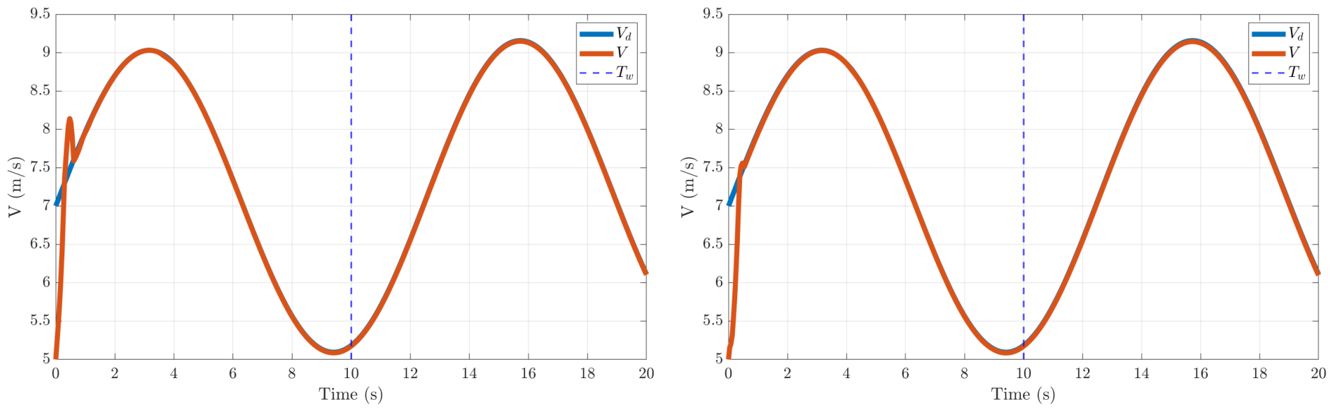
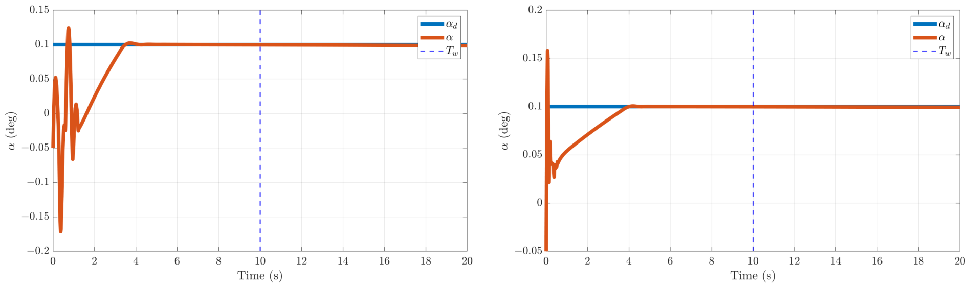
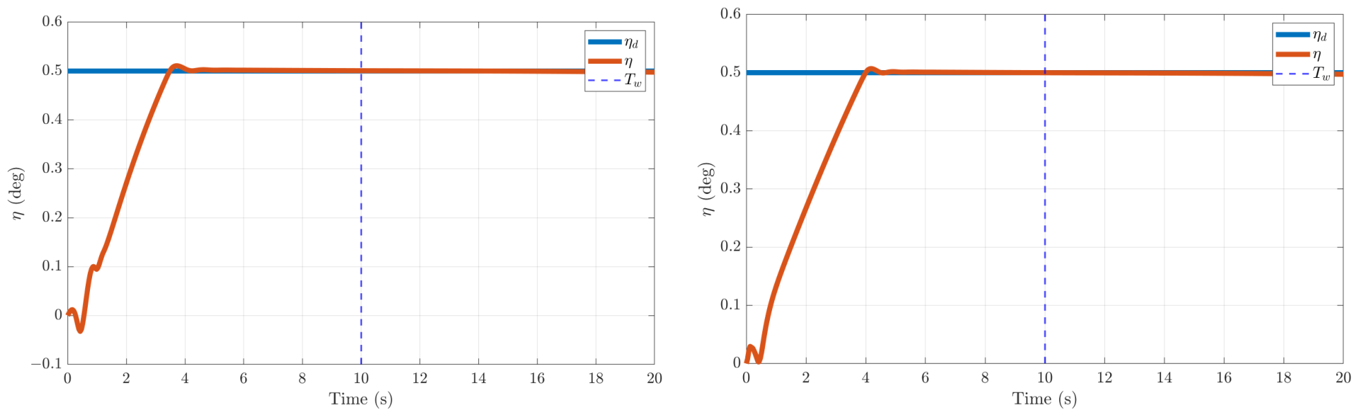
Figure 3, Figure 4 and Figure 5 compare the tracking performance of the two parameter sets for velocity, angle of attack, and dihedral angle. Both cases show a short initial adjustment followed by bounded tracking. The second parameter set contains stronger pitch-rate and dihedral angle coupling, especially in the fourth row of ${\mathit{A}}_2$ and in the fourth row of ${\mathit{B}}_2$, but the controller still keeps the main rigid and elastic responses close to their commands. This indicates that the zero-sum RL policy addsa degree of robustness to the considered model-parameter variation.

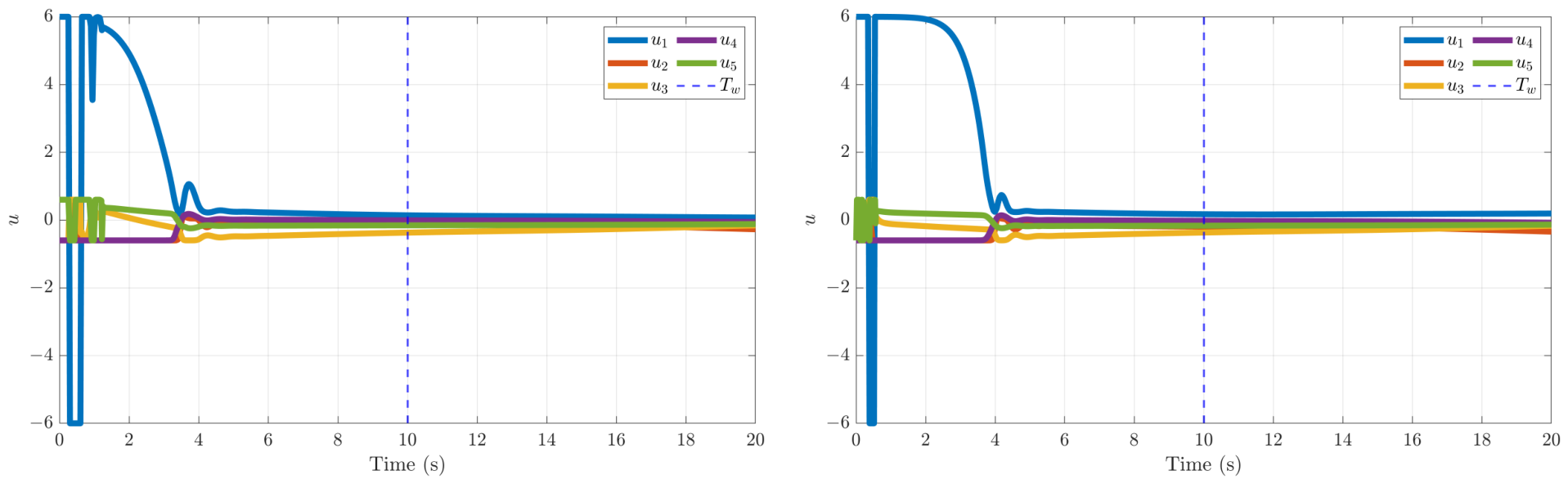
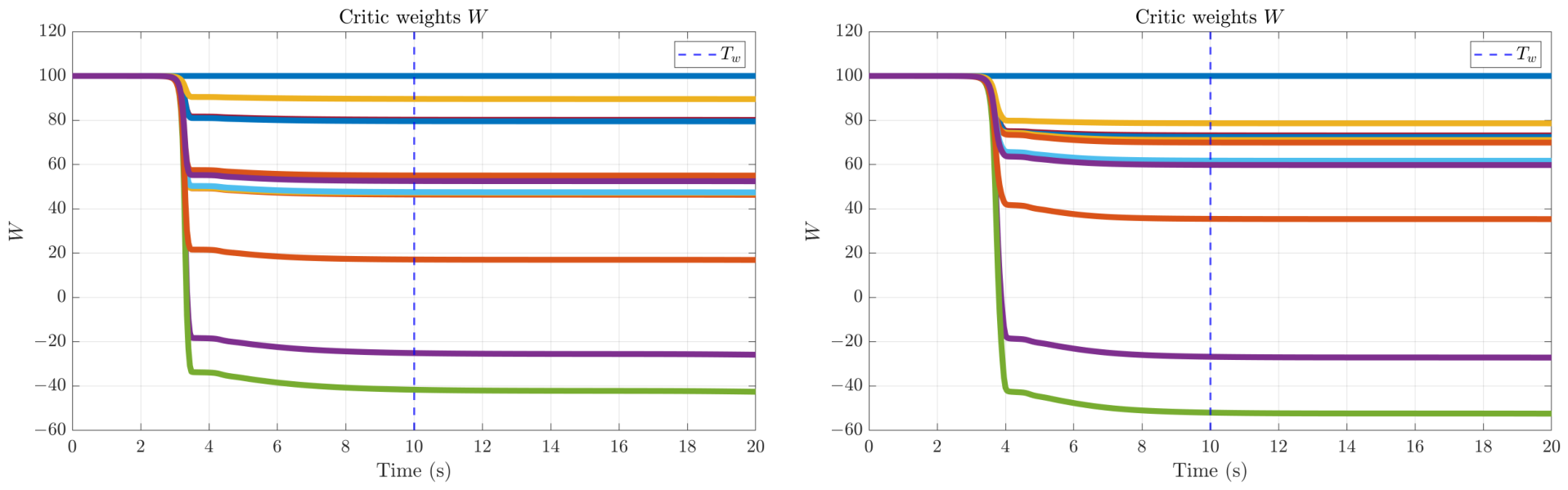
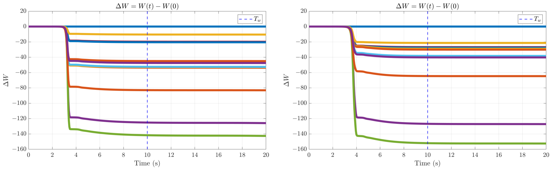
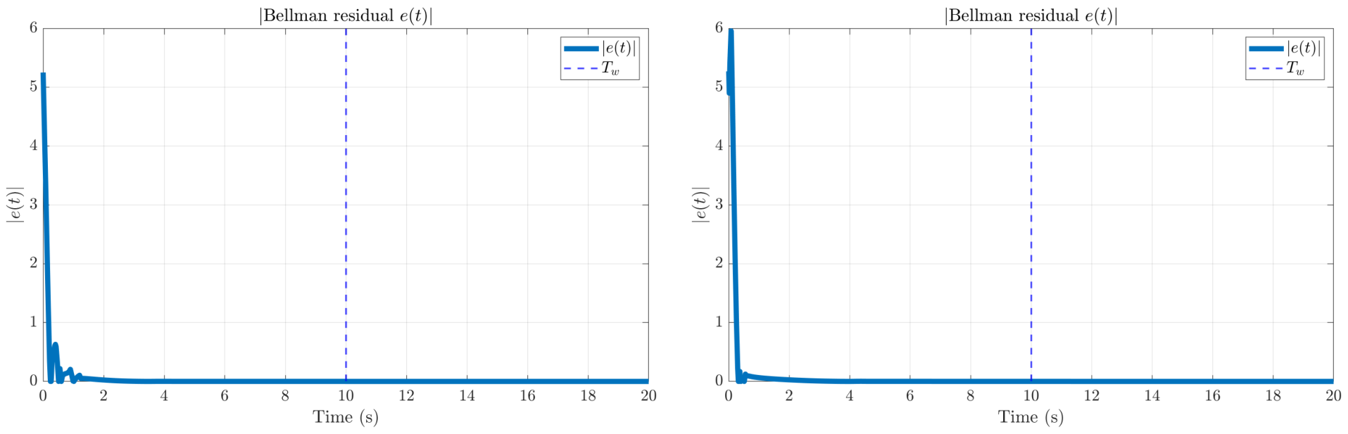
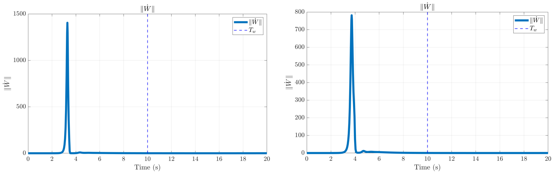
Figure 6 shows that the five control channels remain smooth. Figure 7, Figure 8, Figure 9 and Figure 10 describe the critic-learning process. The critic weights change rapidly during the early learning interval, then remain bounded. The weight increments decrease after the main adaptation phase, showing that the learning process is concentrated around the prescribed learning window. The Bellman residual is not forced exactly to zero because the basis functions and disturbance estimate are approximate, but it stays bounded in both cases. The weight-update norm also decreases after the initial transient, which supports the practical predefined-time critic convergence stated in Theorem 1.

Overall, the two-case simulations verify three points. First, the zero-sum controller suppresses bounded disturbances. Second, the predefined-time critic update concentrates learning activity within the prescribed time window and keeps the Bellman residual bounded afterward. Third, the same controller parameters work for both HFA parameter sets, which indicates robustness to the considered model-parameter variation.

5.2. Comparison with Traditional Methods

In this section, the proposed algorithm is compared with traditional Integral Reinforcement Learning (IRL) algorithms introduced by Ma [32]. The linearized state matrix and input matrix is $({\mathit{A}}_2,{\mathit{B}}_2)$, which is introduced in the previous section. $T_w$ is $5 \mathrm{s}$, and other simulation conditions are the same as the previous section.

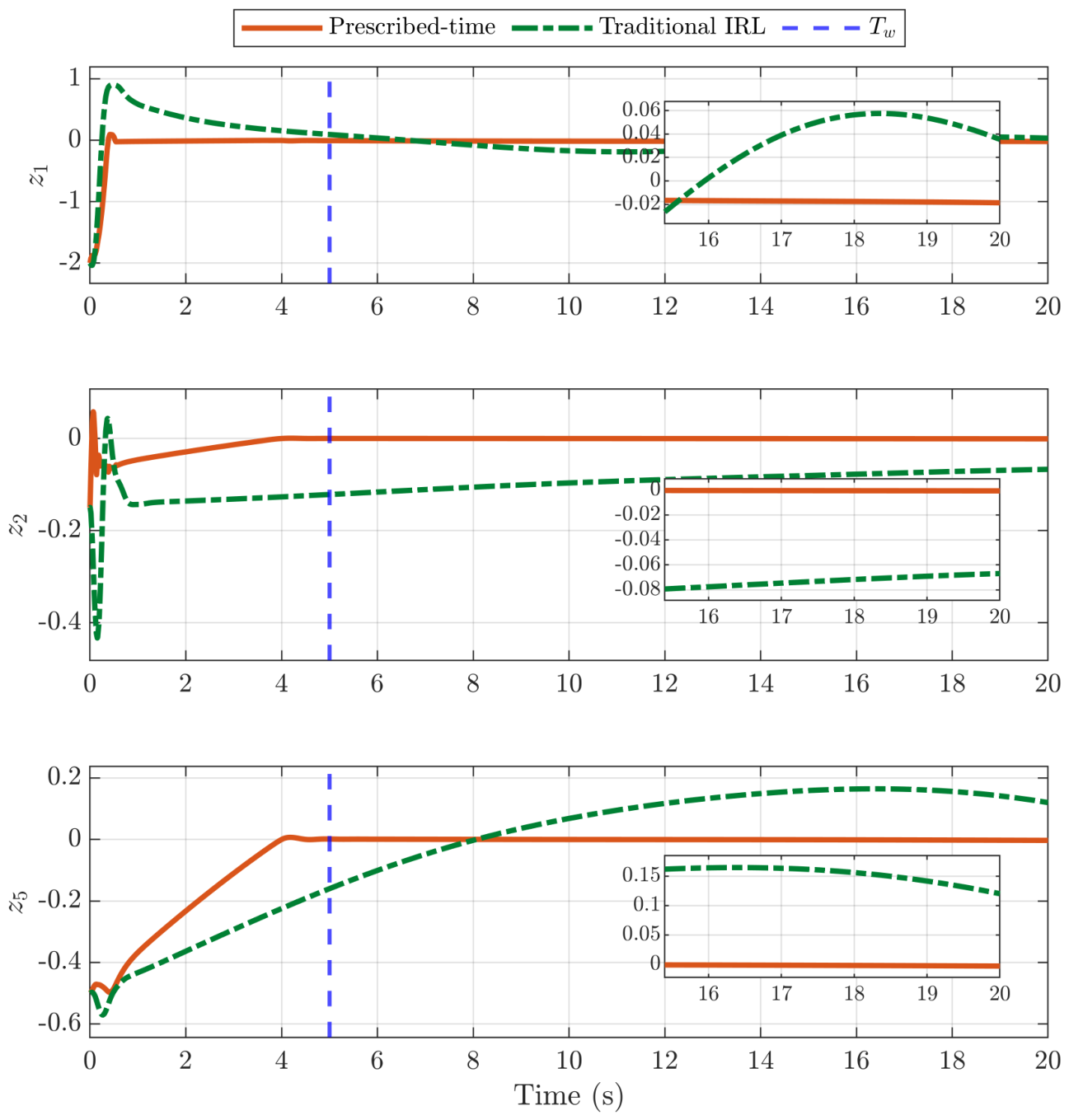
Based on the simulation results presented in the figures, a comparative analysis between the proposed method and the conventional nominal Integral Reinforcement Learning (IRL) approach reveals significant performance advantages of the former. The superiority of the proposed method is primarily evidenced by its rapid convergence characteristics and high-precision tracking capabilities.

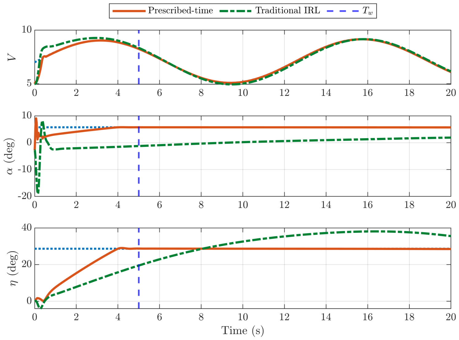
As illustrated in the state trajectory plots in Figure 11, the proposed controller demonstrates a markedly faster transient response compared to the nominal IRL method. Specifically, for states $\alpha$ and $\eta$, the proposed method achieves convergence to the desired reference values within approximately $4\mathrm{s}$. In contrast, the nominal IRL method exhibits a sluggish response, failing to reach the steady-state target, even after $20\mathrm{s}$ of operation. This indicates that the prescribed-time framework effectively overcomes the asymptotic convergence limitations often associated with traditional adaptive or learning-based controllers, guaranteeing system stabilization within a user-defined timeframe independent of initial conditions.

The tracking-error dynamics further corroborate the robustness of the proposed scheme in Figure 12. While the nominal IRL method maintains non-negligible steady-state errors, the proposed method drives tracking errors $z_1$, $z_2$, and $z_5$ to zero with high precision. The error trajectories for the proposed method remain virtually flat at zero after the settling time, whereas the nominal IRL shows continuous drift or offset, highlighting the superior disturbance rejection and parameter-estimation accuracy of the proposed algorithm.

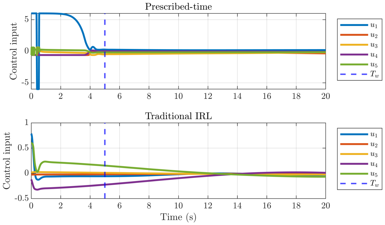
Regarding the control input activity in Figure 13, although the proposed method initially utilizes higher control authority to enforce the fast convergence, it settles to a stable equilibrium rapidly within 5 s. Conversely, the nominal IRL method applies significantly smaller control magnitudes but fails to stabilize the system effectively, resulting in prolonged transient periods. This trade-off suggests that the proposed method efficiently utilizes available control energy to achieve superior dynamic performance, whereas the nominal method’s conservative input leads to inadequate system regulation.

In summary, the comparative results validate that the proposed control method offers substantial improvements over the nominal IRL method, particularly in terms of convergence rate, steady-state accuracy, and transient response quality.

5.3. Model Uncertainty

In this section, model uncertainty is introduced to assess the robustness of the algorithm proposed in this paper. The linearized state matrix and input matrix is $({\mathit{A}}_2,{\mathit{B}}_2)$, which is introduced in the previous section. The linearized system has eigenvalues with ${\lambda }_1=-7.11$, ${\lambda }_2=-0.019$, ${\lambda }_{3,4}=-0.016\pm 0.64i$, and ${\lambda }_{5,6}=-4.82\pm 18.66i$ [32]. The system-matched uncertainties are caused by flexible effects of dihedral angle [33].

In the simulation environment, ${\mathit{A}}_{real}$ replaces $\mathit{A}$ in the calculation of environmental information feedback, when the proposed algorithm has no information about it and still uses $\mathit{A}$ in the calculation of controller, where

$${\mathit{A}}_{real}=\mathit{A}+\Delta \mathit{A}$$

(101)

Different $\Delta \mathit{A}$ values are settled as follows:

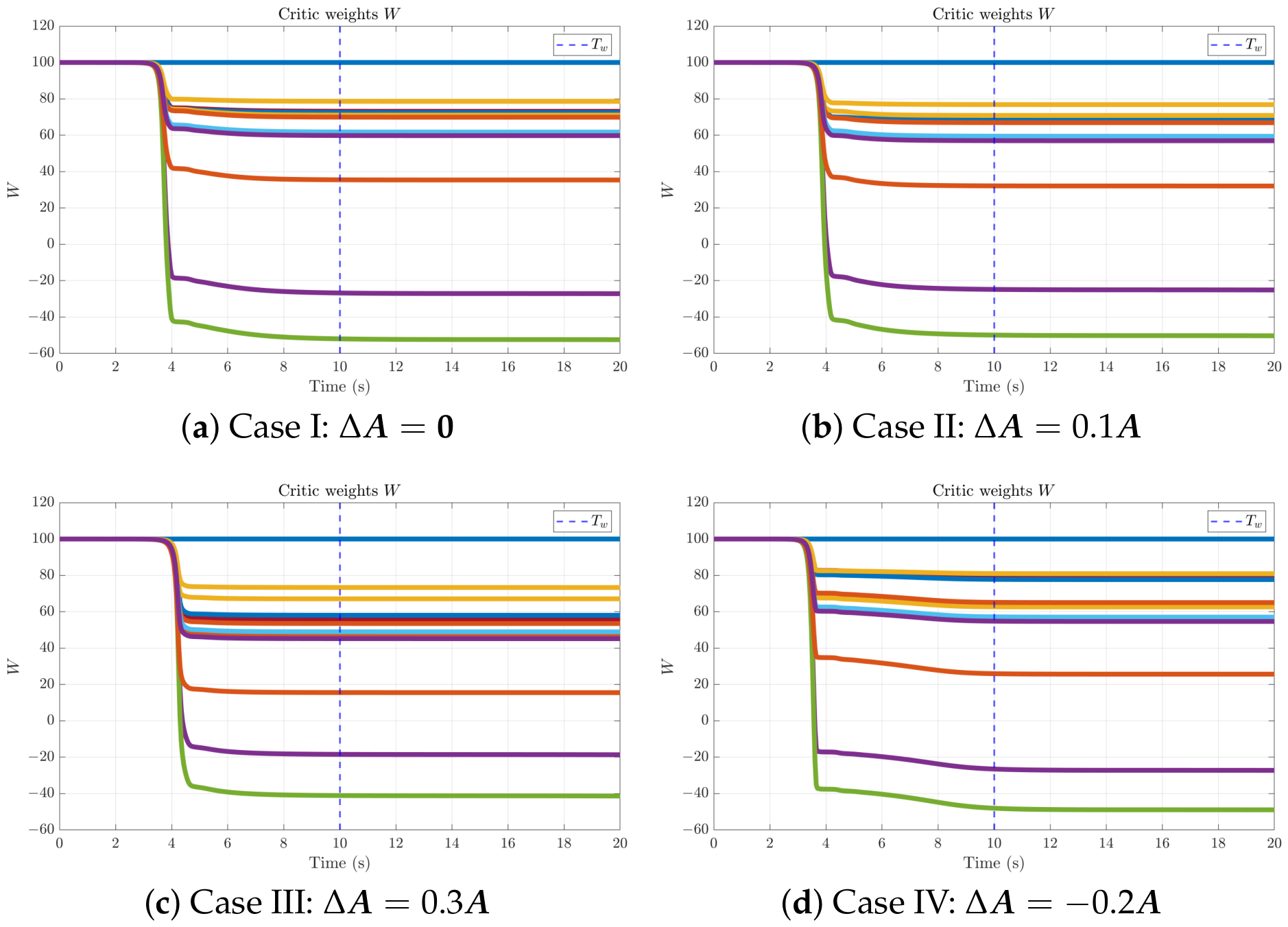
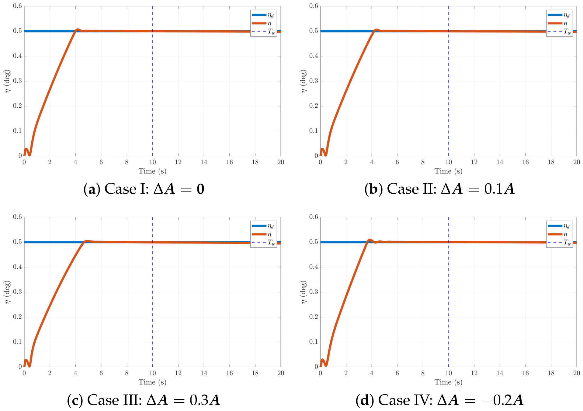
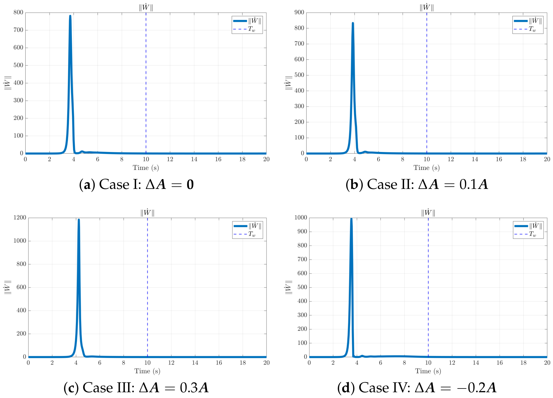
Case I: no model uncertainty, $\Delta \mathit{A}=\mathbf{0}$;

Case II: low model uncertainty, $\Delta \mathit{A}=0.1\mathit{A}$;

Case III: high model uncertainty, $\Delta \mathit{A}=0.3\mathit{A}$

Case IV: negative model uncertainty, $\Delta \mathit{A}=-0.2\mathit{A}$.

Other simulation conditions are the same as in the previous section.

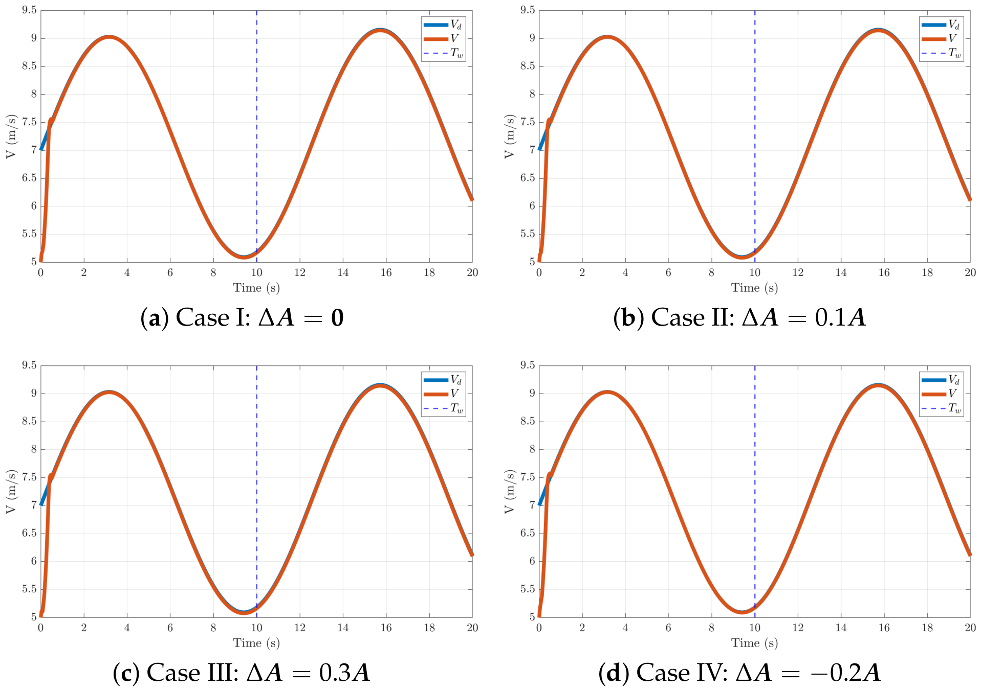
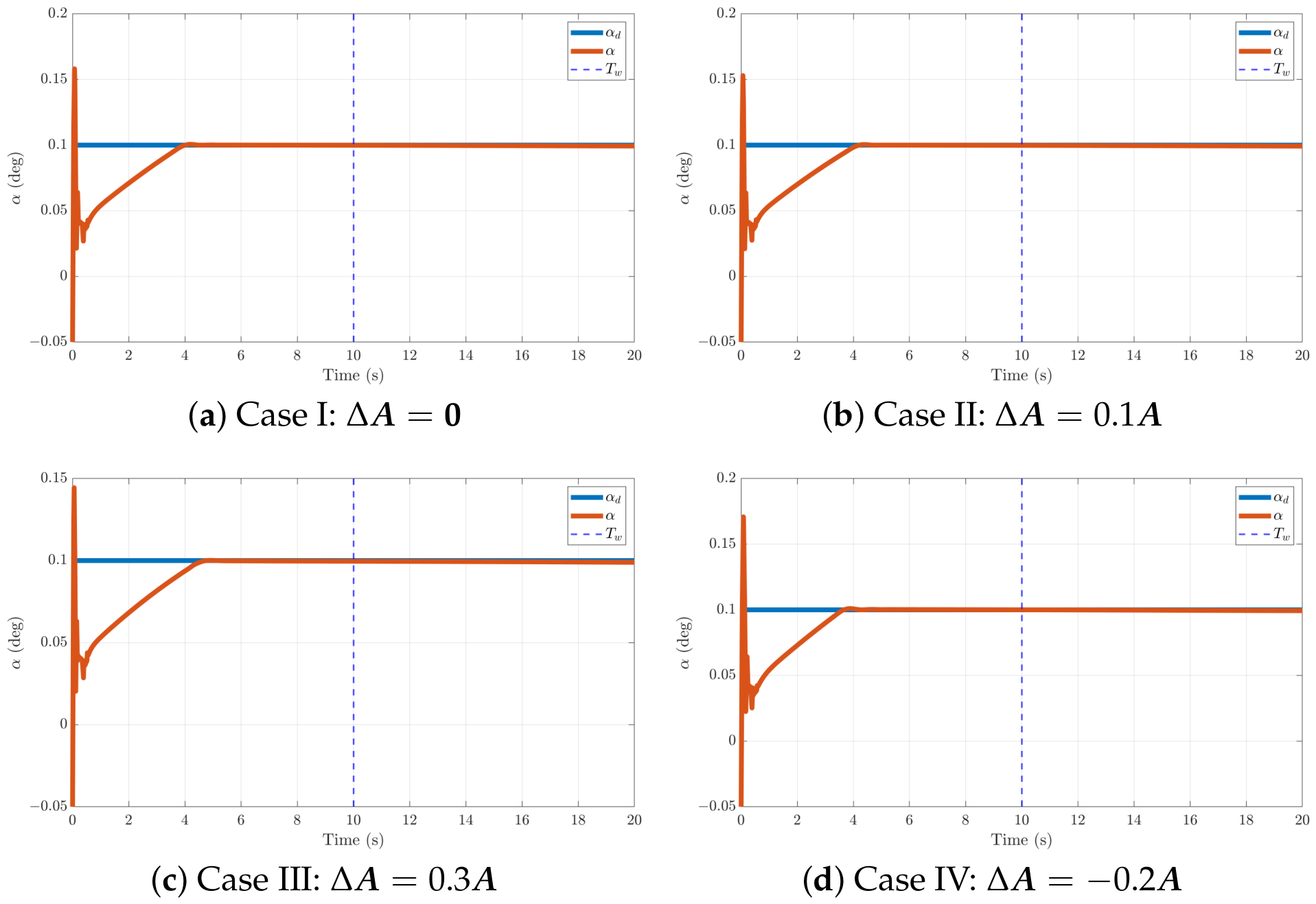
Figure 14, Figure 15 and Figure 16 demonstrate that the proposed controller preserves essentially invariant tracking performance across all tested uncertainty levels. The commanded and measured trajectories overlap closely after a short transient of approximately 4–5 s, with negligible steady-state error and nearly identical rise and settling times, irrespective of the sign or magnitude of $\Delta \mathit{A}$.

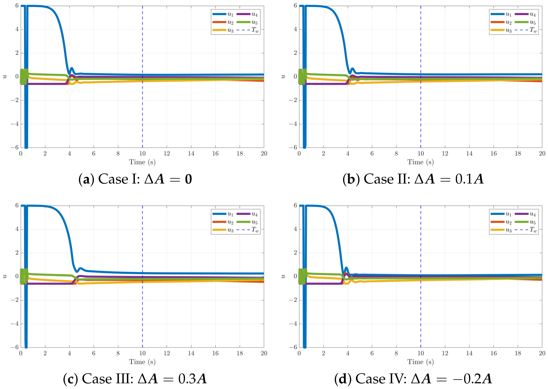
Under the same uncertainty cases, the control inputs remain bounded, smooth, and free of saturation or sustained oscillations in Figure 17. The transient profiles and peak amplitudes are nearly indistinguishable across $\Delta \mathit{A}$, and no chattering is observed; input rates stay within acceptable limits, indicating benign actuation demands and strong robustness of the control law.

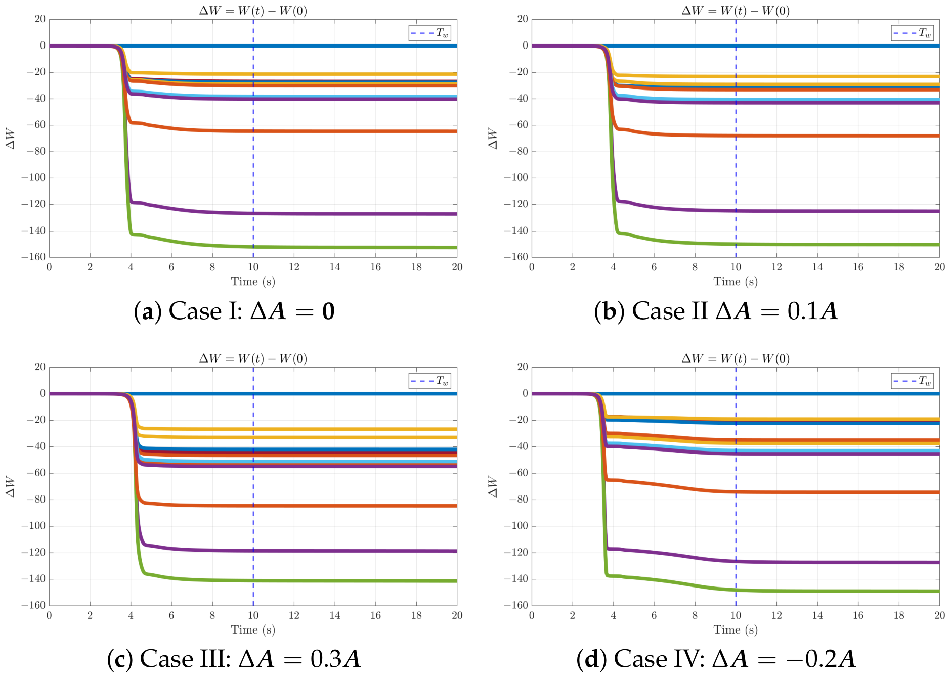
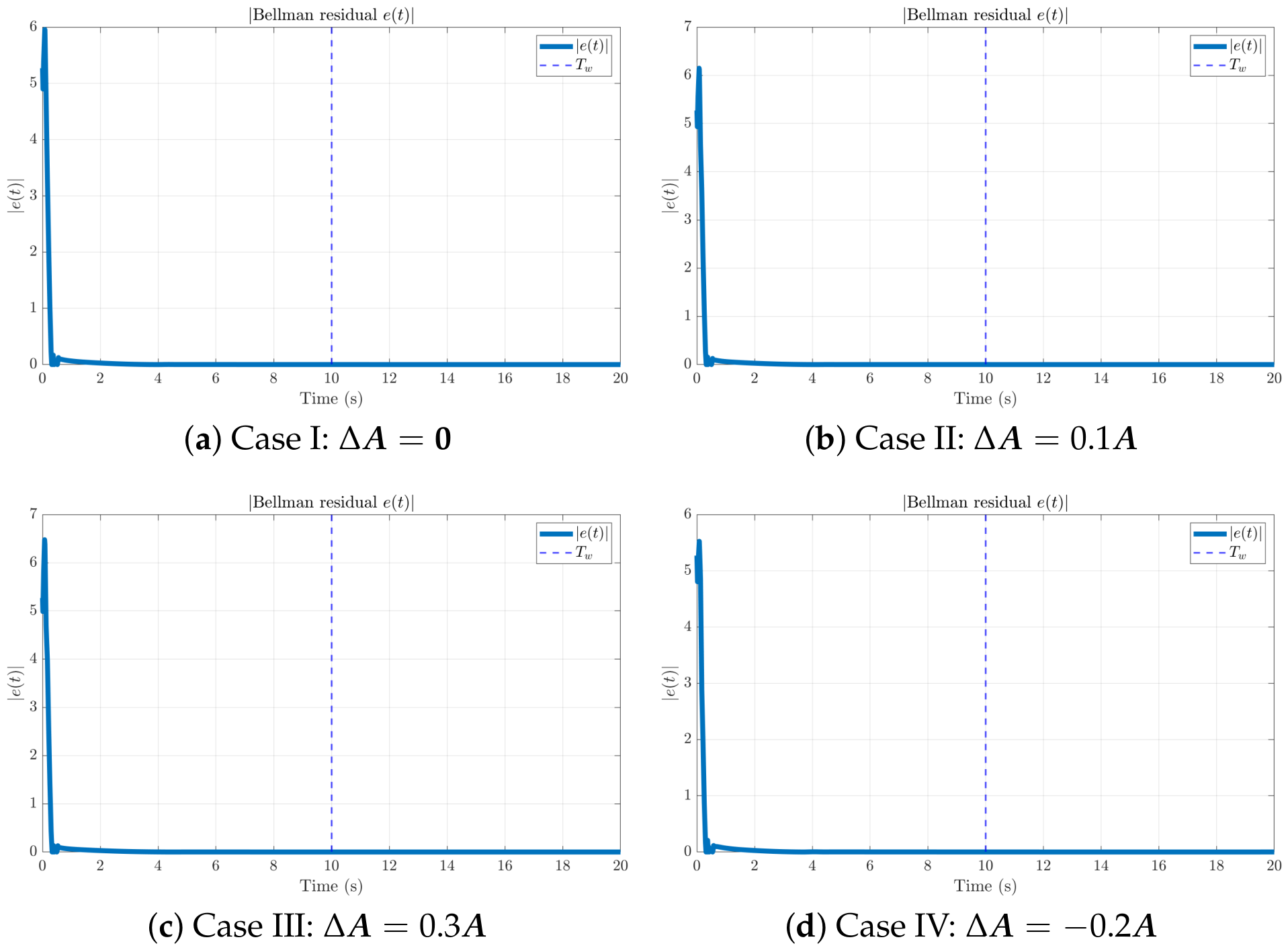
Figure 18, Figure 19, Figure 20 and Figure 21 characterize the learning process. The critic weights converge to bounded constants, the weight-update increments rapidly decay to small values, and the Bellman residual drops by several orders of magnitude and stays near zero. The norm of the weight-update vector exhibits an early peak, then quickly vanishes. Closed-loop performance is preserved, even after learning is frozen at $T_w$, evidencing stable adaptation and insensitivity to modeling errors up to every tested $\Delta \mathit{A}$.

5.4. Measurement Noise

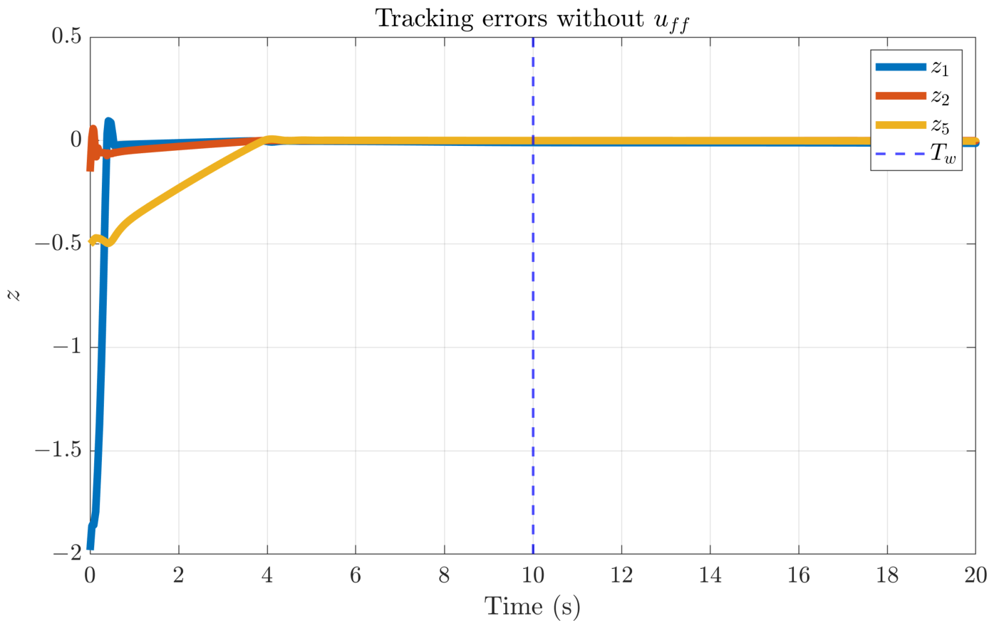
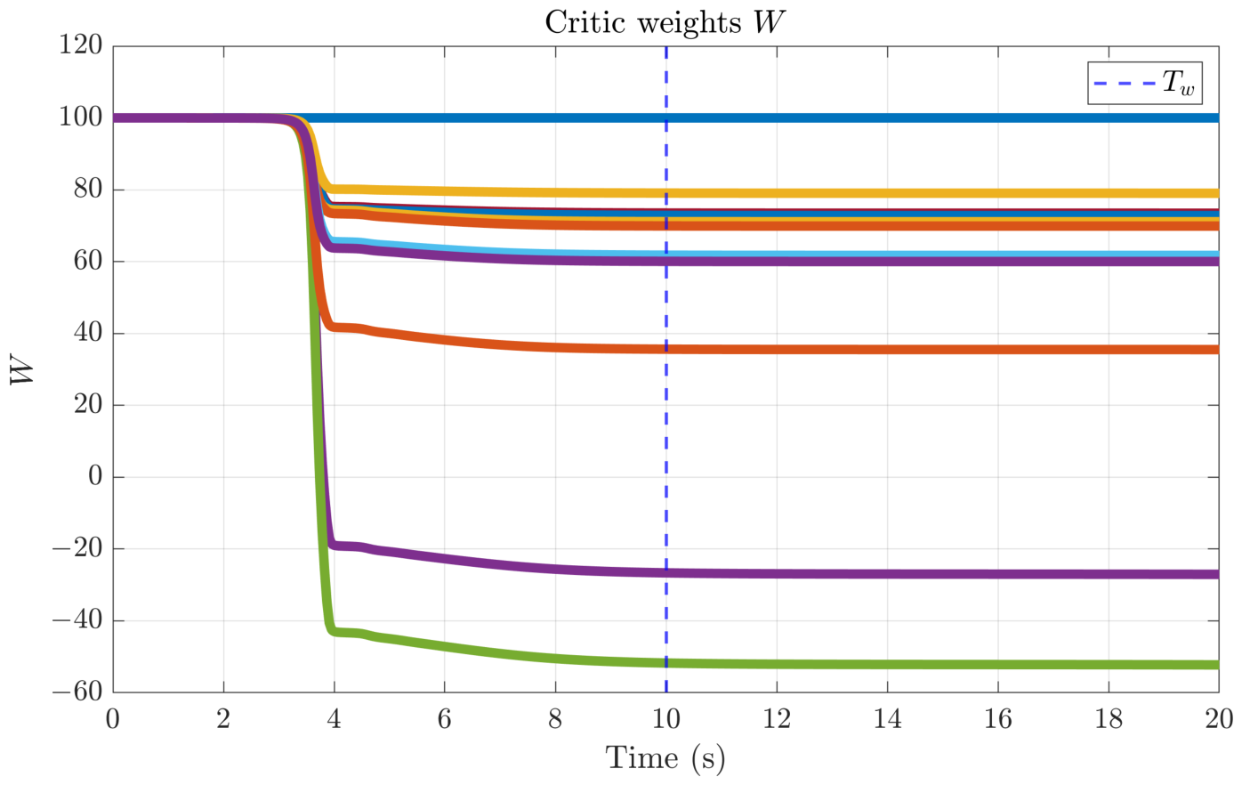
The measurement noiseis represented as

$${\mathit{x}}_m\left(t\right)=\mathit{x}\left(t\right)+\mathit{n}\left(t\right),$$

(102)

where $\mathit{n}\left(t\right)={\left[0.02\cos \left(0.1t\right),0.005\sin \left(0.5t\right),0.005\sin \left(0.1t\right),0.005\cos \left(0.5t\right),0.005\sin \left(0.1t\right),0.005\cos \left(0.5t\right)\right]}^{\top }$ denotes the measurement-noise vector. The resulting tracking errors and critic-weight responses are given below.

Figure 22 and Figure 23 present the results in the presence of measurement noise. The tracking errors remain bounded and decrease to a small neighborhood of zero after a short transient, while the critic weights exhibit bounded learning responses and gradually approach steady values before $T_w$. Therefore, the introduced measurement noise does not significantly degrade the tracking performance across tested measurement-noise levels.

6. Conclusions

This paper presented a practical predefined-time reinforcement learning method for robust tracking control of highly flexible aircraft. A zero-sum differential-game formulation was used to model the interaction between the tracking controller and the worst-case disturbance. A critic neural network was introduced to approximate the Hamilton–Jacobi–Isaacs equation solution online, and a fractional-power update law was developed to make the critic weight-estimation error converge to a bounded neighborhood within a prescribed learning time. A composite Lyapunov analysis established uniform ultimate boundedness of the coupled closed-loop system. Different trim-point experiments based on two HFA parameter sets demonstrated that the proposed method can achieve bounded tracking under external sinusoidal disturbances. Comparison with traditional IRL methods demonstrated the superiority of the proposed method. Model-uncertainty experiments demonstrated the method proposed in this paper performs well under different model uncertainties. Zero-sum game-based practical predefined-time reinforcement learning control for highly flexible aircraft with actuator saturation and time delay is an important direction for future work.