Transferability of Quantum Feature Maps from Simulation to Hardware in Healthcare Data

Abstract

Quantum machine learning is often proposed for richer feature representations, yet most evidence rests on idealized simulation rather than real noisy intermediate-scale quantum (NISQ) hardware. This research presents a controlled comparison of classical and quantum-enhanced diagnostic pipelines on three clinical binary classification tasks: Mammographic Mass, Anemia, and Diabetic Retinopathy. All pipelines share standardized preprocessing, principal component analysis (PCA), and a fixed extreme gradient boosting (XGBoost) classifier, so differences arise only from the feature representation. Four quantum encodings (angle, phase, basis, and the ZZ feature map) are each run on two backends: a noiseless simulator and the real IBM Heron r2 processor (156 qubits). Across nine performance metrics, compared with the classical pipeline, the performance decreases in the quantum hardware execution for all datasets, with a more significant reduction observed for the Anemia dataset. In contrast, compared with the simulated pipeline, the hardware execution shows a slight performance decrease for the Mammographic and Diabetic Retinopathy datasets. The exceptions are the angle and phase encodings for the Mammographic dataset, where the hardware result improves slightly compared with the simulator. For the Anemia dataset, the transition from simulation to real quantum hardware results in a considerable performance reduction. These findings show that current quantum feature maps through the encode–measure–boost pipeline on NISQ hardware do not yet outperform a well-designed classical pipeline.

1. Introduction

1.1. Background

Early and accurate diagnosis of disease remains one of the central challenges of modern healthcare, because the difference between a timely intervention and a missed one is often the difference between recovery and irreversible harm. Clinical screening data for conditions such as breast cancer, anemia, and diabetes are typically tabular in nature, consisting of a modest number of numerical and categorical measurements per patient. On such data, machine learning (ML) classifiers must extract subtle, often non-linear relationships between features, yet the feature interactions that separate a healthy patient from an at-risk one are frequently faint and overlapping. Conventional pipelines respond to this difficulty by engineering features by hand or by compressing them linearly, but these representations can flatten precisely the higher-order dependencies that carry diagnostic signal. This motivates a search for richer feature representations that can expose hidden structure in clinical data without demanding larger datasets, and quantum feature map has recently emerged as one such candidate [1,2].

In 2022, breast cancer alone was responsible for an estimated 2.3 million new cases and 670,000 deaths worldwide and was the most common cancer among women in 157 of 185 countries [3]. Anemia is even more prevalent, with an estimated 1.9 billion people (~24% of the world’s population) living with anemia in 2021, making it the third largest cause of disability globally [4]. Diabetes rounds out this picture. The 11th edition of the IDF Diabetes Atlas reports that in 2024 an estimated 589 million adults were living with the disease, about one in nine, and the disease was responsible for around 3.4 million deaths in a single year [5]. The three combined conditions affect billions of lives, and a small improvement in the accuracy of automated screening translates into a meaningful number of patients correctly flagged for care. In the face of such monumental and growing clinical burden, our methodological question is how best to represent medical data for diagnosis.

1.2. Motivation and Research Summary

To address this question, this research designs and compares two parallel diagnostic pipelines applied to three benchmark medical datasets, namely the Mammographic Mass, Anemia, and Diabetic Retinopathy, each treated as a binary classification problem. Both pipelines share an identical foundation so that any difference in performance can be attributed cleanly to the feature representation rather than to incidental choices. In every case, the raw data are first standardized using scaling and reduced through principal component analysis (PCA), and the extreme gradient boosting (XGBoost) classifier with a fixed random state of 42 is used as the common downstream model to guarantee reproducibility. The first pipeline serves as a classical baseline, feeding the PCA-reduced features directly into XGBoost. The second pipeline inserts a quantum feature map stage between dimensionality reduction and classification, transforming the classical features into quantum-derived representations before the same XGBoost classifier consumes them. The quantum feature map stage itself is realized through four distinct encoding strategies, each capturing a different facet of the data. These are angle encoding, basis encoding, phase encoding, and ZZ feature map. Crucially, each quantum encoding is executed on two complementary backends so that our findings are not an artifact of an idealized environment. This research first runs every circuit on a noiseless classical simulator, and then re-runs the identical circuits on real IBM Heron r2 quantum hardware. Comparing simulated and hardware results side by side allows us to assess not only whether the quantum feature map helps, but also whether its benefits survive the realities of present-day quantum devices.

1.3. Major Contributions

Before presenting the main contributions, it is important to clarify what is new in this study. Although quantum feature maps, quantum kernels, and the effects of noise have been widely studied, this work does not propose a new encoding or optimization method. Instead, it examines how different quantum encodings perform when the same experimental setup is evaluated on both an ideal simulator and a real quantum processor. Unlike many previous studies, all major components, including preprocessing, feature reduction, data partitioning, classifier settings, and encoding circuits, are kept unchanged, while only the computational backend is varied. This design helps distinguish the effect of the encoding from the effect of real hardware noise. It also allows the performance of each encoding to be related to its circuit complexity and evaluated across different datasets. Importantly, the study reports cases where quantum encoding does not improve performance, which provides useful insight into its practical limitations. These results provide a clearer understanding of how different quantum feature maps affect performance in healthcare tabular data. Thus, the key contributions of this work are:

• Controlled classical–quantum benchmarking: This research presents a controlled comparison between classical and quantum-enhanced diagnostic pipelines, where preprocessing, dimensionality reduction, and classification remain identical, isolating the effect of feature representation alone.
• Simulation-to-hardware adaptability assessment: This research evaluates the adaptability of quantum feature maps from noiseless simulation to real IBM Heron r2 quantum hardware, which quantifies the impact of NISQ noise on diagnostic performance and identifies practical limitations for current healthcare applications.
• Circuit complexity, error, and computational cost analysis: This study evaluates the resource requirements of different quantum feature maps, including gate counts, circuit depth, and error-related factors. It also compares their computational costs to provide a clearer understanding of how circuit complexity and hardware errors may influence overall performance.

In the next part of this paper, Section 2 presents the existing works related to this research, Section 3 introduces the datasets and preliminary concepts of the research, Section 4 outlines the proposed method, Section 5 details the results and discussion of this research, and finally, Section 6 concludes the research.

2. Related Works

A significant theme in the quantum data-driven healthcare method is that the performance of the classification is highly dependent on how the classical data are represented prior to learning. Hossain et al. [6] demonstrated this clearly in chronic kidney disease diagnosis, where PCA-based optimization performed far better than singular value decomposition (SVD). PCA gave an accuracy of 98.75% for classical support vector machine (SVM) and 87.5% for quantum SVM (QSVM). The accuracy of QSVM dropped drastically to 60% with SVD. This result suggested that quantum classifiers were very sensitive to the quality of feature representation and could lose performance when the transformed features did not preserve meaningful diagnostic structure. Such a concern was also raised in the breast cancer study by Genç [7], where quantum feature-map-based transformation was compared to classical models. The classical SVM and logistic regression reached 96.49% accuracy, while the quantum-transformed model with all features reached 98.25% accuracy. However, when only the top five selected features were used, the accuracy was 94.74%. This outcome demonstrated that quantum feature maps could improve diagnostic performance, but too much feature reduction could lead to the exclusion of valuable information for accurate classification. Hossain et al. [8] also analyzed the feature map techniques and their circuit depth in their research. They tested three feature maps, namely SOE, Z, and ZZ, with different circuit depths in multiple datasets and found that the classification performance depended on the selection of both a suitable feature map and an appropriate depth. In a lung cancer study, Toufah et al. [9] compared three feature maps, namely Z, ZZ and Pauli, and reported that the Pauli feature map had the strongest performance, including perfect classification in three balanced subsets. Yadav et al. [10] proposed a hybrid QSVM and quantum neural network (QNN) model for breast cancer diagnosis using Z, ZZ and Pauli feature maps. Their model achieved accuracy of over 90% and improvement in both classification performance and computational cost. The hybrid structure was significant because QSVM provided kernel-based robustness and QNN offered trainable variational feature extraction. However, their work was mostly based on a simulator and still needed to be validated on more powerful real quantum machines. Munshi et al. [11] applied QSVM and a variational quantum circuit (VQC) for the prediction of heart failure in healthcare 4.0. In their results, they showed that QSVM outperformed VQC with 82% accuracy. Although lower than many classical healthcare models, the accuracy was useful because the work demonstrated the practical use of quantum ML (QML) classifiers on a real medical prediction dataset. The authors also mentioned that the main obstacles for QML-based healthcare systems were hardware instability, limited number of qubits and difficulty in parameter optimization. Ahmad et al. [12] developed a hybrid quantum-classical machine learning model to predict whether a person working in the technology sector may require future mental health treatment. They encoded classical survey data into a quantum feature space using the Z and ZZ feature maps, then trained a QSVM and compared its performance against a classical SVM. Finally, they executed the same quantum model on both a simulator and real IBM quantum processors to evaluate the practicality of QML on current NISQ hardware. Singh and Pokhrel [13] systematically studied the impact of different quantum noise models on QML algorithms for genome classification. They observed that QSVM was more robust to noise than Pegasos QSVM and QNN, but some feature maps, especially the Pauli feature map, were extremely susceptible to depolarizing and amplitude-damping noise. This study showed that performance in the feature map could vary widely in the presence of noise.

3. Dataset and Preliminaries

This section provides the empirical basis on which proposed research pipelines are built and evaluated. Section 3.1 describes the datasets, and Section 3.2, Section 3.3 and Section 3.4 present the preliminaries to prepare and evaluate them.

3.1. Dataset

To evaluate the robustness and generalizability of quantum feature maps, this research conducts experiments on three publicly available benchmark datasets. These datasets differ substantially in dimensionality and class distribution, which enables assessment under diverse data characteristics. A brief description of each dataset is provided below.

• Mammographic Mass: The first dataset is the Mammographic Mass dataset [14]. This dataset is used for early diagnosis of breast cancer by predicting the benign or malignant status of a mammographic mass. It comprises 830 patient records described by five attributes: breast imaging reporting and data system (BI-RADS) assessment, patient age, and three morphological descriptors of the mass (its shape, margin and density). The prediction target, severity, is a binary label with the value of one for a malignant mass and the value of zero for a benign mass. The dataset is fairly balanced, with 427 benign and 403 malignant cases. This is a good candidate for a fair binary classification study, as the classifier is not biased towards a dominant class. The small number of features makes it a natural starting point for dimensionality reduction and quantum encoding, where the width of the quantum circuit is given by the number of retained components.
• Anemia: The second dataset is the Anemia dataset [15]. It consists of 1421 records, described by five features drawn from a routine complete blood count, namely the patient’s gender plus four red-blood-cell indices: hemoglobin concentration, mean corpuscular hemoglobin (MCH), mean corpuscular hemoglobin concentration (MCHC) and mean corpuscular volume (MCV). The target variable, Result, specifies if a patient has anemia or not. There are 620 anemics and 801 non-anemic cases. This leads to a slight class imbalance with respect to the mammographic data, but the dataset is still sufficiently balanced for the training to be reliable, and the larger sample size provides a more challenging test of whether quantum-derived representations still separate the classes as the volume of data increases.
• Diabetic Retinopathy: The third dataset is the Diabetic Retinopathy dataset [16], which represents the diabetes-related screening task and is by far the most complex of the three in terms of dimensionality. It consists of 1151 records extracted from retinal images, each described by nineteen attributes that summarize image quality, the results of pre-screening, a series of detected microaneurysm counts at varying confidence levels, several exudate-based lesion measurements, and geometric descriptors such as the distance between the macula and the optic disk and the diameter of the optic disk. The binary target, class, denotes whether signs of Diabetic Retinopathy are present, comprising 611 positive and 540 negative cases and forming an approximately balanced problem. The high dimensionality of this dataset makes it especially valuable for the present study, since it most clearly exposes the role of dimensionality reduction and reveals how each feature map strategy behaves when many correlated measurements must be compressed before encoding.

Together, these three datasets cover a range from low to high dimensionality and from screening for oncological and hematological conditions to ophthalmic conditions. By treating each as a binary classification problem within the same pipeline, the study can examine not only whether quantum feature map offers improved performance but also whether any such improvement is consistent across clinically diverse problems.

3.2. Principal Component Analysis (PCA)

In this work, PCA is used for two complementary purposes. It first addresses the redundancy in clinical data, where measures are often correlated. Instead of removing correlated features, it combines them into composite components, so that the diagnostic content of related features is preserved instead of being discarded. Second, and importantly for the quantum pipeline, the number of principal components retained determines the number of qubits required for each feature map, since each component is encoded onto a single qubit. This reduces the feature space to circuits that are shallow enough for current quantum hardware while keeping the parts that focus the variance most likely to improve classification accuracy. Specifically, we retain four main components for the Mammographic Mass dataset, five main components for the Anemia dataset, and seven main components for the Diabetic Retinopathy dataset. PCA does not simply throw away individual features, but it constructs each principal component as a weighted linear combination of the original features. PCA orders the components such that the first captures as much variance as possible in the data, the second captures as much of the remaining variance as possible subject to being orthogonal to the first, and so on. Thus, redundant information dispersed across several correlated measurements is compressed into a few informative directions, and the dimensionality of the data can be reduced with minimal loss of the variance that carries the discriminative signal [17,18].

Formally, given a standardized data matrix whose covariance matrix is Σ, PCA solves the eigenvalue problem:

Σv_i = λ_iv_i

(1)

where each eigenvector v_i defines the direction of a principal component and its associated eigenvalue λ_i quantifies the variance captured along that direction. The components are then ranked in descending order of their eigenvalues, and the projection of an original sample x onto the leading k components yields the reduced representation:

z = W^⊤ (x − μ)

(2)

where μ is the mean of the data and W is the matrix whose columns are the k leading eigenvectors. The resulting vector z is the compact, decorrelated feature representation that is passed either directly to the classifier in the baseline pipeline or onward to the quantum feature-mapping stage.

3.3. Feature Map

Feature map is the process of transforming the PCA-reduced classical features into a quantum state, so that the data are represented in the high-dimensional Hilbert space associated with a system of qubits. The motivation is that a quantum feature map can embed the data in a space whose dimension grows exponentially with the number of qubits, where relationships that are entangled and non-linear in the original representation may become more readily separable. Because no single encoding is optimal for every dataset, and because the literature shows that the choice of feature map interacts strongly with the structure of the data, this study employs four complementary strategies, namely angle encoding, phase encoding, basis encoding, and the ZZ feature map [19,20]. Each captures a different facet of the data, ranging from individual feature magnitudes to explicit pairwise interactions, and comparing them allows the analysis to identify which form of quantum representation, if any, benefits a given clinical problem. In all four maps, the encoded value of each component is scaled by π so that the normalized features span a meaningful range of rotation angles, and neighboring qubits are entangled through a linear chain of controlled-NOT gates that couples component i with component i + 1. The following explains each feature map used in this research in detail.

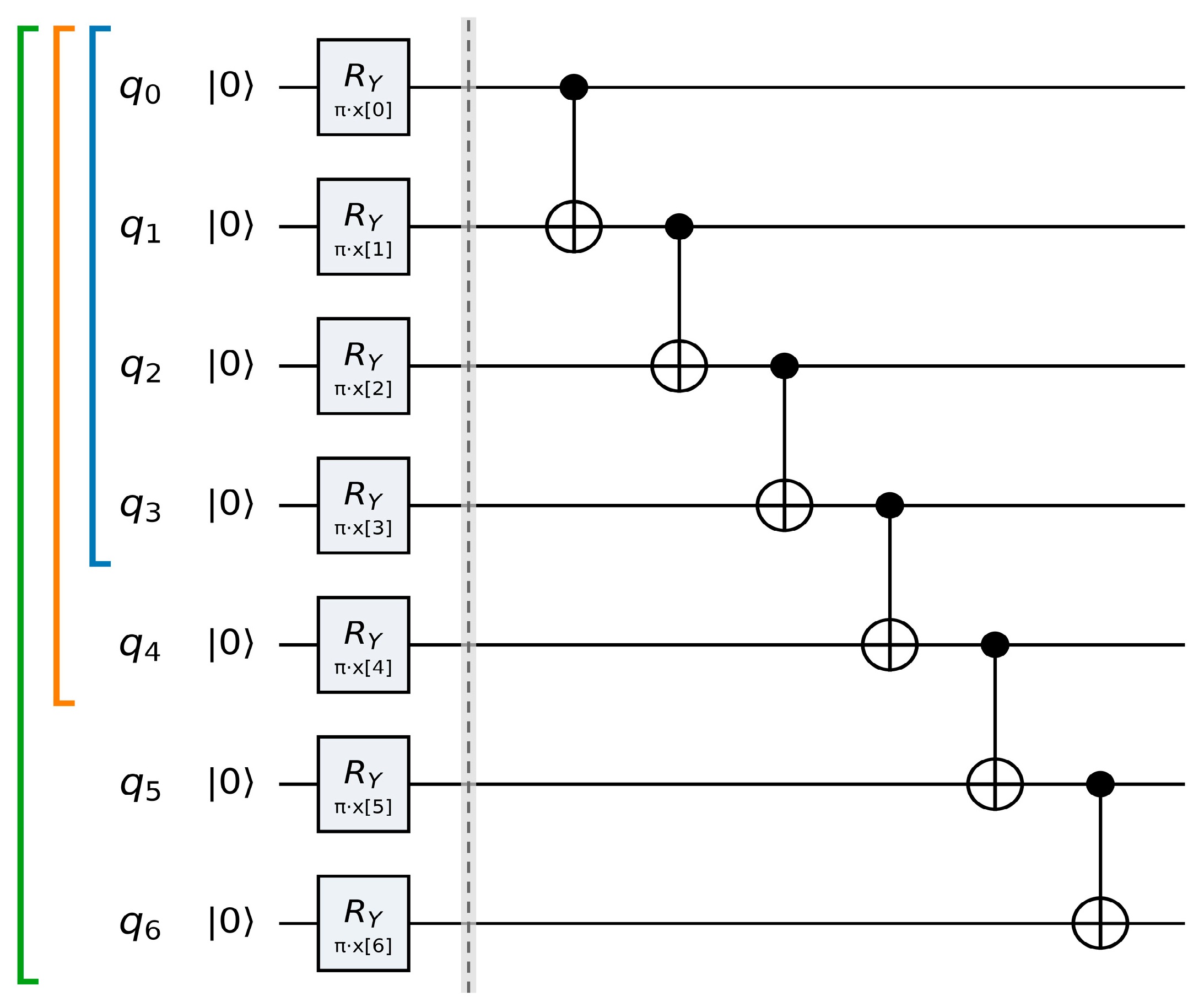
• Angle encoding: Figure 1 shows the angle-encoding circuit used in this research. Angle encoding maps each normalized feature directly onto the rotation angle of a single qubit. For every component x_i, a rotation about the Y axis is applied with an angle proportional to the feature value, after which a linear chain of CNOT gates entangles adjacent qubits so that the individual feature magnitudes and their interactions are preserved together. The single-qubit operation is
  R_Y(θ_i) |0〉, θ_i = x_i × π

  (3)

  so that a feature value near zero leaves the qubit close to its ground state while a value near one rotates it toward the excited state, giving a direct and interpretable embedding of feature magnitude into qubit amplitude [21].

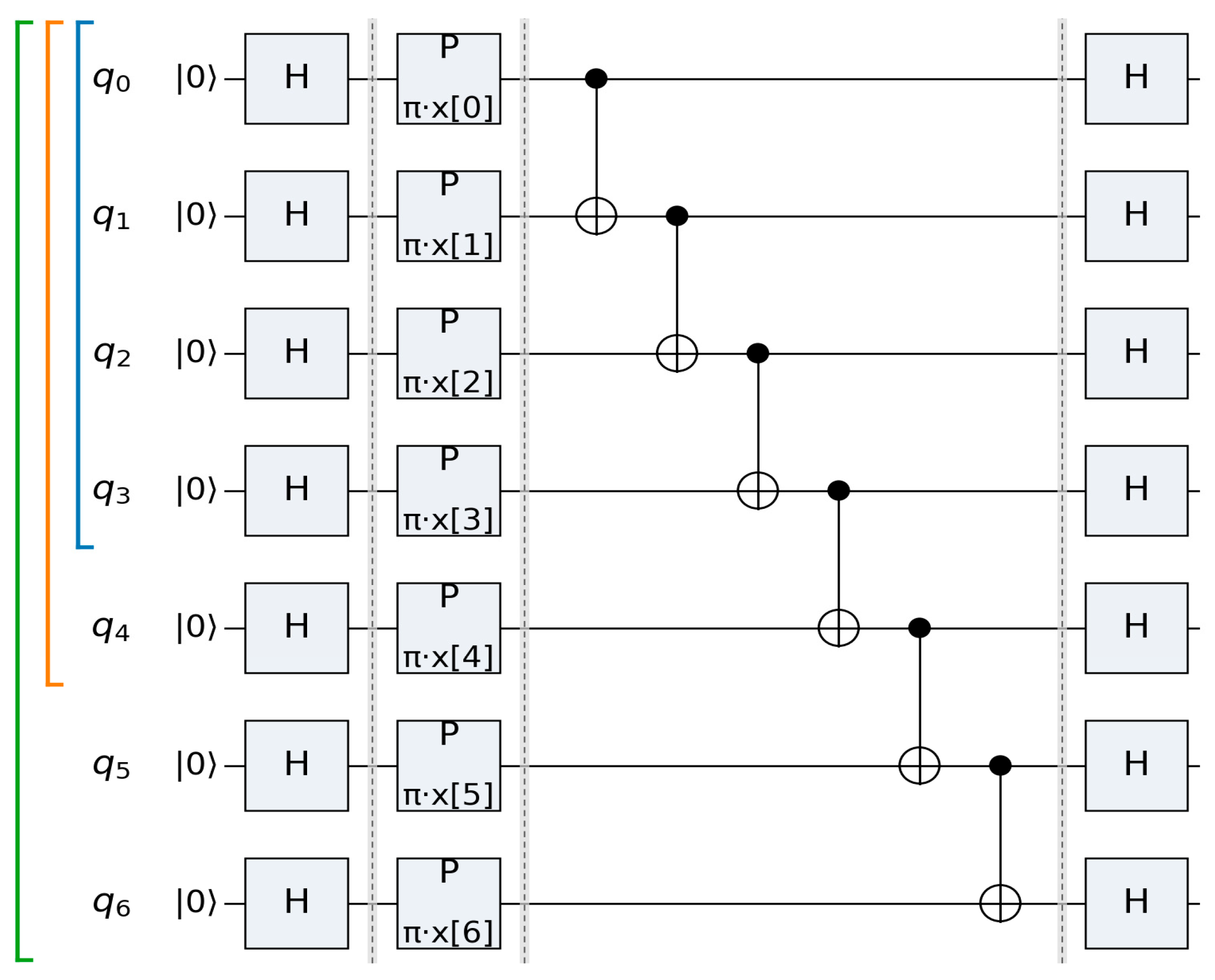
• Phase encoding: Figure 2 shows the phase-encoding circuit used in this research. Phase encoding instead stores each feature in the phase of the quantum state rather than in its amplitude. Each qubit is first placed in an equal superposition by a Hadamard gate; a phase-shift gate then imprints the feature value as a relative phase, a linear chain of CNOT gates introduces entanglement, and a final Hadamard layer converts the accumulated phase information into measurable probability differences. The phase-shift gate applied to qubit i is,
  P(θ_i), θ_i = x_i × π

  (4)

  By encoding information in the phase and only later interfering it back into the computational basis, this map can expose non-linear patterns that are not directly visible in the raw feature amplitudes [22].

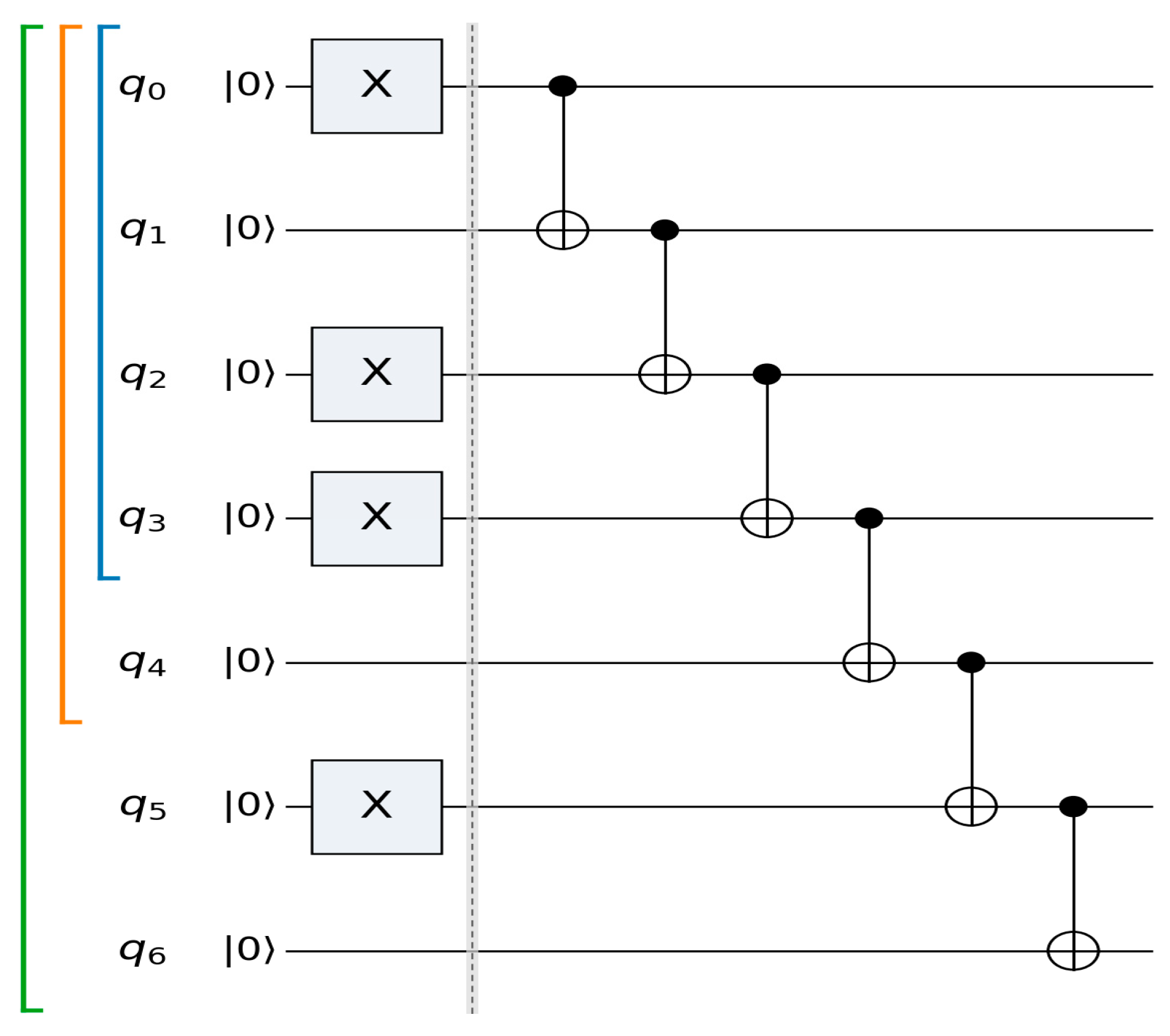
• Basis encoding: Figure 3 presents the basis-encoding circuit used in this study. Basis encoding maps classical data directly onto computational basis states. Each normalized component is binarized around a threshold of 0.5. If the binarized value is equal to one, a Pauli-X gate is applied to the corresponding qubit, then the same linear CNOT entanglement is added. The binarization rule is
  b_i = 1 if x_i ≥ 0.5, otherwise b_i = 0

  (5)

  with the qubit prepared as |bi〉. This yields a deliberately simple representation that captures threshold-crossing behavior and provides a discrete counterpart against which the continuous encodings can be compared [23].

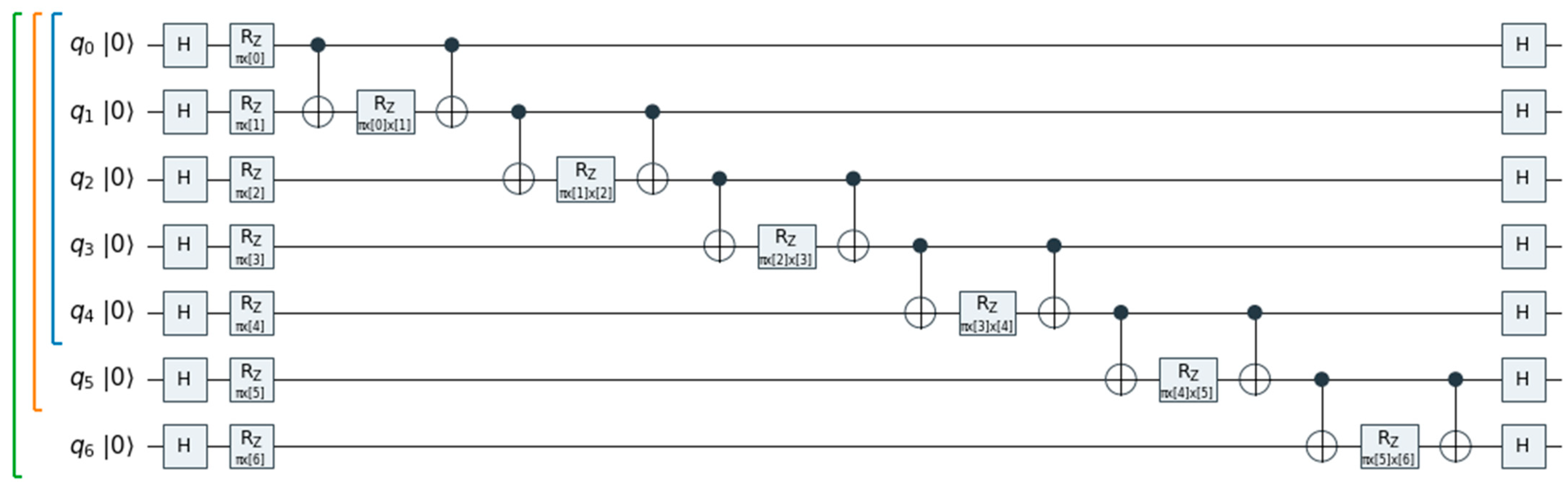
• ZZ feature map: Figure 4 shows the ZZ feature map circuit used in this research. The ZZ feature map encodes feature-to-feature interactions explicitly rather than relying on entanglement alone to couple them. After a Hadamard layer creates superposition, each feature is encoded through a single-qubit R_Z rotation, and a sequence of two-qubit blocks then entangles each adjacent pair of qubits and applies a further rotation whose angle depends on the product of the two corresponding feature values. After all neighboring interactions have been encoded, a final Hadamard layer is applied to every qubit to convert the accumulated phase information into amplitudes that can be observed in the computational basis. The single-qubit and interaction angles are
  θ_i = x_i × π, θ_zz = x_i × x_i+1 × π

  (6)

  where each interaction term is realized by a CNOT gate, an R_Z rotation by θzz, and a second CNOT. The final Hadamard layer completes the feature map by enabling interference among the encoded quantum phases before measurement. By writing the pairwise products of features directly into the quantum state, the ZZ feature map represents higher-order dependencies that the other encodings can only capture implicitly, at the cost of a deeper circuit that is more sensitive to hardware noise [24].

3.4. Assessment Metrics

To classify the data, this research uses the classical XGBoost [25] model. XGBoost is often chosen because it combines high predictive performance with built-in regularization and also efficiently handles complex non-linear relationships, feature interactions, and diverse data types. Since the main purpose of this research is to observe the transferability of the quantum feature map from classical healthcare data to quantum representations rather than building an accurate structure, this research selects the adaptable XGBoost model as a ground to assess the effectiveness of each feature map.

Classification quality is measured through the different classified counts of each class. True positives (TP) measure the number of actual positive instances classified as positive, while true negatives (TN) represent the number of actual negative instances classified as negative; false positives (FP) measure the number of actual negative instances classified as positive, and false negatives (FN) measure the number of actual positive instances classified as negative. Based on these counts, the performance metrics are described as follows [26,27,28,29].

• Accuracy (Ac.): It measures the overall proportion of classes classified correctly and offers a single headline figure of merit. It is defined as:

$$\mathrm{A}\mathrm{c}={\displaystyle \frac{(\mathrm{T}\mathrm{P}+\mathrm{T}\mathrm{N})}{\mathrm{T}\mathrm{P}+\mathrm{T}\mathrm{N}+\mathrm{F}\mathrm{P}+\mathrm{F}\mathrm{N}}}$$

(7)

• Precision (Pr.): It evaluates the accuracy of positive predictions by measuring the proportion of predicted positive instances that are correctly classified. This metric is especially relevant when the cost of false positive errors is high. It is defined as:

$$\mathrm{P}\mathrm{r}={\displaystyle \frac{\mathrm{T}\mathrm{P}}{\mathrm{T}\mathrm{P}+\mathrm{F}\mathrm{P}}}$$

(8)

• Recall (Re.): This metric is also known as the true-positive rate (TPR). It is the percentage of truly positive classes the model correctly identifies. It is calculated as:

$$\mathrm{R}\mathrm{e}={\displaystyle \frac{\mathrm{T}\mathrm{P}}{\mathrm{T}\mathrm{P}+\mathrm{F}\mathrm{N}}}$$

(9)

• F1-score (F1.): This score is a single measure that combines precision and recall, calculated as their harmonic mean. It is informative because it penalizes models that sacrifice one for the other. It is given by:

$$\mathrm{F}1=2\times {\displaystyle \frac{\mathrm{P}\mathrm{r}\times \mathrm{R}\mathrm{e}}{\mathrm{P}\mathrm{r}+\mathrm{R}\mathrm{e}}}$$

(10)

• Specificity (Sp.): This measurement measures the ability of a classifier to correctly identify negative instances by quantifying the proportion of actual negative instances that are correctly classified as negative. It is defined as:

$$\mathrm{S}\mathrm{p}={\displaystyle \frac{\mathrm{T}\mathrm{N}}{\mathrm{T}\mathrm{N}+\mathrm{F}\mathrm{P}}}$$

(11)

• Cohen’s Kappa (Ka.): It measures the level of agreement between the predicted and actual class labels while accounting for the agreement that may occur by chance. It provides a more robust assessment of classification performance than simple accuracy, particularly when the class distribution is imbalanced. Let (po) denote the observed agreement and (pe) denote the agreement expected by chance. Then it is defined as:

$$\mathrm{K}\mathrm{a}={\displaystyle \frac{\mathrm{p}\mathrm{o}-\mathrm{p}\mathrm{e}}{1-\mathrm{p}\mathrm{e}}}$$

(12)

• ROC-AUC (Ra.): The receiver operating characteristic area under the curve (ROC-AUC) evaluates the ability of a classifier to distinguish between positive and negative classes across all possible decision thresholds. It is computed as the area under the ROC curve, which plots the TPR against the false positive rate (FPR). An ROC-AUC value of 1 indicates perfect discrimination, whereas a value of 0.5 indicates performance equivalent to random guessing. It is expressed as:

$$\mathrm{R}\mathrm{a}={\int }_0^1\mathrm{T}\mathrm{P}\mathrm{R}\left(\mathrm{F}\mathrm{P}\mathrm{R}\right)\mathrm{d}\left(\mathrm{F}\mathrm{P}\mathrm{R}\right)$$

(13)

• PR-AUC (Pa.): The precision–recall area under the curve (PR-AUC) measures the overall performance of a classifier by calculating the area under the precision–recall (PR) curve, which plots precision against recall across all classification thresholds. This metric is particularly useful for imbalanced datasets because it focuses on the classifier’s ability to correctly identify positive instances without being influenced by the large number of negative instances. A higher PR-AUC value indicates better performance in detecting the positive class. It is expressed as:
  $$\mathrm{P}\mathrm{a}={\int }_0^1\mathrm{Precision}\left(\mathrm{Recall}\right)\mathrm{d}\left(\mathrm{Recall}\right)$$

  (14)

  To ensure a reliable performance evaluation, all experiments are conducted using 5-fold cross-validation, and the overall performance is reported by mean values. For each fold, PCA is fitted using only the training data and then applied to the corresponding test data to prevent information leakage. Besides the above performance metrics, the 95% confidence interval (95% CI) is calculated for the accuracy to quantify the variability and statistical reliability of the obtained results. The 95% CIs are calculated from the mean and standard deviation of the accuracy values obtained across the five cross-validation folds.

4. Methodology

The main design principle is controlled comparison, meaning that all pipelines ingest the same datasets, apply the same preprocessing and the same PCA and end in the same XGBoost classifier described in Section 3. So, the only quantity allowed to vary is the way the data are represented before classification. In this common scaffold, three pipelines are built, and Section 4.1, Section 4.2 and Section 4.3 present them in detail.

4.1. Classical Pipeline

This baseline is used to compare with simulation and real quantum hardware approaches of quantum feature map. As shown in Figure 5, this baseline consists of four sequential stages that begin from the raw dataset, which in each case is one of the three benchmark collections introduced in Section 3.1. However, the scales, units and dimensionality of these clinical tables are different. The next step is a common preprocessing procedure to clean and standardize the data. In this step, we deal with missing or inconsistent entries and rescale each feature so that no attribute dominates the subsequent analysis just because it is measured on a larger numerical range. The standardized features are then fed to the PCA stage, formally described in Section 3.2, which re-expresses the possibly correlated clinical measurements as a smaller set of mutually uncorrelated principal components. PCA, as said, has a twofold aim: it concentrates the discriminative variance of several correlated features into a few informative directions, and it fixes the dimensionality of the representation; it keeps four components for the Mammographic Mass dataset, five for the Anemia dataset and seven for the Diabetic Retinopathy dataset. Finally, the PCA-reduced features are supplied to an XGBoost classifier. Finally, the PCA-reduced features are supplied to an XGBoost classifier, and the classified data are then evaluated through the metrics of Section 3.4. The classical pipeline therefore answers the question of how well the data can be classified using only a conventional linear reduction.

4.2. Quantum Simulated Pipeline

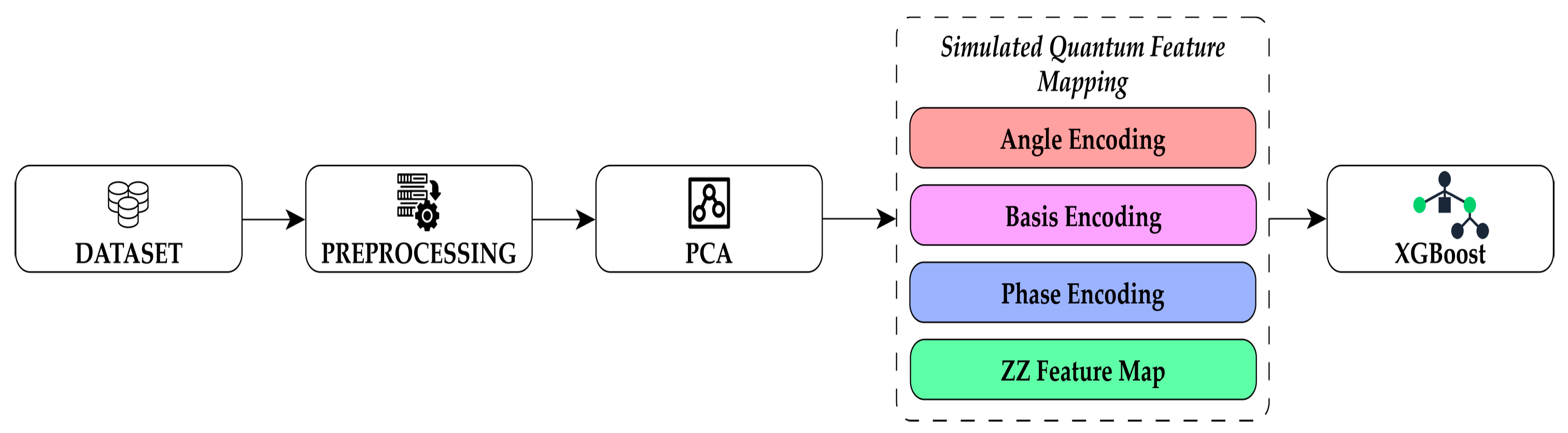
The quantum-simulated pipeline introduces the central idea of the study: the quantum feature map. As illustrated in Figure 6, the dataset, preprocessing, PCA, and XGBoost stages are exactly those of the classical pipeline, except the quantum feature map stage. In the feature map stage, the four principal components of the mammographic data, the five of the anemia data, or the seven of the retinopathy data are taken as the inputs to a quantum circuit, where each component is encoded onto a single qubit. The encoding is carried out using the four strategies defined in Section 3.3, namely angle encoding, basis encoding, phase encoding, and the ZZ feature map. For each feature map, the transformed quantum data is then evaluated by XGBoost. After execution of each quantum feature map circuit, all qubits are measured in the computational basis. The resulting measurement counts are normalized by the total number of shots to obtain the probability distribution over all computational basis states. For the noiseless simulation, the same 500 shots per circuit used in the hardware experiments are applied to obtain the measurement counts that ensure the simulation and hardware results use the same finite-shot sampling budget. This normalized probability vector constitutes the quantum-derived feature representation supplied to the XGBoost classifier. Consequently, the dimensionality of the input to XGBoost is 2ⁿ, where n is the number of retained principal components. Therefore, the Mammographic Mass, Anemia, and Diabetic Retinopathy datasets generate feature vectors of dimensions 16, 32, and 128, respectively. The same readout protocol is applied to both the noiseless simulator and the IBM Heron r2 (IBM, USA) hardware of Section 4.3 to ensure a consistent comparison.

In the simulated pipeline, every feature map circuit is executed on a noiseless idle classical simulator, which uses 500-shot sampling, consistent with the hardware experiments, to obtain the resulting measurement counts and without any of the errors that affect physical hardware. The simulation-based pipeline enables the evaluation of quantum representations under ideal operating conditions. This approach isolates the effect of the feature map itself and reveals the intrinsic representational capability of each feature map when quantum operations are executed without errors.

4.3. Quantum Hardware Pipeline

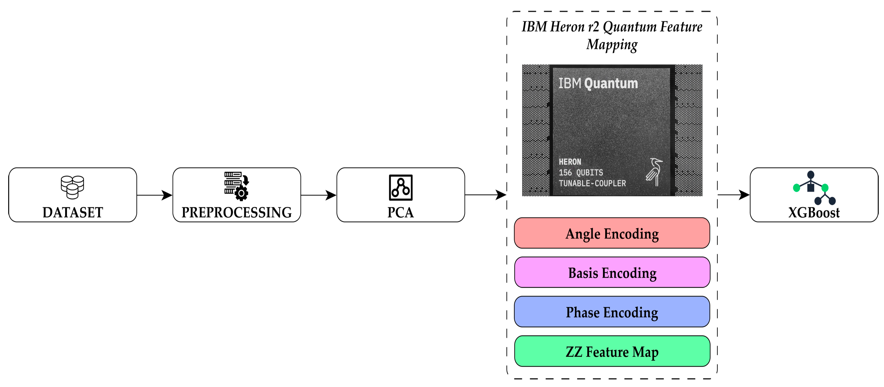
As depicted in Figure 7, the third pipeline follows the same framework as the quantum simulation pipeline described in Section 4.2, with one important distinction: the feature map circuits used to encode the classical data into quantum states are executed on real quantum hardware rather than on an ideal simulator. For this purpose, the IBM Heron r2 quantum processor, a 156-qubit device based on a tunable-coupler architecture, is employed. Executing the feature maps on physical quantum hardware exposes the circuits to the inherent limitations of current noisy intermediate-scale quantum (NISQ) systems, including gate errors, qubit decoherence, readout inaccuracies, and crosstalk between neighboring qubits. These hardware-induced effects are intrinsic to real quantum devices and cannot be fully captured by idealized simulations. Consequently, this pipeline provides a practical assessment of whether the representational benefits observed under noise-free simulation remain effective when the same quantum circuits are implemented on an actual quantum processor.

The hardware pipeline experiments are performed on the IBM Quantum backend ibm_kingston using 500 shots per circuit. Transpilation is performed using target = backend.target with an optimization level of 1, while qubit mapping and routing are handled automatically. The Mammographic Mass, Anemia, and Diabetic Retinopathy datasets used 4, 5, and 7 logical qubits, respectively. No error-mitigation technique is applied, and Qiskit version 2.5.1 is used. Because both the simulator and hardware experiments use 500 shots per circuit, finite-shot sampling is controlled across the two backends. Therefore, the observed differences between simulation and hardware primarily reflect hardware noise and execution-related effects [30,31].

5. Results and Discussion

5.1. Performance Assessment

Table 1. Outcome of the classical pipeline.

Dataset	Ac.	Pr.	Re.	F1.	Ra.	Pa.	Sp.	Ka.	95% CI
Mammographic	0.8024	0.7975	0.8041	0.7989	0.8795	0.8636	0.8013	0.6050	±0.0444
Anemia	0.9880	0.9903	0.9823	0.9862	0.9998	0.9998	0.9925	0.9757	±0.0114
Diabetic Retinopathy	0.6125	0.6375	0.6267	0.6316	0.6637	0.7203	0.5963	0.2228	±0.0257

summarizes the overall outcome of the classical pipeline. The Anemia dataset achieves the highest performance with an accuracy of 0.9880, precision of 0.9903, recall of 0.9823, and F1-score of 0.9862. It also obtains high values for specificity (0.9925) and kappa score (0.9757), with a narrow 95% confidence interval of ±0.0114. The Mammographic dataset provides moderate results with an accuracy of 0.8024, an F1-score of 0.7989, and a kappa value of 0.6050, while the 95% confidence interval is ±0.0444. The Diabetic Retinopathy dataset shows lower performance, with an accuracy of 0.6125, an F1-score of 0.6316, and a kappa value of 0.2228.

Table 2. Performance of the quantum simulated pipeline on a noiseless simulator.

Dataset	Encoding	Ac.	Pr.	Re.	F1.	Ra.	Pa.	Sp.	Ka.	95% CI
Mammographic	Angle	0.7783	0.7872	0.7519	0.7677	0.8604	0.8478	0.8036	0.5560	±0.0431
	Basis	0.8145	0.8225	0.7916	0.8058	0.8288	0.7895	0.8363	0.6284	±0.0287
	Phase	0.7759	0.7859	0.7470	0.7641	0.8600	0.8485	0.8036	0.5511	±0.0421
	ZZ	0.7735	0.7804	0.7469	0.7615	0.8498	0.8477	0.7989	0.5462	±0.0649
Anemia	Angle	0.9409	0.9675	0.8952	0.9294	0.9723	0.9769	0.9763	0.8787	±0.0227
	Basis	0.8079	0.7767	0.7871	0.7815	0.8857	0.8176	0.8239	0.6101	±0.0337
	Phase	0.9465	0.9713	0.9048	0.9364	0.9744	0.9778	0.9788	0.8904	±0.0165
	ZZ	0.9388	0.9466	0.9129	0.9287	0.9806	0.9783	0.9588	0.8751	±0.0140
Diabetic Retinopathy	Angle	0.5143	0.5392	0.5842	0.5603	0.5296	0.5607	0.4352	0.0195	±0.0198
	Basis	0.5821	0.6107	0.5956	0.6012	0.5765	0.6098	0.5667	0.1620	±0.0350
	Phase	0.5204	0.5456	0.5875	0.5649	0.5335	0.5616	0.4444	0.0320	±0.0433
	ZZ	0.5334	0.5552	0.6022	0.5771	0.5315	0.5591	0.4556	0.0582	±0.0275

shows the overall outcome of the quantum pipeline when feature map techniques are simulated, where each dataset is evaluated under all four encodings. For the Mammographic dataset, the Basis encoding provides the best performance with an accuracy of 0.8145, an F1-score of 0.8058, a kappa value of 0.6284, and an 95% confidence interval of ±0.0287. The other encoding methods obtain similar accuracy values within the range of 0.7735–0.7783. For the Anemia dataset, all encoding methods achieve strong classification results, where Phase encoding obtains the highest accuracy of 0.9465, an F1-score of 0.9364, and a kappa value of 0.8904. The ZZ encoding also provides competitive performance with an accuracy of 0.9388 and the smallest confidence interval of ±0.0140 among the Anemia results. The Diabetic Retinopathy dataset remains challenging for the quantum pipeline, with accuracy values ranging from 0.5143 to 0.5821 across the encoding methods, where the Basis encoding achieves the highest accuracy (0.5821) and kappa value (0.1620). Compared to the classical in-quantum-simulated pipeline, the overall accuracy increases for the Mammographic dataset with basis encoding, where accuracy decreases for both Anemia and Diabetic Retinopathy datasets.

Executing the quantum feature map circuits on the IBM Heron r2 processor produces the results shown in

Table 3. Performance of the IBM Heron r2 quantum processor.

Dataset	Encoding	Ac.	Pr.	Re.	F1.	Ra.	Pa.	Sp.	Ka.	95% CI
Mammographic	Angle	0.7807	0.7780	0.7791	0.7763	0.8491	0.8404	0.7826	0.5616	±0.0566
	Basis	0.7928	0.7963	0.7767	0.7849	0.8256	0.8015	0.8082	0.5852	±0.0353
	Phase	0.7771	0.7841	0.7544	0.7674	0.8624	0.8516	0.7989	0.5537	±0.0378
	ZZ	0.7518	0.7514	0.7370	0.7426	0.8360	0.8428	0.7660	0.5032	±0.0267
Anemia	Angle	0.7382	0.7322	0.6323	0.6777	0.7991	0.7614	0.8202	0.4594	±0.0326
	Basis	0.7910	0.7459	0.7919	0.7678	0.8723	0.8153	0.7903	0.5782	±0.0406
	Phase	0.7389	0.7341	0.6323	0.6789	0.8007	0.7630	0.8214	0.4609	±0.0360
	ZZ	0.7544	0.7525	0.6532	0.6987	0.8193	0.7866	0.8327	0.4932	±0.0295
Diabetic Retinopathy	Angle	0.4961	0.5232	0.5646	0.5430	0.4969	0.5482	0.4185	−0.0169	±0.0501
	Basis	0.5517	0.5784	0.5744	0.5761	0.5737	0.6099	0.5259	0.1003	±0.0301
	Phase	0.5169	0.5411	0.5859	0.5624	0.5271	0.5544	0.4389	0.0250	±0.0750
	ZZ	0.5178	0.5430	0.5793	0.5606	0.5178	0.5504	0.4481	0.0276	±0.0202

. For the Mammographic dataset, the Basis encoding achieves the highest accuracy of 0.7928, with an F1-score of 0.7849 and a kappa value of 0.5852, while the confidence interval remains within ±0.0353. The Angle and Phase encodings provide comparable results, whereas the ZZ encoding obtains a lower accuracy of 0.7518 and a kappa value of 0.5032. For the Anemia dataset, the Basis encoding achieves the best performance among the evaluated methods, with an accuracy of 0.7910, a recall of 0.7919, and a kappa of 0.5782. The ZZ encoding achieves a slightly lower accuracy of 0.7544 but obtains the highest specificity value of 0.8327 among the four encodings. The Diabetic Retinopathy dataset obtains lower performance on the IBM Heron r2 processor compared to other datasets, with accuracy ranging between 0.4961 and 0.5517 for the different encoding methods. Among them, the Basis encoding provides the highest accuracy of 0.5517 and a kappa value of 0.1003, while the Angle encoding performs the worst. Compared with the simulated pipeline, the hardware execution shows a slight reduction in performance for the Mammographic and Diabetic Retinopathy datasets. The Phase encoding for the Mammographic dataset is an exception, where the hardware result improves slightly compared with the simulator. In contrast, the Anemia dataset experiences a considerable performance decrease when moving from the noiseless simulation environment to the real quantum hardware.

Table 4. Accuracy of different techniques under five-fold cross-validation.

Pipeline	Dataset	Encoding	Fold 1	Fold 2	Fold 3	Fold 4	Fold 5	Mean
Classical	Mammographic	-	0.8494	0.8012	0.8193	0.7892	0.7530	0.8024
	Anemia	-	0.9754	0.9894	0.9965	0.9965	0.9824	0.9880
	Diabetic Retinopathy	-	0.6364	0.5957	0.5870	0.6261	0.6174	0.6125
Simulation	Mammographic	Angle	0.8253	0.7711	0.8012	0.7530	0.7410	0.7783
		Basis	0.8193	0.8253	0.8434	0.7831	0.8012	0.8145
		Phase	0.8253	0.7711	0.7892	0.7590	0.7349	0.7759
		ZZ	0.8494	0.7410	0.7831	0.7831	0.7108	0.7735
	Anemia	Angle	0.9263	0.9225	0.9472	0.9401	0.9683	0.9409
		Basis	0.8070	0.7641	0.8380	0.8169	0.8134	0.8079
		Phase	0.9544	0.9261	0.9472	0.9437	0.9613	0.9465
		ZZ	0.9298	0.9542	0.9296	0.9331	0.9472	0.9388
	Diabetic Retinopathy	Angle	0.5281	0.4913	0.5217	0.5261	0.5043	0.5143
		Basis	0.5714	0.5783	0.5565	0.6304	0.5739	0.5821
		Phase	0.5238	0.4609	0.5304	0.5522	0.5348	0.5204
		ZZ	0.5584	0.5000	0.5478	0.5304	0.5304	0.5334
Hardware	Mammographic	Angle	0.8193	0.8012	0.8193	0.7229	0.7410	0.7807
		Basis	0.8313	0.7952	0.8012	0.7530	0.7831	0.7928
		Phase	0.7892	0.7892	0.8133	0.7349	0.7590	0.7771
		ZZ	0.7590	0.7651	0.7711	0.7470	0.7169	0.7518
	Anemia	Angle	0.7439	0.7535	0.6937	0.7394	0.7606	0.7382
		Basis	0.7579	0.7923	0.8451	0.7817	0.7782	0.7910
		Phase	0.7895	0.7359	0.7254	0.7183	0.7254	0.7389
		ZZ	0.7333	0.7394	0.7852	0.7394	0.7746	0.7544
	Diabetic Retinopathy	Angle	0.5108	0.4435	0.5087	0.5478	0.4696	0.4961
		Basis	0.5584	0.5391	0.5217	0.5522	0.5870	0.5517
		Phase	0.5541	0.4652	0.5739	0.5522	0.4391	0.5169
		ZZ	0.5368	0.4957	0.5304	0.5130	0.5130	0.5178

shows how the accuracy changes across the five folds of cross-validation for different pipelines. The classical pipeline maintains relatively consistent accuracy across the folds. Particularly for the Anemia dataset, the accuracy remains within a narrow range from 0.9754 to 0.9965. The Mammographic dataset shows a slightly larger variation between folds, where accuracy ranges from 0.7530 to 0.8494. The Diabetic Retinopathy dataset has comparatively lower fold-wise variation around its mean accuracy. For the quantum simulation results, the accuracy changes between folds depending on the encoding method and dataset. Some encodings show more variation, such as the ZZ encoding for the Mammographic dataset, where the accuracy ranges from 0.7108 to 0.8494. The hardware results also show differences across folds, with more noticeable fluctuations for the Diabetic Retinopathy dataset, where the accuracy values vary across different data splits. These five-fold results provide a clearer view of how consistently each approach performs when evaluated on different subsets of the data.

5.2. Circuit Complexity, Error Budget, and Computational Cost

Table 5. Circuit resources and estimated hardware reliability for different quantum feature maps.

Dataset	Encoding	One Qubit Gates	Two Qubit Gates	Circuit Volume	Estimated Fidelity	Readout Error Share
Mammographic	Angle	4	3	16	0.9318	86%
Anemia	Angle	5	4	25	0.9148	85%
Diabetic Retinopathy	Angle	7	6	49	0.8817	85%
Mammographic	Basis	4	3	16	0.9318	86%
Anemia	Basis	5	4	25	0.9148	85%
Diabetic Retinopathy	Basis	7	6	49	0.8817	85%
Mammographic	Phase	12	3	24	0.9295	83%
Anemia	Phase	15	4	35	0.9120	83%
Diabetic Retinopathy	Phase	21	6	63	0.8780	82%
Mammographic	ZZ	15	6	48	0.9204	74%
Anemia	ZZ	19	8	75	0.9000	73%
Diabetic Retinopathy	ZZ	27	12	147	0.8608	72%

presents the computational resources and expected hardware reliability of the four quantum feature maps across the three datasets. The one-qubit and two-qubit gate counts indicate the number of quantum operations required by each encoding. Circuit volume is calculated by the product of the circuit width and logical depth. It provides a measure of circuit complexity, where larger values indicate more resource-intensive circuits. Estimated fidelity represents the analytically predicted probability that the circuit executes correctly under the first-order hardware error model. Higher estimated fidelity indicates greater expected reliability. The results of Table 5 show that angle and basis encodings have the smallest circuit volumes and the highest estimated fidelities, while the ZZ feature map has the largest circuit volume and the lowest fidelity. Readout error share indicates the percentage of the estimated total hardware error that originates from the measurement process used to generate the output probability distribution. Across all encodings, readout errors contribute the largest portion of the estimated error, ranging from 72% to 86%. Table 5 indicates that shallow circuits transfer better from simulation to IBM quantum hardware than deeper circuits like the ZZ feature map.

The execution times for quantum simulation and IBM Quantum hardware are summarized in

Table 6. Comparison of simulation and hardware execution times of quantum feature maps.

Dataset	Feature Map	Simulation (Minute:Second)	Hardware (Minute:Second)
Mammographic	Angle	00:01.43	01:51
	Basis	00:00.79	01:51
	Phase	00:01.71	01:51
	ZZ	00:01.37	01:51
Anemia	Angle	00:02.02	03:08
	Basis	00:01.51	03:09
	Phase	00:02.46	03:08
	ZZ	00:03.63	03:08
Diabetic Retinopathy	Angle	00:02.75	02:33
	Basis	00:01.94	02:35
	Phase	00:03.37	02:33
	ZZ	00:04.50	02:33

. The times in this table present the encode time of the encode–measure–boost pipeline of this study. Across all datasets, simulation completes within a few seconds, whereas execution on real hardware requires approximately 2–3 min due to job queuing, transpilation, and hardware execution overhead. The hardware execution time remains relatively consistent across different feature maps within the same dataset, while the simulation time varies slightly with circuit complexity.

5.3. Comparison with Existing Methods

To place the current results in the context of the broader literature,

Table 7. Comparative summary of the present work with related studies.

Study	Datasets > 1	Medical Dataset	Quantum Feature Map	Real Quantum Hardware	Multiple Feature Maps Compared	Main Outcome
Hossain et al. [6]	×	√	√	×	×	PCA + CSVM achieved 98.75%, while PCA + QSVM achieved 87.50%; SVD + QSVM dropped to 60%
Genc [7]	×	√	√	×	×	Quantum-transformed all-feature model achieved higher accuracy than some classical models
Hossain et al. [8]	√	√	√	×	√	Accuracy depended on both feature map type and circuit depth; time increased with depth
Toufah et al. [9]	×	√	√	×	√	Pauli feature map gave the strongest performance and achieved perfect classification in some balanced subsets
Yadav et al. [10]	×	√	√	×	√	Hybrid QSVM-QNN achieved above 90% accuracy
Munshi et al. [11]	×	√	√	×	×	QSVC outperformed VQC with 82% accuracy
Ahmad et al. [12]	×	×	√	√	√	Simulator accuracy was higher than real-hardware accuracy
Singh and Pokhrel [13]	×	×	√	×	√	QSVC was more robust under noise; complex feature maps were more noise-sensitive
Present study	√	√	√	√	√	Comprehensive evaluation of quantum feature map strategies on three healthcare datasets using simulation and IBM Heron r2 hardware, highlighting the simulation and hardware performance gap.

summarizes how the present study compares with a selection of previous research on QML for classification across several practical dimensions. These include the use of multiple datasets, medical datasets, quantum feature maps, real quantum hardware, and comparisons of multiple quantum feature maps. The analysis of this table simply summarizes that quantum hardware is heavily restricted by the noise and physical limitations of the NISQ era. Because of these current hardware constraints, most QFM used in QML still fall short of traditional, classical models. While quantum approaches occasionally gain an edge depending on highly specific datasets, classical ML currently remains the more powerful and reliable choice overall.

5.4. Applicability Beyond Healthcare

The findings of this research can also have similar implications for electrical engineering problems and can be extended to those applications. For instance, Habibi et al. [32] used angle encoding through parameterized R_y rotation gates inside a hybrid quantum–classical neural network to forecast short-term electrical load using historical load data. Their results suggested that hybrid quantum AI showed promise for smart grid forecasting, but current quantum hardware still had limitations. These findings are consistent with those of the present research on healthcare data. Charnaux et al. [33] developed a QML technique for electricity theft detection by combining classical preprocessing with a variational quantum circuit, in which classical data were mapped into a quantum state using a feature map. Their method evaluated the potential of QML for enhancing smart grid security despite the limitations of current quantum hardware. The method of their research is identical to the current study and can be extended through the applicability of multi-quantum feature map evaluation. The simulation-to-hardware performance gap observed in this method was also noted in different studies of power-related quantum work. Zhou and Zhang [34] applied QML for power-system stability assessment and showed that hardware noise was the main barrier to transferring simulator performance to real devices. They addressed it through noise-resilient circuit design rather than error correction. Similarly, Kaseb et al. [35] evaluated quantum neural networks for power flow and observed a comparable simulation-to-hardware performance gap.

This study can also be extended to safety-critical applications. For example, Lin et al. [36] developed a formal verification framework named VeriQR that evaluated QML models against quantum noise and adversarial perturbations. Their study emphasized that the reliability of QML systems is strongly influenced by NISQ hardware noise and the robustness of quantum circuits, which is related to the simulation-to-hardware performance gap identified in the present research. Similarly, Dunn et al. [37] proposed a safety assessment framework named Q-SafeML that monitored QML models using quantum distance metrics to detect concept drift and improved confidence in safety-critical decision-making. The comparative evaluation of multiple quantum feature maps presented in this study can complement these frameworks by identifying feature representations that remain more robust under real quantum hardware.

6. Conclusions

This research investigates the transferability of quantum feature maps within an encode–measure–boost pipeline for healthcare classification. The experiments are designed using three healthcare datasets, namely Mammographic Mass, Anemia, and Diabetic Retinopathy. Four different quantum feature maps, namely angle encoding, basis encoding, phase encoding, and ZZ, are examined in a noiseless simulated environment and real IBM Heron r2 hardware. The XGBoost classifier is used to evaluate the classification performance, and all datasets undergo PCA for dimensionality reduction to decrease qubit requirements and eliminate data redundancy. The results show that the effectiveness of quantum feature maps depends on both the dataset and the encoding strategy. While certain feature maps, such as the Basis encoding for the Mammographic dataset, achieve performance comparable to or slightly better than the classical baseline under noiseless simulation, these improvements are generally not maintained when the same circuits are executed on current quantum hardware. In general, the transition from simulation to real hardware introduces varying degrees of performance degradation across datasets and feature maps. This indicates that the current performance of quantum feature maps remains influenced by the limitations of NISQ devices. However, this research follows an encode–measure–boost pipeline. After quantum state preparation, the circuits are measured to obtain classical probability vectors, which are subsequently provided to the XGBoost classifier. So, this work evaluates the effectiveness of quantum feature maps within this hybrid workflow rather than quantum kernel methods. In future work, this study will be extended to other gate-based quantum hardware platforms and will investigate the effectiveness of quantum feature maps on additional data modalities, including image and video datasets.

References

1. Gupta, R.S.; Wood, C.E.; Engstrom, T.; Pole, J.D.; Shrapnel, S. A systematic review of quantum machine learning for digital health. Npj Digit. Med. 2025, 8, 237. [Google Scholar] [CrossRef] [Scilit]
2. Bansal, R.; Rajput, N.K.; Khanna, M. Enhancing quantum support vector machine for healthcare applications using custom feature maps. Knowl.-Based Syst. 2025, 320, 113669. [Google Scholar] [CrossRef] [Scilit]
3. World Health Organization. Breast Cancer (Fact Sheet); World Health Organization: Geneva, Switzerland, 2024; Available online: https://www.who.int/news-room/fact-sheets/detail/breast-cancer (accessed on 4 June 2026).
4. GBD 2021 Anaemia Collaborators. Prevalence, years lived with disability, and trends in anaemia burden by severity and cause, 1990–2021: Findings from the Global Burden of Disease Study 2021. Lancet Haematol. 2023, 10, e713–e734. [Google Scholar] [CrossRef] [Scilit] [PubMed]
5. International Diabetes Federation. IDF Diabetes Atlas, 11th ed.; International Diabetes Federation: Brussels, Belgium, 2024; Available online: https://diabetesatlas.org/ (accessed on 4 March 2026).
6. Hossain, M.M.; Munir, A.; Habib, M.A.; Iqbal, M.S.; Hasan, M.M.; Rahman, M.M. Performance analysis of classical and quantum support vector machines for diagnosis of chronic kidney disease. Inform. Health 2025, 2, 179–193. [Google Scholar] [CrossRef] [Scilit]
7. Genç, S. Feature selection using quantum feature maps: Performance analysis of classical and quantum models on the breast cancer dataset. Int. J. Data Sci. Appl. 2025, 8, 28–44. [Google Scholar]
8. Hossain, M.M.; Ali, M.S.; Swarna, R.A.; Hasan, M.M.; Habib, N.; Rahman, M.W.; Azad, M.M.; Rahman, M.M. Analyzing the effect of feature mapping techniques along with the circuit depth in quantum supervised learning by utilizing quantum support vector machine. In Proceedings of the 2021 24th International Conference on Computer and Information Technology (ICCIT), Dhaka, Bangladesh, 18–20 December 2021; IEEE: New York, NY, USA, 2021; pp. 1–5. [Google Scholar] [CrossRef] [Scilit]
9. Hafidi, M.Y.E.; Toufah, A.; Kadim, M.A. Investigating Quantum Feature Maps in Quantum Support Vector Machines for Lung Cancer Classification. arXiv 2025, arXiv:2506.03272. [Google Scholar] [CrossRef] [Scilit]
10. Yadav, V.; Sheoran, S.K.; Sheoran, R.K. A hybrid QSVM-QNN approach for breast cancer diagnosis using quantum feature maps. PeerJ Comput. Sci. 2026, 12, e3600. [Google Scholar] [CrossRef] [Scilit]
11. Munshi, M.; Gupta, R.; Jadav, N.K.; Polkowski, Z.; Tanwar, S.; Alqahtani, F.; Said, W. Quantum machine learning-based framework to detect heart failures in Healthcare 4.0. Softw. Pract. Exp. 2024, 54, 168–185. [Google Scholar] [CrossRef] [Scilit]
12. Ahmad, S.F.; Rawat, R.; Moharir, M. Quantum machine learning with HQC architectures using non-classically simulable feature maps. In Proceedings of the 2021 International Conference on Computational Intelligence and Knowledge Economy (ICCIKE), Dubai, United Arab Emirates, 17–18 March 2021; IEEE: New York, NY, USA, 2021; pp. 345–349. [Google Scholar] [CrossRef] [Scilit]
13. Singh, N.; Pokhrel, S.R. Modeling feature maps for quantum machine learning. arXiv 2025, arXiv:2501.08205. [Google Scholar] [CrossRef] [Scilit]
14. Overratedgman. Mammographic Mass Data Set [Data Set]. Kaggle. Available online: https://www.kaggle.com/datasets/overratedgman/mammographic-mass-data-set (accessed on 28 May 2026).
15. Rao, B.R. Anemia Dataset [Data Set]. Kaggle. Available online: https://www.kaggle.com/datasets/biswaranjanrao/anemia-dataset (accessed on 28 May 2026).
16. Gabbasov, N. Diabetic Retinopathy Debrecen [Data Set]. Kaggle. Available online: https://www.kaggle.com/datasets/namigabbasov/diabetic-retinopathy-debrecen (accessed on 28 May 2026).
17. Wani, A.A. Comprehensive review of dimensionality reduction algorithms: Challenges, limitations, and innovative solutions. PeerJ Comput. Sci. 2025, 11, e3025. [Google Scholar] [CrossRef] [Scilit]
18. Greenacre, M.; Groenen, P.J.F.; Hastie, T.; d’Enza, A.I.; Markos, A.; Tuzhilina, E. Principal component analysis. Nat. Rev. Methods Primers 2022, 2, 100. [Google Scholar] [CrossRef] [Scilit]
19. Jha, R.K.; Kasabov, N.; Bhattacharyya, S.; Coyle, D.; Prasad, G. Comparative performance analysis of quantum feature maps for quantum kernel-based machine learning. Sci. Rep. 2026, 16, 8142. [Google Scholar] [CrossRef] [Scilit]
20. Ganguly, S. Quantum Machine Learning: An Applied Approach; Apress: New York, NY, USA, 2021. [Google Scholar] [CrossRef] [Scilit]
21. Ovalle-Magallanes, E.; Alvarado-Carrillo, D.E.; Avina-Cervantes, J.G.; Cruz-Aceves, I.; Ruiz-Pinales, J. Quantum angle encoding with learnable rotation applied to quantum–classical convolutional neural networks. Appl. Soft Comput. 2023, 141, 110307. [Google Scholar] [CrossRef] [Scilit]
22. Sarmina, B.G.; Martínez-Guerrero, E.; Gil, J.D.A.; Guo-Hua, S.; Shi-Hai, D. Q-PIPE A Practical Quantum Phase Encoding Method. arXiv 2026, arXiv:2604.09869. [Google Scholar] [CrossRef] [Scilit]
23. Bhabhatsatam, B.; Smanchat, S. Hybrid quantum encoding: Combining amplitude and basis encoding for enhanced data storage and processing in quantum computing. In Proceedings of the 2023 20th International Joint Conference on Computer Science and Software Engineering (JCSSE), Phitsanulok, Thailand, 28 June–1 July 2023; IEEE: New York, NY, USA, 2023; pp. 512–516. [Google Scholar] [CrossRef] [Scilit]
24. Singh, N.; Pokhrel, S.R. Modeling quantum machine learning for genomic data analysis. IEEE Trans. Artif. Intell. 2025, 7, 2462–2477. [Google Scholar] [CrossRef] [Scilit]
25. Bentéjac, C.; Csörgő, A.; Martínez-Muñoz, G. A comparative analysis of gradient boosting algorithms. Artif. Intell. Rev. 2021, 54, 1937–1967. [Google Scholar] [CrossRef] [Scilit]
26. Hossain, M.M.; Swarna, R.A.; Mostafiz, R.; Shaha, P.; Pinky, L.Y.; Rahman, M.M.; Rahman, W.; Hossain, M.S.; Hossain, M.E.; Iqbal, M.S. Analysis of the performance of feature optimization techniques for the diagnosis of machine learning-based chronic kidney disease. Mach. Learn. Appl. 2022, 9, 100330. [Google Scholar] [CrossRef] [Scilit]
27. Hanley, J.A. Receiver operating characteristic (ROC) curves. In Wiley StatsRef: Statistics Reference Online; John Wiley & Sons, Inc.: Hoboken, NJ, USA, 2014. [Google Scholar] [CrossRef] [Scilit]
28. Davis, J.; Goadrich, M. The relationship between Precision-Recall and ROC curves. In Proceedings of the 23rd International Conference on Machine Learning, Pittsburgh, Pennsylvania, 25–29 June 2006; pp. 233–240. [Google Scholar] [CrossRef] [Scilit]
29. Schroeder, F.; Fairclough, S.; Dehais, F.; Richins, M. The impact of cross-validation choices on pBCI classification metrics: Lessons for transparent reporting. Front. Neuroergon. 2025, 6, 1582724. [Google Scholar] [CrossRef] [Scilit]
30. IBM Quantum. Introduction to transpilation. In IBM Quantum Documentation; IBM Quantum: Yorktown Heights, NY, USA, 2026; Available online: https://quantum.cloud.ibm.com/docs/en/guides/transpile (accessed on 5 August 2026).
31. IBM Quantum. Processor types. In IBM Quantum Documentation; IBM Quantum: Yorktown Heights, NY, USA, 2026; Available online: https://quantum.cloud.ibm.com/docs/en/guides/processor-types (accessed on 5 August 2026).
32. Habibi, M.R.; Golestan, S.; Wu, Y.; Guerrero, J.M.; Vasquez, J.C. Electrical load forecasting in power systems based on quantum computing using time series-based quantum artificial intelligence. Sci. Rep. 2025, 15, 7429. [Google Scholar] [CrossRef] [Scilit]
33. Charnaux, A.B.; Bouchard, B.; Bouchard, K. A Quantum Machine Learning Approach for Identifying Energy Theft. Procedia Comput. Sci. 2026, 280, 848–855. [Google Scholar] [CrossRef] [Scilit]
34. Zhou, Y.; Zhang, P. Noise-resilient quantum machine learning for stability assessment of power systems. IEEE Trans. Power Syst. 2023, 38, 475–487. [Google Scholar] [CrossRef] [Scilit]
35. Kaseb, Z.; Möller, M.; Balducci, G.T.; Palensky, P.; Vergara, P.P. Quantum neural networks for power flow analysis. Electr. Power Syst. Res. 2024, 235, 110677. [Google Scholar] [CrossRef] [Scilit]
36. Lin, Y.; Guan, J.; Fang, W.; Ying, M.; Su, Z. A obustness fication Tool for uantum Machine Learning Models. In International Symposium on Formal Methods; Springer Nature: Cham, Switzerland, 2024; pp. 403–421. [Google Scholar] [CrossRef] [Scilit]
37. Dunn, O.; Aslansefat, K.; Papadopoulos, Y. Q-SafeML: Safety Assessment of Quantum Machine Learning via Quantum Distance Metrics. In International Symposium on Model-Based Safety and Assessment; Springer Nature: Cham, Switzerland, 2025; pp. 348–364. [Google Scholar] [CrossRef] [Scilit]
Figure 1. Angle-encoding circuit for the three datasets. Each PCA component is written into the RY rotation angle (θ = π·xi) of one qubit, followed by a linear CNOT entangling chain. Brackets indicate the qubits used by each dataset: Mammographic Mass (q0–q3, 4 components marked by blue bracket), Anemia (q0–q4, 5 components marked by orange bracket), and Diabetic Retinopathy (q0–q6, 7 components marked by green bracket).
Electronics 15 03817 g001
Figure 2. Phase-encoding circuit for the three datasets. A Hadamard layer creates superposition, a phase gate imprints each feature as a relative phase (θ = π·xi), a CNOT chain entangles neighboring qubits, and a final Hadamard layer returns the phase information to the computational basis. Brackets mark each dataset’s qubit span as in Figure 1.
Electronics 15 03817 g002
Figure 3. Basis-encoding circuit for the three datasets. Each normalized feature is binarized about a threshold of 0.5, and an X gate is applied where the bit equals one, followed by a linear CNOT chain. Brackets mark each dataset’s qubit span as in Figure 1.
Electronics 15 03817 g003
Figure 4. ZZ feature map circuit for the three datasets. After a Hadamard layer and single-qubit RZ rotations (θ = π·xi), each adjacent pair of qubits is entangled by a CNOT–RZ–CNOT block whose rotation encodes the pairwise product π·xi·xi+1. A final Hadamard layer is then applied to all qubits before measurement, which transforms the accumulated phase information into the computational basis. Brackets mark each dataset’s qubit span as in Figure 1.
Electronics 15 03817 g004
Figure 5. The classical machine-learning pipeline: each dataset is preprocessed, reduced with PCA, and classified directly by XGBoost. The stages are executed left to right.
Electronics 15 03817 g005
Figure 6. The quantum simulated pipeline. The PCA-reduced features are transformed by one of four quantum feature maps (angle, basis, phase, or ZZ) on a noiseless simulator, and the resulting representation is classified by XGBoost. All other stages remain the same as in Figure 5.
Electronics 15 03817 g006
Figure 7. The real-time quantum pipeline. The identical feature map circuits are executed on the IBM Heron r2 processor (156 qubits, tunable-coupler architecture) rather than on a simulator, after which XGBoost performs the classification. All other stages remain the same as in Figure 5.
Electronics 15 03817 g007