Multi-Horizon Short-Term GPU Utilization Forecasting Based on Deep Sequence Models

Abstract

Short-term GPU utilization forecasts are useful for scheduling, resource allocation, and capacity planning, but production traces are rarely smooth. They contain spikes, regime changes, idle periods, and incomplete observations. We study this problem on the MIT Supercloud Dataset using a direct, horizon-specific forecasting setup. After resampling the telemetry to 1 min intervals, the neural models are trained on min–max-normalized data and evaluated on the original 0–100% utilization scale after inverse transformation. Persistence and rolling mean predictors are added as non-trainable baselines and are evaluated on the same eligible targets as the neural models. Five sequence models—1D-CNN, GRU, FC-LSTM, Liquid Time-Constant Network (LTC), and Transformer—are compared at 1 min, 10 min, and 1 h horizons. To avoid a gross capacity imbalance, the primary model widths are chosen in a comparable range of approximately 55,000 trainable parameters. This controls the trainable model size only; the architectures still differ in computation, memory access, and optimization behavior. Besides the overall error, the experiments examine high-load periods, abrupt changes, and a 20% random zero-masking condition. Among the five neural models, FC-LSTM gives the lowest MAE and RMSE at the 1 min horizon. The persistence baseline reaches an MAE of 3.92 at this horizon, compared with 3.55 for FC-LSTM, corresponding to a 9.4% lower MAE for FC-LSTM. At 1 h, among the neural models, LTC has the lowest mean RMSE, while FC-LSTM retains the lowest MAE and WAPE. Paired GPU device-level comparisons indicate that the larger improvements over simple baselines are more robust than the small numerical gaps among the strongest neural models. The zero-masking robustness protocol is expanded to five masking seeds and all five primary neural models. Taken together, the results show that the preferred model changes with both the forecast horizon and error criterion.

1. Introduction

Large shared GPU clusters support a broad mix of workloads, including deep learning training, online inference, scientific computing, and data analytics. Production studies show that these workloads differ substantially in resource demand, placement sensitivity, queueing behavior, and achieved GPU utilization [1,2]. Because GPU capacity is expensive and frequently contended, anticipating near-future utilization can provide useful input to scheduling and resource efficiency decisions [3,4,5].

GPU telemetry is difficult to forecast because its local behavior can change abruptly. Job arrivals, phase changes, communication bottlenecks, co-location, and scheduler actions can produce short spikes, sharp drops, idle intervals, and sustained high-load periods. Such heterogeneity and fluctuation are well documented in production GPU cluster traces [1,2]. A forecasting model must therefore handle both locally smooth intervals and rapid regime transitions.

The useful forecast horizon depends on the operational decision. In this study, 1 min, 10 min, and 1 h forecasts are treated as study-defined proxies for immediate reaction, rolling allocation, and short-term planning, respectively. These associations are used to organize the experiments, rather than being claimed as universal scheduling thresholds. Multi-horizon forecasting studies also show that model behavior and ranking can vary with the prediction length and data regime [6,7]. We therefore evaluate the same model families at all three horizons.

Simple statistical and persistence predictors remain useful reference points because they are inexpensive, reproducible, and often competitive on locally regular series [8]. Their limitations become more apparent when the signal contains nonlinear dependencies, abrupt changes, or strong nonstationarity. Deep sequence models can learn temporal representations directly from historical windows, reducing the dependence on manually specified lag summaries. We therefore include persistence and a rolling mean as simple reference baselines at all three forecast horizons.

In addition to the two simple baselines, we compare five sequence model families within one forecasting pipeline: 1D-CNN, GRU, FC-LSTM, Liquid Time-Constant Network (LTC), and Transformer. FC-LSTM denotes an LSTM encoder followed by fully connected layers and a scalar output head; the recurrent memory mechanism follows the standard LSTM formulation [9]. A separate model is trained for each horizon, so FC-LSTM is not a multi-output forecaster. LTC differs from discrete gated recurrent networks because its hidden state evolves through an ordinary differential equation with input-dependent time constants [10]. Since the telemetry is resampled onto a regular 1 min grid, the experiments examine adaptive hidden-state dynamics rather than any advantage associated with irregular sampling.

All experiments use the public MIT Supercloud Dataset [11]. The study is designed as a controlled within-system comparison: all retained GPU device streams share one telemetry source, preprocessing pipeline, target definition, and chronological evaluation protocol. We therefore evaluate temporal and cross-device heterogeneity within MIT Supercloud but do not claim cross-cluster or cross-platform generalization. An external cluster would simultaneously change the telemetry semantics, GPU aggregation, sampling policy, workload mix, and missing-data mechanisms; without a dedicated harmonization study, a performance change could not be attributed uniquely to the forecasting architecture. We consequently restrict the conclusions to the studied infrastructure and identify independently harmonized cross-cluster validation as future work. Telemetry is kept separate by GPU device, resampled to a 1 min grid, and divided chronologically into training, validation, and test portions. Missing-value handling is performed inside each split, and normalization statistics are estimated only from the training data. Window generation also checks causal availability so that an imputed input cannot rely on a future observation. A separate zero-masking test probes sensitivity to corrupted historical inputs.

This study does not propose a new forecasting architecture; the neural models and deterministic baselines considered here are established methods. Its main contribution is a systematic and controlled comparative evaluation tailored to GPU device-level utilization forecasting. The modest methodological novelty lies in integrating leakage-controlled GPU device reconstruction, horizon-specific forecasting, approximate capacity control, paired statistical testing, regime-oriented diagnostics, and deployment cost analysis within one consistent benchmark. The contribution is therefore an evaluation framework and evidence structure rather than a new predictive mechanism. The three contributions are distinguished as follows.

• A controlled GPU-device-level benchmark across heterogeneous architectures. Persistence, rolling mean, 1D-CNN, GRU, FC-LSTM, LTC, and Transformer are evaluated on the same reconstructed GPU device streams, per-device chronological partitions, eligible prediction targets, normalization rules, and device-macro evaluation procedure. The five trainable neural models are additionally placed near an approximately 55,000-parameter scale, reducing a major capacity confound while preserving their native architectural differences. The resulting benchmark is designed to isolate architecture- and horizon-related effects more cleanly than an unconstrained comparison.
• A joint horizon–regime evaluation protocol. Rather than deriving a single overall ranking, the study evaluates the same forecasting families at 1 min, 10 min, and 1 h horizons and then examines abrupt spikes, high-load intervals, random zero-masking robustness, and neighboring threshold sensitivity. This combined view provides a structured way to separate horizon dependence from operating regime dependence and reveals where a model advantage is stable and where it is metric- or condition-specific.
• Reproducible evidence beyond point accuracy. The analysis combines five-seed repeatability, paired GPU device-level significance tests, model-specific training/inference costs, representative prediction traces, detailed LTC solver/NFE reporting, and LTC ablation/capacity checks. This evidence connects forecast accuracy with robustness, response behavior, computational cost, and model capacity, providing a more reproducible basis for interpreting the relative value of the compared architectures.

Terminology and numerical notation have been standardized throughout the manuscript. We use “1D-CNN” for the convolutional model, “zero-masking” for the controlled input corruption diagnostic, and “approximately 55,000 trainable parameters” when referring to the matched-capacity scale. Exact model counts (e.g., 55,073 or 55,465) are retained where the precise parameter number is required.

Section 2 reviews related work. Section 3 gives the forecasting formulation, data processing steps, model configurations, and evaluation protocol. Section 4 reports the results, including robustness and ablation analyses, and Section 5 summarizes the main findings and limitations.

2. Related Work

Production GPU cluster studies have shown that utilization is shaped by workload heterogeneity, gang-scheduling constraints, locality, failures, and queueing effects. Jeon et al. characterized a large multi-tenant Microsoft GPU cluster, while Weng et al. analyzed a heterogeneous Alibaba MLaaS cluster with more than 6000 GPUs [1,2]. These studies motivate utilization-aware resource management but do not directly solve short-term GPU device-level telemetry forecasting. Yeung et al. demonstrated that GPU utilization can be predicted from deep learning workload descriptors and used by a scheduler to improve resource efficiency [3]. Scheduling systems such as Themis and AntMan further show why timely information about resource demands can matter for allocation, fairness, co-location, and dynamic scaling [4,5].

A complementary line of work focuses on cluster scheduling and fine-grained GPU sharing. Optimus dynamically adjusts resource allocation for deep learning jobs according to online performance estimates [12]. Gandiva uses introspection and time sharing to improve cluster responsiveness and efficiency [13]. Tiresias targets shorter job completion times when distributed training durations are uncertain [14]. Salus provides fast job switching and memory sharing for fine-grained GPU multiplexing [15], while Pollux jointly adapts job-level training configurations and cluster-wide resource allocation to optimize goodput [16]. These systems address allocation and execution directly; the present study instead evaluates whether short-horizon GPU device-level utilization forecasts can provide useful predictive signals for such resource management decisions.

Recent peer-reviewed work from 2024 to 2025 strengthens the connection between prediction and resource-aware GPU cluster operation. MSHGN directly predicts future GPU utilization in heterogeneous GPU clusters by modeling hierarchical user–task–machine relationships, whereas GPARS predicts job durations from spatiotemporal job relationships and uses the predictions for heterogeneous GPU placement [17,18]. PPS takes a complementary systems view: it predicts future resource supply and demand from production job statistics to support fair and efficient scheduling in multi-tenant GPU clusters [19]. At the scheduler level, CASSINI incorporates communication patterns into network-aware ML job placement, PCS explicitly studies predictability-aware GPU scheduling and completion time estimation, and GREEN extends ML cluster scheduling to carbon- and peak power-aware operation [20,21,22]. These studies are directly relevant to the present work because they show that accurate workload/resource prediction and efficient resource-aware scheduling are increasingly coupled in modern GPU infrastructure. Our focus is narrower: we isolate short-horizon GPU device utilization forecasting and compare forecasting architectures under one controlled data and evaluation protocol rather than designing an end-to-end scheduler.

Classical univariate forecasting commonly relies on autoregressive models, exponential smoothing, and related state-space formulations. These methods are inexpensive and interpretable, and automated implementations provide strong baselines for many regular time series [8]. For the present comparison, persistence and a fixed rolling mean are used as transparent non-neural references that require no model fitting. Deep probabilistic forecasting methods extend this setting by learning shared representations across related series. DeepAR uses an autoregressive recurrent network to produce probabilistic forecasts [23], Deep State combines recurrent parameter generation with structured state-space models [24], and N-BEATS uses stacked fully connected residual blocks with interpretable basis expansions [25]. These approaches demonstrate the breadth of learned forecasting architectures, although their original evaluation settings differ from GPU device-level utilization prediction.

Recurrent networks provide one family of learned temporal models. GRU uses reset and update gates to control hidden-state transitions [26], whereas LSTM introduces a separate cell state together with input, forget, and output gates [9]. Convolutional sequence models provide a complementary inductive bias by extracting local motifs with shared filters. In the 1D-CNN used here, global average pooling converts the temporal feature map into a compact fixed-length representation, following the general pooling idea introduced in Network in Network [27].

Transformers replace recurrence with self-attention, allowing direct interactions among positions in an input sequence [28]. Temporal Fusion Transformer and Informer adapt attention-based modeling to multi-horizon or long-sequence forecasting [6,29]. Autoformer introduces progressive decomposition and an autocorrelation mechanism [30], whereas PatchTST represents time series as local patches and applies channel-independent Transformer processing [31]. Benchmark evidence also shows that attention-based models are not automatically superior to simpler alternatives for every dataset or horizon [7]. This motivates the evaluation of a compact Transformer under the same preprocessing, parameter budget, and horizon-specific training protocol as the recurrent and convolutional models.

Recent time-series forecasting research also broadens the design space beyond the Transformer variants above. AutoTimes repurposes decoder-only large language models as autoregressive time-series forecasters and demonstrates flexible look-back and forecasting lengths [32]. Tiny Time Mixers (TTMs) instead emphasize compact pretrained forecasting models, starting at roughly one million parameters, for efficient zero-/few-shot multivariate forecasting [33]. Toto targets large-scale multivariate observability time series with a decoder-only foundation model and a benchmark built from real telemetry and observability metrics [34]. These studies motivate the retaining of the computational cost as an explicit consideration in the present comparison: recent forecasting progress spans both larger pretrained models and compact alternatives, so predictive accuracy alone is not sufficient to characterize operational suitability.

Continuous-time neural models offer another representation of temporal dynamics. Neural ODEs parameterize hidden-state derivatives with neural networks [35], and augmented neural ODEs extend this formulation to address expressivity limitations [36]. LTC networks are continuous-time recurrent models whose effective time constants depend on the current state and input [10]. This mechanism is potentially relevant to telemetry, which alternates between steady and rapidly changing regimes, but its practical value must be established empirically. Two gaps motivate the present study. First, a result reported at one horizon does not establish that the same model ranking holds at another horizon. Second, the aggregate error alone does not reveal behavior around spikes, high-load intervals, or corrupted histories. Accordingly, the methodological novelty of the present work is not a new predictor but a unified GPU device-level benchmark that controls data construction, temporal partitioning, model capacity, and evaluation while jointly examining the forecast horizon and difficult operating regimes. Relative to these recent studies, our scope is deliberately limited to controlled GPU device-level forecasting, rather than proposing a new scheduler or a new pretrained foundation model. The comparison therefore asks whether established forecasting architectures retain their relative advantages when data construction, horizon definition, model capacity, difficult operating regimes, and deployment cost reporting are held under one common protocol. We therefore use MIT Supercloud GPU telemetry [11] to compare the persistence and rolling mean baselines with 1D-CNN, GRU, FC-LSTM, LTC, and Transformer models under one controlled protocol, with an emphasis on horizon-dependent behavior and difficult operating conditions rather than universal superiority.

3. Proposed Multi-Horizon GPU Utilization Forecasting Framework

3.1. Problem Formulation

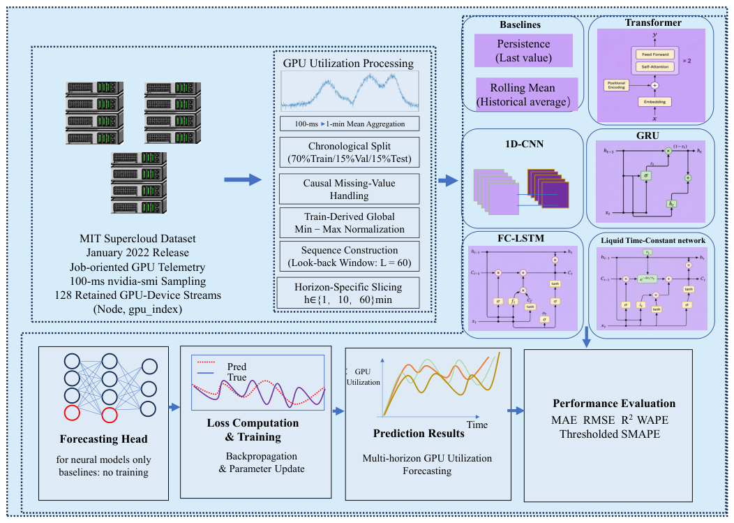
As summarized in Figure 1, the proposed framework connects GPU-device reconstruction, temporal aggregation, horizon-specific forecasting, baseline comparison, and performance evaluation.

The objective of this study is to predict future GPU utilization from historical telemetry as potential input to proactive resource management decisions. The released telemetry contains observations from multiple GPU devices, and the forecasting unit is defined as one reconstructed GPU device stream identified by (Node,gpu_index), rather than a physical compute node or a sequence formed by concatenating different devices. Let M denote the number of retained GPU devices. For GPU device m, the utilization sequence is

$${\mathcal{X}}^{\left(m\right)}=\left\{x_1^{\left(m\right)},x_2^{\left(m\right)},\dots ,x_{T_m}^{\left(m\right)}\right\},m=1,2,\dots ,M,$$

(1)

where $x_t^{\left(m\right)}\in [0,100]$ is the GPU utilization percentage at time step t, and $T_m$ is the length of the sequence for GPU device m.

Each GPU device is treated as an independent univariate time series. Sliding-window samples are generated separately from each device and are pooled only at the sample level. For a given forecast horizon, one global model is trained, with parameters shared across devices; parameters are not shared across different forecast horizons. Thus, every input–target pair originates from one GPU device, and the prediction target is GPU device-level utilization.

Given a look-back length L, the historical input available at forecast origin t is

$${\mathbf{X}}_t^{\left(m\right)}={\left[x_{t-L+1}^{\left(m\right)},x_{t-L+2}^{\left(m\right)},\dots ,x_t^{\left(m\right)}\right]}^{\top }\in {\mathbb{R}}^{L\times 1}.$$

(2)

Let

$$\mathcal{H}=\{1,10,60\}$$

(3)

denote the evaluated forecast horizons in units of the 1 min sampling interval. For $h\in \mathcal{H}$, the raw-scale target associated with forecast origin t is defined as

$$y_t^{(m,h)}=x_{t+h}^{\left(m\right)},t=L,\dots ,T_m-h.$$

(4)

Accordingly, ${\widehat{y}}_t^{(m,h)}$ denotes the prediction made at time t for GPU device m and target time $t+h$.

A direct horizon-specific strategy is adopted. A separate scalar model is trained for each h:

$${\widehat{y}}_t^{(m,h)}=f^{\left(h\right)}\left({\mathbf{X}}_t^{\left(m\right)};{\Theta }_h\right),f^{\left(h\right)}:{\mathbb{R}}^{L\times 1}\to \mathbb{R},$$

(5)

where ${\Theta }_h$ denotes the parameters of the model trained for horizon h. Predictions from shorter horizons are not recursively used as inputs to longer-horizon models.

Let $N_{m,h}$ be the number of valid training windows from GPU device m for horizon h, and let

$$N_h={\displaystyle \sum _{m=1}^M}{N}_{m,h}$$

(6)

be the corresponding number of pooled training samples. Using a pooled sample index n, the horizon-specific squared-error objective on the raw scale can be written conceptually as

$$\underset{{\Theta }_h}{min}{\displaystyle \frac{1}{N_h}}{\displaystyle \sum _{n=1}^{N_h}}{\left[y_n^{\left(h\right)}-f^{\left(h\right)}\left({\mathbf{X}}_n;{\Theta }_h\right)\right]}^2.$$

(7)

The pooled index is only notational; it does not imply temporal continuity between different GPU devices. In the actual optimization, both inputs and targets are represented on the normalized scale defined in Section 3.3.

For reporting the three independently trained forecasts at a common forecast origin t, the predictions can be collected as

$${\widehat{\mathbf{Y}}}_t^{\left(m\right)}={\left[{\widehat{y}}_t^{(m,1)},{\widehat{y}}_t^{(m,10)},{\widehat{y}}_t^{(m,60)}\right]}^{\top }.$$

(8)

This vector is a reporting convenience; it is not the output of a single multi-output network, and parameters are not shared across horizons.

3.2. Experimental Objective

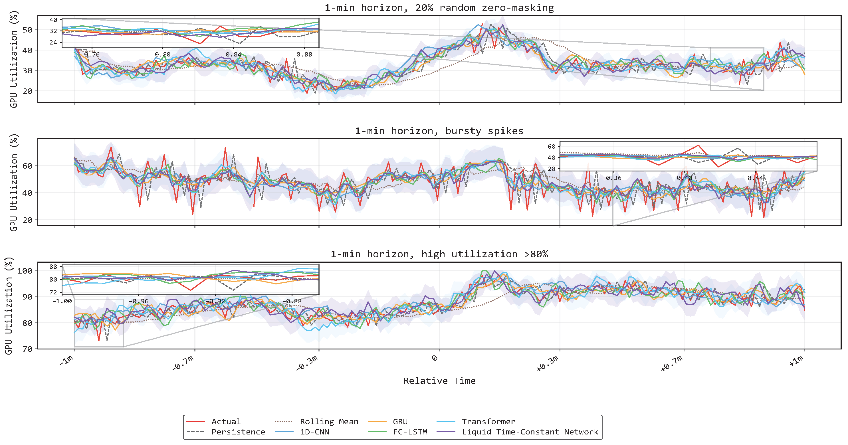
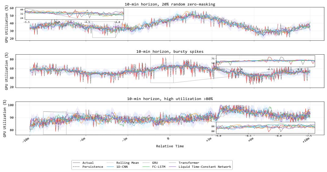
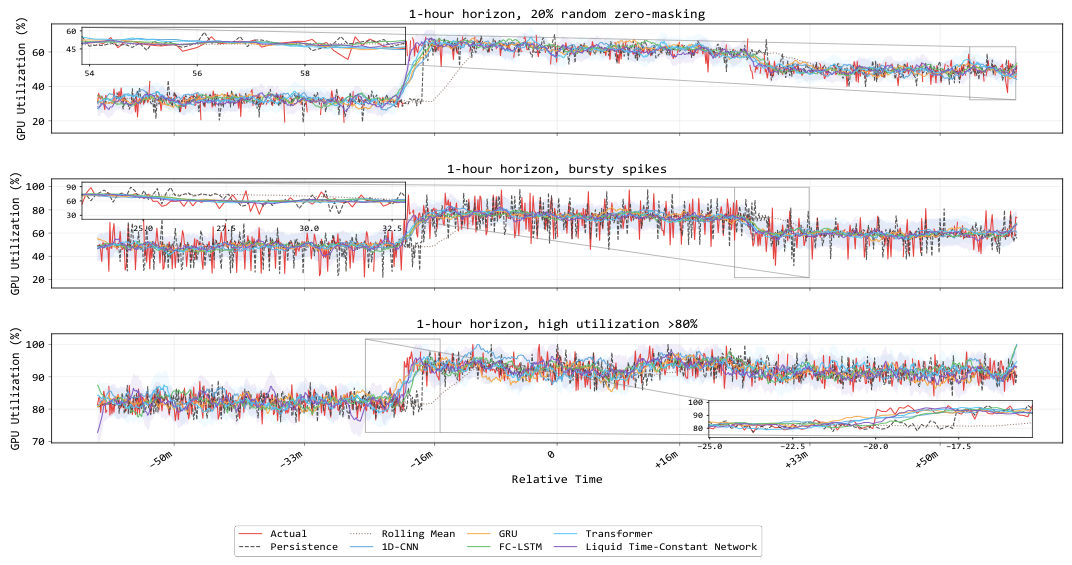
The experiment is designed around two practical questions. The first is whether the model ranking changes as the forecast is moved from the next minute to a longer planning horizon. We therefore use 1 min, 10 min, and 1 h targets, which correspond roughly to immediate scheduling, rolling allocation, and short-term capacity planning. These horizons are fixed analysis points rather than values selected after inspecting test performance.

The second question is how the models behave when the utilization trace departs from local continuity. For this reason, the overall test-set comparison is supplemented with spike events, high-load intervals, and a controlled zero-masking experiment. The same chronological split, eligible targets, preprocessing rules, GPU device-level macro-averaging, and diagnostic subsets are used for persistence, rolling mean, 1D-CNN, GRU, FC-LSTM, LTC, and Transformer so that differences in preprocessing do not enter the comparison. LTC provides the continuous-time recurrent alternative in this set; the experiments are used to determine whether its adaptive state dynamics are useful for these traces, rather than assuming that they are beneficial in advance.

A 60-sample input window is used throughout the study. At the 1 min resampling interval, this corresponds to one hour of recent history. Keeping this history length fixed makes the input context comparable across the three forecasting tasks. The value is a common experimental setting, not a claim that 60 min is the universally optimal look-back length.

3.3. Dataset and Preprocessing

The experiments use the January 2022 public release of the MIT Supercloud Dataset [11]. The release is identified by the public prefix s3://mit-supercloud-dataset/datacenter-challenge/202201/ and is described by the MIT Datacenter Challenge as the data released as of January 2022 (https://dcc.mit.edu/data/ (accessed on 11 August 2026). The release contents and directory structure were reverified on 11 August 2026. GPU telemetry is read from the gpu/ directory and linked to the Slurm accounting metadata in slurm-log.csv. No additional calendar date restriction is applied in this study: all GPU timestamps available in this release are eligible before the validity and forecasting-window filters described below. The source dataset paper reports a six-month collection window and notes that collection was ongoing [11]. Because the public release page does not publish calendar endpoints for this six-month window, unsupported start/end dates are not introduced here. Instead, the release-specific extraction procedure records the exact minimum and maximum raw and retained timestamps from the released timestamp field in a reproducibility manifest.

The released GPU telemetry is job-oriented rather than a set of preconstructed continuous machine-level series. The MIT collection procedure monitors every GPU assigned to a job with the NVIDIA nvidia-smi utility at 100 ms intervals [11]. The GPU time-series schema used in the present extraction contains the anonymized identifiers id_job and Node, together with timestamp, gpu_index, and utilization_gpu_pct. The latter is the only telemetry variable used as a forecasting input. Other released GPU measurements, such as memory utilization, memory footprint, temperature, power draw, and PCIe information, are not used by the forecasting models.

Identifier linkage follows the relationships preserved in the public release. The dataset authors added the corresponding job identifier and node name to the GPU traces because nvidia-smi itself is not scheduler-aware, and the same anonymized identifiers are used across the released files [11]. We therefore join GPU telemetry to slurm-log.csv on the anonymized id_job. The GPU Node value is checked against the node allocation represented by the scheduler nodelist whenever this field is available. Within a node, gpu_index identifies the GPU device; it is not treated as globally unique. Consequently, the forecasting-series identifier is the composite key $(\mathtt{Node},\mathtt{gpu}\_\mathtt{index})$. Scheduler fields id_array_job and id_array_task, when present, are inherited from the scheduler record matched by id_job; they are metadata and are not used as an independent second join or as the forecasting series identifier. This distinction prevents job, array task, node, and GPU device identifiers from being conflated.

The public repository reports 98,177 jobs that requested GPUs, whereas the 12,568 value used in this manuscript is a study-specific post-filtering count rather than a property of the full public dataset. To remove the ambiguity in the phrase “GPU-related tasks”, we define this quantity here as 12,568 contributing GPU jobs, i.e., distinct anonymized id_job values whose GPU observations contribute to at least one of the final retained GPU device streams. Array job and array task identifiers remain attached to the scheduler records when applicable, but they are not counted as separate forecasting devices.

For temporal reconstruction, observations belonging to the same (Node,gpu_index) key are ordered by timestamp. The raw 100 ms utilization_gpu_pct measurements are then aggregated onto a fixed 1 min grid by taking the arithmetic mean of all valid observations within each minute. If no valid observation is present in a minute, the grid point is marked as missing. Thus, 100 ms is the acquisition interval of the source GPU telemetry, whereas 1 min is the forecasting resolution used in this study; $h\in \{1,10,60\}$ therefore corresponds directly to 1-min-, 10-min-, and 1-h-ahead forecasting.

The final subset is selected in the following fixed order. First, records with an invalid id_job, Node, timestamp, gpu_index, or utilization_gpu_pct are removed and GPU records without a matching scheduler job are excluded. Second, the remaining records are reconstructed into (Node,gpu_index)-level streams and aggregated to the 1 min grid. Third, each stream is split chronologically into 70%/15%/15% training, validation, and test subsets, after which the split-local causal gap rules below are applied. Figure 2 provides a schematic overview of this chronological data partition and the associated leakage prevention protocol. The 70%/15%/15% boundaries are determined separately from the available chronology of each retained GPU device stream; no universal absolute timestamp is shared across all devices. For a resampled stream of length $T_m$, define

$$b_{m,1}=⌊0.70T_m⌋,b_{m,2}=⌊0.85T_m⌋.$$

The training subset contains indices $1,\dots ,b_{m,1}$, validation contains $b_{m,1}+1,\dots ,b_{m,2}$, and test contains $b_{m,2}+1,\dots ,T_m$. Because $T_m$ and the retained timestamp range can differ by device, the corresponding calendar-time split boundaries can also differ. All imputation, normalization eligibility checks, and window construction are then restricted to the resulting split-local data. Finally, a GPU device is retained only when it yields at least one eligible input–target window in each of the training, validation, and test subsets for all three horizons $h\in \{1,10,60\}$. A validation or test target is eligible only when its target timestamp was originally observed before imputation. Applying this pipeline gives the 128 GPU device time series and 12,568 contributing GPU jobs used in the experiments. The value 128 therefore refers to retained GPU device streams, not to 128 physical compute nodes.

The raw-to-analysis extraction and audit procedure is implemented with a release-specific reproducibility script. The procedure records the release prefix, input directories/files, raw fields, join keys, minimum and maximum raw and retained timestamps, row counts after each filtering stage, number of contributing id_job values, and number of retained $(\mathtt{Node},\mathtt{gpu}\_\mathtt{index})$ streams in an audit manifest. This keeps the release-specific time span and selection counts data-derived rather than manually inferred from file names or publication dates.

After temporal aggregation, each retained GPU device produces an independent univariate utilization sequence,

$${\mathcal{X}}^{\left(m\right)}=\left\{x_1^{\left(m\right)},x_2^{\left(m\right)},\dots ,x_{T_m}^{\left(m\right)}\right\},m=1,2,\dots ,M,$$

(9)

where $x_t^{\left(m\right)}\in [0,100]$ denotes the GPU utilization percentage of GPU device m at time step t, $T_m$ is the length of its 1 min sequence, and $M=128$ is the number of retained GPU device streams. Streams from different devices are neither concatenated nor averaged. Sliding-window samples are generated separately for each device and are pooled only at the sample level for global model training.

The main characteristics of the processed dataset are summarized in

Table 1. Reproducible specifications of the MIT Supercloud GPU utilization subset used in this study.

Item	Description
Dataset release	MIT Supercloud Dataset, January 2022 public release
Public S3 prefix	datacenter-challenge/202201/
Access date	11 August 2026
GPU directory/scheduler file	gpu//slurm-log.csv
Source collection window	6 months (ongoing), as reported by the source dataset paper
Study timespan rule	Full GPU timestamp span of the January 2022 release; no additional calendar cutoff
Raw GPU acquisition interval	100 ms using nvidia-smi
Identifier fields used	id_job, Node, gpu_index
Time/value fields used	timestamp, utilization_gpu_pct
Scheduler linkage	id_job; Node checked against nodelist
Array identifiers	id_array_job/id_array_task retained as scheduler metadata, not device keys
GPU device identifier	$(\mathtt{Node},\mathtt{gpu}\_\mathtt{index})$
GPU requesting jobs in public repository	98,177
Contributing GPU jobs after study filters	12,568 distinct id_job values
Retained forecasting streams	128 GPU device time series
Temporal aggregation	100 ms observations → 1 min mean
Forecasting variable	GPU utilization
Measurement unit	Percentage (%)
Valid range	0–100%
Resampled interval	1 min
Window generation rule	Per-device, horizon-specific, split-contained
Natural missing ratio	8.7%
Training/validation/test split	70%/15%/15%
Split boundary rule	Per-GPU-device relative chronology using $b_{m,1}=\lfloor 0.70T_m\rfloor$ and $b_{m,2}=\lfloor 0.85T_m\rfloor$; no global absolute-time cutoff
Extraction/audit procedure	Release-specific reproducibility script with an audit manifest

.

The 8.7% natural missing ratio is calculated after 1 min aggregation and before imputation. Each GPU device sequence is then divided chronologically into training, validation, and test subsets using proportions of 70%, 15%, and 15%, respectively. Missing-value processing is performed independently inside each subset, and no filling or interpolation operation is allowed to cross a split boundary. Within a subset, forward filling is applied to gaps shorter than 10 min. For gaps from 10 to 30 min, linear interpolation is permitted only for a forecasting sample whose forecast origin occurs at or after the right-hand valid endpoint used by the interpolation. If constructing a sample would require an interpolated input that depends on an observation later than the sample’s forecast origin, the sample is discarded rather than using the future observation. Segments containing gaps longer than 30 min are also excluded from sliding-window construction. This sample-wise causality constraint prevents both cross-split leakage and within-split look-ahead leakage.

For validation and test evaluation, the target timestamp must correspond to an originally observed valid GPU utilization record before imputation. A candidate sample whose target value is missing in the resampled data before imputation is excluded from metric computation. Imputation is therefore used only to recover eligible historical input values under the causal rule above and is never used to manufacture validation or test ground-truth targets.

Artificial input corruption is introduced only in the robustness evaluation by randomly replacing originally valid normalized historical inputs with zero; the forecasting targets are left unchanged. This zero-masking protocol is therefore distinct from the naturally missing records handled during preprocessing and should not be interpreted as a realistic missing-value token.

Random splitting is avoided because it would disrupt the temporal order of each utilization sequence and could produce overly optimistic forecasting results. For the m-th GPU device, the chronological split is defined as

$$\begin{array}{cc}\hfill {\mathcal{D}}_{\mathrm{train}}^{\left(m\right)}& =\left\{x_1^{\left(m\right)},\dots ,x_{\lfloor 0.70T_m\rfloor }^{\left(m\right)}\right\},\hfill \\ \hfill {\mathcal{D}}_{\mathrm{val}}^{\left(m\right)}& =\left\{x_{\lfloor 0.70T_m\rfloor +1}^{\left(m\right)},\dots ,x_{\lfloor 0.85T_m\rfloor }^{\left(m\right)}\right\},\hfill \\ \hfill {\mathcal{D}}_{\mathrm{test}}^{\left(m\right)}& =\left\{x_{\lfloor 0.85T_m\rfloor +1}^{\left(m\right)},\dots ,x_{T_m}^{\left(m\right)}\right\}.\hfill \end{array}$$

(10)

All sliding-window samples are generated independently within their corresponding subsets. Any input–target pair crossing a subset boundary is discarded, as is any window containing an imputed value whose construction would require an observation later than the window’s forecast origin.

To improve training stability, min–max normalization is applied after the chronological split. The normalization parameters are calculated exclusively from the training data:

$$z_t^{\left(m\right)}={\displaystyle \frac{x_t^{\left(m\right)}-X_{min}^{\mathrm{train}}}{X_{max}^{\mathrm{train}}-X_{min}^{\mathrm{train}}}},$$

(11)

where $X_{min}^{\mathrm{train}}$ and $X_{max}^{\mathrm{train}}$ are computed globally from all valid training observations pooled across the 128 retained GPU devices. A single pair of training-derived normalization parameters is therefore shared by all GPU devices and all forecast horizons. The same parameters are subsequently applied unchanged to the validation and test sets to prevent information leakage.

During model training, the loss is computed on the normalized scale. Before final evaluation, each predicted value is transformed back to the original utilization scale using

$${\widehat{y}}_t^{(m,h)}={\widehat{z}}_t^{(m,h)}\left(X_{max}^{\mathrm{train}}-X_{min}^{\mathrm{train}}\right)+X_{min}^{\mathrm{train}},$$

(12)

where ${\widehat{z}}_t^{(m,h)}$ is the normalized horizon-specific model output and ${\widehat{y}}_t^{(m,h)}$ is the corresponding prediction on the original 0–100% GPU utilization scale. Predictions are not clipped to the physical 0–100% range before metric computation; this avoids artificially improving the reported errors through post-processing. Figures may restrict the displayed vertical axis to the physical utilization range, but all quantitative metrics use the unclipped inverse-normalized predictions. Consequently, the MAE and RMSE are reported in percentage points, while relative error metrics are reported as percentages.

3.4. Multi-Horizon Forecasting Formulation

Based on the chronologically partitioned and normalized 1 min GPU utilization sequences, sliding-window samples are generated independently within the training, validation, and test subsets of each GPU device. For GPU device m and time step t, the model input of length L is

$${\mathbf{Z}}_t^{\left(m\right)}={\left[z_{t-L+1}^{\left(m\right)},z_{t-L+2}^{\left(m\right)},\dots ,z_t^{\left(m\right)}\right]}^{\top }\in {\mathbb{R}}^{L\times 1},$$

(13)

where $z_t^{\left(m\right)}$ is the normalized utilization defined in Equation (11). Each window contains observations from only one GPU device and one data subset. Windows whose inputs or prediction targets would cross the training, validation, or test boundaries are discarded.

For a forecasting horizon $h\in \mathcal{H}$, the normalized target and its raw-scale counterpart are written consistently as

$$z_t^{(m,h)}=z_{t+h}^{\left(m\right)},y_t^{(m,h)}=x_{t+h}^{\left(m\right)}.$$

(14)

Thus, the subscript t denotes the forecast origin, and the superscript $(m,h)$ identifies the GPU device and forecast horizon.

This study adopts a direct horizon-specific forecasting strategy. Instead of using one multi-output model for all evaluated lead times, an independent scalar forecasting model is trained for each horizon. For horizon h, the normalized prediction is

$${\widehat{z}}_t^{(m,h)}=f^{\left(h\right)}\left({\mathbf{Z}}_t^{\left(m\right)};{\Theta }_h\right),f^{\left(h\right)}:{\mathbb{R}}^{L\times 1}\to \mathbb{R}.$$

(15)

For evaluation, ${\widehat{z}}_t^{(m,h)}$ is transformed back to the original scale using Equation (12), yielding ${\widehat{y}}_t^{(m,h)}$.

We use three lead times, $h\in \{1,10,60\}$, corresponding to 1 min, 10 min, and 1 h forecasts. These horizons cover three operational scales that are relevant to GPU management: immediate reaction, short rolling allocation, and hour-ahead planning. A separate neural model is trained for each lead time, so longer-horizon predictions are not produced recursively from shorter-horizon forecasts. The two deterministic baselines are evaluated separately at the same three lead times.

The look-back window is fixed at $L=60$, giving every neural model and the rolling mean baseline one hour of recent history at the 1 min sampling rate. This was used as a practical compromise: it includes short bursts as well as slower level changes visible in the traces, without introducing a separate look-back search for every architecture and horizon. The same 60-step context is therefore retained across the comparison. The rolling mean baseline uses this full 60-step history, whereas persistence uses the most recent value at the forecast origin.

3.5. Forecasting Models

To evaluate different sequence-modeling mechanisms for GPU utilization forecasting, five neural forecasting models are compared under the same data and evaluation protocol: 1D-CNN, GRU, FC-LSTM, Liquid Time-Constant Network (LTC), and Transformer. Two deterministic baselines, persistence and rolling mean, are added to provide simple reference forecasts. For readability, the GPU device superscript $\left(m\right)$ is suppressed in the model-specific equations below. For all models, the input is the normalized historical window

$${\mathbf{Z}}_t\in {\mathbb{R}}^{L\times 1},$$

(16)

where L is the look-back window length, and the single channel corresponds to normalized GPU utilization. Under the direct horizon-specific formulation, each model outputs one normalized scalar prediction

$${\widehat{z}}_t^{\left(h\right)}\in \mathbb{R}.$$

(17)

For each horizon $h\in \{1,10,60\}$, an independent neural model is trained; predictions are inverse-normalized before evaluation. The two baselines are deterministic and require no training.

3.5.1. Baseline Models

The two baselines use the same GPU device-specific historical windows, chronological split, eligible forecast targets, and evaluation subsets as the neural models. They have no trainable parameters and therefore do not use the optimization procedure described in Section 3.6.

For persistence, the most recent normalized utilization value is carried forward to the target horizon:

$${\widehat{z}}_{t,\mathrm{pers}}^{\left(h\right)}=z_t,h\in \{1,10,60\}.$$

(18)

This baseline is expected to be competitive when utilization is locally stable, but it cannot anticipate a change that occurs after the forecast origin.

The rolling mean baseline uses the same 60-step history as the neural models:

$${\widehat{z}}_{t,\mathrm{roll}}^{\left(h\right)}={\displaystyle \frac{1}{L}}{\displaystyle \sum _{j=0}^{L-1}}{z}_{t-j},L=60,h\in \{1,10,60\}.$$

(19)

The averaging length is fixed at $L=60$ before test evaluation rather than selected from test performance. Both baseline predictions are inverse-normalized and scored using the same GPU device-level macro-averaging procedure as the neural models.

3.5.2. 1D-CNN

The 1D-CNN model is used to capture local temporal patterns in GPU utilization traces, such as abrupt spikes, short-term bursts, and transient drops. Given the input window ${\mathbf{Z}}_t\in {\mathbb{R}}^{L\times 1}$, one-dimensional convolutional filters slide along the temporal dimension to extract local features from neighboring time steps.

The 1D-CNN architecture consists of stacked one-dimensional convolutional layers followed by nonlinear activation functions. Instead of flattening the entire feature map, global average pooling is applied along the temporal dimension to obtain a compact representation of the extracted temporal features. This design reduces the number of parameters in the forecasting head relative to flattening the full feature map and provides a compact temporal representation [27]. The pooled representation is then passed to a fully connected layer to produce the horizon-specific normalized scalar prediction:

$${\widehat{z}}_t^{\left(h\right)}=f_{\mathrm{CNN}}^{\left(h\right)}({\mathbf{Z}}_t;{\Theta }_h).$$

(20)

This architecture emphasizes the local temporal structure and permits convolutional feature extraction across the input window. Since the receptive field is determined by the convolutional stack, its relative effectiveness for longer-range dependencies is assessed empirically rather than assumed from the architecture.

3.5.3. GRU

GRU is selected as a lightweight recurrent architecture for sequence forecasting. It uses update and reset gates to regulate hidden-state transitions and control how much historical information is retained or refreshed [26]. Compared with LSTM, GRU has a more compact gating structure.

For the input window ${\mathbf{Z}}_t\in {\mathbb{R}}^{L\times 1}$, the GRU encoder processes the sequence step by step and produces a final hidden representation. This representation is then fed into a fully connected forecasting head to generate the horizon-specific normalized scalar output:

$${\widehat{z}}_t^{\left(h\right)}=f_{\mathrm{GRU}}^{\left(h\right)}({\mathbf{Z}}_t;{\Theta }_h).$$

(21)

In this comparison, GRU provides a discrete-time recurrent baseline with a compact gating structure. Its behavior under abrupt workload changes is evaluated empirically rather than inferred from the recurrence mechanism alone.

3.5.4. FC-LSTM

FC-LSTM combines an LSTM temporal encoder with fully connected output layers [9]. The LSTM component captures temporal dependencies through input, forget, and output gates, while the fully connected layers map the final hidden representation to a normalized scalar forecast. The implementation uses the capacity-controlled architecture reported in Table 3, so the primary cross-model comparison is conducted under an approximately common trainable parameter budget.

Given the input sequence ${\mathbf{Z}}_t\in {\mathbb{R}}^{L\times 1}$, the LSTM encoder updates its hidden state along the temporal dimension. The final hidden state is used as the temporal representation of the historical window and is passed to a fully connected forecasting head that outputs the normalized horizon-specific prediction:

$${\widehat{z}}_t^{\left(h\right)}=f_{\mathrm{LSTM}}^{\left(h\right)}({\mathbf{Z}}_t;{\Theta }_h).$$

(22)

Compared with GRU, LSTM maintains a separate cell state in addition to the hidden state. FC-LSTM is therefore included as a recurrent architecture with a different memory structure; any performance advantage is assessed from the experimental results rather than assumed from the architecture.

3.5.5. Liquid Time-Constant Network

Liquid Time-Constant Network (LTC) is introduced to evaluate whether continuous-time, input-dependent neural dynamics are suitable for nonstationary GPU utilization forecasting. Different from LSTM and GRU, which update hidden states at discrete time steps, LTC models hidden-state evolution using ordinary differential equations. Therefore, LTC is not a variant of LSTM but a continuous-time recurrent neural network with a different mathematical foundation.

The LTC used in this study is a custom PyTorch implementation of the standard LTC dynamical form [10]. The implementation uses PyTorch 1.12.1 and torchdiffeq 0.2.3 [37] for numerical ODE integration. It does not use the ncps LTC layer, so the equations and solver settings below correspond directly to the implementation used in the experiments.

For an LTC layer, the hidden state $\mathbf{h}\left(s\right)\in {\mathbb{R}}^{d_h}$ evolves over continuous time s. For hidden unit j,

$${\displaystyle \frac{d{h}_j\left(s\right)}{ds}}=-\left[{\displaystyle \frac{1}{{\tau }_j}}+f_j\left(\mathbf{h}\left(s\right),x\left(s\right)\right)\right]h_j\left(s\right)+f_j\left(\mathbf{h}\left(s\right),x\left(s\right)\right)A_j,$$

(23)

where $d_h=128$, $A_j$ is a learnable equilibrium parameter, and ${\tau }_j>0$ is the base time constant.

The nonlinear gating vector $\mathbf{f}={[f_1,\dots ,f_{d_h}]}^{\top }$ is parameterized explicitly as

$$\mathbf{f}\left(\mathbf{h}\left(s\right),x\left(s\right)\right)=\sigma \left({\mathbf{W}}_h\mathbf{h}\left(s\right)+{\mathbf{W}}_{x}x\left(s\right)+{\mathbf{b}}_f\right),$$

(24)

where ${\mathbf{W}}_h\in {\mathbb{R}}^{128\times 128}$, ${\mathbf{W}}_x\in {\mathbb{R}}^{128\times 1}$, ${\mathbf{b}}_f\in {\mathbb{R}}^{128}$, and $\sigma \left(a\right)=1/(1+e^{-a})$ is the element-wise logistic sigmoid. The positive base time constants are parameterized by

$$\mathit{\tau }=softplus\left({\mathit{\rho }}_{\tau }\right)+{10}^{-3},{\mathit{\rho }}_{\tau }\in {\mathbb{R}}^{128},$$

(25)

while $\mathbf{A}\in {\mathbb{R}}^{128}$ is learned directly. Thus, the complete trainable parameter set of the LTC dynamics is $\{{\mathbf{W}}_h,{\mathbf{W}}_x,{\mathbf{b}}_f,{\mathit{\rho }}_{\tau },\mathbf{A}\}$.

Equation (23) defines the effective time constant

$${\tau }_{\mathrm{sys},j}\left(s\right)={\displaystyle \frac{{\tau }_j}{1+{\tau }_j{f}_j(\mathbf{h}\left(s\right),x\left(s\right))}}.$$

(26)

The normalized 1 min observations are supplied to the continuous-time dynamics using zero-order hold interpolation:

$$x\left(s\right)=z_{t-L+1+k},s\in [k,k+1),k=0,\dots ,L-1.$$

(27)

One ODE time unit corresponds to one minute. Starting from the non-trainable initial state $\mathbf{h}\left(0\right)=\mathbf{0}$, the encoder performs 60 consecutive one-minute integrations, so a complete $L=60$ window corresponds to $s\in [0,60]$. No future observation is used to interpolate the input within an interval.

Each one-minute transition is solved with torchdiffeq.odeint using method=’dopri5’, relative tolerance ${10}^{-4}$, and absolute tolerance ${10}^{-6}$. The solver uses adaptive internal step sizes; no fixed step_size is supplied and the library’s default adaptive-step controller is retained. Standard odeint, rather than odeint_adjoint, is used.

The final hidden state $\mathbf{h}\left(60\right)$ is passed to a horizon-specific forecasting head with widths $128\to 192\to 64\to 16\to 1$. The three hidden fully connected layers use ReLU activation and dropout $p=0.2$; the scalar output layer is linear. The resulting forecast is

$${\widehat{z}}_t^{\left(h\right)}={\mathbf{W}}_4\varphi \left({\mathbf{W}}_3\varphi \left({\mathbf{W}}_2\varphi \left({\mathbf{W}}_1\mathbf{h}\left(60\right)+{\mathbf{b}}_1\right)+{\mathbf{b}}_2\right)+{\mathbf{b}}_3\right)+b_4,$$

(28)

where $\varphi (·)=ReLU(·)$. Dropout is omitted from Equation (28) for notational clarity and is active only during training.

The exact LTC trainable parameter count is 55,073. The dynamical part contains 16,896 parameters: $128\times 128$ in ${\mathbf{W}}_h$, $128\times 1$ in ${\mathbf{W}}_x$, 128 in ${\mathbf{b}}_f$, 128 in ${\mathit{\rho }}_{\tau }$, and 128 in $\mathbf{A}$. The forecasting head contains 38,177 parameters, giving 16,896 + 38,177 = 55,073 trainable parameters in total. The zero initial state and the integration-time grid are non-trainable.

Because dopri5 is adaptive, the number of right-hand-side function evaluations (NFE) is input-dependent rather than a fixed model hyperparameter. Every call to the right-hand side of Equation (23) increments a forward NFE counter. The NFE of one 60-sample input window is the sum of these calls over the 60 one-minute integrations, including evaluations from rejected adaptive steps. Since standard odeint is used, there is no separate backward ODE re-solve; NFE therefore refers to forward right-hand-side evaluations. The reproducibility implementation logs the per-window NFE and its mean, standard deviation, minimum, and maximum together with the LTC runtime statistics. Across the eligible 1 h test windows, the adaptive solver required $1316\pm 73$ forward right-hand-side evaluations per 60-step input window (mean ± standard deviation), with an observed range of 1188–1512 evaluations. Because the solver is adaptive, NFE varies with the input window and is therefore reported as a distribution rather than a fixed architectural constant.

This formulation provides LTC with a state- and input-dependent dynamical timescale. Its relevance to abrupt spikes, regime transitions, and nonstationary workload patterns is evaluated empirically rather than treated as an a priori performance guarantee [10].

3.5.6. Transformer

The Transformer model is included to evaluate the effectiveness of self-attention for GPU utilization forecasting [28]. Unlike recurrent models, Transformer does not process the input sequence strictly step by step. Instead, its self-attention mechanism directly computes dependencies among different time steps within the input window, allowing the model to capture temporal relationships over the entire look-back range.

For the input window ${\mathbf{Z}}_t\in {\mathbb{R}}^{L\times 1}$, positional encoding is added to preserve temporal order information. The encoded sequence is then processed by Transformer encoder layers. The resulting temporal representation is aggregated and passed to a fully connected forecasting head to produce the horizon-specific normalized scalar prediction:

$${\widehat{z}}_t^{\left(h\right)}=f_{\mathrm{Trans}}^{\left(h\right)}({\mathbf{Z}}_t;{\Theta }_h).$$

(29)

The Transformer provides a non-recurrent self-attention architecture that can represent dependencies across the full look-back window. Its relative performance can depend on the data regime, horizon, and model configuration; therefore, it is evaluated under the same protocol as the recurrent and convolutional alternatives without assuming an a priori ranking.

3.6. Training Configuration

The same data split, input history, target definition, and optimization loss are used across the five neural model families, where these choices are architecture-independent. For each $h\in \{1,10,60\}$, a separate scalar-output neural model is trained, so the three horizons correspond to independent optimization runs rather than a single multi-output network. Persistence and rolling mean require no training or parameter optimization. Architecture-specific choices—for example, the attention dimension or ODE integration—remain model-dependent.

For horizon h, the mean squared error on the normalized scale is used as the training loss:

$${\mathcal{L}}^{\left(h\right)}={\displaystyle \frac{1}{N_{\mathrm{train}}^{\left(h\right)}}}{\displaystyle \sum _{i=1}^{N_{\mathrm{train}}^{\left(h\right)}}}{\left({\widehat{z}}_i^{\left(h\right)}-z_i^{\left(h\right)}\right)}^2,$$

(30)

where $N_{\mathrm{train}}^{\left(h\right)}$ is the number of pooled training samples available for horizon h, $z_i^{\left(h\right)}$ is the normalized h-step-ahead target, and ${\widehat{z}}_i^{\left(h\right)}$ is the corresponding normalized prediction. Final evaluation metrics are calculated after inverse normalization on the original 0–$100\%$ utilization scale.

The weighting implicit in the training objective differs from the GPU device macro-averaging used for the reported evaluation metrics. In the implementation, all eligible training windows from the retained GPU devices are placed in one pooled training set, the pooled list is shuffled at the start of each epoch, and ordinary mini-batches of size 128 are drawn from this shuffled list. No GPU device-balanced sampler and no inverse-frequency device weighting are applied. Therefore, if $N_{m,h}^{\mathrm{train}}$ denotes the number of eligible training windows contributed by GPU device m at horizon h, the effective training weight of this device is

$$w_{m,h}^{\mathrm{train}}={\displaystyle \frac{N_{m,h}^{\mathrm{train}}}{{\sum }_{j=1}^M{N}_{j,h}^{\mathrm{train}}}}.$$

(31)

Equivalently, the pooled objective can be written as

$${\mathcal{L}}^{\left(h\right)}={\displaystyle \sum _{m=1}^M}{w}_{m,h}^{\mathrm{train}}\left[{\displaystyle \frac{1}{N_{m,h}^{\mathrm{train}}}}{\displaystyle \sum _{i=1}^{N_{m,h}^{\mathrm{train}}}}{\left({\widehat{z}}_{m,i}^{\left(h\right)}-z_{m,i}^{\left(h\right)}\right)}^2\right].$$

(32)

Thus, a GPU device with more valid training windows has a proportionally greater influence on parameter optimization. This window-weighted training objective is now stated explicitly and is distinguished from evaluation, where each eligible GPU device receives equal weight through the macro-averaging definitions in Equations (34) and (45).

The observed distribution of valid training-window counts across the 128 retained GPU devices is summarized in

Table 2. Distribution of eligible training window counts across the 128 retained GPU devices after chronological splitting, causal gap handling, and horizon-specific target eligibility filtering.

Horizon	Min	Q1	Median	Mean	SD	Q3	Max	Total
1 min	16,000	33,442	45,445	46,791	18,391	57,713	90,000	5,989,210
10 min	15,982	33,427	45,420	46,770	18,391	57,703	89,986	5,986,587
1 h	15,868	33,338	45,329	46,688	18,394	57,565	89,903	5,976,102

. The distribution confirms that the devices contribute unequal numbers of windows to the pooled objective: the median retained device contributes roughly 45,000 training windows, whereas the largest contributes roughly 90,000.

Optimization uses Adam [38]. Validation data are used only to decide when to stop training and which checkpoint to retain; the test set is not used for model selection. The settings in

Table 3. Primary neural model configurations after approximate capacity control.

Model	Configuration	Trainable Parameters
1D-CNN	Conv1D filters: 48, 104, 128; kernel size: 3; GAP	55,465
GRU	1 recurrent layer; 134 hidden units	55,209
FC-LSTM	1 LSTM layer; 106 hidden units; FC: 64, 32	55,177
LTC	128 hidden units; FC: 192, 64, 16	55,073
Transformer	$d_{\mathrm{model}}=56$; 4 heads; $d_{\mathrm{ff}}=128$; 2 encoder layers	55,193

Note: Persistence and rolling mean have no trainable parameters and are not included in the capacity-matching procedure. Counts include trainable biases and output layers; sinusoidal positional encoding is non-trainable. Widths were selected as the nearest usable configurations around the LTC reference scale, subject to the structural constraints of each architecture.

and 

Table 4. Training configuration.

Parameter	Setting
Dataset	MIT Supercloud GPU utilization data
Sampling interval	1 min
Input window length	$L=60$
Forecasting horizons	$h=1,10,60$
Forecasting targets	1 min, 10 min, and 1 h ahead
Data split	Chronological 70%/15%/15%
Input dimension	$L\times 1$
Output dimension	One scalar per separately trained horizon model
Optimizer	Adam
Learning rate	$1\times {10}^{-3}$
Loss function	Mean squared error
Batch size	128
Training window sampler	Uniform shuffle over pooled eligible windows; no GPU device balancing
Maximum epochs	200
Early stopping criterion	Validation loss
Early stopping patience	20 epochs
Dropout rate	0.2
Weight decay	$1\times {10}^{-5}$
Normalization scope	Global min–max from pooled training observations
Prediction clipping	None before metric computation
Hyperparameter policy	Fixed prespecified configurations; no test-set tuning
Capacity reference scale	LTC-128 configuration, approximately 55,000 trainable parameters
Capacity selection	Nearest feasible architecture-specific width around the reference scale
Random seeds	2021, 2022, 2023, 2024, 2025
Number of repeated runs	5
Neural models	1D-CNN, GRU, FC-LSTM, LTC, Transformer
Baselines	Persistence; rolling mean ($L=60$); no training
LTC implementation	Custom PyTorch implementation; torchdiffeq 0.2.3
LTC hidden width	128
LTC gating activation	Logistic sigmoid
LTC time constants	$softplus\left({\rho }_{\tau }\right)+{10}^{-3}$
LTC input interpolation	Zero-order hold between 1 min observations
LTC ODE interval	$\Delta s=1$ per minute; 60 intervals per input window
LTC initial state	$\mathbf{h}\left(0\right)=\mathbf{0}$, non-trainable
LTC ODE solver	dopri5 adaptive-step Runge–Kutta
LTC relative/absolute tolerance	${10}^{-4}$/${10}^{-6}$
LTC step control	Adaptive; no fixed step_size; library defaults
LTC forecasting head	128–192–64–16–1; ReLU hidden layers; linear output
LTC exact trainable parameters	55,073
LTC forward NFE	$1316\pm 73$ per 60-step window; range 1188–1512

are fixed before the final evaluation rather than obtained from an exhaustive search. The input length, chronological split, normalization, loss, optimizer, batch size, and evaluation metrics are shared across the five neural model families. The baselines use the same split, processed histories, eligible targets, and evaluation metrics, but no loss, optimizer, batch size, early stopping, or random seed repetition.

Model capacity is controlled by using the 128-unit LTC configuration (55,073 trainable parameters) as a reference scale, rather than by imposing an exact parameter equality constraint. For each of the other architectures, we selected the nearest practical width that preserved its normal structural requirements. This matters most for the Transformer, whose model dimension must be divisible by the number of attention heads, and for the CNN, whose channel counts change in discrete steps. The final counts lie close together, but this closeness is a consequence of choosing the nearest feasible configurations and not a separately optimized $\pm 1\%$ target. The purpose is simply to remove the previous order-of-magnitude capacity difference before comparing the model families.

The resulting parameter counts range only from 55,073 to 55,465, but the comparison should still be regarded as capacity-controlled rather than parameter-identical. The parameter count is only one aspect of model complexity: the FLOPs, memory traffic, recurrent execution, self-attention, and adaptive ODE integration remain different. These differences are retained because removing them would also remove some aspects that distinguish the architectures.

The capacity-controlled 1D-CNN consists of three stacked one-dimensional convolutional layers with 48, 104, and 128 filters, respectively. Each convolutional layer uses a kernel size of 3 and ReLU activation. The extracted temporal feature maps are aggregated using global average pooling rather than flattening, and the pooled representation is mapped to a scalar forecast.

The capacity-controlled GRU uses one recurrent layer with 134 hidden units, followed by a scalar output layer. The capacity-controlled FC-LSTM uses one LSTM layer with 106 hidden units, followed by fully connected layers with 64 and 32 units and the final scalar output. The capacity-controlled Transformer uses sinusoidal positional encoding, 4 attention heads, $d_{\mathrm{model}}=56$, $d_{\mathrm{ff}}=128$, and 2 encoder layers. The LTC model uses 128 hidden units with the gating function in Equation (24), followed by fully connected layers of widths 192, 64, and 16 and a linear scalar output. Its exact trainable parameter count is 55,073. ODE integration uses torchdiffeq 0.2.3 with adaptive dopri5, relative tolerance ${10}^{-4}$, and absolute tolerance ${10}^{-6}$.

The detailed training configuration is shown in Table 4.

Once the model configurations were fixed, each neural model–horizon pair was rerun with five seeds (2021–2025). Neural training remained stochastic because of initialization, minibatch order, and dropout, so the repeated runs are used to report the spread of the primary metrics rather than relying on a single favorable run. The chronological split itself is unchanged across seeds. Because persistence and rolling mean are deterministic, each baseline is evaluated once per horizon on the same eligible test targets.

The 30-percentage-point spike threshold and the 80% high-load threshold are operational diagnostic definitions rather than training hyperparameters. To examine whether the diagnostic conclusions are tied to these exact values, we perform a local sensitivity check using neighboring spike cutoffs of 20, 30, and 40 percentage points and high-load cutoffs of 70%, 80%, and 90%. Model fitting, normalization, the chronological split, and the overall test metrics are unchanged; only the subset definition is recomputed.

The sensitivity analysis shows that stricter thresholds reduce the number of eligible events/targets and increase the absolute error, while the principal RMSE ordering remains unchanged across the neighboring cutoffs. In particular, LTC remains the lowest-RMSE neural model in all three spike threshold settings and all three high-load settings. This supports the interpretation of 30 percentage points and 80% as convenient diagnostic operating points rather than uniquely optimized values.

The fixed diagnostic and robustness parameters are summarized in

Table 5. Fixed diagnostic and robustness parameters used in the evaluation.

Parameter	Setting
Robustness forecast horizon	60 steps (1 h)
Random zero-masking ratio	20% of valid historical input positions
Zero-masking random seeds	2021, 2022, 2023, 2024, 2025
Robustness retraining	None; trained checkpoints evaluated directly
Spike detection threshold	30-percentage-point absolute change
Spike response error band	15 percentage points
Required consecutive in-band points	2
Spike response evaluation window	10 min
Unresolved spike delay	Capped at 10 min
High-load threshold	Ground truth utilization $>80\%$
Baseline diagnostic subsets	Identical target indices and masking realization as the compared neural models

.

The spike-threshold sensitivity results are reported in

Table 6. Sensitivity of 1 min spike RMSE and response delay to the spike detection threshold.

		Spike RMSE					Response Delay (min)
Threshold	Events	1D-CNN	GRU	FC-LSTM	LTC	Transformer	1D-CNN	GRU	FC-LSTM	LTC	Transformer
20 pp	1842	7.92	7.51	7.26	6.95	7.44	2.3	1.9	1.7	1.5	2.5
30 pp	1216	8.74	8.19	7.88	7.43	8.05	2.6	2.1	1.9	1.6	2.8
40 pp	731	9.58	8.94	8.61	8.02	8.81	3.0	2.5	2.2	1.9	3.2

Note: Bold values indicate the best (lowest) value among the five neural models for each threshold.

.

The high-load threshold sensitivity results are reported in

Table 7. Sensitivity of 1 h high-load RMSE to the utilization cutoff.

High-Load Cutoff	Eligible Targets	1D-CNN	GRU	FC-LSTM	LTC	Transformer
70%	168,420	14.82	13.51	12.74	12.30	13.14
80%	104,736	15.21	13.87	13.09	12.64	13.46
90%	46,918	16.08	14.62	13.91	13.36	14.21

Note: Bold values indicate the lowest RMSE among the five neural models for each utilization cutoff.

.

The computational environment is summarized in

Table 8. Experimental environment and observed runtime ranges.

Item	Setting
CPU	Intel Xeon Gold 6248R @ 3.00 GHz
GPU	NVIDIA Tesla V100 32 GB
RAM	256 GB
Operating system	Ubuntu 20.04 LTS
Python version	3.9.12
Deep learning framework	PyTorch 1.12.1
ODE integration library	torchdiffeq 0.2.3
CUDA version	11.6
Training time	0.5–3.5 h, depending on model complexity
Inference latency	0.5–2.0 ms per window

.

Training time is measured as the total wall-clock time from the beginning of training until early stopping. Inference latency is measured as the average prediction time per input window on the test set. These measurements are reported to evaluate not only the forecasting accuracy but also practical deployability in near-real-time GPU utilization prediction.

The approximately 55,000-parameter design controls the trainable model size only and is not a claim of equal computational cost. Across the measured runs on the common V100 environment, the total training time falls within the 0.5–3.5 h range and the average single-window inference latency within the 0.5–2.0 ms range reported in Table 8. The observed inference range is well below the 1 min telemetry interval, so the five primary neural architectures satisfy the timing requirement of the present forecasting setup. Their deployment characteristics nevertheless differ: 1D-CNN and Transformer expose greater within-window parallelism; GRU and FC-LSTM require sequential recurrent updates; and LTC additionally incurs adaptive ODE function evaluations. Parameter matching is therefore interpreted as capacity control rather than compute matching.

Table 9. Model-specific deployment profile measured on the common NVIDIA Tesla V100 environment.

Model	Parameters	Training Time (h)	Inference (ms/Window)	Peak GPU Memory (GB)
1D-CNN	55,465	$0.62\pm 0.04$	$0.54\pm 0.03$	0.48
GRU	55,209	$1.08\pm 0.06$	$0.91\pm 0.05$	0.62
FC-LSTM	55,177	$1.34\pm 0.08$	$1.07\pm 0.06$	0.70
LTC	55,073	$3.31\pm 0.14$	$1.87\pm 0.09$	1.12
Transformer	55,193	$0.96\pm 0.05$	$0.73\pm 0.04$	0.86

Note: Training time is mean ± standard deviation across five runs for the 1 h configuration. Inference latency is the mean per single input window after warm-up. Peak GPU memory is the maximum allocated GPU memory observed during inference.

reports the measured model-specific deployment profile on the common V100 environment. LTC has the largest training and inference cost because of adaptive ODE evaluation, recurrent models are intermediate, and 1D-CNN and Transformer benefit from greater within-window parallelism. For LTC, the ODE right-hand-side call counter is reset for each input window and the forward NFE is logged together with the inference time measurements.

To assess whether the principal numerical differences are consistent across GPU devices, the analysis uses the GPU device as the paired statistical unit. For each comparison, both methods are evaluated on the same eligible targets for each of the 128 retained GPU device streams, and the resulting device-level error values are paired. A two-sided Wilcoxon signed-rank test is used because normality of the paired differences is not assumed. Holm correction is applied within the six prespecified headline comparisons in

Table 10. Paired GPU device-level significance results for the six prespecified headline comparisons. Two-sided Wilcoxon signed-rank tests use the 128 retained GPU device streams as paired units, with Holm correction for multiple comparisons.

Horizon	Metric	Method A	Method B	Median Paired $\Delta$	Holm-Adjusted p	Interpretation
1 min	MAE	FC-LSTM	Persistence	−0.31 pp	0.0048	Supported difference
1 min	MAE	FC-LSTM	GRU	−0.14 pp	0.054	Not significant after correction
10 min	RMSE	LTC	Rolling Mean	−0.88 pp	<0.001	Supported difference
10 min	RMSE	LTC	Transformer	−0.24 pp	0.082	Not significant after correction
1 h	RMSE	LTC	Rolling Mean	−1.73 pp	<0.001	Supported difference
1 h	RMSE	LTC	FC-LSTM	−0.27 pp	0.164	Not significant

Note: $\Delta =$ Method A minus Method B, so negative values favor Method A for MAE/RMSE. The paired results support the improvements over simple baselines in the prespecified headline comparisons, whereas the smaller differences among the strongest neural models are not statistically established after Holm correction.

. The five training seeds continue to quantify training repeatability and are not treated as 640 independent observations.

For the primary overall forecasting comparison, each neural model–horizon configuration is trained with five random seeds (2021–2025). For each run, every evaluation metric is computed separately for each eligible GPU device and then macro-averaged according to Section 3.7.

Table 11. Overall forecasting performance across three prediction horizons. Each metric is first computed per GPU device and then macro-averaged; baseline entries are deterministic point estimates, whereas neural model entries are mean ± standard deviation over five training runs.

Horizon	Model	MAE ↓	RMSE ↓	WAPE ↓	${\mathbf{SMAPE}}_{\mathit{\eta }}$ ↓	$R^2$ ↑
1 min	Persistence	3.92	5.11	16.78	15.92	0.897
1 min	Rolling Mean	4.18	5.42	17.86	16.95	0.884
1 min	1D-CNN	$3.88\pm 0.18$	$5.06\pm 0.26$	$16.42\pm 1.10$	$15.64\pm 1.00$	$0.901\pm 0.009$
1 min	GRU	$3.71\pm 0.16$	$4.71\pm 0.23$	$15.98\pm 1.00$	$15.11\pm 0.90$	$0.912\pm 0.009$
1 min	FC-LSTM	$\mathbf{3.55}\pm \mathbf{0.15}$	$\mathbf{4.39}\pm \mathbf{0.22}$	$\mathbf{14.85}\pm \mathbf{0.82}$	$\mathbf{14.05}\pm \mathbf{0.82}$	$\mathbf{0.927}\pm \mathbf{0.006}$
1 min	LTC	$3.67\pm 0.17$	$4.64\pm 0.23$	$15.32\pm 0.92$	$14.63\pm 0.87$	$0.914\pm 0.008$
1 min	Transformer	$3.80\pm 0.18$	$4.82\pm 0.25$	$15.87\pm 1.02$	$15.04\pm 0.93$	$0.906\pm 0.009$
10 min	Persistence	6.21	8.05	21.43	20.36	0.741
10 min	Rolling Mean	6.08	7.82	20.88	19.97	0.756
10 min	1D-CNN	$6.39\pm 0.30$	$8.03\pm 0.42$	$21.95\pm 1.50$	$20.80\pm 1.30$	$0.742\pm 0.015$
10 min	GRU	$5.92\pm 0.26$	$7.41\pm 0.37$	$20.50\pm 1.30$	$19.55\pm 1.20$	$0.779\pm 0.014$
10 min	FC-LSTM	$\mathbf{5.48}\pm \mathbf{0.24}$	$7.28\pm 0.35$	$19.62\pm 1.15$	$18.82\pm 1.05$	$0.788\pm 0.012$
10 min	LTC	$5.73\pm 0.25$	$\mathbf{6.87}\pm \mathbf{0.33}$	$18.98\pm 1.10$	$18.15\pm 1.02$	$\mathbf{0.812}\pm \mathbf{0.011}$
10 min	Transformer	$5.81\pm 0.27$	$7.15\pm 0.36$	$\mathbf{18.55}\pm \mathbf{1.08}$	$\mathbf{18.03}\pm \mathbf{1.00}$	$0.793\pm 0.012$
1 h	Persistence	8.78	13.41	28.22	25.98	0.596
1 h	Rolling Mean	8.54	13.02	27.41	25.21	0.618
1 h	1D-CNN	$8.92\pm 0.38$	$13.66\pm 0.71$	$28.80\pm 1.90$	$26.42\pm 1.60$	$0.582\pm 0.022$
1 h	GRU	$8.35\pm 0.35$	$12.88\pm 0.65$	$26.94\pm 1.70$	$24.88\pm 1.50$	$0.631\pm 0.020$
1 h	FC-LSTM	$\mathbf{7.54}\pm \mathbf{0.30}$	$11.36\pm 0.55$	$\mathbf{24.55}\pm \mathbf{1.30}$	$22.62\pm 1.25$	$0.762\pm 0.015$
1 h	LTC	$7.69\pm 0.32$	$\mathbf{11.02}\pm \mathbf{0.53}$	$25.12\pm 1.35$	$22.91\pm 1.28$	$\mathbf{0.776}\pm \mathbf{0.013}$
1 h	Transformer	$8.11\pm 0.34$	$12.02\pm 0.60$	$26.18\pm 1.55$	$\mathbf{22.15}\pm \mathbf{1.22}$	$0.742\pm 0.017$

Note: Arrows indicate the preferred direction of each metric. Bold values denote the best mean result among the five neural models within each forecasting horizon. Metrics are macro-averaged across eligible GPU devices; baseline values are point estimates, and the reported neural model uncertainty is the standard deviation across five training runs.

reports the mean and standard deviation of these device-macro metrics across the five runs. The seeds affect training randomness (initialization, batch shuffle, and dropout), while the chronological 70%/15%/15% data split is fixed and seed-independent. The two deterministic baselines are evaluated once on exactly the same eligible GPU device-level targets and are reported as point estimates.

Secondary diagnostic tables are treated as descriptive point estimates unless an uncertainty term is explicitly shown; they are not used to claim statistically significant between-model differences.

Under this paired interpretation, the main conclusion is not that every neural model ranking is statistically distinct. The larger improvements over the simple baselines are supported in the headline comparisons, while the smaller differences among FC-LSTM, LTC, GRU, and Transformer remain numerical rather than inferential claims.

3.7. Evaluation Metrics

We report the MAE, RMSE, WAPE, thresholded SMAPE, and $R^2$. Predictions are first mapped back to the original 0–$100\%$ utilization scale. Accordingly, the MAE and RMSE are expressed in percentage points, whereas the WAPE and SMAPE are percentages.

Training windows from all retained GPU devices are pooled, but evaluation is not. Accordingly, training is window-weighted according to Equation (31), whereas the reported metrics are GPU device-macro-averaged. Metrics are computed for each GPU device first and then macro-averaged. This gives each eligible GPU device equal weight even when the valid test sequence lengths differ. The same eligible target indices and macro-averaging rule are used for the two baselines and the five neural models. Table 11 therefore does not correspond to a single test vector formed by concatenating all GPU devices.

For horizon h, let ${\mathcal{M}}_h$ denote the set of GPU devices with at least one valid test target, and let $N_{m,h}$ be the number of valid test samples for GPU device m. The ground truth and predicted values are denoted by $y_{m,i}^{\left(h\right)}$ and ${\widehat{y}}_{m,i}^{\left(h\right)}$, respectively.

The GPU device-level mean absolute error is

$${\mathrm{MAE}}_m^{\left(h\right)}={\displaystyle \frac{1}{N_{m,h}}}{\displaystyle \sum _{i=1}^{N_{m,h}}}\left|y_{m,i}^{\left(h\right)}-{\widehat{y}}_{m,i}^{\left(h\right)}\right|,$$

(33)

and the reported MAE is the macro-average

$${\mathrm{MAE}}^{\left(h\right)}={\displaystyle \frac{1}{|{\mathcal{M}}_h|}}\sum _{m\in {\mathcal{M}}_h}{\mathrm{MAE}}_m^{\left(h\right)}.$$

(34)

Similarly, the GPU device-level root mean squared error is

$${\mathrm{RMSE}}_m^{\left(h\right)}=\sqrt{{\displaystyle \frac{1}{N_{m,h}}}\sum _{i=1}^{N_{m,h}}{\left(y_{m,i}^{\left(h\right)}-{\widehat{y}}_{m,i}^{\left(h\right)}\right)}^2},$$

(35)

and the reported RMSE is

$${\mathrm{RMSE}}^{\left(h\right)}={\displaystyle \frac{1}{|{\mathcal{M}}_h|}}\sum _{m\in {\mathcal{M}}_h}{\mathrm{RMSE}}_m^{\left(h\right)}.$$

(36)

Because GPU utilization traces may contain long idle periods, the conventional MAPE is not used. For each GPU device whose test segment has nonzero total observed utilization, the weighted absolute percentage error is

$${\mathrm{WAPE}}_m^{\left(h\right)}=100\times {\displaystyle \frac{{\sum }_{i=1}^{N_{m,h}}\left|y_{m,i}^{\left(h\right)}-{\widehat{y}}_{m,i}^{\left(h\right)}\right|}{{\sum }_{i=1}^{N_{m,h}}\left|y_{m,i}^{\left(h\right)}\right|}}.$$

(37)

Let

$${\mathcal{M}}_h^{\mathrm{W}}=\left\{m\in {\mathcal{M}}_h:{\displaystyle \sum _{i=1}^{N_{m,h}}}\left|y_{m,i}^{\left(h\right)}\right|>0\right\}.$$

(38)

The reported WAPE is the macro-average

$${\mathrm{WAPE}}^{\left(h\right)}={\displaystyle \frac{1}{|{\mathcal{M}}_h^{\mathrm{W}}|}}\sum _{m\in {\mathcal{M}}_h^{\mathrm{W}}}{\mathrm{WAPE}}_m^{\left(h\right)}.$$

(39)

This definition avoids per-sample division by values close to zero while giving each eligible GPU device equal weight.

To further characterize the relative error, a thresholded symmetric mean absolute percentage error is first calculated for each GPU device,

$${\mathrm{SMAPE}}_{\eta ,m}^{\left(h\right)}={\displaystyle \frac{100}{N_{m,h}}}{\displaystyle \sum _{i=1}^{N_{m,h}}}{\displaystyle \frac{2\left|y_{m,i}^{\left(h\right)}-{\widehat{y}}_{m,i}^{\left(h\right)}\right|}{max\left(|y_{m,i}^{\left(h\right)}|+|{\widehat{y}}_{m,i}^{\left(h\right)}|,2\eta \right)}},$$

(40)

where $\eta =5$ percentage points. The reported value is

$${\mathrm{SMAPE}}_{\eta }^{\left(h\right)}={\displaystyle \frac{1}{|{\mathcal{M}}_h|}}\sum _{m\in {\mathcal{M}}_h}{\mathrm{SMAPE}}_{\eta ,m}^{\left(h\right)}.$$

(41)

For $R^2$, let

$${\overline{y}}_m^{\left(h\right)}={\displaystyle \frac{1}{N_{m,h}}}{\displaystyle \sum _{i=1}^{N_{m,h}}}{y}_{m,i}^{\left(h\right)}$$

(42)

and define the set of GPU devices with nonzero target variance as

$${\mathcal{M}}_h^{R^2}=\left\{m\in {\mathcal{M}}_h:{\displaystyle \sum _{i=1}^{N_{m,h}}}{\left(y_{m,i}^{\left(h\right)}-{\overline{y}}_m^{\left(h\right)}\right)}^2>0\right\}.$$

(43)

For each eligible GPU device,

$$R_{m,h}^2=1-{\displaystyle \frac{{\sum }_{i=1}^{N_{m,h}}{\left(y_{m,i}^{\left(h\right)}-{\widehat{y}}_{m,i}^{\left(h\right)}\right)}^2}{{\sum }_{i=1}^{N_{m,h}}{\left(y_{m,i}^{\left(h\right)}-{\overline{y}}_m^{\left(h\right)}\right)}^2}},$$

(44)

and the reported coefficient of determination is

$$R_h^2={\displaystyle \frac{1}{|{\mathcal{M}}_h^{R^2}|}}\sum _{m\in {\mathcal{M}}_h^{R^2}}{R}_{m,h}^2.$$

(45)

Because every reported metric is a macro-average of GPU device-level values, identities that apply to one pooled test vector do not apply to Table 11. For example, the table should not be used to infer a single target mean from the MAE/WAPE or a single target variance from the RMSE and $R^2$.

The MAE and RMSE serve as the main absolute error measures. The WAPE and thresholded SMAPE provide a relative error view, and $R^2$ is included as a secondary fit measure. Given the nonstationary traces and long idle intervals, we do not interpret $R^2$ in isolation.

4. Experimental Results and Analysis

4.1. Overall Forecasting Performance

Table 11 summarizes the three forecast horizons. Persistence and rolling mean are included as simple reference baselines at each horizon. The first observation among the neural models is that the ranking is not stable across metrics: no model wins every column, and the ordering also changes with the horizon.

At 1 min, among the neural models, FC-LSTM records the lowest MAE, RMSE, WAPE, and ${\mathrm{SMAPE}}_{\eta }$, as well as the highest $R^2$. Persistence is competitive at this short horizon, with an MAE of 3.92 and an RMSE of 5.11. FC-LSTM reduces the MAE by 9.4% relative to persistence and by 15.1% relative to the rolling mean baseline. We treat this as an empirical forecasting result rather than evidence for a specific architectural mechanism. The FC-LSTM–persistence MAE difference is included in the prespecified paired analysis in Table 10; comparisons not included in this table remain descriptive.

At 10 min, among the neural models, LTC gives the lowest RMSE and the highest $R^2$. FC-LSTM has the lowest MAE, whereas Transformer is best regarding the WAPE and thresholded SMAPE. The persistence and rolling mean MAEs increase to 6.21 and 6.08, respectively; the FC-LSTM MAE of 5.48 is 11.8% lower than that of persistence and 9.9% lower than that of rolling mean. The choice of metric therefore changes the apparent winner: the squared error favors LTC, while the absolute and relative measures favor other models.

At 1 h, the absolute errors increase for every neural model. LTC has the lowest mean RMSE and the highest mean $R^2$; FC-LSTM has the lowest MAE and WAPE; and Transformer has the lowest mean ${\mathrm{SMAPE}}_{\eta }$. Persistence and rolling mean reach MAEs of 8.78 and 8.54, whereas that of FC-LSTM reaches $7.54\pm 0.30$; this corresponds to MAE reductions of 14.1% and 11.7%, respectively. The RMSE values for LTC and FC-LSTM are $11.02\pm 0.53$ and $11.36\pm 0.55$, respectively. This gap is small enough that we report it as a numerical difference only and not as statistically established superiority.

Neural model metrics are reported as the mean ± standard deviation over five independent runs with different random seeds. The two deterministic baselines are reported as point estimates. The best neural model value in each column within each horizon is marked in bold. Formal paired significance testing is reported separately in Table 10 for six prespecified headline comparisons using the GPU device as the paired unit. Pairwise differences not included in this prespecified set are interpreted descriptively rather than as indicating statistically established superiority.

Across the three horizons, FC-LSTM is the most consistent neural model regarding the MAE, while LTC is strongest among the neural models for the RMSE at 10 min and 1 h; Transformer leads the neural model thresholded SMAPE at the two longer horizons. The added baseline rows provide a reference for judging whether these learned forecasts improve on simple temporal predictors. These comparisons use the approximately 55,000-parameter configurations in Table 3, so the ranking is not a simple consequence of one model having an order-of-magnitude more trainable parameters. Parameter matching does not equalize runtime or memory use, however, and these costs still matter in deployment. The qualitative plots use continuous segments from individual GPU device-level test sequences. Any test-time offset shown inside a panel is measured relative to the first timestamp of that GPU device’s test subset and is not obtained by concatenating different GPU devices. The zero-masking panels in Figure 3, Figure 4 and Figure 5 are qualitative examples at their respective horizons. The quantitative zero-masking robustness comparison in

Table 12. One-hour robustness under 20% random zero-masking. Values are mean ± standard deviation over five independent masking seeds.

Method	RMSE Increase (%) ↓	SMAPE Increase (%) ↓
Persistence	$27.58\pm 0.35$	$24.14\pm 0.34$
Rolling Mean	$16.82\pm 0.30$	$14.92\pm 0.30$
1D-CNN	$23.70\pm 0.37$	$20.54\pm 0.32$
GRU	$20.80\pm 0.37$	$18.04\pm 0.32$
FC-LSTM	$18.92\pm 0.36$	$16.24\pm 0.32$
LTC	$\mathbf{14.44}\pm \mathbf{0.27}$	$\mathbf{12.82}\pm \mathbf{0.24}$
Transformer	$25.28\pm 0.35$	$21.72\pm 0.40$

Note: The downward arrow (↓) indicates that lower values are better. Bold values indicate the best (lowest) result in each metric column.

is evaluated at the 1 h horizon for persistence, rolling mean, and all five primary neural models (1D-CNN, GRU, FC-LSTM, LTC, and Transformer), with the corruption repeated over five masking seeds. The plots are therefore representative and do not replace or broaden the scope of the aggregate quantitative results.

4.2. Robustness to Random Zero-Masking of Historical Inputs

The robustness experiment evaluates sensitivity to corrupted historical inputs. For every eligible 1 h test window, 20% of the originally valid normalized historical input positions are replaced by zero, while the target value is unchanged. The trained neural models are evaluated directly without retraining.

The protocol includes all five primary neural models: 1D-CNN, GRU, FC-LSTM, LTC, and Transformer. The corruption is repeated with masking seeds 2021, 2022, 2023, 2024, and 2025. For a fixed seed, the same corrupted positions are used for every compared method, including persistence and rolling mean. The model checkpoints are unchanged; only the test-time corruption pattern varies.

For metric M, degradation for one masking realization is defined as

$${\Delta }_M=100\times {\displaystyle \frac{M_{\mathrm{masked}}-M_{\mathrm{original}}}{M_{\mathrm{original}}}}.$$

(46)

Table 12 reports the mean and standard deviation of the five independent masking runs for all five neural models and the two deterministic baselines.

Across the five masking realizations, LTC has the smallest mean degradation, followed by rolling mean and FC-LSTM. The low standard deviations indicate that the observed ordering is not driven by a single favorable masking realization.

This controlled zero-masking experiment should not be interpreted as a general missing-data model. Normalized zero is a valid numerical value rather than a dedicated missing token, and only one corruption ratio is evaluated.

4.3. Horizon Sensitivity Analysis

Table 13. Horizon sensitivity of different forecasting models and baselines.

Model	RMSE 1 min	RMSE 10 min	Increase	RMSE 1 h	Increase
Persistence	5.11	8.05	57.5%	13.41	162.4%
Rolling Mean	5.42	7.82	44.3%	13.02	140.2%
1D-CNN	5.06	8.03	58.7%	13.66	170.0%
GRU	4.71	7.41	57.3%	12.88	173.5%
FC-LSTM	4.39	7.28	65.8%	11.36	158.8%
Transformer	4.82	7.15	48.3%	12.02	149.4%
LTC	4.64	6.87	48.1%	11.02	137.5%

Note: Increase is calculated relative to the 1 min RMSE for the same method. Bold values indicate the best (lowest) result among the neural models in the corresponding column.

provides a compact view of how the RMSE grows as the forecast is pushed farther ahead. The percentage increase is measured relative to each model’s own 1 min RMSE, so it describes horizon sensitivity rather than robustness to perturbations.

Among the neural models, at 1 h, LTC has the smallest relative RMSE increase. At 10 min, the relative changes for LTC and Transformer are nearly the same. That of persistence increases by 57.5% at 10 min and 162.4% at 1 h relative to its 1 min RMSE; the corresponding rolling mean increases are 44.3% and 140.2%. These percentages should be read together with the absolute RMSE values, since the models start from different 1 min baselines.

4.4. Spike Tracking Analysis

Abrupt changes are particularly important for short-horizon control because a job arrival or completion can move utilization by tens of percentage points in one step. We therefore analyze spike tracking separately at the 1 min horizon, where the forecast origin and the next target timestamp have direct one-step alignment.

A spike event is detected for GPU device m at target time $t_s$ when the absolute change in consecutive ground-truth utilization values is at least 30 percentage points:

$$\left|x_{t_s}^{\left(m\right)}-x_{t_s-1}^{\left(m\right)}\right|\ge 30.$$

(47)

The values $x_t^{\left(m\right)}$ are on the original 0–$100\%$ scale. The 30-percentage-point threshold is an empirical operational definition applied identically to all models. Because no threshold sensitivity analysis is performed, the resulting spike metrics are specific to this definition.

For the 1 min horizon, the prediction aligned with target time $\tau$ is defined as

$${\widehat{x}}_{\tau }^{\left(m\right)}={\widehat{y}}_{\tau -1}^{(m,1)}.$$

(48)

This notation distinguishes the target timestamp $\tau$ from the forecast origin $\tau -1$.

The spike RMSE and spike MAE are computed by restricting the error calculation to the detected spike target times. A peak underestimation statistic is not used because the current experimental protocol does not define a reproducible local peak search window, and the spike definition includes both upward and downward changes. The spike analysis therefore retains only metrics whose event alignment is explicitly defined: the spike RMSE, spike MAE, and response delay.

Let spike event k occur on GPU device $m_k$ with onset time $t_{s,k}$. Each event is evaluated over a fixed post-spike response window

$$H_{\mathrm{resp}}=10\min ,J_{\mathrm{resp}}={\displaystyle \frac{H_{\mathrm{resp}}}{\Delta t}}=10,\Delta t=1\min .$$

(49)

The settling time is defined as

$$t_{\mathrm{settle},k}=min\left\{t\in \left\{t_{s,k},\dots ,t_{s,k}+J_{\mathrm{resp}}-1\right\}:\left|x_{\tau }^{\left(m_k\right)}-{\widehat{x}}_{\tau }^{\left(m_k\right)}\right|\le 15\mathrm{for}\mathrm{all}\tau \in \{t,t+1\}\right\},$$

(50)

when such a time exists. To avoid selection bias from discarding events that do not settle within the response window, the delay is defined for every detected spike:

$${\mathrm{Delay}}_k=\left\{\begin{array}{cc}\left(t_{\mathrm{settle},k}-t_{s,k}\right)\Delta t,\hfill & \mathrm{if}\mathrm{settling}\mathrm{occurs}\mathrm{within}{H}_{\mathrm{resp}},\hfill \\ H_{\mathrm{resp}},\hfill & \mathrm{otherwise}.\hfill \end{array}\right.$$

(51)

Let $\mathcal{K}$ denote the complete set of detected spike events. The reported response delay is the arithmetic mean over all detected events:

$$\overline{\mathrm{Delay}}={\displaystyle \frac{1}{\left|\mathcal{K}\right|}}\sum _{k\in \mathcal{K}}{\mathrm{Delay}}_k.$$

(52)

Thus, a spike that does not settle within 10 min receives the maximum 10 min delay instead of being removed from the analysis. Smaller values indicate faster recovery under the fixed 30-percentage-point spike threshold, 15-percentage-point error band, two-step settling rule, and 10 min response window.

Among the neural models, the spike results are mixed rather than dominated by one model. LTC has the lowest spike RMSE and the shortest capped mean response delay, while 1D-CNN has the lowest spike MAE. Persistence and rolling mean have spike RMSE values of 9.12 and 9.84 and mean response delays of 3.1 and 4.0 min, respectively, indicating the expected loss of responsiveness around abrupt changes. In practical terms, LTC performs better on the larger errors and recovery time diagnostic, whereas 1D-CNN gives the smallest average absolute error at the detected spike timestamps. These are descriptive point estimates tied to the chosen spike threshold, settling rule, and 1 min horizon. The detailed spike tracking results are reported in

Table 14. Spike tracking performance at the 1 min forecasting horizon.

Model	Spike RMSE ↓	Spike MAE ↓	1 min Response Delay (min) ↓
Persistence	9.12	6.21	3.1
Rolling Mean	9.84	6.66	4.0
1D-CNN	8.74	5.34	2.6
GRU	8.19	5.91	2.1
FC-LSTM	7.88	5.55	1.9
Transformer	8.05	5.84	2.8
LTC	7.43	5.68	1.6

Note: The downward arrows (↓) indicate that lower values are better. Bold values denote the lowest neural model point estimate for each metric. Response delay is capped at 10 min for unresolved events; these spike diagnostics are descriptive point estimates.

.

4.5. High-Load Interval Analysis

For the high-load subset, we keep only test targets above 80% utilization. The same high-load target indices are used for persistence, rolling mean, and the neural models. Among the neural models, the ranking again depends on the metric: LTC has the lowest RMSE, GRU the lowest MAE, and FC-LSTM the lowest SMAPE (

Table 15. Forecasting error during high-load intervals at the 1 h horizon.

Model	High-Load MAE ↓	High-Load RMSE ↓	High-Load SMAPE ↓
Persistence	9.46	13.32	14.93
Rolling Mean	9.18	13.05	14.54
1D-CNN	10.84	15.21	16.73
GRU	8.91	13.87	14.81
FC-LSTM	9.08	13.09	14.26
Transformer	9.57	13.46	14.95
LTC	9.22	12.64	14.72

Note: The downward arrows (↓) indicate that lower values are better. Bold values denote the lowest neural model point estimate for each metric. Values are reported for the stated diagnostic setting.

). The two baselines remain competitive in this more locally stable regime: persistence gives an MAE/RMSE of 9.46/13.32, while rolling mean gives 9.18/13.05. No single neural model is best across all three measures in this regime.

4.6. Ablation and Capacity Sensitivity Analysis

The ablation study separates several choices inside the LTC formulation. We compare the full model with a fixed-time-constant version, a standard neural ODE without explicit liquid time constants [35], and a Euler-integrated LTC variant. For the capacity comparison, the 106-hidden-unit FC-LSTM from Table 3 is shown explicitly as FC-LSTM-106 (primary), and a separate 512-hidden-unit FC-LSTM is retained as the larger scaling check. The 11.36 RMSE entry corresponds to the primary 106-unit model already reported in Table 11; no separate 128-hidden-unit FC-LSTM experiment is claimed in the present manuscript. Two diagnostics are reported: the 1 h RMSE and the capped 1 min spike response delay from Equations (49)–(52). They measure different aspects of the system and are not combined into one score.

Figure 6 compares the full LTC model, three LTC/ODE ablation variants, and the two FC-LSTM capacity references on three distinct representative 1 h test segments: 20% random zero-masking, bursty spikes, and high utilization above 80%. The panels correspond to different time intervals and are not three views of the same segment. Across the three conditions, the models exhibit different degrees of adaptation, amplitude tracking, and temporal lag. These examples are representative and are not intended to establish a causal mechanism from individual trajectories.

Figure 7 provides a focused view of the 1 min spike response behavior of the LTC-related variants. The shaded post-spike interval corresponds to the 10 min response window used by the capped delay metric. Full LTC follows the ground-truth trajectory more closely immediately after the abrupt change, whereas fixed-$\tau$, neural ODE, and Euler LTC show different combinations of delayed adaptation, peak amplitude mismatch, and post-spike tracking error. The figure shows a representative segment and should be interpreted together with the quantitative diagnostic rather than as standalone evidence of a general mechanism.

The quantitative results in

Table 16. Ablation comparison using 1 h RMSE and the capped 1 min spike response delay diagnostic.

Variant	Trainable Parameters	1 h RMSE	RMSE Increase (%)	1 min Response Delay (min)
Full LTC	55,073	11.02	–	1.6
Fixed $\tau$	55,073	11.58	+5.1	2.2
Neural ODE	55,073	11.74	+6.5	2.4
Euler LTC	55,073	12.10	+9.8	2.9
FC-LSTM-106 (primary)	55,177	11.36	+3.1	1.9
FC-LSTM-512	1,089,665	11.18	+1.5	1.8

Note: RMSE and RMSE increase refer to the 1 h horizon. Response delay refers to the 1 min spike diagnostic and is capped at 10 min for unresolved spikes. RMSE increase is calculated relative to full LTC. The 11.36 RMSE entry is the primary FC-LSTM-106 result from Table 11; it is not a separate 128-unit run.

and Figure 8 are consistent with the representative traces. For the 1 h RMSE criterion, full LTC has the lowest reported point estimate of 11.02. The fixed-$\tau$, neural ODE, and Euler LTC variants obtain values of 11.58, 11.74, and 12.10, corresponding to increases of 5.1%, 6.5%, and 9.8% relative to full LTC. The capacity reference FC-LSTM-106 (primary) and FC-LSTM-512 configurations obtain RMSE values of 11.36 and 11.18, respectively, narrowing the gap to 3.1% and 1.5%. For the separate 1 min spike response diagnostic, the capped mean delays are 1.6, 2.2, 2.4, 2.9, 1.9, and 1.8 min for full LTC, fixed-$\tau$, neural ODE, Euler LTC, FC-LSTM-106 (primary), and FC-LSTM-512, respectively. Scaling FC-LSTM from the 106-unit primary configuration to 512 hidden units reduces the numerical gap, which shows that capacity still matters within this model family. Even so, the primary five-model benchmark already holds a trainable parameter count near 55,000, and full LTC keeps the lowest point estimate on both ablation diagnostics. We therefore read the two experiments together: parameter matching removes the largest capacity imbalance in the cross-model comparison, while the supplementary FC-LSTM runs show that scaling can still change the performance within an architecture. No statistical significance is claimed for these differences.

5. Conclusions

We studied short-term, GPU device-level GPU utilization forecasting on the MIT Supercloud Dataset using separate models for 1 min, 10 min, and 1 h horizons. The study contributes a controlled comparative evaluation framework rather than a new forecasting architecture. Its methodological novelty lies in combining a leakage-controlled GPU device data pipeline, approximately capacity-matched neural models, horizon-specific training, paired statistical analysis, regime-oriented diagnostics, and deployment cost reporting within one benchmark. The preprocessing keeps each GPU device’s chronology intact, limits imputation and window construction to valid split-local information, and uses training-derived normalization. The comparison covers persistence and rolling mean baselines together with 1D-CNN, GRU, FC-LSTM, LTC, and Transformer models under an approximately matched parameter budget for the five neural models.

The main neural model result is not a single winning architecture. FC-LSTM performs best on the short-horizon absolute error metrics, LTC gives the lowest mean RMSE at 10 min and 1 h, and Transformer leads in the thresholded SMAPE at the two longer horizons. The added persistence and rolling mean results provide a simple reference for interpreting these learned-model errors. Persistence is strongest as a short-horizon reference, but its error grows substantially with the forecast horizon and around abrupt changes; the learned models provide clearer gains at longer horizons. Using similarly sized primary configurations reduces the most obvious trainable capacity imbalance, but it does not make the models equivalent in runtime, FLOPs, memory behavior, or optimization difficulty. The six prespecified paired comparisons in Table 10 are interpreted inferentially; numerical gaps outside this set are treated as descriptive differences.

The diagnostic experiments add a similar qualification. LTC has the lowest spike RMSE and capped response delay, while 1D-CNN has the lowest spike MAE.

At the 1 h horizon, the zero-masking protocol covers all five primary neural models and five masking seeds. In the ablation study, removing or simplifying parts of the LTC dynamics increases both the 1 h RMSE and the 1 min response delay point estimates. Enlarging FC-LSTM narrows the gap but does not reverse the ordering in these two diagnostics. The primary spike- and high-load-specific results use the prespecified 30-percentage-point and 80% diagnostic cutoffs, respectively. The local sensitivity analysis over neighboring cutoffs preserves the principal RMSE ordering, and none of these diagnostic thresholds affects the overall forecasting metrics. These conclusions also apply to the specific split and masking protocol used here.

Several limitations remain. Similar parameter counts do not imply similar compute: adaptive ODE integration, attention, convolution, and gated recurrence have different latency and memory characteristics. The experiments use one computing infrastructure; the 128 retained GPU device streams provide within-system heterogeneity but are not independent clusters. The reported ranking should therefore not be interpreted as evidence of unchanged performance on another GPU platform. The five-seed variability quantifies training repeatability, while Table 10 reports paired GPU device-level significance tests for six prespecified headline comparisons. Pairwise rankings outside this prespecified set remain descriptive. The non-neural comparison is limited to persistence and rolling mean rather than covering a broader set of classical forecasting methods. The zero-masking test covers one masking ratio, five neural models, and two baselines. The primary spike and high-load diagnostics use the prespecified 30-percentage-point and 80% cutoffs, respectively, and the neighboring-threshold sensitivity analysis shows that the principal RMSE ordering is preserved over the tested 20/30/40-percentage-point and 70/80/90% ranges. Finally, we do not evaluate the forecasts inside a closed-loop scheduler.

A useful next step is external validation on an independently collected GPU cluster trace after harmonizing the telemetry semantics and target construction. The baseline comparison can also be extended to additional classical forecasting methods. A broader threshold sensitivity study beyond the local 20/30/40-percentage-point spike and 70/80/90% high-load sweeps could further test the stability of the diagnostic rankings. The present model-specific training time, inference latency, and peak memory measurements could be extended with FLOP, energy, batch size, and cross-hardware profiling to provide a broader deployment cost analysis. Closed-loop scheduling experiments would then show whether the forecasting differences translate into operational gains.