Performance Evaluation of an Erlang Loss System with Server Failures

Abstract

Loss models of fixed capacity constitute a fundamental tool in teletraffic theory, with the classical Erlang loss model being widely used for dimensioning purposes. In practical communication systems, however, server failures and repairs introduce time-varying capacity, significantly affecting call blocking probabilities (CBPs). This paper studies an Erlang loss system where busy servers may fail. Failed servers are repaired by either a shared or a non-shared repair facility, while in-service calls are lost upon server failure. Three approaches for determining CBP in the shared and non-shared repair cases are examined. The first provides exact results by solving a 2D Markov chain but becomes computationally demanding for large systems. The second, known as the performability method, offers a simple approximation but allows failures of idle servers. The third approximate approach employs state aggregation while restricting failures to busy servers. These approximate solutions offer computational efficiency, but they cannot ensure consistently accurate performance. To circumvent this limitation, we propose a novel method for the exact and efficient determination of CBPs. Analytical comparisons show that: (1) the third approach consistently outperforms the performability method and (2) the proposed method outperforms the approximate methods in both the shared and the non-shared repair cases.

1. Introduction

Loss models that describe finite-capacity loss systems, in which arriving calls are admitted for service only when sufficient resources (servers) are available and are otherwise blocked, constitute a fundamental modeling framework in teletraffic theory [1,2,3,4]. Among these models, the classical Erlang loss model is the most prominent and continues to be widely used for capacity planning and dimensioning purposes [5,6,7,8].

In the Erlang loss system, the capacity consists of a fixed number of C fully available servers. Calls arrive according to a Poisson process and require one server for an exponentially distributed service time. If no server is available, a call is blocked and lost. Call blocking probabilities (CBPs) are determined in this system via the Erlang B formula [9]. Owing to its insensitivity property with respect to the service time distribution, the Erlang B formula is widely applicable in practical systems where service times may deviate from the exponential distribution [7,10]. In addition, the analysis of the Erlang loss system can be considered as the springboard for studying more complex loss systems that accommodate multirate traffic, where calls require more than a single server to be serviced [11,12,13,14,15,16,17].

In practical communication systems, however, the available service capacity is often subject to temporal variations. Servers may become unavailable due to hardware/software failures, maintenance actions or operational constraints [18]. From a teletraffic point of view, such events reduce the number of operational servers that can accommodate new calls and therefore CBPs are influenced not only by the offered traffic load but also by the servers’ availability. This coupling between offered traffic load and server availability significantly complicates the corresponding loss model [18,19,20].

The incorporation of servers’ availability into the Erlang loss model is studied in [21,22] where a loss model is proposed that evaluates the performance of the system in terms of CBPs. More specifically, servers have failure and repair times, which are exponentially distributed while a single repair facility is shared by all servers of the loss system. The failure of a server happens only when the server accommodates a call, i.e., it is assumed that idle servers are not subject to failure. As far as calls in progress are concerned, it is assumed that they cannot be recovered in the case of a server’s failure. In addition, blocked calls (either due to an insufficient number of available servers or due to failed servers) cannot retry. The case of retries has been considered in the literature for single-rate or multirate traffic but without the assumption of server failures (see, e.g., [23,24,25,26,27]).

Three different methods have been considered in [21,22] for the CBP determination in the shared repair case. The first one provides exact CBPs but requires knowledge of the 2D state space as well as the solution of the corresponding global balance (GB) equations. This approach can be complex for large-capacity systems. The second one, named the “performability method” (since the system’s performance and reliability are considered together), provides an approximation of the CBPs by considering a simplified scenario with two independent 1D Markov chains. The first chain describes the servers’ availability and the second one describes the classical Erlang loss model. The main drawback of this approach is the fact that both idle and busy servers may fail (see Section 2.3). The third method takes into account only the failure of busy servers and therefore provides better CBP results compared to the “performability method”. This method is called “BT method” (see Section 2.4) since it is based on an aggregation technique proposed by Bobbio and Trivedi in [28,29]. A review of the three methods and an investigation of the CBP accuracy of the “performability method” and the “BT method” has been recently presented in [30].

In this paper, first we present in detail the three different methods, illustrate them with a simple example and investigate the accuracy of the “performability method” and the “BT method” compared to the CBP results obtained via the exact method. Second, we propose a method that is based on the “BT method” and provides accurate CBP results. Third, we extend the work of [21,22] by studying the case of non-shared repair, in which each server undergoes repair as soon as it fails, independently of the other servers, and provide the corresponding analysis for the “performability method”, the “BT method” and the proposed method which leads to accurate CBP results. Our observations in both the shared and the non-shared cases show that: (1) the “BT method” always performs better than the “performability method”, (2) both methods provide reliable CBP approximations (compared to the exact method) when the failure and repair rates are not comparable with the arrival and service rates and (3) the proposed method outperforms the approximate methods.

This paper is organized as follows: In Section 2, we consider the shared repair case and provide a description of the loss model with server failures (Section 2.1), a review of the exact method for the CBP determination (Section 2.2), a detailed presentation of the “performability method” (Section 2.3) as well as of the “BT method” (Section 2.4). The proposed method is described in Section 2.5. In Section 3, we consider the non-shared repair case and provide a description of the corresponding loss model (Section 3.1), the exact method for the CBP determination (Section 3.2), a detailed presentation of the corresponding “performability method” (Section 3.3) as well as of the “BT method” and the proposed method (Section 3.4 and Section 3.5, respectively). In Section 4, we compare the analytical CBP results of all methods and show the regions of applicability of the approximate methods. We conclude in Section 5. Finally,

Table 1. List of abbreviations.

BT Method	Bobbio and Trivedi Method
CBP	Call blocking probabilities
GB	Global balance
LB	Local balance

includes the list of abbreviations used in this paper.

2. The Erlang Loss Model with Server Failures and Shared Repair

2.1. Description of the Model

We consider an Erlang loss system of capacity C servers which accommodates Poisson-arriving calls at rate λ_n. New calls require a single server from the system for an exponentially distributed service time with mean 1/μ. If all servers are busy, then a new call is blocked and lost. As far as the corresponding offered traffic load is concerned, it is given by a_n = λ_n/μ erl [2].

To introduce the notion of server failure we assume that (1) the failure and repair times of a busy server are exponentially distributed at rates λ_f and μ_r, respectively; (2) an idle server cannot fail; (3) a single repair facility is considered, i.e., we have the so-called shared repair case [30]; and (4) an ongoing call is not recovered in the case of a server’s failure.

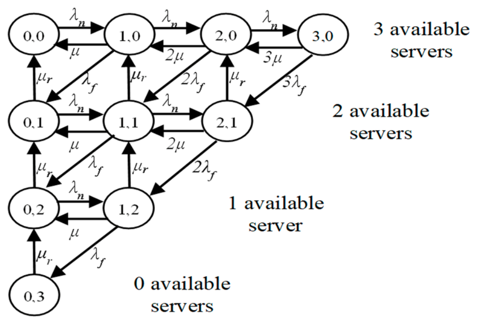
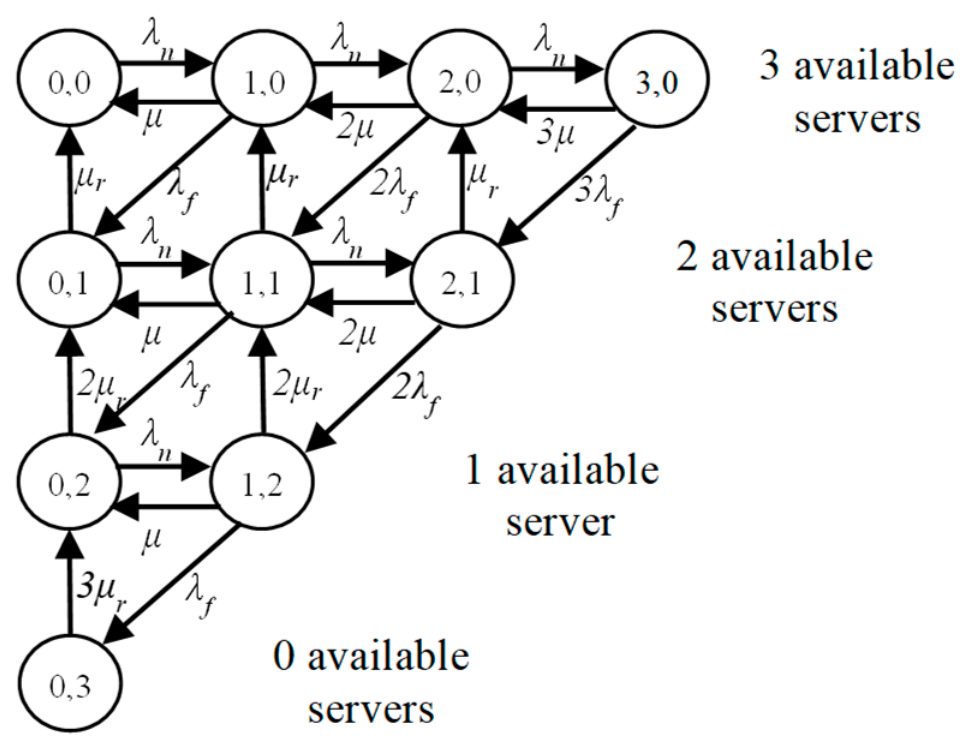
For presentation purposes, we consider a system of C = 3 servers, λ_n = μ = λ_f = 1 and μ_r = 10 and let (n_b, n_f) be a state of the system, where n_b denotes the number of busy servers, and n_f denotes the number of failed servers, with n_b + n_f ≤ C. The corresponding 2D continuous-time Markov chain consists of (C + 1)(C + 2)/2 = 10 states of the form (n_b, n_f) (see Figure 1) [30].

According to Figure 1, we observe that (1) the vertical “μ_r” transitions (e.g., from state (0, 3) to (0, 2)) refer to the single repair facility that is shared by all failed servers; (2) the non-recovery of ongoing calls is depicted by the “μ_r” transitions from a state (n_b, n_f) to a state (n_b, n_f − 1); and (3) each horizontal line can be considered as a loss system with the corresponding available servers.

2.2. The Exact Method for the Shared Repair Case

The exact method provides exact CBP results but requires knowledge of the state space of the system and the solution of the set of linear GB equations for each state (n_b, n_f) expressed as rate into state (n_b, n_f) = rate out of state (n_b, n_f) in order to obtain the steady-state probabilities P(n_b, n_f).

If 0 < n_b < C and 0 < n_f < C, with n_b + n_f ≤ C, then the corresponding GB equation for state (n_b, n_f) is the following:

λ_nP(n_b − 1, n_f) + z(n_b + 1)μP(n_b + 1, n_f) + (n_b + 1)λ_fP(n_b + 1, n_f − 1) + zμ_rP(n_b, n_f + 1)
= (zλ_n + n_bλ_f + n_bμ + μ_r)P(n_b, n_f)

(1a)

where z = 0 when n_b + n_f = C; otherwise, z = 1.

Similarly, the GB equations when: (1) n_b = 0 and 0 < n_f < C, (2) 0 < n_b < C and n_f = 0, (3) n_b = C and n_f = 0, (4) n_b = 0 and n_f = C, and (5) n_b = 0 and n_f = 0, are:

μP(1, n_f) + λ_fP(1, n_f − 1) + μ_rP(0, n_f + 1) = (λ_n + μ_r) P(0, n_f)

(1b)

λ_nP(n_b − 1, 0) + (n_b + 1)μP(n_b + 1, 0) + μ_rP(n_b, 1) = (λ_n + n_bλ_f + n_bμ) P(n_b, 0)

(1c)

λ_nP(C − 1, 0) = (Cλ_f + Cμ) P(C, 0)

(1d)

λ_fP(1, C − 1) = μ_rP(0, C)

(1e)

μP(1, 0) + μ_rP(0, 1) = λ_n P(0, 0)

(1f)

Based on P(n_b, n_f), we compute the exact CBP, P_b,exact via:

$$P_{b, exact}={\displaystyle \sum _{n_b+n_f=C}P\left(n_b,n_f\right)}$$

(2)

In the case of our example, the solution of the 10 GB equations shown in Figure 1 gives [30]: P_b,exact = P(3, 0) + P(2, 1) + P(1, 2) + P(0, 3) = 0.01644.

The exact method requires the solution of (C + 1)(C + 2)/2 GB equations. Assuming that the system of GB equations is solved using an iterative sparse linear solver, its computational complexity is of the order of O(KC²), where K is the number of iterations required for convergence. The corresponding memory consumption is of the order of O(C²).

Before we proceed, note that the Erlang B formula, which determines the CBP in the Erlang loss model, P_C(a_n), given by

$$P_C\left(a_n\right)={\displaystyle \frac{a_n^C}{C!}}/{\displaystyle {\sum }_{i=0}^C\frac{a_n^i}{i!}}$$

(3)

fails to approximate the exact CBP results.

More specifically, the corresponding CBP results when a_n = 1.0 erl and C = 3 are: P₃(1.0) = 0.0625.

2.3. The Performability Method for the Shared Repair Case

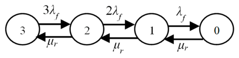
In the “performability method”, the 2D Markov chain in Figure 1 is approximated by two independent Markov chains [21,22]. The first Markov chain describes the server availability model, i.e., server failures and repairs (see Figure 2). The second one refers to the Erlang loss model, which is a pure performance model (see Figure 3).

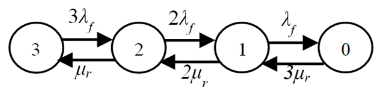
We initially consider the first Markov chain in Figure 2. Each state in the availability model in Figure 2 depicts the number of available (busy or idle) servers. Thus, a transition from state i to state i − 1 happens at rate iλ_f, i = 1, 2, 3, while a transition from state i to state i + 1 happens at rate μ_r (for i = 0, 1, 2). A transition from state i to state i − 1 at a rate of iλ_f implies that any of the i servers may fail, even if all servers are idle. This is an approximation of the exact model, in which only busy servers may fail. As an example, consider state C = 3 in Figure 2. Then, at a rate of 3λ_f, one of the three servers may fail. In Figure 1, the rate 3λ_f appears in the transition from state (3, 0) to (2, 1) (i.e., from a state with three busy servers to a state with two busy and one failed server).

By considering the local balance (LB) equations (rate-down = rate-up) between two adjacent states i and i − 1, we can determine the steady-state probabilities of the availability model for the shared repair case, $P_i^{av}$, i = 0…, C, via the formula [21]:

$$P_i^{av}={\displaystyle \frac{{\left(\frac{{\lambda }_f}{{\mu }_r}\right)}^{C-i}C!/i!}{{\displaystyle \sum _{j=0}^C{\left(\frac{{\lambda }_f}{{\mu }_r}\right)}^{j}C!/\left(C-j\right)!}}}$$

(4)

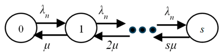
We now consider the second Markov chain, which refers to the Erlang loss model (see Figure 3). Each state in Figure 3 depicts the number of occupied servers, where s = 1, 2, …, C. In other words, for the availability model in Figure 2 there are C corresponding Erlang loss models depicted via Figure 3 [30].

The steady-state probabilities of the performance model (i.e., the Erlang loss model), $P_r^{per}$, r = 0…, s, are given by [2]:

$$P_r^{per}=\left({\left({\displaystyle \frac{{\lambda }_n}{\mu }}\right)}^r/r!\right)/\left({\displaystyle {\sum }_{j=0}^s{\left(\frac{{\lambda }_n}{\mu }\right)}^j/j!}\right)$$

(5)

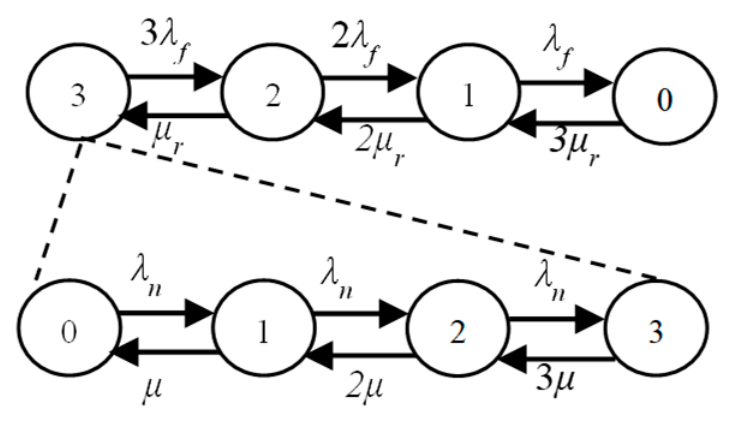
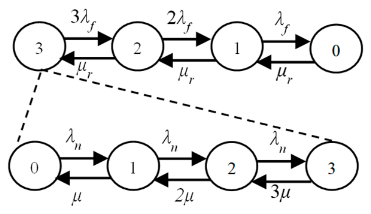
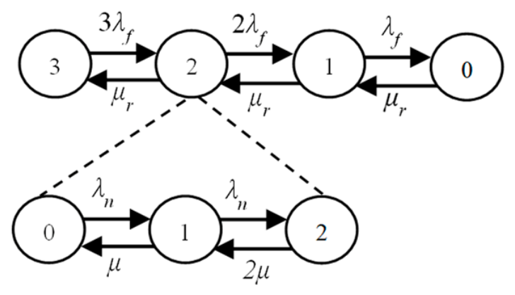
The two different models (the availability model of (4) and the performance model of (5)) are combined in the “performability method” under the assumption that for each state of the availability model, the corresponding performance model reaches a steady state. In other words, if we have C available servers in Figure 2, then s = C in Figure 3 and it is assumed that the system in Figure 3 reaches a steady state, which is essential for adopting (5) in the analysis of the “performability method” (as an example, see Figure 4 when C = 3, and Figure 5 when C = 2 available servers).

Based on (4) and (5), we determine the CBP according to the “performability method”, P_b,per, as follows [21]:

$$P_{b,per}=P_0^{av}+{\displaystyle \sum _{i=1}^C{P}_i^{av}\cdot P_i^{per}}$$

(6)

where the first term of (6) refers to the case of zero servers being available, while the second term refers to the case where i servers are available, and all of them are busy.

Based on (4)–(6), the computational complexity of the “performability method” is of the order of O(C²), since (5) (i.e., the Erlang loss formula) is computed for all possible numbers of available servers. The corresponding memory consumption is of the order of O(C).

In our example (C = 3, λ_n = μ_n = λ_f = 1 and μ_r = 10), we have P_b,per = 0.11603 (compare with the exact 0.01644).

2.4. The ΒΤ Method for the Shared Repair Case

The “BT method” is based on an aggregation technique initially proposed in [28]. According to this technique, we start by separating the state transition rates into fast and slow rates. The fast rates are of several orders of magnitude larger than the slow rates. Based on this, we assume that λ_n and μ_n are the fast rates, while λ_f and μ_r are the slow rates. Because of this assumption, we will see in Section 4 that when the values of λ_f and μ_r are comparable to the values of λ_n and μ_n, the BT method fails to approximate the exact CBP results.

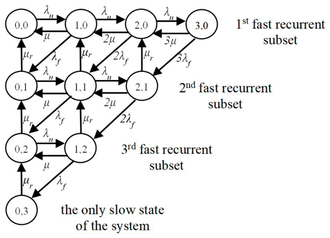
Based on the previous separation, the state space is divided into fast and slow states. Fast states are those that have at least one fast outgoing transition (e.g., in Figure 1, state (1, 0) has a fast outgoing transition, λ_n, to state (2, 0)). Slow states do not have fast outgoing transitions (e.g., in Figure 1, state (0, 3) is the only slow state).

Having defined fast and slow states, we continue by considering fast recurrent subsets of the 2D Markov chain. As an example, we will focus on Figure 1. The first C = 3 rows in Figure 1 form three fast recurrent subsets. The first recurrent subset consists of states (0, 0), (1, 0), (2, 0) and (3, 0). According to the BT method, the states inside a fast recurrent subset relate to each other via fast transitions (λ_n and μ in our case) and via slow transitions to any outside state (λ_f and μ_r in our case). As an example, the first recurrent subset is connected to the second fast recurrent subset (states: (0, 1), (1, 1) and (2, 1)) via the slow transitions λ_f and μ_r (see Figure 6).

Each of the C fast recurrent subsets is treated as a classical Erlang loss model of capacity s = 1, 2, …, C. For each subset, we can determine the values of $P_r^{per}$ via (5) and the expected number of busy servers, E(s), via:

$$E\left(s\right)={\displaystyle \frac{{\lambda }_n}{\mu }}\left(1-P_s^{per}\right) \mathrm{for} s =1,\dots ,C$$

(7)

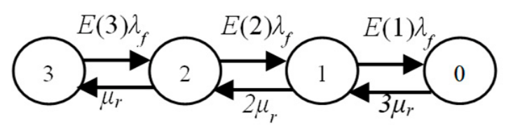
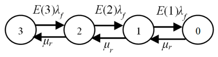
Having determined the values of E(s) for each of the fast recurrent subsets we can modify the pure availability model (where an idle or busy server may fail) to a BT-based availability model, where E(s) is adopted in order to ensure that only busy servers may fail (see Figure 7 when C = 3 and compare it with Figure 2 of the pure availability model).

Based on the above, we determine the steady-state probabilities of the BT-based availability model, $P_i^{BT}$, via [22]:

$$P_i^{BT}={\left({\displaystyle \frac{{\lambda }_f}{{\mu }_r}}\right)}^{C-i}{P}_C^{BT}{\displaystyle \prod _{s=i+1}^{C}E\left(s\right)}$$

(8)

where $P_C^{BT}=1/\left(1+{\displaystyle {\sum }_{j=0}^{C-1}{\left(\frac{{\lambda }_f}{{\mu }_r}\right)}^{C-j}{\displaystyle {\prod }_{s=j+1}^{C}E\left(s\right)}}\right)$.

Based on (5), (7) and (8), we can determine the CBP according to the “BT method”, P_b,BT, as follows [22]:

$$P_{b,BT}=P_0^{BT}+{\displaystyle \sum _{i=1}^C{P}_i^{BT}\cdot P_i^{per}}$$

(9)

where the form of (9) resembles that of (6).

Based on (5) and (7)–(9), the computational complexity of the “BT method” is of the order of O(C²), since (5) is computed for all possible numbers of available servers. The corresponding memory consumption is of the order of O(C).

In our example (C = 3, λ_n = μ_n = λ_f = 1 and μ_r = 10), we get P_b,BT = 0.0775 (better than the value of 0.11603 obtained via the “performability method” but still far from the exact 0.01644) [30].

2.5. The Proposed Method for the Shared Repair Case

In the proposed method, we modify the “BT method” as follows:

(1)

Each of the C fast recurrent subsets is treated as a classical Erlang loss model of capacity s = 1, 2, …, C. For each subset, we can determine the values of $P_r^{\prime per}$ via (10) and the expected number of busy servers, E′(s), via (11):

$$P_r^{\prime per}=\left({\left({\displaystyle \frac{{\lambda }_n}{{\mu }^{\prime }}}\right)}^r/r!\right)/\left({\displaystyle {\sum }_{j=0}^s{\left(\frac{{\lambda }_n}{{\mu }^{\prime }}\right)}^j/j!}\right)$$

(10)

$$E^{\prime }\left(s\right)={\displaystyle \frac{{\lambda }_n}{{\mu }^{\prime }}}\left(1-P_s^{\prime per}\right) \mathrm{for} s =1,\dots ,C$$

(11)

by assuming that the service rate is ${\mu }^{\prime }=\mu +{\lambda }_f$. The rationale behind this modification is the following. A server fails at rate λ_f, and therefore we assume that the time a server is busy can be shortened from h = 1/μ to $h^{\prime }=1/{\mu }^{\prime }=1/\left(\mu +{\lambda }_f\right)$.

(2)

The steady-state probabilities of the BT-based availability model, $P_i^{BT}$, are determined via (8), where E(s) is replaced by E′(s) given by (11).

Based on (8), (10) and (11), we can determine the CBP according to the proposed method, P_b,prop, as follows:

$$P_{b,prop}=P_0^{BT}+{\displaystyle \sum _{i=1}^C{P}_i^{BT}\cdot P_i^{\prime per}}$$

(12)

where the form of (12) is similar to that of (9).

In our example (C = 3, λ_n = μ = λ_f = 1 and μ_r = 10), we obtain P_b,prop = 0.01644, which is the exact value.

Based on the modification of the service rate, we propose the following formula for the exact determination of the steady-state probabilities P(n_b, n_f), where n_b denotes the number of busy servers and n_f the failed servers, with n_b + n_f ≤ C:

$$P\left(n_b,n_f\right)={\displaystyle \frac{{\left(a^{\prime }\right)}^{n_b}/n_b!}{{\displaystyle \sum _{k=0}^{C-n_f}{\left(a^{\prime }\right)}^k/k!}}}{P}_{C-n_f}^{BT}$$

(13)

where a′ = λ_n/(μ + λ_f).

In more detail, we start from the formula:

$$P\left(n_b,n_f\right)=P\left(n_b\left|n_f\right.\right)P\left(n_f\right)$$

(14)

where P(n_f) expresses the steady-state probability that exactly n_f servers have failed, and $P(n_b\left|n_f)\right.$ is the corresponding conditional probability of n_b busy servers given n_f failed servers.

In what follows, we will show that the two factors of the right-hand side of (13) coincide with the corresponding factors in (14).

The rationale behind the first term of (13) can be explained with the aid of Figure 1. Specifically, Figure 1 shows that LB between adjacent states does not hold; however, there exists a form of local flow balance across a level that separates two successive states. To this end, consider Figure 1 (where C = 3 servers) and assume that the system has two available servers and a single failed server (i.e., n_f = 1). Then, due to the local flow balance, the conditional probability of n_b, given n_f = 1 $P(n_b\left|n_f=1)\right.$, satisfies the formula for 0 ≤ n_b < C − 1:

$${\lambda }_{n}P(n_b\left|n_f=1)=(n_b+1)(\mu +{\lambda }_f)\right.P((n_b+1)\left|n_f=1)\right.$$

(15)

or generally, for 0 ≤ n_b < C − n_f:

$${\lambda }_{n}P(n_b\left|n_f)=(n_b+1)(\mu +{\lambda }_f)\right.P((n_b+1)\left|n_f)\right.$$

(16)

Assuming a fixed value of n_f, let $L_{n_b}$ denote a level that separates state (n_b, n_f) from state (n_b + 1, n_f). Then, the left-hand side of (16) represents the “upward” probability flow across $L_{n_b}$, due to call arrivals, and the right-hand side of (16) expresses the “downward” probability flow across $L_{n_b}$, due to service completion or server failures.

We can rewrite (16) in terms of $P(0\left|n_f)\right.$ as follows:

$$P(n_b\left|n_f\right.)={\left({\displaystyle \frac{{\lambda }_n}{\mu +{\lambda }_f}}\right)}^{n_b}{\displaystyle \frac{1}{n_b!}}P(0\left|n_f)\right.$$

(17)

or, assuming that a′ = λ_n/(μ + λ_f):

$$P(n_b\left|n_f\right.)={\displaystyle \frac{{\left(a^{\prime }\right)}^{n_b}}{n_b!}}{\displaystyle \frac{1}{{\displaystyle \sum _{k=0}^{C-n_f}{\left(a^{\prime }\right)}^k/k!}}}$$

(18)

which shows that the first factor of the right-hand side of (13) is equal to the corresponding factor of (14).

For the second factors of (13) and (14), we start by defining

$$P(n_f)={\displaystyle \sum _{n_b=0}^{C-n_f}P(n_b,n_f)} n_f = 0, 1,\dots ,C$$

(19)

To derive the GB equation for the (aggregated) state n_f, we sum the GB equations of states (0, n_f), (1, n_f), …, (C − n_f, n_f). During this summation, all transitions due to the arrivals of new calls and service completions (of in-service calls) cancel. As a result only failure and repair transitions between states n_f − 1, n_f and n_f + 1 remain. Based on the above, the GB equation for the (aggregated) state n_f (n_f = 1, …, C − 1) is the following:

$${\lambda }_f{\displaystyle {\displaystyle \sum _{n_b=1}^{C-(n_f-1)}}{n}_b}P(n_b,n_f-1) + {\mu }_{r}P(n_f+1)={\lambda }_f{\displaystyle {\displaystyle \sum _{n_b=1}^{C-n_f}}{n}_b}P(n_b,n_f) + {\mu }_{r}P(n_f)$$

(20)

By defining the conditional mean number of busy servers n_b, given n_f $E(n_b\left|n_f)\right.$ via:

$$E\left(n_b\left|n_f\right.\right)={\displaystyle \frac{{\displaystyle \sum _{n_b=1}^{C-n_f}{n}_b}P(n_b,n_f)}{P(n_f)}}$$

(21)

we can rewrite (20) as follows:

$${\lambda }_{f}E\left(n_b\left|n_f-1\right.\right)P(n_f-1) + {\mu }_{r}P(n_f+1)=({\lambda }_{f}E\left(n_b\left|n_f\right.\right) + {\mu }_r)P(n_f)$$

(22)

From (18), the conditional distribution $P(n_b\left|n_f)\right.$ is the occupancy distribution of an Erlang loss system with a′ = λ_n/(μ + λ_f) and capacity C − n_f. Thus, we can write:

$$E\left(n_b\left|n_f\right.\right)={\displaystyle \sum _{n_b=1}^{C-n_f}{n}_b}P\left(n_b\left|n_f\right.\right)={\displaystyle \frac{{\displaystyle \sum _{n_b= 1}^{C-n_f}\frac{{(a^{\prime })}^{n_b}}{(n_b-1)!}}}{{\displaystyle \sum _{k= 0}^{C-n_f}\frac{{(a^{\prime })}^k}{k!}}}}={\displaystyle \frac{a^{\prime }{\displaystyle \sum _{t= 0}^{C-n_f-1}\frac{{(a^{\prime })}^t}{t!}}}{{\displaystyle \sum _{k= 0}^{C-n_f}\frac{{(a^{\prime })}^k}{k!}}}}=a^{\prime }\left(1-{\displaystyle \frac{\frac{{(a^{\prime })}^{C-n_f}}{(C-n_f)!}}{{\displaystyle \sum _{k= 0}^{C-n_f}\frac{{(a^{\prime })}^k}{k!}}}}\right)$$

(23)

Based on (10) and (11), we can write (23) as follows:

$$E\left(n_b\left|n_f\right.\right)=a^{\prime }\left(1-P_{C-n_f}^{\prime per}\right)=E^{\prime }\left(C-n_f\right)$$

(24)

Substituting (24) in (22) leads to the following equation for n_f = 1, …, C − 1:

$${\lambda }_f{E}^{\prime }(C-n_f+1)P(n_f-1) + {\mu }_{r}P(n_f+1)=({\lambda }_f{E}^{\prime }(C-n_f) + {\mu }_r)P(n_f)$$

(25)

Since the (aggregated) system contains C servers and n_f of them are the failed servers, we have i = C − n_f available servers. Let Q_i be the probability that i servers are available in the (aggregated) system. Thus,

$$Q_i=P(C-i)=P(n_f)$$

(26)

and

$$E^{\prime }(C-n_f)=E^{\prime }(i)$$

(27)

Based on (26) and (27), we may rewrite (25) as follows:

$${\lambda }_f{E}^{\prime }(i+1)Q_{i+1}+ {\mu }_r{Q}_{i-1}=({\lambda }_f{E}^{\prime }(i) + {\mu }_r)Q_i, 1\le i\le C-1$$

(28)

Equation (28) is the GB equation of state i in the modified BT model. For the boundary states n_f = 0 (or i = C) and n_f = C (or i = 0), we can write (29) and (30), respectively:

$${\lambda }_f{E}^{\prime }(C)Q_C= {\mu }_r{Q}_{C-1}$$

(29)

$${\lambda }_f{E}^{\prime }(1)Q_1= {\mu }_r{Q}_0$$

(30)

Equations (28)–(30) are identical to the GB equations of the modified BT model. Thus, the probability distribution Q_i coincides with the corresponding distribution of the modified BT model, i.e., $Q_i=P_i^{BT}$ for i = 0, 1, …, C or

$$Q_{C-n_f}=P(n_f)=P_{C-n_f}^{BT}$$

(31)

which shows that the second factor of the right-hand side of (13) equals the corresponding factor of (14).

Based on (8) and (10)–(12), the computational complexity and the memory consumption of the proposed method are the same as those of the “performability method” and the “BT method”.

In the case of our example and based on (13), we have the following values for all P(n_b, n_f): P(0, 0) = 0.577715, P(0, 1) = 0.028885, P(0, 2) = 0.001444, P(0, 3) = 0.000072, P(1, 0) = 0.288857, P(1, 1) = 0.014443, P(1, 2) = 0.000722, P(2, 0) = 0.072214, P(2, 1) = 0.003611 and P(3, 0) = 0.012036.

Based on (13), we can also determine the average number of busy servers, E_busy, and the average number of failed servers, E_failed, via (32) and (33), respectively:

$$E_{busy}={\displaystyle \sum _{n_b= 1}^C{\displaystyle \sum _{n_f= 0}^{C-n_b}{n}_b}}P\left(n_b,n_f\right)$$

(32)

$$E_{failed}={\displaystyle \sum _{n_f= 1}^C{\displaystyle \sum _{n_b= 0}^{C-n_f}{n}_f}}P\left(n_b,n_f\right)$$

(33)

In the case of our example (C = 3, λ_n = μ = λ_f = 1 and μ_r = 10), we have: E_busy = 0.49178 and E_failed = 0.05149.

In

Table 2. Execution times (in s) for the exact and the proposed methods.

	Exact Method	Proposed Method
C = 5 (no. states = 21)	0.006	0.00005
C = 10 (no. states = 66)	0.015	0.00007
C = 20 (no. states = 231)	0.035	0.0001
C = 40 (no. states = 861)	0.099	0.0002
C = 80 (no. states = 3321)	0.361	0.0005
C = 160 (no. states = 13,041)	1.433	0.0031
C = 320 (no. states = 51,681)	5.709	0.0109

, we present, for comparison, the execution times (in s) of the exact and the proposed methods for a system with λ_n = μ = λ_f = 10 and μ_r = 100 and various values of C. The results in Table 2 were obtained on a computer with an Intel(R) Core(TM) i7-1185G7 CPU @3.0 GHz and 16Gb RAM. Based on Table 2, it is obvious that, as C increases, the proposed method outperforms the exact method, which requires the solution of the corresponding linear systems of GB equations.

3. The Erlang Loss Model with Server Failures and Non-Shared Repair

3.1. Description of the Model

The main difference from the model of Section 2.1 is the fact that we consider one repair facility for each server. Therefore, we have the so-called non-shared repair case, in which each server undergoes repair as soon as it fails, independently of the other servers [18].

For presentation purposes, we consider again the simple example of Section 2.1 and present in Figure 8 the corresponding 2D Markov chain for the non-shared repair case.

Based on Figure 8, we observe that (1) the non-shared repair case is depicted by the vertical “n_f μ_r” transitions from a state (n_b, n_f) to a state (n_b, n_f − 1); (2) the non-recovery of ongoing calls is depicted by the fact that we do not have “n_f μ_r” transitions from a state (n_b, n_f) to a state (n_b + 1, n_f − 1); and (3) each horizontal line can be considered as a loss system with the corresponding available servers.

3.2. The Exact Method

The exact method provides exact CBP results but requires knowledge of the state space of the system and the solution of the corresponding set of GB equations in order to obtain the values of P(n_b, n_f).

If 0 < n_b < C and 0 < n_f < C, with n_b + n_f ≤ C, then the corresponding GB equation for state (n_b, n_f) is the following:

λ_nP(n_b − 1, n_f) + z(n_b + 1)μP(n_b + 1, n_f) + (n_b + 1)λ_fP(n_b + 1, n_f − 1) + z(n_f + 1)μ_rP(n_b, n_f + 1) =
(zλ_n + n_bλ_f + n_bμ + n_fμ_r)P(n_b, n_f)

(34a)

where z = 0 when n_b + n_f = C; otherwise, z = 1.

Similarly, the GB equations when: 1) n_b = 0 and 0 < n_f < C, 2) 0 < n_b < C and n_f = 0, 3) n_b = C and n_f = 0, 4) n_b = 0 and n_f = C, and 5) n_b = 0 and n_f = 0, are

μP(1, n_f) + λ_fP(1, n_f − 1) + (n_f + 1)μ_rP(0, n_f + 1) = (λ_n + n_f μ_r) P(0, n_f)

(34b)

λ_nP(n_b − 1, 0) + (n_b + 1)μP(n_b + 1, 0) + μ_rP(n_b, 1) = (λ_n + n_bλ_f + n_bμ) P(n_b, 0)

(34c)

λ_nP(C − 1, 0) = (Cλ_f + Cμ) P(C, 0)

(34d)

λ_fP(1, C − 1) = Cμ_rP(0, C)

(34e)

μP(1, 0) + μ_rP(0, 1) = λ_n P(0, 0)

(34f)

Based on P(n_b, n_f), we compute the exact CBP, P_b,exact via:

$$P_{b, exact}={\displaystyle \sum _{n_b+n_f=C}P\left(n_b,n_f\right)}$$

(35)

If λ_n = μ = 1 and λ_f = μ_r = 0.1, then the solution of the 10 GB equations in Figure 8 gives: P_b,exact = P(3, 0) + P(2, 1) + P(1, 2) + P(0, 3) = 0.18304. For comparison, the model of Section 2.1, which considers the shared repair case, gives a value of P_b,exact = 0.29088, while the corresponding CBP obtained using the Erlang B formula (see (3)) for a_n = 1.0 erl and C = 3 is P₃(1.0) = 0.0625. Based on this example, the analysis of the non-shared repair case is necessary since the existing models cannot adequately describe the non-shared repair model.

3.3. The Performability Method for the Non-Shared Repair Case

Based on Section 2.3, we consider again the “performability method” for the non-shared repair case. More specifically, the 2D Markov chain in Figure 8 is approximated by two independent Markov chains. The first one shows the server availability model, i.e., server failures and the corresponding repairs (Figure 9). The second one refers to the Erlang loss model, which is a pure performance model (see Figure 3).

We initially consider the Markov chain in Figure 9, where each state expresses the number of available (busy or idle) servers. Thus, a transition from state i to state i − 1 happens at rate iλ_f, i =1, 2, 3, while a transition from state i to state i + 1 happens at rate (C − i)μ_r, i = 0, 1, 2. A transition from state i to state i − 1 at a rate of iλ_f implies that any of the i servers may fail, even if all servers are idle.

By considering the LB equations (rate-down = rate-up) between two adjacent states i and i − 1, we can determine the steady-state probabilities of the availability model for the non-shared repair case, $P_i^{av,ns}$, i = 0, …, C, as follows:

States C and C − 1:

$$C\cdot {\lambda }_f\cdot P_C^{av,ns}={\mu }_r\cdot P_{C-1}^{av,ns}\to P_{C-1}^{av,ns}={\displaystyle \frac{{\lambda }_f}{{\mu }_r}}\cdot C\cdot P_C^{av,ns}$$

States C − 1 and C − 2:

$$\left(C-1\right)\cdot {\lambda }_f\cdot P_{C-1}^{av,ns}=2{\mu }_r\cdot P_{C-2}^{av,ns}\to P_{C-2}^{av,ns}={\displaystyle \frac{C\cdot \left(C-1\right)}{2}}{\left({\displaystyle \frac{{\lambda }_f}{{\mu }_r}}\right)}^2\cdot P_C^{av,ns}$$

States C − 2 and C − 3:

$$\left(C-2\right)\cdot {\lambda }_f\cdot P_{C-2}^{av,ns}=3{\mu }_r\cdot P_{C-3}^{av,ns}\to P_{C-3}^{av,ns}={\displaystyle \frac{C\cdot \left(C-1\right)\cdot \left(C-2\right)}{3!}}{\left({\displaystyle \frac{{\lambda }_f}{{\mu }_r}}\right)}^3\cdot P_C^{av,ns}$$

and generally:

$$P_{C-k}^{av,ns}={\displaystyle \frac{C\cdot \left(C-1\right)\cdot \left(C-2\right)\cdots \left(C-k+1\right)}{k!}}{\left({\displaystyle \frac{{\lambda }_f}{{\mu }_r}}\right)}^k\cdot P_C^{av,ns}$$

(36)

By setting i = C − k, we can rewrite (36) as follows:

$$\begin{array}{c}{P}_i^{av,ns}={\displaystyle \frac{C\cdot \left(C-1\right)\cdots \left(i+1\right)}{\left(C-i\right)!}}{\left({\displaystyle \frac{{\lambda }_f}{{\mu }_r}}\right)}^{C-i}\cdot P_C^{av,ns} \mathrm{or}\\ P_i^{av,ns}=\left(\begin{array}{l}C\\ i\end{array}\right){\left({\displaystyle \frac{{\lambda }_f}{{\mu }_r}}\right)}^{C-i}\cdot P_C^{av,ns}\end{array}$$

(37)

but ${\displaystyle \sum _{i=0}^C{P}_i^{av,ns}}=1$, and based on (37) we have

$$P_C^{av,ns}{\displaystyle \sum _{i=0}^C\left(\begin{array}{l}C\\ i\end{array}\right){\left(\frac{{\lambda }_f}{{\mu }_r}\right)}^{C-i}}=1$$

(38)

By the binomial theorem, we have ${\displaystyle \sum _{i=0}^C\left(\begin{array}{l}C\\ i\end{array}\right){\left(\frac{{\lambda }_f}{{\mu }_r}\right)}^{C-i}}={\left(1+{\displaystyle \frac{{\lambda }_f}{{\mu }_r}}\right)}^C$, and therefore (38) can be written as follows:

$$P_C^{av,ns}={\left({\displaystyle \frac{{\mu }_r}{{\lambda }_f+{\mu }_r}}\right)}^C$$

(39)

Based on (39), we can rewrite (37) as follows:

$$P_i^{av,ns}=\left(\begin{array}{l}C\\ i\end{array}\right)\cdot {\left({\displaystyle \frac{{\mu }_r}{{\lambda }_f+{\mu }_r}}\right)}^i\cdot {\left({\displaystyle \frac{{\lambda }_f}{{\lambda }_f+{\mu }_r}}\right)}^{C-i}$$

(40)

We now consider the second Markov chain, which refers to the Erlang loss model, (see Figure 3). For the availability model in Figure 9 there are C corresponding (pure performance) Erlang loss models depicted via Figure 3. As far as the steady-state probabilities of the performance model (i.e., the Erlang loss model), $P_r^{per}$, r = 0, …, s, are concerned, they are given by (5).

The two different models (the availability model of (40) and the performance model of (5)) are combined in the “performability method for the non-shared repair case” under the assumption that for each state of the availability model, the corresponding performance model reaches a steady state. In other words, if we have C available servers in Figure 9, then s = C in Figure 3 and we assume that the loss system in Figure 3 reaches a steady state, which is essential for adopting (5) (as an example, see Figure 10 when C = 3).

Based on (5) and (40), we determine the CBP according to the “performability method for the non-shared repair case”, $P_{b,per}^{ns}$, as follows:

$$P_{b,per}^{ns}=P_0^{av,ns}+{\displaystyle \sum _{i=1}^C{P}_i^{av,ns}\cdot P_i^{per}}$$

(41)

where the first term of (41) refers to the case of having zero available servers, while the second term refers to the case of i available servers where all of them are busy.

In our example (C = 3, λ_n = μ_n = 1 and λ_f = μ_r = 0.1), we have $P_{b,per}^{ns}$ = 0.39531 (compare with the exact 0.18304).

3.4. The ΒΤ Method for the Non-Shared Repair Case

The “BT method for the non-shared repair case” is similar to the one presented in Section 2.4. The only difference is that the description of the method (e.g., the fast and slow rates and the corresponding states) is based on Figure 8 instead of Figure 1.

Based on the above, each of the C fast recurrent subsets of the non-shared repair case can be treated as a classical Erlang loss model of capacity s = 1, 2, …, C. For each subset, we can determine the values of $P_r^{per}$ via (5) and the expected number of busy servers, E(s), via (7).

Having determined the values of E(s) for each of the fast recurrent subsets, we can modify the pure availability model (where an idle or busy server may fail) to a BT-based availability model where E(s) is adopted in order to ensure that only busy servers may fail (see Figure 11 when C = 3 and compare it with Figure 9 of the pure availability model for the non-shared repair case).

By considering the LB equations (rate-down = rate-up) between two adjacent states i and i − 1, we can determine the steady-state probabilities of the BT-based availability model for the non-shared repair, $P_i^{BT,ns}$, i = 0, …, C, as follows

States C and C − 1:

$$E\left(C\right)\cdot {\lambda }_f\cdot P_C^{BT,ns}={\mu }_r\cdot P_{C-1}^{BT,ns}\to P_{C-1}^{BT,ns}={\displaystyle \frac{{\lambda }_f}{{\mu }_r}}\cdot E\left(C\right)\cdot P_C^{BT,ns}$$

States C − 1 and C − 2:

$$E\left(C-1\right)\cdot {\lambda }_f\cdot P_{C-1}^{BT,ns}=2{\mu }_r\cdot P_{C-2}^{BT,ns}\to P_{C-2}^{BT,ns}={\displaystyle \frac{E\left(C\right)\cdot E\left(C-1\right)}{2}}{\left({\displaystyle \frac{{\lambda }_f}{{\mu }_r}}\right)}^2\cdot P_C^{BT,ns}$$

States C − 2 and C − 3:

$$E\left(C-2\right)\cdot {\lambda }_f\cdot P_{C-2}^{BT,ns}=3{\mu }_r\cdot P_{C-3}^{BT,ns}\to P_{C-3}^{BT,ns}={\displaystyle \frac{E\left(C\right)\cdot E\left(C-1\right)\cdot E\left(C-2\right)}{3!}}{\left({\displaystyle \frac{{\lambda }_f}{{\mu }_r}}\right)}^3\cdot P_C^{BT,ns}$$

and generally:

$$P_{C-k}^{BT,ns}={\displaystyle \frac{E\left(C\right)\cdot E\left(C-1\right)\cdot E\left(C-2\right)\cdots E\left(C-k+1\right)}{k!}}{\left({\displaystyle \frac{{\lambda }_f}{{\mu }_r}}\right)}^k\cdot P_C^{BT,ns}$$

(42)

By setting i = C − k, we can rewrite (42) as follows:

$$P_i^{BT,ns}={\displaystyle \frac{E\left(C\right)\cdot E\left(C-1\right)\cdot E\left(C-2\right)\cdots E\left(i+1\right)}{\left(C-i\right)!}}{\left({\displaystyle \frac{{\lambda }_f}{{\mu }_r}}\right)}^{C-i}\cdot P_C^{BT,ns}$$

(43)

But ${\displaystyle \sum _{i=0}^C{P}_i^{BT,ns}}=1$ and based on (43) we have:

$$P_C^{BT,ns}={\left[1+{\displaystyle \sum _{i=0}^{C-1}\frac{{\left({\lambda }_f/{\mu }_r\right)}^{C-i}}{\left(C-i\right)!}{\displaystyle \prod _{s=i+1}^{C}E\left(s\right)}}\right]}^{-1}$$

(44)

Based on (44) we can rewrite (43) as follows:

$$P_i^{BT,ns}={\displaystyle \frac{1}{\left(C-i\right)!}}\cdot {\left({\displaystyle \frac{{\lambda }_f}{{\mu }_r}}\right)}^{C-i}\cdot P_C^{BT,ns}{\displaystyle \prod _{s=i+1}^{C}E\left(s\right)}$$

(45)

Based on (5), (44) and (45), we can determine the CBP according to the “BT method for the non-shared repair case”, $P_{b,BT}^{ns}$, as follows:

$$P_{b,BT}^{ns}=P_0^{BT,ns}+{\displaystyle \sum _{i=1}^C{P}_i^{BT,ns}\cdot P_i^{per}}$$

(46)

where the form of (46) resembles that of (41).

In our example (C = 3, λ_n = μ_n = 1, λ_f = μ_r = 0.1), we obtain $P_{b,BT}^{ns}$ = 0.21053 (better than 0.39531 obtained via the “performability method for the non-shared repair case” but still far from the exact 0.18304).

3.5. The Proposed Method for the Non-Shared Repair Case

In the proposed method, we modify the “BT method” as follows:

(1)

Each of the C fast recurrent subsets is treated as a classical Erlang loss model of capacity s = 1, 2, …, C. For each subset, we can determine the values of $P_r^{\prime per}$ via (10) and the expected number of busy servers, E′(s), via (11) under the assumption that the service rate is ${\mu }^{\prime }=\mu +{\lambda }_f$.

(2)

The steady-state probabilities of the BT-based availability model, $P_i^{BT,ns}$, are determined via (45) where E(s) is replaced by E′(s) given by (11).

Based on (10), (11) and (45) we can determine the CBP according to the proposed method, $P_{b,prop}^{ns}$, as follows:

$$P_{b,prop}^{ns}=P_0^{BT}+{\displaystyle \sum _{i=1}^C{P}_i^{BT}\cdot P_i^{\prime per}}$$

(47)

In our example (C = 3, λ_n = μ = 1, λ_f = μ_r = 0.1), we obtain $P_{b,prop}^{ns}$ = 0.18304, which is the exact value.

Based on the modification of the service rate, we propose the following formula (similar to (13)) for the determination of the steady-state probabilities P(n_b, n_f), where n_b denotes the number of busy servers and n_f the failed servers, with n_b + n_f ≤ C:

$$P\left(n_b,n_f\right)={\displaystyle \frac{{\left(a^{\prime }\right)}^{n_b}/n_b!}{{\displaystyle \sum _{k=0}^{C-n_f}{\left(a^{\prime }\right)}^k/k!}}}{P}_{C-n_f}^{BT,ns}$$

(48)

where a′ = λ_n/(μ + λ_f).

In the case of our example and based on (48), we have the following values for all P(n_b, n_f): P(0, 0) = 0.182721, P(0, 1) = 0.166110, P(0, 2) = 0.075505, P(0, 3) = 0.022880, P(1, 0) = 0.166110, P(1, 1) = 0.151009, P(1, 2) = 0.068640, P(2, 0) = 0.075505, P(2, 1) = 0.068640 and P(3, 0) = 0.022880.

Based on (48), we can also determine the average number of busy servers, E_busy, and the average number of failed servers, E_failed, via (32) and (33), respectively.

In the case of our example (C = 3, λ_n = μ_n = 1, λ_f = μ_r = 0.1), we have E_busy = E_failed = 0.74269.

4. Evaluation

In this section, we present two application examples for the loss systems under study.

In the first example, we consider a system of C = 20 servers and various values of λ_n, μ, λ_f and μ_r to investigate the accuracy of the “performability method” and the “BT method” compared to the proposed and the exact methods in the shared repair case. The latter requires the solution of a linear system of 231 GB equations.

In

Table 3. CBP results when C = 20 servers (1st application example).

	Exact Method & Proposed Method	Performability Method	BT Method
λf = 1.0, μr = 0.1	0.975	0.988903	0.9875
λf = 0.5, μr = 0.1	0.9625	0.977833	0.975
λf = 0.1, μr = 0.1	0.8625	0.890361	0.875
λf = 0.05, μr = 0.1	0.7375	0.784193	0.750
λf = 0.01, μr = 0.1	0.016687	0.170037	0.018255
λf = 1.0, μr = 1.0	0.75	0.890361	0.875
λf = 0.5, μr = 1.0	0.625	0.784193	0.750
λf = 0.1, μr = 1.0	0.007274	0.170037	0.018255
λf = 0.05, μr = 1.0	0.000342	0.010921	0.00060
λf = 0.01, μr = 1.0	0.000162	0.000238	0.000182
λf = 1.0, μr = 10.0	0.0000027	0.170037	0.018255
λf = 0.5, μr = 10.0	0.0000032	0.010921	0.00060
λf = 0.1, μr = 10.0	0.000057	0.000238	0.000182
λf = 0.05, μr = 10.0	0.000094	0.000189	0.000169
λf = 0.01, μr = 10.0	0.000143	0.000164	0.000161
λf = 1.0, μr = 100.0	9.9 × 10−9	0.000238	0.000183
λf = 0.5, μr = 100.0	0.0000007	0.000189	0.000169
λf = 0.1, μr = 100.0	0.000049	0.000164	0.000161
λf = 0.05, μr = 100.0	0.000088	0.000161	0.000160
λf = 0.01, μr = 100.0	0.000141	0.000159	0.000159

, we present the corresponding CBP results, assuming that λ_n = 8.0 and μ = 1.0. We also consider four different values of μ_r = 0.1, 1.0, 10.0 and 100.0, each presented for five different values of λ_f = 1.0, 0.5, 0.1, 0.05 and 0.01. As a comparison, the CBP results of the classical Erlang loss model are: P₂₀(8) = 0.000159. In all cases of Table 3, we observe that the “BT method” provides better CBP results compared to the “performability method”. However, both methods fail to approximate the exact values unless the failure or repair rates are at least two orders of magnitude different from the arrival and service rates.

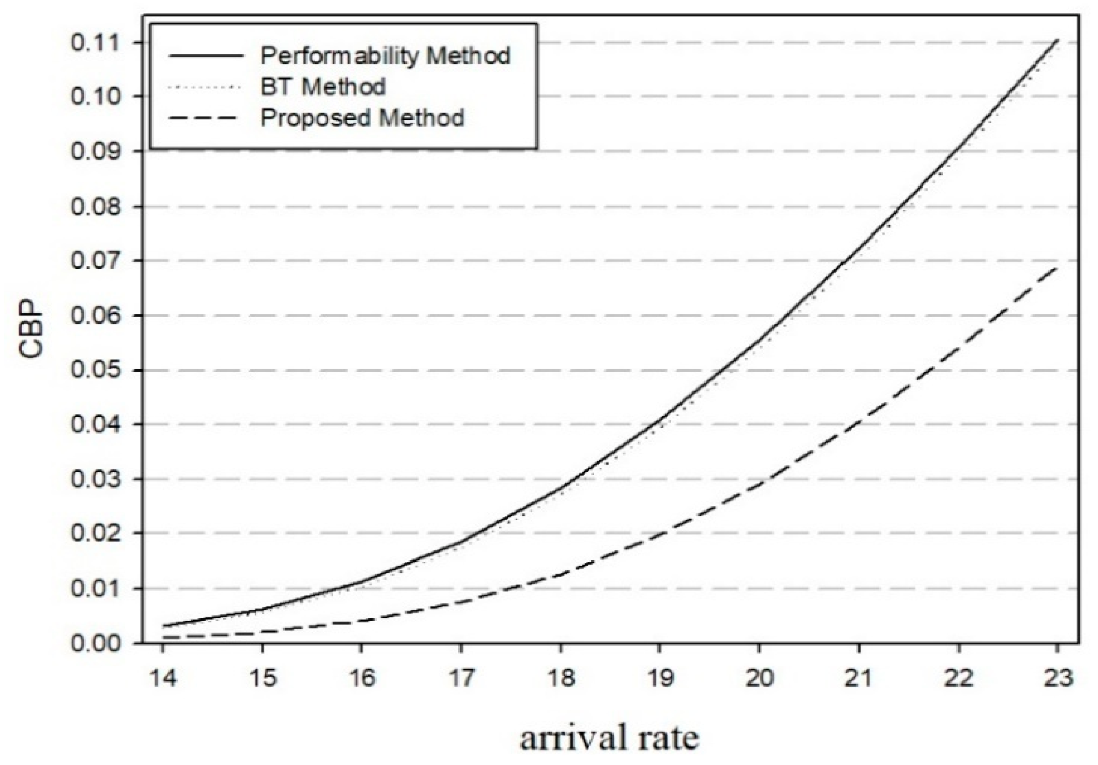
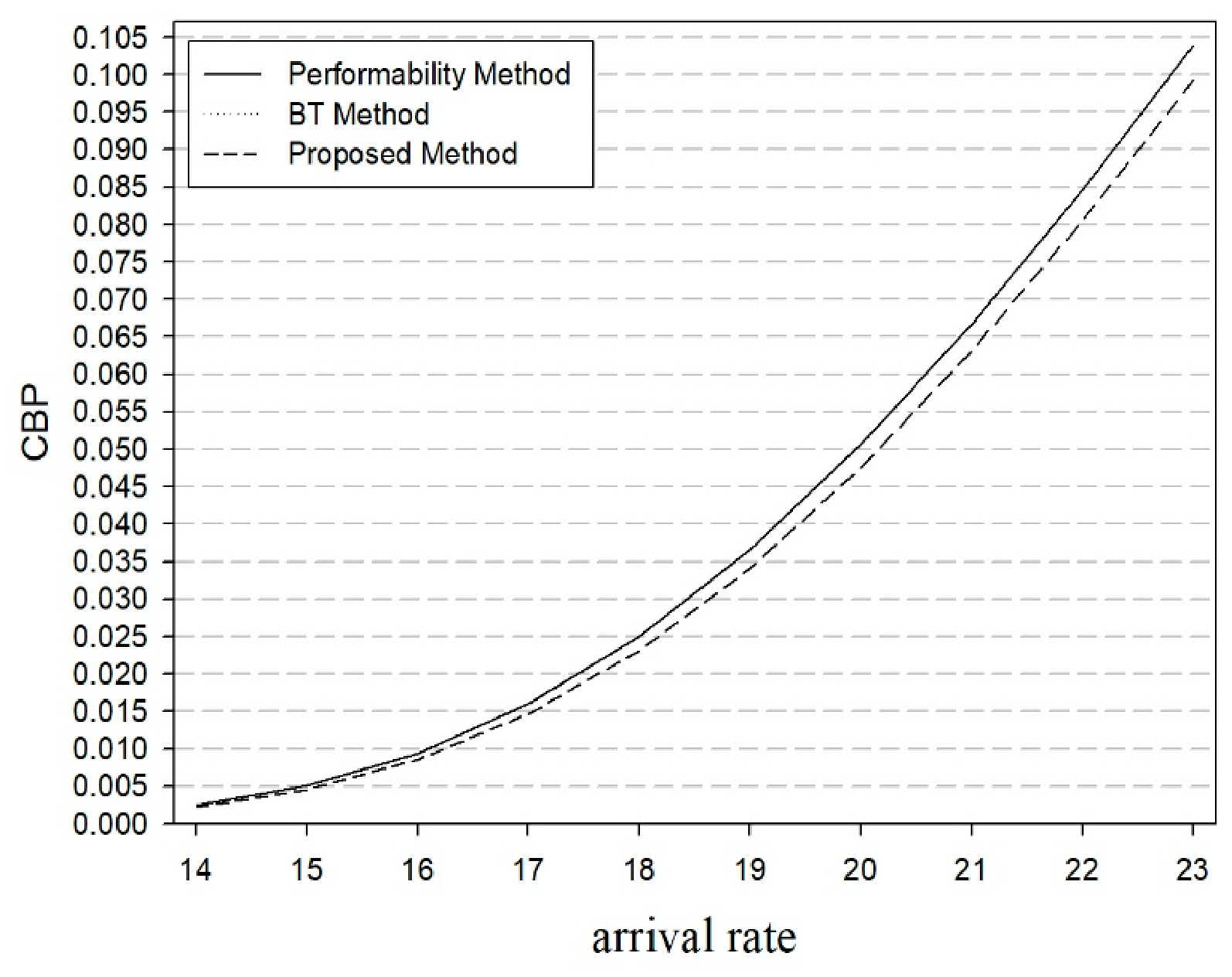
In the second example, we study again the shared repair case and consider a system of C = 25 servers, λ_n = 14.0, μ = 1.0, λ_f = 0.1, μ_r = 10. Figure 12 presents the CBP results of the “performability method”, the “BT method” and the proposed method (whose results are identical to the exact results obtained via the solution of 351 GB equations) for ten different values of λ_n (14.0, 15.0, …, 23.0). We observe that (1) an increase in λ_n results in an increase in CBP, and (2) both the “performability method” and the “BT method” fail to provide CBP results close to the exact results (which are obtained via the proposed method). In Figure 13, we consider the same example but for λ_f = 0.01. In that case, we observe that both methods provide quite good CBP results compared to those obtained via the proposed method.

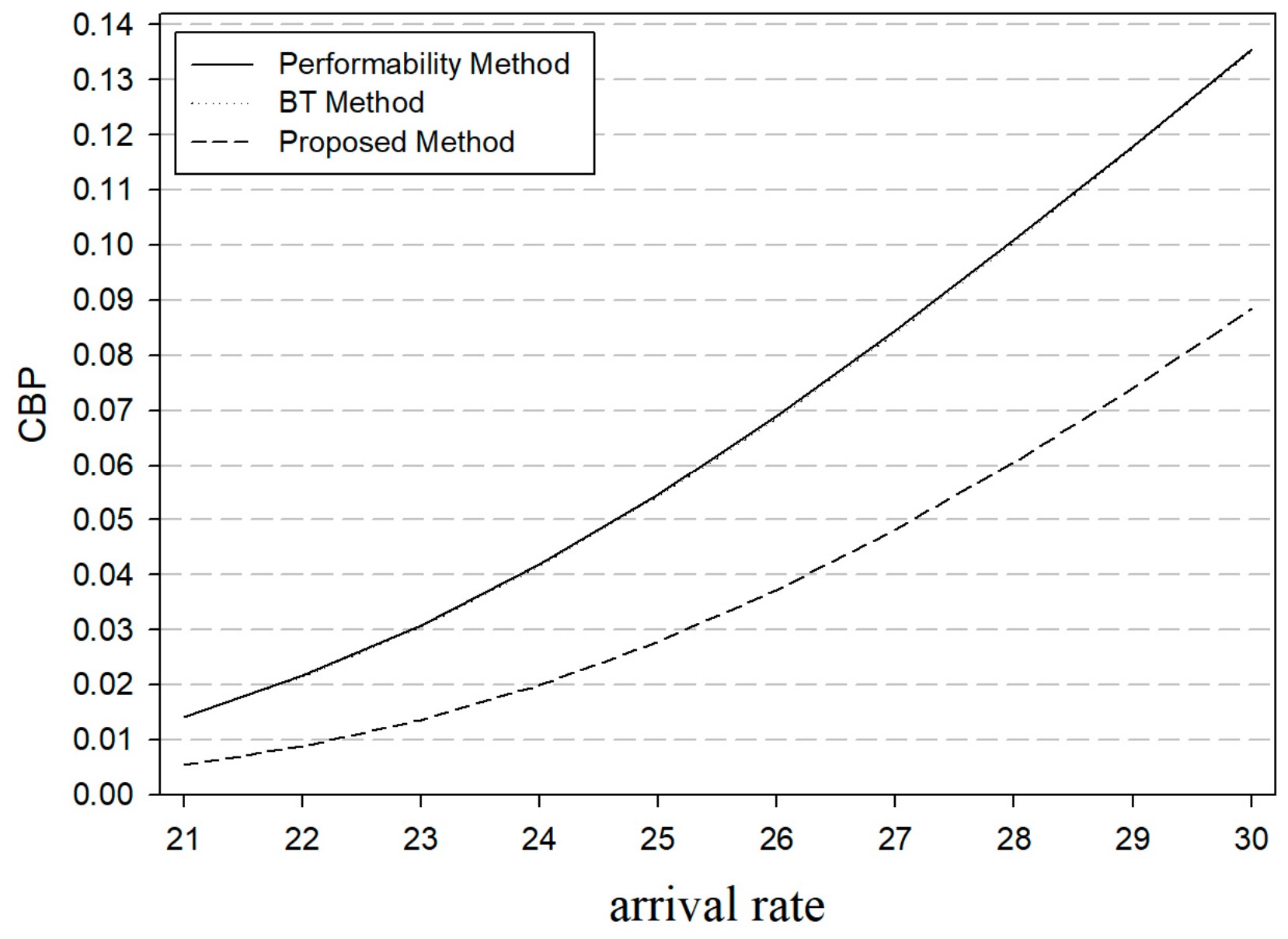
In the third example, we study the non-shared repair case and consider a system of C = 30 servers, λ_n = 21.0, μ = 1.0, λ_f = 0.1, μ_r = 20. Figure 14 presents the CBP results of the “performability method”, the “BT method” and the proposed method (whose results are identical to the exact results obtained via the solution of 496 GB equations) for ten different values of λ_n (21.0, 22.0, …, 30.0). We observe that an increase in λ_n results in an increase in CBP, and that both the “performability method” and the “BT method” fail to provide CBP results close to the exact results obtained via the proposed method. In

Table 4. CBP results when C = 30 servers (3rd application example).

	Non Shared Repair			Shared Repair
	Exact Method & Proposed Method	Perform. Method	BT Method	Exact Method & Proposed Method	Perform. Method	BT Method
λf = 1.0, μr = 20	0.000026	0.074747	0.070322	0.000504	0.295090	0.229522
λf = 1.0, μr = 30	0.000020	0.067146	0.064182	0.000050	0.130219	0.098926
λf = 1.0, μr = 40	0.000017	0.063420	0.061196	0.000026	0.086807	0.074039
λf = 1.0, μr = 50	0.000016	0.061213	0.059433	0.000020	0.072836	0.065996
λf = 1.0, μr = 60	0.000015	0.059752	0.058269	0.000017	0.066640	0.062247
λf = 0.1, μr = 20	0.027849	0.054720	0.054276	0.027998	0.055107	0.054516
λf = 0.1, μr = 30	0.027491	0.054011	0.053716	0.027554	0.054174	0.053817
λf = 0.1, μr = 40	0.027312	0.053658	0.053437	0.027347	0.053747	0.053493
λf = 0.1, μr = 50	0.027206	0.053447	0.053269	0.027227	0.053503	0.053305
λf = 0.1, μr = 60	0.027135	0.053306	0.053158	0.027150	0.053344	0.053182

, we present the corresponding CBP results for the shared and the non-shared repair cases, assuming that λ_n = 25.0 and μ = 1.0. We also consider five different values of μ_r = 20.0, 30.0, …, 60.0, each presented for two different values of λ_f = 1.0 and 0.1. As a comparison, the CBP results of the classical Erlang loss model are P₃₀(25.0) = 0.0526. In all cases in Table 4, we observe that the “BT method” provides better CBP results compared to the “performability method”. However, both methods fail to approximate the exact values. In addition, we observe that the CBP results of the non-shared repair loss model are always lower compared to the corresponding results of the shared repair loss model, which is anticipated, since the rate at which failed servers are repaired is higher in the non-shared repair case.

5. Conclusions

This paper studies an Erlang loss system with server availability, capturing the impact of server failures and repairs on CBP. Three methods are reviewed for the CBP determination in the case of the shared repair facility: an exact one based on a 2D Markov chain and two approximate approaches, the “performability method” and the “BT method”. In addition, one method is proposed which provides exact CBP results and is based on the “BT method”. In addition, we study and provide the corresponding analysis of all methods in the case of the non-shared repair facility. Analytical CBP results showed that the proposed method outperforms the approximate methods in both the shared and non-shared repair cases. Likewise, the “BT method” consistently provides better CBP results than the “performability method”, as it correctly accounts for failures of busy servers only. Both approximate methods are reliable when failure and repair rates differ sufficiently from arrival and service rates.

An interesting future research direction is the analysis of generally distributed failure and repair times. This would enable the study of the impact of different failures and repair time distributions on CBPs. Another interesting research direction is the analysis of retries of blocked calls (either due to an insufficient number of available servers or due to failed servers), which violate the assumption of Poisson arrivals and affect CBPs. Finally, other possible future extensions of this work are to consider the case of an arrival process other than the Poisson process (e.g., the case where traffic is generated by a finite number of users or the case of batched Poisson arrivals) as well as the important case of multirate traffic, where calls require more than a single server to be serviced.

References

1. Stasiak, M.; Głąbowski, M.; Wisniewski, A.; Zwierzykowski, P. Modeling and Dimensioning of Mobile Networks: From GSM to LTE; John Wiley: Hoboken, NJ, USA, 2011. [Google Scholar]
2. Moscholios, I.; Logothetis, M. Efficient Multirate Teletraffic Loss Models Beyond Erlang; John Wiley & IEEE Press: Hoboken, NJ, USA, 2019. [Google Scholar]
3. Weissenberg, J.; Weissenberg, M. Model of a queuing system with BPP elastic and adaptive traffic. IEEE Access 2022, 10, 130771–130783. [Google Scholar] [CrossRef] [Scilit]
4. Głąbowski, M.; Sobieraj, M.; Stasiak, M. Analytical modeling of groups of links in elastic optical networks. IEEE Access 2024, 12, 61073–61085. [Google Scholar] [CrossRef] [Scilit]
5. Gross, D.; Shortle, I.; Thompson, J.; Harris, C. Fundamentals of Queueing Theory, 5th ed.; Wiley: Hoboken, NJ, USA, 2018. [Google Scholar]
6. Cruz-Pérez, F.; Castellanos-López, S.; Hernández-Valdez, G. Queueing systems with fractional number of servers: Analysis and practical implementation of the Erlang-B traffic model. IEEE Access 2024, 12, 166268–166280. [Google Scholar] [CrossRef] [Scilit]
7. Yang, H.; Fu, J.; Wu, J.; Zukerman, M. A study of a loss system with priorities. Heliyon 2024, 10, e36109. [Google Scholar] [CrossRef] [Scilit] [PubMed]
8. Yao, L.; Yang, P.; Liu, Z.; Li, W.; Liu, J.; Ma, Z. Erlang model for multi-type data flow. IEEE Commun. Lett. 2025, 29, 1265–1269. [Google Scholar] [CrossRef] [Scilit]
9. Akimaru, H.; Kawashima, K. Teletraffic—Theory and Applications, 2nd ed.; Springer: Berlin/Heidelberg, Germany, 1999. [Google Scholar]
10. Gauthier, S.; Vasantam, T.; Vardoyan, G. On-demand resource allocation for a quantum network hub. IEEE Trans. Quantum Eng. 2026, 7, 4100330. [Google Scholar] [CrossRef] [Scilit]
11. Kaufman, J. Blocking in a shared resource environment. IEEE Trans. Commun. 1981, 29, 1474–1481. [Google Scholar] [CrossRef]
12. Kaufman, J.; Rege, K. Blocking in a shared resource environment with batched Poisson arrival processes. Perform. Eval. 1996, 24, 249–263. [Google Scholar] [CrossRef] [Scilit]
13. Vardakas, J.; Moscholios, I.; Logothetis, M.; Stylianakis, V. On code reservation in multi-rate OCDMA passive optical networks. In Proceedings of the 2012 8th International Symposium on Communication Systems, Networks & Digital Signal Processing (CSNDSP), Poznan, Poland, 18–20 July 2012. [Google Scholar]
14. Głąbowski, M.; Sobieraj, M.; Stasiak, M.; Dominik Stasiak, M. Modeling of Clos switching structures with dynamically variable number of active switches in the spine stage. Electronics 2020, 9, 1073. [Google Scholar] [CrossRef] [Scilit]
15. Głąbowski, M.; Sobieraj, M.; Stasiak, M. Analytical model of the connection handoff in 5G mobile networks with call admission control mechanisms. Sensors 2024, 24, 697. [Google Scholar] [CrossRef] [Scilit] [PubMed]
16. Ahmed, I.; Chatterjee, B.; Oki, E. AnalyticalSAR: Analytical modeling for blocking performance with security-aware reconfiguration in spectrally-spatially elastic optical networks. IEEE Trans. Netw. Serv. Manag. 2026, 23, 2935–2951. [Google Scholar] [CrossRef] [Scilit]
17. Hanczewski, S.; Stasiak, M.; Weissenberg, M. Determining resource utilization in cloud systems: An analytical algorithm for IaaS architecture. In Proceedings of the 2023 17th International Conference on Telecommunications (ConTEL), Graz, Austria, 11–13 July 2023. [Google Scholar]
18. Trivedi, K.; Bobbio, A. Reliability and Availability Engineering: Modeling, Analysis, and Application; Cambridge University Press: Cambridge, UK, 2017. [Google Scholar]
19. Kirsal, Y. Analytical modelling and optimization analysis of large-scale communication systems and networks with repairmen policy. Computing 2018, 100, 503–527. [Google Scholar] [CrossRef] [Scilit]
20. Kirsal, Y.; Ever, Y.; Mapp, G.; Raza, M. 3D analytical modeling and iterative solution for high performance computing clusters. IEEE Trans. Cloud Comput. 2022, 10, 2238–2251. [Google Scholar] [CrossRef] [Scilit]
21. Ma, Y.; Han, J.; Trivedi, K. Composite performance and availability analysis of communications networks. A comparison of exact and approximate approaches. In Proceedings of the IEEE Global Telecommunications Conference. Conference Record (Cat. No.00CH37137), San Francisco, CA, USA, 27 November–1 December 2000. [Google Scholar]
22. Ma, Y.; Han, J.; Trivedi, K. Composite performance and availability analysis of wireless communication networks. IEEE Trans. Veh. Technol. 2001, 50, 1216–1223. [Google Scholar] [CrossRef]
23. Kaufman, J. Blocking with retrials in a completely shared resource environment. Perform. Eval. 1992, 15, 99–113. [Google Scholar] [CrossRef] [Scilit]
24. Stamatelos, G.; Koukoulidis, V. Reservation-based bandwidth allocation in a radio ATM network. IEEE/ACM Trans. Netw. 1997, 5, 420–428. [Google Scholar] [CrossRef] [Scilit]
25. Moscholios, I.; Logothetis, M. Engset multirate state-dependent loss models with QoS guarantee. Int. J. Commun. Syst. 2006, 19, 67–93. [Google Scholar] [CrossRef] [Scilit]
26. Vassilakis, V.; Moscholios, I.; Logothetis, M. The extended connection-dependent threshold model for call-level performance analysis of multi-rate loss systems under the bandwidth reservation policy. Int. J. Commun. Syst. 2012, 25, 849–873. [Google Scholar] [CrossRef] [Scilit]
27. Hanczewski, S.; Weissenberg, J. Evaluation of the accuracy of the analytical model of a queuing system with a finite-compression mechanism in relation to real service disciplines. Electronics 2023, 12, 3343. [Google Scholar] [CrossRef] [Scilit]
28. Bobbio, A.; Trivedi, K. An aggregation technique for the transient analysis of stiff Markov chains. IEEE Trans. Comput. 1986, C-35, 803–814. [Google Scholar] [CrossRef] [Scilit]
29. Bobbio, A.; Trivedi, K. Computing cumulative measures of stiff Markov chains using aggregation. IEEE Trans. Comput. 1990, 39, 1291–1298. [Google Scholar] [CrossRef] [Scilit]
30. Lolis, K.; Vlasakis, M.; Moscholios, I.; Keramidi, I.; Uzunidis, D.; Bouloukakis, G.; Tselikas, N.; Logothetis, M. Performance evaluation of an Erlang loss system with server failures and a single repair facility. In Proceedings of the 2026 Panhellenic Conference on Electronics & Telecommunications (PACET), Patras, Greece, 23–24 April 2026. [Google Scholar]
Figure 1. State transition diagram of an Erlang loss model with C = 3 servers, including server failure and shared repair.
Electronics 15 03788 g001
Figure 2. State transition diagram of the pure availability model with C = 3 servers (shared repair case).
Electronics 15 03788 g002
Figure 3. State transition diagram of the Erlang loss model (a pure performance model) with s servers.
Electronics 15 03788 g003
Figure 4. The combination of the availability and the performance models in the “performability method” assuming C = 3 available servers (shared repair case).
Electronics 15 03788 g004
Figure 5. The combination of the availability and the performance models in the “performability method” assuming C = 2 available servers (shared repair case).
Electronics 15 03788 g005
Figure 6. Fast recurrent subsets and a slow state in the case of C = 3 servers (shared repair case).
Electronics 15 03788 g006
Figure 7. State transition diagram of the BT-based availability model with C = 3 servers (shared repair case).
Electronics 15 03788 g007
Figure 8. State transition diagram of an Erlang loss model with C = 3 servers, including server failure and non-shared repair.
Electronics 15 03788 g008
Figure 9. State transition diagram of the pure availability model with C = 3 servers (non-shared repair case).
Electronics 15 03788 g009
Figure 10. The combination of the availability and performance models in the “performability method”, assuming C = 3 available servers (non-shared repair case).
Electronics 15 03788 g010
Figure 11. State transition diagram of the BT-based availability model with C = 3 servers (non-shared repair case).
Electronics 15 03788 g011
Figure 12. CBP vs. arrival rate for the 2nd application example (λf = 0.1) and the shared repair case.
Electronics 15 03788 g012
Figure 13. CBP vs. arrival rate for the 2nd application example (λf = 0.01) and the shared repair case.
Electronics 15 03788 g013
Figure 14. CBP vs. arrival rate for the 3rd application example (μr = 20) and the non-shared repair case.
Electronics 15 03788 g014