Article

Green Vehicle Routing Model and Optimization Algorithm with Soft Time Window and Dynamic Demand

1
Business School, Hunan University, Changsha 410082, China
2
School of Intelligent Engineering and Intelligent Manufacturing, Hunan University of Technology and Business, Changsha 410205, China
*
Authors to whom correspondence should be addressed.
Electronics 2026, 15(17), 3780; https://doi.org/10.3390/electronics15173780
Submission received: 19 May 2026 / Revised: 13 August 2026 / Accepted: 18 August 2026 / Published: 24 August 2026

Abstract

This study investigates the dynamic-demand green vehicle routing problem with soft time windows (DDGVRPSTW). A two-stage optimization model is developed to minimize total distribution cost, including vehicle operating cost, fixed dispatch cost, fuel consumption cost, carbon emission cost, and time window penalty cost. To solve the model, a hybrid artificial bee colony state-transition algorithm (HABC-STA) is proposed. In the pre-optimization stage, multiple initial routes are generated and refined to obtain an initial distribution plan. In the dynamic optimization stage, customer information is updated at a specified event time, and four state-transition operators are used to search the neighborhood of the current solution and generate a revised routing plan with lower cost. Computational results on Solomon benchmark instances and a real-world case study show that the proposed method effectively reduces both total cost and environmental cost. The results also indicate that selecting an appropriate distribution scheme can significantly reduce fuel consumption and carbon emissions while improving overall routing efficiency.

1. Introduction

Logistics distribution is a critical component of economic activity. With the advancement of China’s carbon peaking and carbon neutrality goals, green logistics has attracted increasing attention from both academia and industry. In practice, however, customer demand is often dynamic and uncertain, which makes it difficult for vehicles to follow a fixed optimal route. As a result, distribution systems may experience higher operating costs, increased carbon emissions, and lower service quality. Traditional vehicle routing approaches are often not well suited to such dynamic environments. Therefore, studying the green vehicle routing problem under dynamic demand is of both theoretical and practical importance.
The dynamic vehicle routing problem (DVRP) arises when, after vehicles have departed from the distribution center, new customer requests emerge or the demands of existing customers change, requiring routes to be replanned in response to evolving operating conditions. This problem has been widely studied in the literature. Abdallah et al. formulated a capacity-constrained DVRP with the objective of minimizing total cost and proposed an improved genetic algorithm [1]. Further, Ulmer et al. investigated a VRP with stochastic customer demand, aiming to maximize the number of served customers, and developed an anticipatory dynamic strategy for the associated Markov decision process [2]. In addition, Pillac et al. considered newly arriving requests and capacity constraints in a total-cost minimization setting, proposed an event-driven framework for dynamic vehicle routing problems with stochastic demand, and designed a solution method combining a multi-scenario algorithm with online stochastic optimization [3]. Also, Li et al. developed a capacity-constrained DVRP to minimize total travel distance and solved it using a hybrid variable neighborhood artificial bee colony algorithm under a periodic real-time customer reset strategy [4]. Li et al. established a DVRP with time window constraints and employed an improved genetic algorithm to minimize travel distance [5]. Wang et al. further considered dynamic changes in new requests, existing demands, and customer locations, and proposed a multi-objective DVRP with time window constraints, which was solved using a dynamic evolutionary algorithm based on ensemble learning [6]. Despite these advances, most existing studies primarily focus on routing distance or distribution cost, while paying relatively limited attention to fuel consumption and carbon emissions.
The green vehicle routing problem (GVRP) was first proposed by Erdogan and Miller-Hooks [7] and primarily addresses fuel consumption and carbon emissions in logistics distribution. In recent years, this problem has been studied under a variety of optimization objectives. For example, Liu et al. developed a low-carbon VRP model with time window and vehicle capacity constraints and solved it using an improved ant colony algorithm based on road-segment partitioning [8]. Moreover, Cimen and Soysal minimized vehicle operating cost, travel time, and carbon emissions through a heuristic approach based on approximate dynamic programming [9]. Meanwhile, Andelmin et al. focused on minimizing total travel cost and route adjustment cost and proposed an exact algorithm based on subset inequalities to solve self-generated test instances [10]. Similarly, Yao et al. established a low-carbon VRP model with capacity constraints, aiming to minimize travel time and carbon emissions, and solved it using an improved particle swarm optimization algorithm [11]. Liu et al. [12] further formulated an optimization model to minimize distribution cost and carbon emission cost, partitioned road segments according to travel time, and solved the model using an improved ant colony algorithm. In addition, Zhao et al. considered traffic congestion zoning and developed a multi-vehicle-type GVRP model with time window, vehicle capacity, and fleet size constraints, which was solved using a hybrid differential evolution algorithm with the objective of minimizing carbon emission cost and vehicle management cost [13]. Likewise, Zhou et al. proposed a time-dependent green vehicle routing problem (TDGVRP) model with time window and vehicle capacity constraints to minimize fuel consumption, carbon emission cost, vehicle usage cost, labor cost, and fixed dispatch cost, and solved it using an improved ant colony algorithm [14]. Although these studies have incorporated factors such as carbon emissions, fuel consumption, travel distance, and time into green vehicle routing models and achieved promising results, relatively limited attention has been paid to dynamic customer demand.
In recent years, the green vehicle routing problem under dynamic demand has attracted growing attention. Jia et al. established an electric vehicle DVRP model based on a wait-and-see strategy, with the objective of minimizing total cost, and proposed a hybrid heuristic algorithm combining simulated annealing and variable neighborhood search [15]. Ge et al. considered urban restrictions on fuel vehicles and developed a two-stage electric vehicle DVRP model to minimize distribution cost, which was solved using a two-stage hybrid heuristic algorithm integrating an improved savings algorithm with tabu search [16]. Du et al. examined a delivery scenario in which company-owned vehicles and socially sourced vehicles jointly perform pickup and delivery tasks. They formulated a two-stage integer programming model for an electric vehicle DVRP in a crowdsourcing setting with the objective of minimizing total distribution cost and proposed an improved tabu-adaptive large neighborhood search algorithm [17]. Also, Guo et al. developed a GVRP model coupled with a dynamic traffic network and solved it using an improved Dijkstra algorithm [18]. Recently, Km developed a mathematical model for a multi-objective green vehicle routing problem, and proposed a dynamic adaptive large neighborhood search algorithm for optimizing bio-medical waste [19]. Nan et al. constructed a DVRP model with time windows to minimize total cost and proposed an improved adaptive large neighborhood search algorithm [20]. Although these studies have provided effective solution methods for dynamic-demand distribution problems involving either electric or fuel vehicles, relatively little attention has been paid to the joint consideration of customer satisfaction, fuel consumption, and carbon emission cost.
To address these gaps, this study considers the impact of travel distance and vehicle load on both fuel consumption and carbon emissions. A two-stage dynamic-demand green vehicle routing problem with soft time windows (DDGVRPSTW) is formulated under customer demand, vehicle capacity, and time window constraints, with the objective of minimizing total distribution cost, including fixed dispatch cost, travel cost, fuel consumption cost, carbon emission cost, and penalty cost. The soft time window setting provides greater flexibility in handling time constraints in dynamic routing scenarios. To solve the model efficiently, an improved artificial bee colony algorithm is developed by incorporating state-transition operators to enhance solution diversity and search performance. The proposed method is validated on Solomon benchmark instances and a real-world case study, demonstrating its effectiveness and practical applicability.
To address the above research gaps, this study explicitly considers the effects of travel distance and vehicle load on carbon emissions and total cost. A two-stage DDGVRPSTW is developed under soft time window, vehicle capacity, and customer demand constraints, with the objective of minimizing total distribution cost, fixed dispatch cost, fuel consumption cost, carbon emission cost, and penalty cost. The soft time window setting provides greater flexibility in handling time constraints in dynamic routing scenarios. To solve the model efficiently, an improved artificial bee colony algorithm (ABC) is developed, in which state-transition operators are incorporated to enhance solution diversity. The proposed approach is validated using both the standard Solomon benchmark instances and a real-world case study, thereby demonstrating the feasibility and effectiveness of the model and solution method. Although soft time window, ABC and load dependent emission have all been studied extensively, this work contributes a problem-specific integration rather than a simple recombination of existing components. This combination is designed specifically for the dynamic green routing setting considered in this study, where the interaction between scheduling flexibility and emission-aware routing has not been fully addressed by prior work. In contrast to prior studies that treat dynamic routing and green objectives separately, our method optimizes both within one search framework and evaluates them under the same solution representation.

2. Problem Description

A logistics distribution company operates a distribution center within a designated service area and provides delivery services to customers in that region. The center owns a certain number of delivery vehicles. All customers require the same category of goods, and all vehicles are assumed to be homogeneous. Customer locations and service time windows are known in advance, although they may vary across customers. Historical demand information is available, whereas actual customer demand is unknown and treated as a random variable. Before dispatch, each vehicle is loaded with sufficient goods and then follows a planned route to serve customers. Vehicles may arrive at customer locations before the beginning of the designated time windows, but service must be provided within the corresponding time windows. The objective of the distribution process is to minimize the total distribution cost of the distribution center. To formulate the DDGVRPSTW model, the following assumptions are made: (1) All nodes in the network are mutually reachable. Vehicles travel at a constant speed, and the effects of weather, traffic congestion, and other external factors are ignored. (2) The distribution network consists of one distribution center and multiple customer nodes, and the coordinates of all customer nodes remain unchanged throughout the distribution process. (3) Each vehicle departs from the distribution center and returns to the distribution center after completing its assigned service tasks. All delivery vehicles are of the same type. (4) Vehicle operation incurs travel cost, fuel consumption cost, carbon emission cost, and fixed dispatch cost. (5) The distribution center has sufficient inventory to satisfy actual customer demand, and stockout situations are not considered. (6) The load carried by each delivery vehicle cannot exceed its maximum capacity.

3. Mathematical Formulation of the DDGVRPSTW

3.1. Notation and Variables

To facilitate model establishment and solution, some notation and variables are shown in Table 1.

3.2. Two-Stage DDGVRPSTW Model Formulation

3.2.1. Pre-Optimization Stage Model

To capture the effects of travel distance and vehicle load on carbon emissions and total cost, a DDGVRPSTW model is formulated for the pre-optimization stage under soft time window, vehicle capacity, and customer demand constraints. As shown in Equation (1), the objective is to minimize total distribution cost, route adjustment cost, fuel consumption cost, carbon emission cost, and penalty cost. The soft time window penalty cost function is illustrated in Figure 1.
min z = C 1 + C 2 + C 3 + C 4 + C 5
where
C 1 = c 1 j H k K x 0 j k
C 2 = c 2 i U 1 j U 2 , i j k K d i j x i j k
C 3 = c 3 i U 1 j U 2 , i j k K f i j k x i j k d i j
C 4 = c 4 i U 1 j U 2 , i j k K e i j k x i j k d i j
p i = β 1 ( E i t i k ) + β 2 ( e i E i )         t i k < E i β 2 ( e i t i k ) E i t i k < e i 0 e i t i k l i , k K β 3 ( t i k l i ) l i < t i k L i β 3 ( L i l i ) + β 4 ( t i k L i )         t i k > L i
C 5 = i H p i
s . t .   i U 1 , i j k K x i j k = i U 1 , i j k K x j i k , j U 2
i H y i k 1 , k K
j H x 0 j k = i H x i ( r + 1 ) k = 1 , k K
j H b 0 j k x 0 j k i H q i , k K
i H q i y i k B , k K
t i j k = d i j v         i U 1 , j U 2 , k K , i j
t j k = t i k + s t i k + t i j k         i U 1 , j U 2 , k K , i j
t i k + s t i k + t i ( r + 1 ) k l r + 1         i U 1 , k K
i S j S x i j k S 1         S H , k K
q i 0 , x i j k 0 , 1 , y i k 0 , 1 ,   i U 1 , j U 2 , k K , i j
Equation (1) presents the objective function of the first stage, which aims to minimize the total comprehensive cost. Equations (2) and (3) correspond to the fixed dispatch cost and travel cost, respectively, while Equations (4) and (5) describe the fuel consumption cost and carbon emission cost. Equation (6) gives the penalty cost incurred by vehicle k at customer i, and Equation (7) aggregates the penalty cost over all vehicles. Equation (8) represents flow conservation at each customer node by requiring the number of incoming and outgoing vehicles to be equal. Equation (9) ensures that each customer is served by exactly one vehicle. Equation (10) requires each vehicle to depart from the distribution center and return to the depot after completing its service task. Equation (11) ensures that the total load carried by each vehicle when leaving the distribution center is no less than the total demand of the customers assigned to its route, whereas Equation (12) restricts the total demand served on each route to within the vehicle capacity. Equation (13) defines the travel time of vehicle k on arc (i,j), and Equation (14) specifies the arrival-time relationship between two consecutive customer nodes. Equation (15) imposes the time constraint on the return of vehicles to the distribution center. Equation (16) is used to eliminate sub-tours, and Equation (17) specifies the domains of the decision variables.

3.2.2. Dynamic Optimization Stage Model

During the delivery process, the arrival of new customer requests and changes in the demands of existing customers give rise to the dynamic optimization stage. Accordingly, the corresponding model is formulated in Equation (18). The total cost in the dynamic optimization stage consists of the cost incurred in the first stage, together with the fixed dispatch cost, travel cost, fuel consumption cost, carbon emission cost, and penalty cost generated by vehicle operations in the second stage.
min z = i A Z 0 i + C 1 + C 2 + C 3 + C 4 + C 5
where
C 1 = c 1 i N 3 j N 4 k M x i j k
C 2 = c 2 ( i N 1 j N 2 k K d i j x i j k + i N 3 j N 4 k M d i j x i j k )
C 3 = c 3 i N 3 j N 4 k M f i j k x i j k d i j c 3 j A k M f 0 j k x 0 j k d 0 j
C 4 = c 4 i N 3 j N 4 k M e i j k x i j k d i j c 4 j A k M e 0 j k x 0 j k d 0 j
Equation (19) denotes vehicle fixed cost. During the dynamic optimization stage, fixed costs include two parts: First, the fixed costs of vehicles that have departed from the distribution center, served customer points, and returned to the distribution center, as well as the fixed costs of vehicles that continue to serve customer points from virtual points during the service period. Second, the fixed costs of vehicles sent from the distribution center to provide service and return to the distribution center after completing the delivery task. Equation (20) represents the operating cost of the vehicle. During this period, the driving cost is the same as the cost mentioned above, which is the total driving cost of all dispatched vehicles in the two stages. Equation (21) represents the fuel consumption cost of the vehicle. The fuel consumption cost considered here is the sum of the two-stage comprehensive fuel consumption costs, but it is necessary to exclude the cumulative fuel consumption costs incurred by the vehicle from the self-distribution starting point to each point during the pre-optimization phase. Equation (22) is the carbon emission cost of the vehicle. The calculation principle for the carbon emission cost at this time is the same as that for fuel consumption cost.
The penalty cost C5 incurred by vehicle k at customer i, denoted by pi, and the total penalty cost of all vehicles are computed according to Equations (6) and (7), respectively. In addition to the constraints adopted in the pre-optimization stage model, the dynamic optimization stage model further includes the following constraints:
i N 2 x i j k = 1       i A , k R , i j
i F A 3 q i y i k b s k , k K
Equation (23) requires the original vehicles to depart from the corresponding virtual nodes in this stage, whereas Equation (24) ensures that the demand associated with each virtual node at the customer location does not exceed the remaining load capacity of the original vehicle.

3.3. Vehicle Carbon Emission Model

This study employs the MEET model [21] to estimate vehicle carbon emissions. The carbon emission rate of a vehicle, measured in g/km, is given as follows:
φ v = ω 0 + ω 1 v + ω 2 v 2 + ω 3 v 3 + ω 4 v + ω 5 v 2 + ω 6 v 3
where φ v denotes the carbon emission rate of an unloaded vehicle traveling at speed v on a level road, and ω 0 , ω 1 , ω 2 , ω 3 , ω 4 , ω 5 , ω 6 are constants determined by the vehicle type.
The load correction factor for the carbon emission rate is given as follows:
ψ = χ 0 + χ 1 γ + χ 2 γ 2 + χ 3 γ 3 + χ 4 v + χ 5 v 2 + χ 6 v 3 + χ 7 v
where γ denotes the ratio of the actual load carried by the vehicle on arc (i,j) to its capacity, and χ 0 , χ 1 , χ 2 , χ 3 , χ 4 , χ 5 , χ 6 , χ 7 are constants determined by the vehicle type.
Accordingly, the carbon emission rate of vehicle k, measured in kg/km, is given as follows:
c i j k = φ v ψ 1000
The carbon emission rate can be converted into the fuel consumption rate [21]. Given that 1 L of gasoline produces 2.32 kg of carbon emissions, the fuel consumption required to generate 1 kg of carbon emissions is 1/2.32 = 0.43 L. Accordingly, the fuel consumption rate of vehicle k on arc (i,j) is given as follows:
f i j k = c i j k 2.32

4. Solution Algorithm for the DDGVRPSTW Based on Artificial Bee Colony and State Transition

In the DDGVRPSTW model, customer demand is treated as a stochastic perturbation. Specifically, the realized demand of customer i at time t is expressed as q i t = q i + Δ q i t , where q i denotes the nominal demand and Δ q i t represents the random variation. In this study, Δ q i t is assumed to follow a normal distribution Δ q i t N μ i , σ i , where μ i and σ i denote the expected value and variance, respectively. To ensure feasibility, negative demand values are truncated to zero if necessary. This setting allows the model to capture uncertainty in customer demand while maintaining consistency with the benchmark instance.
In this paper, we treat customer demand as a random variable, using a normal distribution to describe demand fluctuations, and ensure that the demand is non-negative and an integer through truncation and rounding. In the simulation, a fixed random seed is used, and customer demand is sampled all at once at each dynamic moment for vehicle load feasibility assessment and route re-optimization. The level of demand fluctuation is set with a coefficient of variation of 0.2. When vehicles serve customers according to preplanned routes, route failure may occur if the remaining load of a vehicle is insufficient to meet actual customer demand, making route re-optimization necessary. To solve this problem, the proposed procedure is divided into two stages. In the first stage, a pre-optimization plan is generated based on the expected value and variance of customer demand. Specifically, a HABC-STA algorithm is employed to address the uncertainty associated with random customer demand. In pre-optimization stage, future customer demand trends are predicted based on historical demand data, which will result in an initial adaptive pre-optimized driving route scheme. In the second stage, the vehicle’s location is a virtual point at the dynamic moment T. The cargo amount of the vehicle is reassessed to determine whether it can continue to service customer points. If it cannot meet customer demands, new vehicles are dispatched from the distribution center to ensure all customer points are served. Additionally, the paths are continuously optimized during this stage to arrive at the final delivery route.

4.1. Initial Solution Generation

The algorithm adopts an integer encoding scheme. For example, the sequence “0-1-2-0-3-4-5-6-7-0-8-0” represents three vehicle routes, namely “0-1-2-0”, “0-3-4-5-6-0”, and “0-8-0”, where “0” denotes the distribution center and “1-8” denote eight customer nodes. The initial population is generated under the vehicle capacity constraint. Specifically, customers are assigned sequentially to the current route until the inclusion of customer j would violate the capacity limit. A new vehicle is then dispatched, and the assignment process continues in the same manner to generate an initial solution.

4.2. Pre-Optimization Route Generation

Step 1: Population initialization. The algorithm parameters are first initialized, including the population size N I N D , the maximum number of iterations M a x I t e r , the number of onlooker bees n g s b e e , the maximum allowable number of exploitations for the same nectar source L M , and the selection probabilities of the three state-transition operators p S w a p , p S h i f t , p S y m m e t r y . Initial solutions are then randomly constructed, with each individual representing an initial nectar source. For each individual, the encoded solution, the decoded routing plan, and the total cost are stored in a structure named chrom, where each routing plan represents a feasible solution to the problem. The exploitation count C of each nectar source is also recorded.
Step 2: Employed bee phase. To enhance the search capability of employed bees and reduce the risk of premature convergence to local optima, three operators from the state-transition algorithm are incorporated, namely the swap operator, shift operator, and symmetry operator. One of these operators is randomly selected to perform neighborhood search and generate a new solution. The detailed procedure is as follows.
Step 2.1: Neighborhood operation. A population denoted as State is first generated by applying a state-transition operator. A second state transition is then performed to obtain a new population, denoted as newState. The resulting population contains NIND × NIND/4 individuals. Each individual is decoded and evaluated using the objective function, and the individual with the minimum objective value is selected.
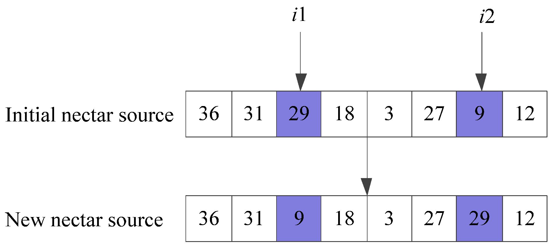
Swap operator. Two positions are selected at random, which are shown in blue color, and the elements at these positions are exchanged, as illustrated in Figure 2. For example, given an initial nectar source “36-31-29-18-3-27-9-12”, if positions 3 and 7 are randomly selected, the new nectar source obtained after the swap operation is “36-31-9-18-3-27-29-12”.
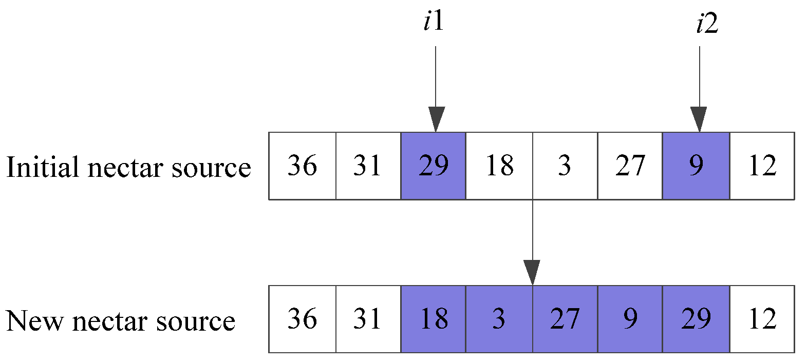
Shift operator. Two positions are selected at random, and the element at the first position is shifted to the position immediately after the element at the second position, as illustrated in Figure 3. For example, if positions 3 and 7 are randomly selected, moving the element at the first position yields the new nectar source “36-31-18-3-27-9-29-12”. The blue region denotes two randomly generated positions and the operation position.
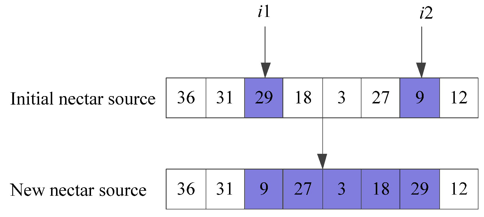
Symmetry operator. Two positions are selected at random, and all elements between these two positions are reversed, as illustrated in Figure 4. For example, if positions 3 and 7 are randomly selected, reversing the elements between these two positions yields the new nectar source “36-31-9-27-3-18-29-12”. The blue region denotes two randomly generated positions and the operation position.
Step 2.2: Greedy criterion. The objective value of each individual obtained from neighborhood search is compared with that of the corresponding initial solution. If the new solution has a smaller objective value, the solution is updated; otherwise, the exploitation count of the original nectar source is increased by 1.
Step 3: Onlooker bee phase. According to the fitness values of the individuals, onlooker bees are recruited using the roulette-wheel selection method to choose higher-quality nectar sources.
Step 3.1: Fitness evaluation of nectar sources.
The objective value of each individual is first calculated according to Equation (1). The fitness value of the i-th individual is then computed using Equations (29) and (30).
f i t ( i ) = 1 / C h r o m ( i ) . c u r r Cos t
P ( i ) = f i t ( i ) s u m ( f i t ( i ) )
In Equation (29), f i t ( i ) denotes the fitness value of each individual, and C h r o m ( i ) . c u r r Cos t denotes the total cost associated with each individual. In Equation (30), P ( i ) denotes the selection probability of each individual.
Step 3.2: Neighborhood search. As in the employed bee phase, the same three state-transition operators are used in this stage. The new population new state contains N I N D individuals. Each individual then undergoes the swap, shift, and symmetry operations to generate new nectar sources, after which a greedy selection procedure is performed by comparing the objective values of the new and original nectar sources.
Step 4: Scout bee phase. The exploitation count of each nectar source is examined to determine whether it exceeds the limit L M . If the exploitation count of a nectar source exceeds L M , a new nectar source is generated randomly, and its exploitation count is reset to 0. The algorithm then proceeds to Step 5.
Step 5: Individual update. The current best solution is recorded based on the objective value. If the number of updates reaches the maximum number of iterations M a x I t e r , the update process terminates and the optimal solution is obtained, after which the algorithm proceeds to Step 6. Otherwise, the algorithm returns to Step 2.
Step 6: Dynamic update after the pre-optimization stage.
After the delivery tasks in the pre-optimization stage are completed, a time point T is generated under the update strategy, at which dynamic changes occur. The dynamic update is triggered once at a pre-specified time point T, which is given in advance by the benchmark setting. In our implementation, T is treated as a fixed event time rather than a randomly generated or periodically scheduled time point. When the current simulation time reaches T, the prepare procedure is invoked to identify the customers already served, the vehicles currently in transit, and the remaining unserved customers, which are then passed to the dynamic re-optimization stage. The specific type of dynamic change activated after T is randomly selected by the update module, but the triggering time itself is fixed and reproducible. At this time, new customer nodes may appear, and the demand of originally unserved customers may also change. The current position of each vehicle is then calculated and treated as a virtual depot, and the corresponding set of virtual nodes is denoted by A. Considering the remaining load of vehicle k , denoted by b s k , it is further determined whether the vehicle is currently serving a customer node. If the vehicle is serving a customer, the elapsed service time is calculated. Finally, the set of served customers, the set of unserved customers, and the total cost Z 0 i generated at the end of the first stage are obtained as outputs.
Although swap, shift, and symmetry are classical local operators, their integration into the ABC framework enables a more balanced exploration–exploitation process, which can lead to better route refinement and reduced sensitivity to local optima.

4.3. Dynamic Optimization Route Generation

In the DDGVRPSTW problem, customer information may change when a dynamic update occurs at time point T. Such changes may cause the remaining load of a vehicle to become insufficient to meet the demands of subsequent customers on its route. In this case, the current vehicle location is treated as a virtual node and the routes for newly added customers and originally unserved customers are reoptimized.
Step 7: Considering four types of dynamic updates. Four dynamic update factors are considered, namely order cancelation, changes in the demand of existing customers, changes in the time windows of existing customers, and the arrival of new customer nodes. At each update, at least one and at most four of these factors are selected according to a given probability. The number of unserved customers in the dynamic stage and the distance matrix among all relevant nodes are then updated accordingly.
Step 8: Parameter initialization. The relevant data of newly added customers and unserved customers are first extracted, after which the algorithm parameters are initialized, including the population size D N I N D , the maximum number of iterations D M a x I t e r , the number of onlooker bees D n g s b e e , and the maximum allowable number of exploitations for the same nectar source D L M . Initial solutions are then randomly constructed, with each individual representing an initial nectar source. For each individual, the encoded solution, the decoded routing plan, and the total cost are stored in a structure named D C h r o m , where each routing plan represents a feasible solution to the problem. It is then determined whether the individual corresponds to a non-empty set. If so, the vehicles continuing service from the first stage are insufficient to satisfy the demands of all remaining customer nodes, and additional vehicles must be dispatched from the distribution center. Otherwise, the existing vehicles are sufficient to meet the remaining demand, and no additional dispatch is needed. The exploitation count D C of each nectar source is also recorded.
Step 9: Employed bee phase. In this stage, four operators are incorporated, namely the inter-route crossover operator ( D C r o s s o v e r ), the inter-route 2-opt operator ( D 2 o p t ), the intra-route swap operator ( D S w a p ), and the intra-route reversal operator ( D R e v e r s i o n ). One of these operators is randomly selected to perform neighborhood search and generate a new solution. The applicable operator depends on the number of customers in the route. If the route contains at least two customers, all four operators can be used; otherwise, only inter-route transformations are permitted. The resulting solution is then evaluated against the corresponding initial solution. If its objective value is smaller, the solution is updated; otherwise, the exploitation count of the original nectar source is increased by 1.
Step 10: Onlooker bee phase. According to the fitness values of the individuals, onlooker bees are recruited using the roulette-wheel selection method to select higher-quality nectar sources. As in the employed bee phase of the dynamic optimization stage, the same four operators are used in this stage. The new population new state contains D N I N D individuals. Each individual then generates a new nectar source, after which a greedy selection procedure is carried out by comparing the objective values of the new and original nectar sources.
Step 11: Scout bee phase. The exploitation count of each nectar source is checked to determine whether it exceeds the limit D L M . If the exploitation count of a nectar source exceeds D L M , a new nectar source is generated randomly, and its exploitation count is reset to 0. The algorithm then proceeds to Step 12.
Step 12: Global best solution update. The current best solution is recorded according to the objective value. If the number of updates reaches the maximum number of iterations D M a x I t e r , the update process terminates and the optimal solution is obtained. Otherwise, the algorithm returns to Step 9.
As shown in Algorithm 1, the inter-route crossover operator exchanges two customer subsequences between different routes and then applies a feasibility repair procedure to preserve problem constraints such as vehicle capacity and service time windows.
Algorithm 1: Inter-Route Crossover Operator
Input: A set of feasible routes R = {r1, r2, …, rk}
Output: An updated route set R′
      Randomly select two different routes ra and rb from R
        if ra = null or rb = null or |ra| ≤ 2 or |rb| ≤ 2 then
                return R
        end if
        Randomly select one crossover segment [pa1, pa2] from ra
        Randomly select one crossover segment [pb1, pb2] from rb
        Extract segment Sa = ra[pa1:pa2]
        Extract segment Sb = rb[pb1:pb2]
        Remove Sa from ra and remove Sb from rb
        Insert Sb into ra at position pa1
        Insert Sa into rb at position pb1
        Repair ra if capacity or time window constraints are violated
        Repair rb if capacity or time window constraints are violated
        if ra and rb are feasible then
              Replace ra and rb in R with the repaired routes
        else
              Restore the original routes ra and rb
        end if
        return R

5. Computational Experiments and Analysis

5.1. Experimental Environment and Parameter Settings

All computational experiments are performed on a computer running Windows 10, equipped with an Intel (R) Core (TM) i5-8500U CPU and 16 GB of memory. The algorithm is implemented in MATLAB 2019a. To verify the effectiveness of the proposed model and solution method, both the standard Solomon benchmark instances and a real-world delivery case from an enterprise are employed. In the test instances, node “0” represents the distribution center, whereas nodes “1-100” represent customer nodes.
The parameter settings are as follows. The vehicle cost parameters are set to c1 = 200 (CNY/vehicle), c2 = 7.5 (CNY/km), c3 = 0.0528 (CNY/L) and c4 = 100 (CNY/kg). For the vehicle routing solving in the first stage, NIND = 120, MaxIter = 200, ngsbee = 60, LM = 80, pSwap = 0.4, pShift = 0.3, pSymmetry = 0.3. In dynamic stage, DNIND = 60, DMaxIter = 120, Dngsbee = 30, DLM = 30, pSwap = 0.35, pShift = 0.45, pSymmetry = 0.20. The MEET model parameters are given below: ω 0 = 110 , ω 1 = 0 , ω 2 = 0 , ω 3 = 0.000375 , ω 4 = 8702 , ω 5 = 0 , ω 6 = 0 , χ 0 = 1.27 , χ 1 = 0.0614 , χ 2 = 0 , χ 3 = 0.0011 , χ 4 = 0.00235 , χ 5 = 0 , χ 6 = 0 , χ 7 = 1.33 .

5.2. Experimental Results and Analysis

5.2.1. Dynamic-Demand Case Simulation

Since RC-type instances are more representative of real-world distribution scenarios, RC207 is selected to verify the effectiveness of the proposed logistics distribution scheme under dynamic demand. The cost results corresponding to different dynamic update time points are presented in Table 2. In Table 2, T denotes the dynamic update time point (s), and AC denotes the total cost of the DDGVRPSTW problem (CNY). AC1, AD1, AG1, AP1, and AF1 represent the total cost, travel cost, fixed cost, penalty cost, and total fuel consumption and carbon emission cost (i.e., environmental cost) in the pre-optimization stage, respectively. Similarly, AD2, AG2, AP2, and AF2 denote the travel cost, fixed cost, penalty cost, and total fuel consumption and carbon emission cost (i.e., environmental cost) in the dynamic optimization stage, respectively. In addition, CN1 and CN2 denote the numbers of vehicles used in the pre-optimization stage and the dynamic optimization stage, respectively.
Table 2 shows that the total distribution cost at the dynamic update time point T = 140 is lower than that at T = 80, indicating that the timing of dynamic updates has a significant effect on the distribution process. A later update time leaves fewer customer nodes unserved and therefore reduces the additional distribution cost required. It should be noted that the pre-optimization phase has served the majority of customers, and in the dynamic optimization stage, vehicles from the pre-optimization stage can continue to serve customers. The cost of these vehicles is actually categorized under the optimization stage. Therefore, at T = 80, the fixed cost AG2 = 0 while the vehicle number CN2 = 5.

5.2.2. Case Simulation Under Different Customer Distributions

To evaluate the logistics distribution performance under different customer distribution patterns, 15 benchmark instances with 60 customers are selected, and each instance is run 15 times. The dynamic update time point T is set to 500, 200, and 100 for the C-, R-, and RC-type instances, respectively. The simulation results are presented in Table 3, where the first row for each instance reports the cost in the pre-optimization stage and the second row reports the cost in the dynamic optimization stage. Several findings can be drawn from the results. (1) For the C-type instances, both the total cost and the penalty cost of the C1 instances are lower than those of the C2 instances. This can be attributed to the more concentrated and clustered customer distribution in the C-type instances. In addition, the wider depot time window in the C2 instances causes vehicles to arrive at customer nodes too early, thereby leading to higher penalty costs. (2) The R-type instances produce the lowest total cost, the lowest penalty cost, and the fewest vehicles used. This is mainly because customer locations in the R-type instances are randomly distributed, while the total demand is 200. Consequently, most customers can already be served during the pre-optimization stage, allowing vehicles from the first stage to continue serving customers in the dynamic optimization stage. (3) The total cost of the RC-type instances is higher than that of the R-type instances and, in some cases, also higher than that of the C-type instances. In this study, the maximum vehicle capacity is set to 200. Because the RC-type instances combine both random and clustered customer distribution characteristics, the inter-customer distances are generally larger, which in turn increases the total cost.
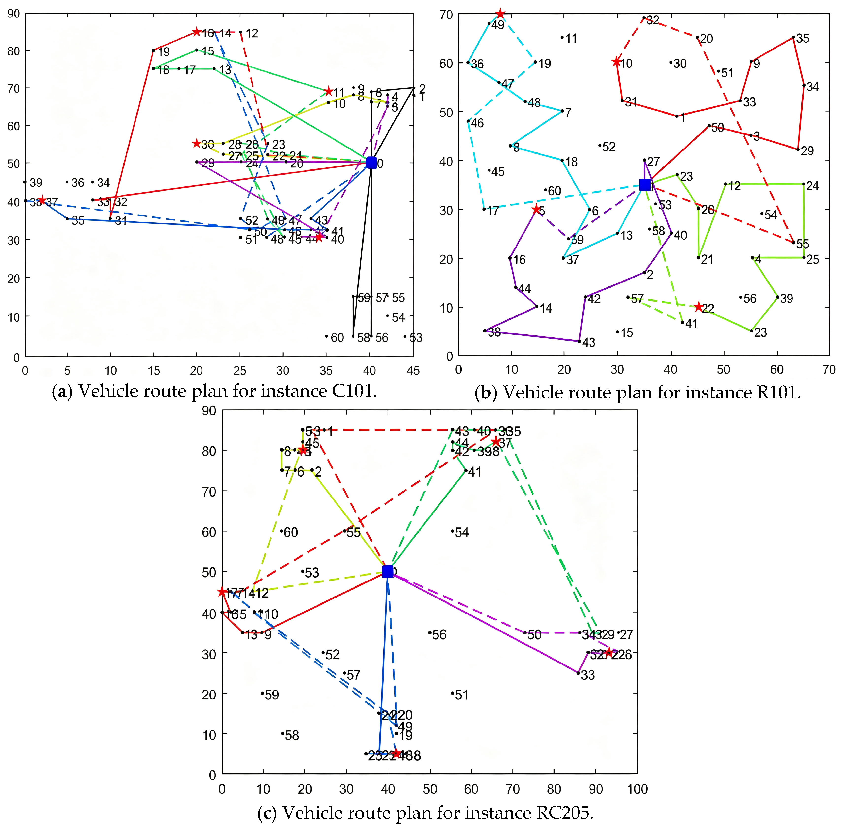
Figure 5 illustrates the route plans for instances C101, R201, and RC205. In the figure, the blue solid square denotes the distribution center, solid lines represent the routes in the pre-optimization stage, and dashed lines represent the routes in the dynamic optimization stage. The red pentagram marks the location where a vehicle stops when a dynamic update occurs, whereas nodes not traversed by any route indicate customers whose orders have been canceled. The figure shows that logistics route planning is closely associated with both the timing of dynamic updates and the spatial distribution of customer locations.

5.2.3. Case Simulation Under Different Optimization Objectives

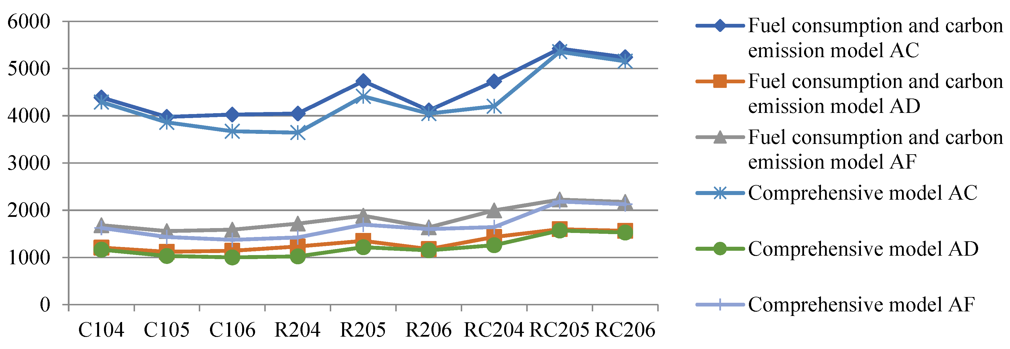
To validate the effectiveness of the proposed model, an alternative model with fuel consumption cost and carbon emission cost as the optimization objective is formulated and solved using the HABC-STA algorithm. Its results are then compared with those of the proposed comprehensive distribution cost model, as shown in Figure 6. The results indicate that the model focusing solely on fuel consumption and carbon emission costs produces higher total cost, higher fuel consumption cost, and higher travel cost than the proposed model. In particular, for the C-, R- and RC-type instances, the comprehensive distribution cost model reduces total cost by up to 8.77%, 9.94%, and 11.18%, respectively. At the same time, fuel consumption and carbon emission costs are reduced by up to 13.55%, 17.05% and 17.70%, respectively. This result can be attributed to the fact that the comprehensive distribution cost model evaluates the entire route in an integrated manner, balancing economic cost reduction with effective control of fuel consumption and carbon emissions, and thus achieves the objective of minimizing total cost. Therefore, the proposed model is capable of reducing fuel consumption and carbon emissions while also achieving the lowest total cost.

5.2.4. Comparative Analysis of Different Solution Algorithms

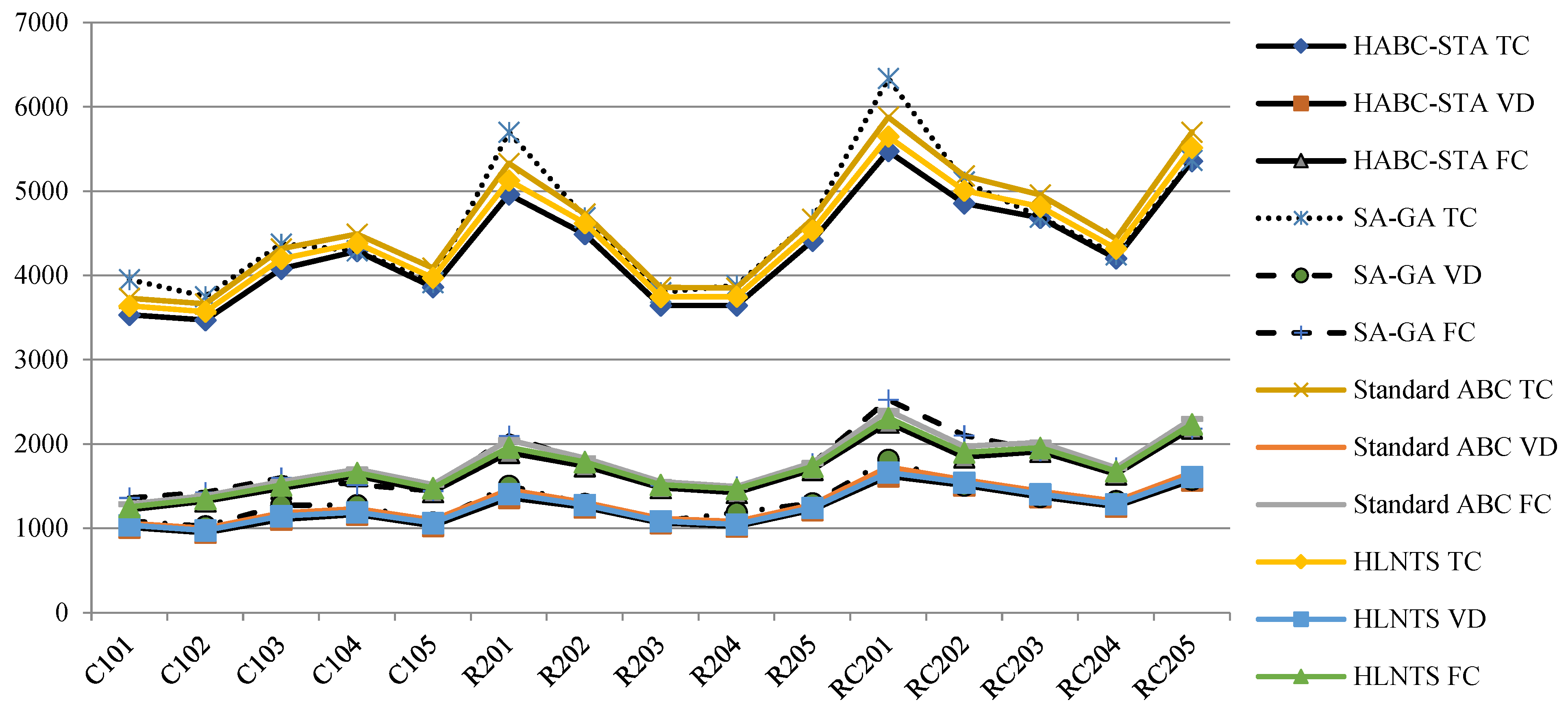
To compare the solution performance of different algorithms, a savings algorithm-genetic algorithm (SA-GA), standard ABC and hybrid large neighborhood Tabu search algorithm (HLNTS) are employed to solve the DDGVRPSTW model. Specifically, the savings algorithm is first used to generate the initial population for the genetic algorithm, which is then applied to obtain the pre-optimization routes. Subsequently, the remaining routes are updated according to the dynamic update strategy. Standard ABC retains the employed bee, onlooker bee and scout bee phases. HLNTS combines route removal, customer reinsertion, local route improvement and Tabu-based cycling control. The comparative results of the proposed HABC-STA algorithm and the other algorithms are presented in Figure 7.
The experimental results indicate that the average total distribution costs obtained by the HABC-STA algorithm for the C-, R- and RC-type cases are 19,233.21, 21,150.51, and 24,571.21, respectively. For the clustered C101-C105 instances, the HABC-STA algorithm reduces total distribution cost by up to 11.83% relative to the SA-GA algorithm, while saving as many as two vehicles. For the randomly distributed R201-R205 instances, the total distribution cost is reduced by up to 14.93%. In particular, for instance R203, the total distribution cost decreases by 4.23%, and up to four vehicles are saved. For the uniformly distributed RC201-RC205 instances, the HABC-STA algorithm reduces total distribution cost by up to 15.82% compared with the SA-GA algorithm, while saving as many as four vehicles. These findings suggest that the HABC-STA algorithm is particularly advantageous for logistics distribution problems with mixed dispersed and clustered customer distributions, followed by randomly distributed and highly concentrated customer logistics scenarios.
Compared with standard ABC, HABC-STA reduces the total distribution cost for the C-, R- and RC-type cases. For the C103 case, HABC-STA achieved the highest improvement of 5.52% compared to standard ABC. HABC-STA typically achieved the highest improvement of 6.90% compared to standard ABC among R cases. HABC-STA achieved the highest improvement of 6.89% compared to standard ABC among RC cases. This result indicates that the state-transition operators improve the search capability of the artificial bee colony framework. The improvement is most evident for the RC-type cases, which combine random and clustered customer distributions and therefore generate a more complex routing structure. Compared with HLNTS, HABC-STA achieves average cost reductions of 2.65%, 2.88%, and 2.90% for the C-, R- and RC-type cases, respectively. Although HLNTS obtains competitive solutions through large-neighborhood destruction and reconstruction, HABC-STA provides a lower average cost under the tested dynamic-demand and soft time window settings.

5.2.5. Ablation Experiments

To investigate the contribution of the state-transition operators, an ablation experiment is conducted by comparing HABC-STA with standard ABC. Standard ABC retains the standard employed bee, onlooker bee, and scout bee phases but removes all state-transition operators. The two algorithms use the same initialization procedure, population size, maximum number of iterations, objective function, constraint-handling mechanism, dynamic update strategy and random seed set.
The results are presented in Table 4. HABC-STA achieves lower mean total distribution costs than standard ABC for all three types of customer distributions. For the C, R and RC-type instances, the average cost reductions are 5.19%, 5.75%, and 6.06%, respectively. The largest improvement is observed for the RC-type instances, where customer locations exhibit both dispersed and clustered characteristics.
The comparison demonstrates that the state-transition operators contribute positively to the search performance of the proposed algorithm. In particular, the swap, shift, and reversal operators in the pre-optimization stage improve the local rearrangement of customer sequences, whereas the inter-route and intra-route operators in the dynamic stage provide additional flexibility for adjusting routes after demand changes occur. The lower standard deviations obtained by HABC-STA also indicate that the proposed hybrid search mechanism improves solution stability.
For the statistical analysis, a paired two-sided Wilcoxon signed-rank test is performed using the mean total cost of each benchmark instance. The mean total cost obtained from each instance is treated as one paired observation, so that each benchmark instance contributed equally to the comparison. The results are shown in Table 5. The comparison between HABC-STA and standard ABC gives a Holm-adjusted p-value of 0.003, while the comparison between HABC-STA and SA-GA also gives a Holm-adjusted p-value of 0.003. The comparison between HABC-STA and HLNTS yields a smaller Holm-adjusted p-value of 1.831 × 10⁻⁴. All adjusted p-values are below the significance level of 0.05, which indicates that the observed improvements of HABC-STA are statistically significant under the tested instances.

5.2.6. Computation Time Analysis

To assess the practical deployment capability of the algorithm, this paper further calculates the computation time in two solving phases. The computation time for the pre-optimization phase is defined as the time from the generation of the initial population to the acquisition of the pre-optimized path. The computation time for the dynamic re-optimization stage is defined as the time from the dynamic moment T that triggers the re-optimization until the output of an updated path that satisfies vehicle capacity constraints, customer service constraints and path continuity constraints. Computation time of HABC-STA algorithm on various customer scales is shown in Table 6. Each instance is repeatedly run 15 times with different random seeds. The computation time of average and maximum values are recorded. The experiments are conducted in the same hardware and software environment, and the timing does not include data reading, result output and plotting time.
The results show that the computational time increases with the number of customers, as the search space and the number of route combinations become larger. Nevertheless, the dynamic re-optimization stage requires substantially less time than the pre-optimization stage because it only optimizes the remaining unserved customers based on the current vehicle states. In particular, the maximum dynamic re-optimization time for the 100-customer instance is 6.9 s, which indicates that the proposed method has potential for online route adjustment in dynamic logistics.

5.2.7. Simulation Analysis of a Real-World Case

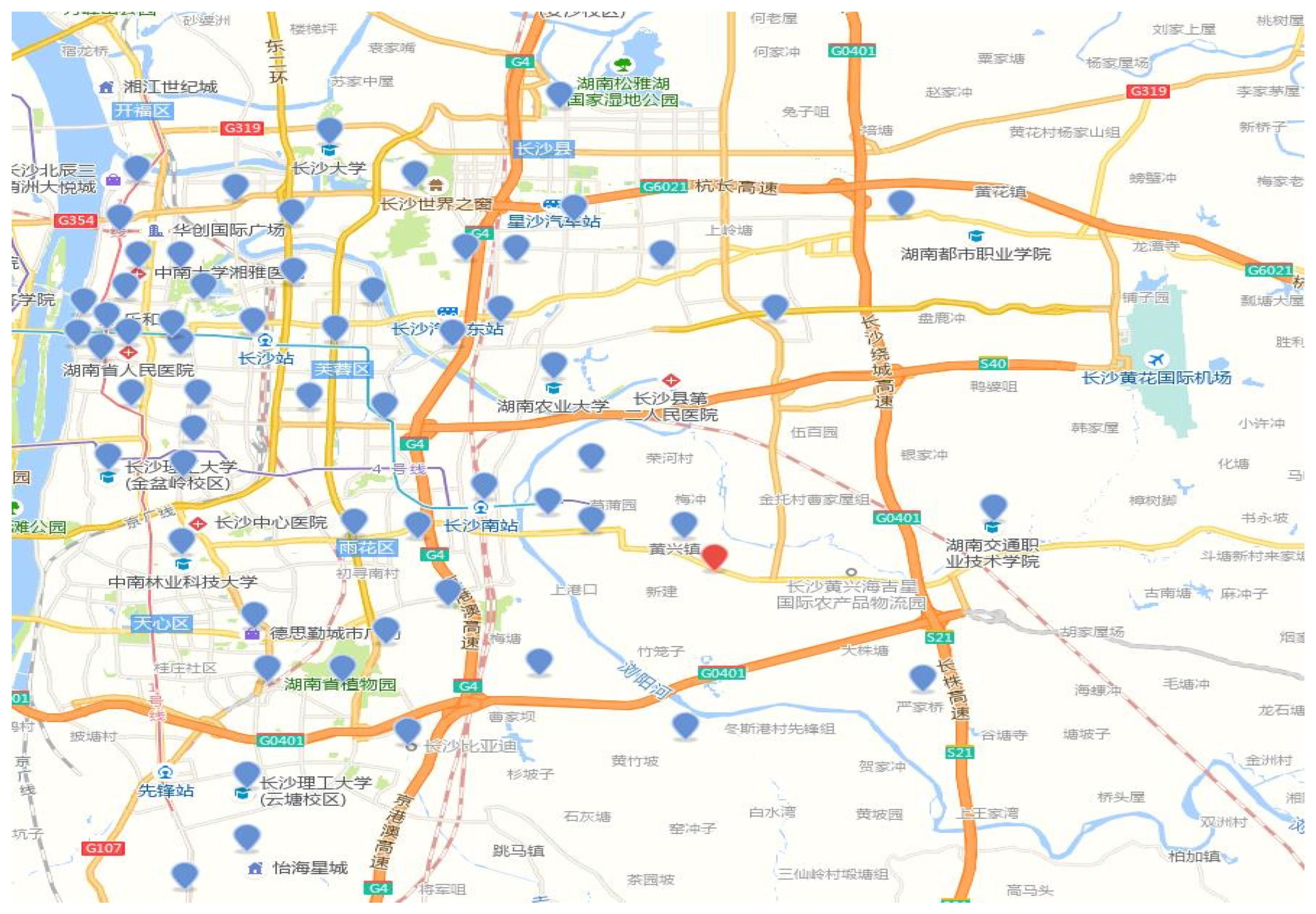
A real-world case from a logistics distribution enterprise in Changsha, Hunan Province, is used for further validation. Considering the diversity and complexity of actual distribution operations, 60 customer nodes are randomly selected within the service area. Their spatial distribution is shown in Figure 8, and their demand quantities and time windows vary across customers. The maximum vehicle capacity is set to 200. The longitude and latitude of the distribution center are (113.120656, 28.127722). Using ArcGIS Pro 3.2, the locations of all customer nodes were transformed into a planar coordinate system, in which the distribution center is located at (15,372, 10,414). To examine the effect of dynamic demand at different update times on the routing plan, the dynamic update factor is fixed as the addition of 10 new customer nodes. To ensure the reliability of the results, each experiment is repeated 20 times and the average values are reported. As shown in Table 7, within a certain time range, the total cost increases as the dynamic update time becomes later, reaching a maximum of 3098.04 when T = 200. The reason may be that the distribution of customer locations and demands in actual cases is random, leading to an increase in costs during the first stage. However, the fixed cost in the two stages remains unchanged, indicating that the dynamic update time does not affect the number of vehicles dispatched from the distribution center in each stage. Meanwhile, as the dynamic update time increases, the number of vehicles used in the second stage decreases.

6. Conclusions

This study addressed the dynamic-demand green vehicle routing problem with soft time windows by developing a two-stage optimization model aimed at minimizing the sum of travel cost, fuel consumption cost, carbon emission cost, penalty cost, and fixed dispatch cost. A hybrid artificial bee colony state-transition algorithm (HABC-STA) was proposed to solve the model, and its performance was evaluated using Solomon benchmark instances and a real-world case. The results indicate that the timing of dynamic updates plays an important role in cost control. Within a certain time range, a later dynamic update often leads to a lower total distribution cost. However, the cost will increase in real case distribution, which implies that the effect of update timing is instance dependent. In addition, the routing scheme based on minimizing comprehensive distribution cost not only reduces fuel consumption and carbon emissions, but also achieves the lowest total cost. The proposed HABC-STA algorithm further demonstrates strong effectiveness in reducing comprehensive distribution cost, especially in terms of fuel consumption and carbon emission cost. Nevertheless, this study assumes a constant vehicle speed in order to simplify the model. In real distribution environments, traffic congestion and changing road conditions may significantly affect vehicle speed and distribution cost. Future research will therefore incorporate real-time traffic data to examine the impact of congestion and road condition variations on logistics distribution and to further optimize routing and scheduling decisions through dynamic adjustment strategies. Also, an important research direction is to extend the proposed framework to address more complex dynamic events, including real-world dynamic logistics systems characterized by demand updates, customer cancellations, and changes in time windows.

Author Contributions

Conceptualization, K.Z. and X.Z.; Methodology, M.H., K.Z., Q.W. and L.S.; Software, M.H., Q.W. and L.S.; Validation, M.H., Q.W. and L.S.; Formal analysis, Q.W. and L.S.; Investigation, M.H. and L.S.; Resources, K.Z. and X.Z.; Data curation, K.Z. and Q.W.; Writing—original draft, K.Z.; Writing—review & editing, X.Z.; Visualization, L.S.; Supervision, K.Z., Q.W. and X.Z.; Project administration, K.Z.; Funding acquisition, X.Z. All authors have read and agreed to the published version of the manuscript.

Funding

This research was supported by the Key Project of Xiangjiang Laboratory (25XJ02003).

Institutional Review Board Statement

This study did not involve human participants, human data, animals, or any material requiring ethical approval. Therefore, ethical approval and informed consent were not applicable.

Data Availability Statement

Data shall be made available upon request. The source code used in this study is publicly available upon request.

Acknowledgments

The authors would like to thank the editor and anonymous reviewers for their constructive comments and valuable suggestions, which helped improve the quality of this manuscript.

Conflicts of Interest

The authors declare no conflicts of interest.

References

  1. AbdAllah, A.M.F.M.; Essam, D.L.; Sarker, R.A. On solving periodic re-optimization dynamic vehicle routing problems. Appl. Soft Comput. 2017, 55, 1–12. [Google Scholar] [CrossRef] [Scilit]
  2. Ulmer, M.W.; Soeffker, N.; Mattfeld, D.C. Value function approximation for dynamic multi-period vehicle routing. Eur. J. Oper. Res. 2018, 269, 883–899. [Google Scholar] [CrossRef] [Scilit]
  3. Pillac, V.; Guéret, C.; Medaglia, A.L. An event-driven optimization framework for dynamic vehicle routing. Decis. Support Syst. 2012, 54, 414–423. [Google Scholar] [CrossRef] [Scilit]
  4. Li, Y.; Fan, H.M.; Zhang, X.N. Periodic optimization model and solution method for the vehicle routing problem under dynamic demand. Chin. J. Manag. Sci. 2022, 30, 254–266. [Google Scholar]
  5. Li, Y.F.; Gao, Z.Y.; Li, J. Research on the vehicle routing problem in dynamic networks. J. Manag. Sci. China 2014, 17, 1–9. [Google Scholar]
  6. Wang, F.; Liao, F.; Li, Y.; Yan, X.; Chen, X. An ensemble learning based multi-objective evolutionary algorithm for the dynamic vehicle routing problem with time windows. Comput. Ind. Eng. 2021, 154, 107131. [Google Scholar] [CrossRef] [Scilit]
  7. Erdoğan, S.; Miller-Hooks, E. A green vehicle routing problem. Transp. Res. Part E Logist. Transp. Rev. 2012, 48, 100–114. [Google Scholar] [CrossRef] [Scilit]
  8. Liu, C.S.; Shen, L.Z.; Sheng, H.Y.; Lv, X.Y.; Qu, Y.P. Research on the low-carbon time-dependent vehicle routing problem considering traffic congestion avoidance. Control Decis. 2020, 35, 2486–2496. [Google Scholar]
  9. Çimen, M.; Soysal, M. Time-dependent green vehicle routing problem with stochastic vehicle speeds: An approximate dynamic programming algorithm. Transp. Res. Part D Transp. Environ. 2017, 54, 82–98. [Google Scholar] [CrossRef] [Scilit]
  10. Andelmin, J.; Bartolini, E. An exact algorithm for the green vehicle routing problem. Transp. Sci. 2017, 51, 1288–1303. [Google Scholar] [CrossRef] [Scilit]
  11. Yao, K.; Yang, B.; Zhu, X.L. Low-carbon vehicle routing optimization considering time-dependent traffic conditions. Comput. Eng. Appl. 2019, 55, 231–237. [Google Scholar]
  12. Liu, C.S.; Zhou, X.C.; Sheng, H.Y.; Luo, L. Research on the time-dependent vehicle routing problem with time windows for fresh e-commerce distribution: A perspective balancing economic and environmental costs. Control Decis. 2020, 35, 1273–1280. [Google Scholar]
  13. Zhao, Z.X.; Li, X.M.; Zhou, X.C. Optimization of the multi-vehicle-type green vehicle routing problem considering congestion zones. J. Comput. Appl. 2020, 40, 883–890. [Google Scholar]
  14. Zhou, X.C.; Liu, C.S.; Zhou, K.J.; He, C.H.; Huang, X.B. Time-dependent green vehicle routing model and improved ant colony algorithm. J. Manag. Sci. China 2019, 22, 57–68. [Google Scholar]
  15. Jia, Y.J.; Ding, H.N.; Li, J.; Yang, D. Electric vehicle routing problem considering time-varying speed and dynamic demand. Ind. Eng. Manag. 2022, 27, 59–66. [Google Scholar]
  16. Ge, X.L.; Zhu, Z.Q.; Jin, Y.Z. Dynamic electric vehicle routing optimization based on a two-stage solution strategy. Oper. Res. Manag. Sci. 2022, 31, 57–63. [Google Scholar]
  17. Du, Q.; Nan, L.J.; Chen, Y.R. Electric vehicle routing problem with dynamic demand in context of crowdsourcing. Comput. Integr. Manuf. Syst. 2024, 30, 2588–2607. [Google Scholar]
  18. Guo, D.; Wang, J.; Zhao, J.B.; Sun, F.; Gao, S.; Li, C.D.; Li, M.H.; Li, C.C. A vehicle path planning method based on a dynamic traffic network that considers fuel consumption and emissions. Sci. Total Environ. 2019, 663, 935–943. [Google Scholar] [CrossRef] [Scilit] [PubMed]
  19. Km, S.; Pitam, S.; Shubhankar, K. Dynamic adaptive large neighborhood search approach for the uncertain multi-objective green vehicle routing problem. Appl. Soft Comput. 2026, 199, 115323. [Google Scholar] [CrossRef] [Scilit]
  20. Nan, L.J.; Chen, Y.R.; Zhang, Z.C. An improved adaptive large neighborhood search algorithm for the mixed vehicle routing problem with dynamic demand. Appl. Res. Comput. 2021, 38, 2926–2934. [Google Scholar]
  21. Reza, A.F.; Javad, R.; Iraj, M. Green vehicle routing and scheduling problem with heterogeneous fleet including reverse logistics in the form of collecting returned goods. Appl. Soft Comput. 2020, 94, 106462. [Google Scholar] [CrossRef] [Scilit]
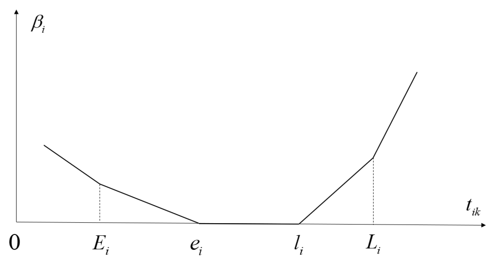
Figure 1. Piecewise linear penalty cost function of time windows.
Electronics 15 03780 g001
Figure 2. Swap operation.
Electronics 15 03780 g002
Figure 3. Shift operator.
Electronics 15 03780 g003
Figure 4. Symmetry operator.
Electronics 15 03780 g004
Figure 5. Vehicle routing diagram for the simulation instance.
Electronics 15 03780 g005
Figure 6. Solution results of instances for different optimization objective models.
Electronics 15 03780 g006
Figure 7. Comparison results of various algorithms.
Electronics 15 03780 g007
Figure 8. Distribution of actual customer locations.
Electronics 15 03780 g008
Table 1. The meaning of notation and variables.
SymbolDescription
0origin depot
r + 1destination depot
Hcustomer set, H = {1, …, h}
Kset of delivery vehicles K = 1, 2, …, k.
U1set of the origin depot and customer nodes, U1 = {0} ∪ H
U2set of the destination depot and customer nodes, U2 = {r + 1} ∪ H
Bmaximum capacity of a delivery vehicle
bijkload carried by vehicle k on arc (i,j)
qidemand of customer i
dijdistance between nodes i and j
[ei, li]preferred time window of customer i
[e0, lr+1]service time window of the depot
[Ei, li]acceptable time window of customer i
vaverage travel speed of vehicles
tikarrival time of vehicle k at node i
tijktravel time of vehicle k on arc (i,j)
stijkservice time of vehicle k at customer i
c 1 fixed dispatch cost per vehicle (CNY/vehicle)
c 2 unit travel cost (CNY/km)
c 3 unit fuel cost (CNY/L)
c 4 unit carbon emission cost (CNY/kg)
βipenalty coefficient for different time intervals
pitime window penalty cost
fijkfuel consumption rate of vehicle k on arc (i,j)
eijkcarbon emission rate of vehicle k on arc (i,j)
xijkbinary variable equal to 1 if vehicle k travels on arc (i,j), and 0 otherwise
yikbinary variable equal to 1 if customer i is served by vehicle k, and 0 otherwise
Mset of newly added delivery vehicles M = k + 1 , k + 2 , , k + m
Rset of all delivery vehicles R = 1 , 2 , , k , k + 1 , k + 2 , , k + m
Ftotal number of unserved customers from the first stage and newly added customers
Aset of virtual nodes
A1set of virtual nodes under the periodic update strategy
A2set of virtual nodes under the dynamic event update strategy
A3set of virtual nodes under the customer-node update strategy
N 1 set of customer nodes and virtual nodes N 1 = F A
N 2 set of customer nodes and the destination depot N 2 = F { r + 1 }
N 3 set of the origin depot, virtual nodes, and customer nodes N 3 = { 0 } A F
N 4 set of virtual nodes, customer nodes, and the destination depot N 4 = A F { r + 1 }
Nset of all nodes
b s k remaining load of vehicle k after the first stage
Z 0 i cost from the origin depot to virtual node i at the end of the first stage
Table 2. Simulation results at different dynamic moments.
TACAC1AD1AG1AP1AF1
803890.871647.59241.401000104.78301.40
1004534.141852.26266.311000250.54335.40
1204388.752040.28294.391000372.77373.12
1403711.992289.02312.991000577.87398.16
TAD2AG2AP2AF2CN1CN2
80818.280400.851024.1455
100869.90200526.071085.9056
120758.85200495.40894.2156
140423.75200315.00484.2156
Table 3. Simulation results for different customer distributions.
InstanceTACAC1/AC2AD1/AD2AG1/AG2AP1/AP2AF1/AF2CN1/CN2
C1015003476.891624.53237.821000.0087.03299.665
1852.36469.45200.00592.78590.136
C1055003348.011724.95300.671000.0046.49377.785
1623.06414.60200.00468.91539.556
C2015006143.373372.38325.671000.001384.57662.135
2770.99504.080.001636.04630.874
C2055006385.682871.84244.421000.001063.30564.125
3513.84462.800.002470.87580.174
C2065005523.742559.85276.591000.00768.85514.405
2963.89427.700.002000.34535.854
R1012002199.121922.75394.91800.00230.38497.444
276.37123.560.000.00152.814
R1052002762.981959.12419.45800.00209.84529.824
803.86252.21200.0028.10323.555
R2012003184.002661.00422.09800.00905.67533.244
523.00194.040.0088.90240.064
R2052003167.692568.46453.38800.00679.52635.564
599.23207.750.00133.46258.023
R2062002279.832259.74431.86800.00425.02602.864
520.09151.360.00181.20187.533
RC1011003072.261647.09257.451000.0063.82325.825
1425.17597.740.0083.30744.135
RC1051003360.371615.54260.431000.0027.45327.665
1744.83733.930.0092.88918.025
RC2011003638.042152.60264.601000.00554.37333.635
1485.44506.970.00347.12631.355
RC2051003564.362494.35346.891000.00705.34442.125
1070.01340.52200.0084.09445.406
RC2061003397.372710.52380.651000.00773.15556.725
686.85283.550.0051.71351.594
Table 4. Ablation results of HABC-STA and standard ABC.
Instance TypeHABC-STA Mean ± SDStandard ABC Mean ± SDImprovement(%)
C-type19,233.21 ± 286.4420,285.94 ± 321.555.19
R-type21,150.51 ± 314.6222,439.83 ± 338.105.75
RC-type24,571.21 ± 402.1826,157.16 ± 436.726.06
Table 5. Wilcoxon signed-rank test results.
ComparisonW Statisticp-ValueHolm-Adjusted p-Value
HABC-STA vs. Standard ABC12.00.0010.003
HABC-STA vs. SA-GA8.00.0010.003
HABC-STA vs. HLNTS06.104 × 10−51.831 × 10⁻⁴
Table 6. Computation time of HABC-STA algorithm on various customer scales.
Number of CustomersPre-Optimization Time (s)Average Dynamic Re-Optimization Time (s)Maximum Dynamic Re-Optimization Time (s)
6014.81.62.4
8031.52.84.1
10058.94.66.9
Table 7. Computational results at different dynamic moments.
TACAC1AD1AG1AP1AF1
1002426.291626.92157.891000.00461.667.37
1202781.972013.79199.941000.00585.67228.18
1402928.692303.57216.021000.00683.36404.19
1603082.112462.91223.171000.00693.87545.87
1803097.022490.01244.071000.00691.63554.31
2003098.042490.45242.021000.00718.04530.39
TAD2AG2AP2AF2CN1CN2
100199.36400.00189.7210.2857
120180.12400.00178.999.0755
14081.98400.00139.114.0254
16088.78400.00126.394.0253
18083.00400.00119.984.0353
20082.42400.00121.213.9653
Disclaimer/Publisher’s Note: The statements, opinions and data contained in all publications are solely those of the individual author(s) and contributor(s) and not of MDPI and/or the editor(s). MDPI and/or the editor(s) disclaim responsibility for any injury to people or property resulting from any ideas, methods, instructions or products referred to in the content.