An Improved Q-Learning-Based AODV Routing Protocol for Marine Cross-Medium Acoustic–Radio Collaborative Networks

Abstract

Marine cross-medium acoustic–radio collaborative networks must route traffic across heterogeneous underwater acoustic and radio links while coping with energy imbalance, congestion, and mobility-induced link instability. This paper proposes Q-Learning AODV, an AODV extension that integrates distributed Q-value updating and multipath route maintenance into existing RREQ, RREP, and HELLO procedures. The routing reward combines normalized residual energy, queue availability, inter-node distance/link stability, relative velocity, and, for air–sea links, elevation-angle information. The protocol maintains multiple node-disjoint candidate paths and forwards data through the currently highest-valued path. NS-3 simulations are reported for underwater-to-underwater, underwater-to-air, and air-to-underwater communication scenarios. Relative to conventional AODV, Q-Learning AODV increases packet delivery ratio from 55.8% to 88.3%, from 68.3% to 76.1%, and from 86.9% to 91.9%, corresponding to relative improvements of 58.2%, 11.4%, and 5.8%, respectively. The results indicate improved delivery reliability and communication-subsystem energy balancing at the cost of additional state exchange, Q-table storage, and route-selection computation.

1. Introduction

Marine observation, resource exploration, emergency response, and autonomous operations increasingly require end-to-end information exchange among underwater nodes, surface gateways, aerial platforms, and shore-based systems. Marine cross-medium acoustic–radio collaborative networks use surface buoys or other gateways to interconnect underwater acoustic subnetworks with radio networks, providing an important communication substrate for three-dimensional marine Internet of Things applications [1,2,3]. Routing performance directly affects packet delivery ratio (PDR), end-to-end delay, throughput, and the operational lifetime of energy-constrained relay nodes [4,5].

The routing problem is difficult because the two media have markedly different characteristics. Underwater acoustic links exhibit low propagation speed, limited bandwidth, long delay, and strong environmental variability [6,7], whereas radio links provide higher rates but are still affected by mobility, geometry, and sea-surface propagation. Conventional radio protocols such as Ad hoc On-Demand Distance Vector (AODV), Dynamic Source Routing (DSR), and Optimized Link State Routing (OLSR) [8,9,10] do not explicitly account for these heterogeneous link properties. Conversely, representative underwater protocols such as Vector-Based Forwarding (VBF), Depth-Based Routing (DBR), and Channel-Aware Routing Protocol (CARP) [11,12,13] are designed primarily for acoustic subnetworks and cannot be transferred directly to heterogeneous cross-medium routing without additional adaptation [14,15].

Three coupled problems motivate this study. First, gateway and relay traffic can concentrate energy expenditure on a small number of nodes. Second, acoustic bottlenecks can accumulate queues and create congestion. Third, node mobility and heterogeneous propagation conditions make previously selected paths unstable. Reinforcement learning provides a mechanism for adapting forwarding preferences from online observations rather than relying on one fixed routing metric [16,17]; however, existing learning-based underwater routing methods remain predominantly single-medium and often optimize only a subset of energy, congestion, mobility, and link-stability objectives.

Accordingly, this study is organized around three research questions: RQ1: How can Q-Learning be integrated into AODV route discovery and maintenance without introducing a new control-packet type? RQ2: How can locally obtainable energy, queue, geometric, and mobility information be combined into a normalized reward for heterogeneous acoustic–radio links? RQ3: Can Q-value-driven maintenance of multiple candidate paths improve delivery reliability and communication-subsystem lifetime under different cross-medium scenarios and mobility conditions?

To answer these questions, this paper proposes Q-Learning AODV. The technical contributions are as follows. (1) Existing RREQ, RREP, and HELLO procedures are extended to carry routing-state fields required for distributed Q-value updates; this reuses existing control-packet types, although it increases their payload size. (2) A normalized multi-objective reward combines residual energy, queue availability, distance-based link stability, relative velocity, and link-type-dependent elevation information. (3) Multiple node-disjoint candidate paths are maintained for a destination and ranked using continuously updated Q-values, so that data forwarding can switch to a better available path when network conditions change. (4) The implementation and evaluation explicitly distinguish algorithmic benefits from the additional communication, computation, and storage overhead introduced by learning and multipath maintenance.

The remainder of this paper is organized as follows. A separate Section 2 reviews routing and reinforcement-learning studies and identifies the gap addressed by this work. Section 3 presents the cross-medium network and propagation models. Section 4 describes the Q-Learning AODV protocol, including the Markov decision process (MDP), reward design, state acquisition, protocol workflow, and complexity. Section 5 reports the simulation methodology and results. Section 6 concludes the paper and discusses limitations and future work.

2. Related Work

Q-Learning has been widely studied for adaptive routing in underwater acoustic sensor networks. Hu et al. [18] proposed QELAR, which incorporates residual energy and neighborhood energy information to extend network lifetime. Jin et al. [19] proposed a Q-Learning delay-aware routing algorithm that considers delay cost and network lifetime. RCAR [20] combines reinforcement learning with congestion and energy awareness, whereas EDORQ [21] integrates Q-Learning with depth-constrained opportunistic forwarding. These approaches demonstrate the usefulness of online value updating, but their objectives and signaling assumptions are mainly designed for underwater acoustic networks.

Routing stability and service adaptability have also been incorporated into Q-Learning designs. Zhou et al. [22] proposed a Q-Learning-based anypath routing method with candidate forwarding priorities and holding-time control. Chen et al. [23] investigated Q-Learning-based multi-hop cooperative routing, and Nandyala et al. [24] proposed topology-aware candidate filtering followed by Q-Learning selection. Zhang et al. [25] considered service-aware multi-factor rewards, while Li et al. [26] incorporated link-aware information into Q-Learning-based underwater routing. More recently, energy-aware deep reinforcement learning has also been used for resource-constrained underwater acoustic systems, illustrating the broader value of adaptive learning under energy limitations [27].

A separate body of work has considered cross-medium networking. Lyu et al. [15] studied optimized AODV routing for cross-medium acoustic–radio collaborative networks, showing that medium-aware route discovery, link-stability assessment, and control-overhead reduction are important when conventional ad hoc routing is extended across heterogeneous marine links. Nevertheless, the combination of cross-medium AODV control, distributed Q-value updating, queue/energy awareness, mobility information, and multipath maintenance remains insufficiently studied. Practical feasibility is also important: learning variables must be obtained by identifiable network entities and exchanged with bounded overhead rather than assumed to be available from an omniscient environment [28].

Table 1. Comparison with representative learning-based routing schemes.

Method	State/Decision Information	Reward/Objective Emphasis	Routing Strategy	Mobility Consideration	Communication Medium
QELAR [18]	Residual and neighborhood energy	Energy balancing and lifetime	Q-Learning next-hop selection	Limited	Underwater acoustic
QDAR [19]	Delay and neighbor state	Delay/lifetime trade-off	Q-Learning routing	Indirect	Underwater acoustic
RCAR [20]	Congestion and energy	Congestion avoidance and energy	RL-based adaptive routing	Limited	Underwater acoustic
QLFR [22]	Candidate-link/Q information	Reliability and delay	Q-Learning anypath/candidate forwarding	Considered through dynamic candidates	Underwater acoustic
QTAR [24]	Topology and Q information	Energy efficiency and stability	Topology filtering + Q-Learning	Topology-aware	Underwater acoustic
SAQR [25]	Multi-factor service state	Service-aware multi-objective reward	Q-Learning routing	Limited	Underwater acoustic
Q-Learning AODV (this work)	Residual energy, queue availability, position/distance, velocity, link type, Q-value	Energy, congestion, geometric/link stability, mobility	AODV control + Q- value-ranked node-disjoint paths	Explicit relative- velocity term	Acoustic–radio cross-medium

summarizes the main differences between representative learning-based routing studies and the present work. The comparison is intentionally limited to dimensions directly relevant to this manuscript.

The above literature reveals three gaps that motivate this study. First, most Q-Learning routing schemes are evaluated in a single acoustic medium rather than a heterogeneous acoustic–radio network. Second, energy, congestion, mobility, and cross-medium geometry are rarely integrated within one lightweight distributed routing decision. Third, many reinforcement-learning formulations do not explicitly explain where each observation is obtained or what signaling is needed to distribute it. The proposed method therefore focuses on a cross-medium, locally observable formulation coupled to existing AODV control procedures, while also making its additional overhead and modeling limitations explicit.

3. Acoustic–Radio Collaborative Network Model and Overview

3.1. Overview and Architecture of the Acoustic–Radio Collaborative Network

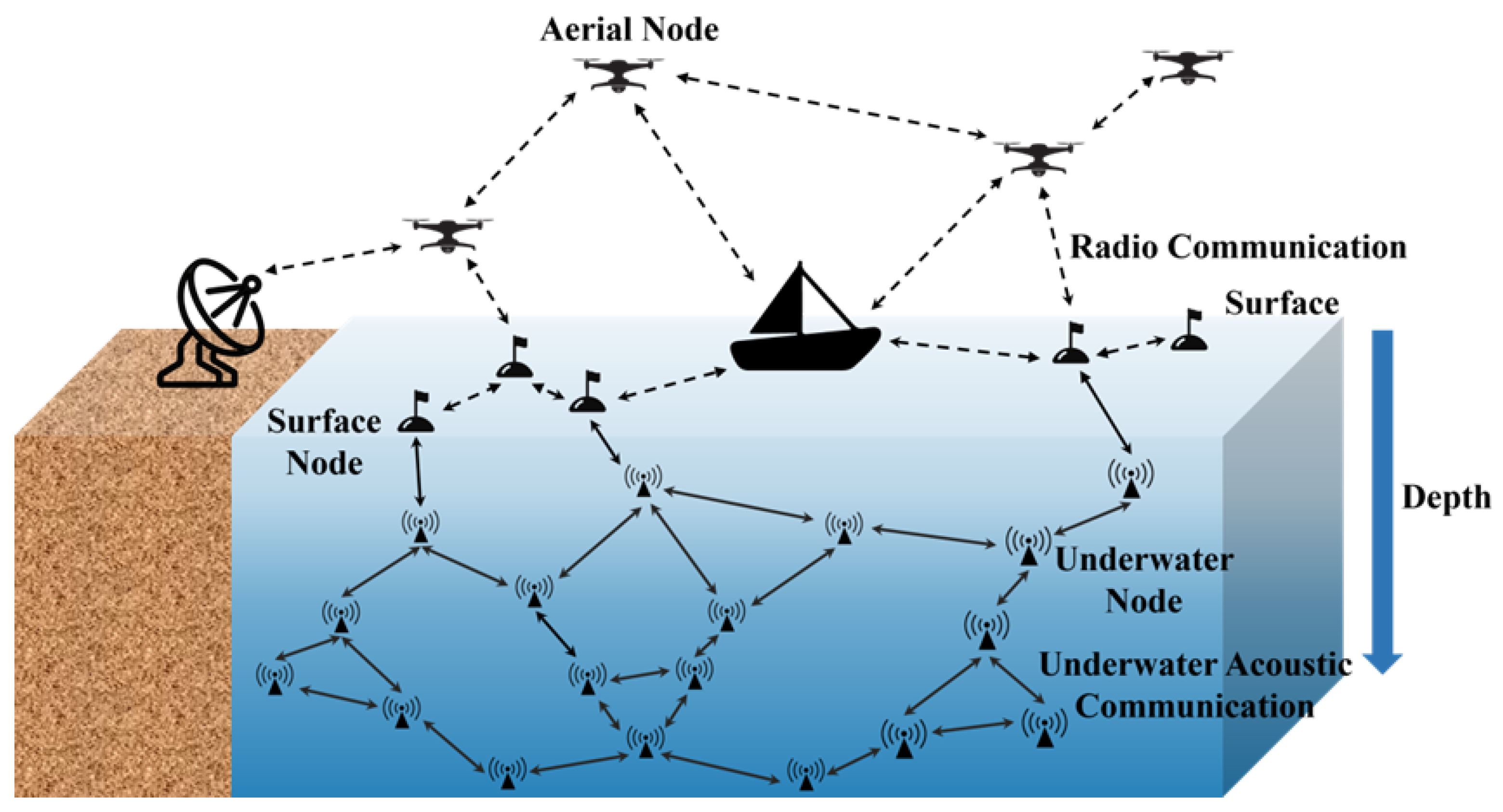
As shown in Figure 1, the acoustic–radio collaborative network is characterized by layered deployment and heterogeneous links in its overall architecture. The underwater layer consists of network nodes responsible for environmental sensing and detection tasks, including both mobile platforms with a certain degree of autonomous maneuverability and fixed observation nodes permanently deployed in the target sea area. Information exchange among underwater nodes relies on underwater acoustic communication links, whose performance is significantly constrained by low propagation speed, limited available bandwidth, and time-varying channel conditions. Surface-layer nodes play a key role in information relaying and cross-medium collaboration within the network. On the one hand, they achieve relatively high-speed and low-latency data transmission through radio links; on the other hand, by integrating underwater acoustic communication modules, they maintain connectivity with the underwater network and accomplish cross-medium data access, signal conversion, and forwarding. Therefore, they typically serve as core nodes for data aggregation and heterogeneous communication coordination. The aerial layer introduces radio communication nodes represented by unmanned aerial vehicles, which can further expand network coverage and enhance system flexibility. By establishing radio links with surface nodes, aerial nodes support large-scale information backhaul and temporary communication services.

Based on the above multi-layer heterogeneous node composition and diversified communication modes, this paper develops a network model integrated with a Q-Learning-based routing mechanism for acoustic–radio collaborative application scenarios. Different types of nodes and their corresponding communication links are uniformly abstracted and modeled, thereby establishing a simulation platform for routing protocol design and performance evaluation. Under a unified network topology, the proposed model can simultaneously capture the differences between underwater acoustic links and radio links in terms of propagation characteristics, delay characteristics, and communication reliability. This provides experimental support for the study of cross-medium routing mechanisms and ensures that the subsequent performance evaluation is conducted on a consistent modeling basis with reproducible simulations.

From the perspective of network operation, various nodes in the acoustic–radio collaborative network generally possess independent capabilities for data sensing, information transmission and reception, and distributed routing processing. In marine environments without fixed communication infrastructure, the network relies on cooperative interactions among nodes to accomplish data forwarding and route maintenance. Owing to environmental complexity and node mobility, the spatial distribution of nodes and link connectivity change continuously over time, resulting in a highly dynamic network topology. Although such networks share certain organizational similarities with mobile ad hoc networks, the coexistence of heterogeneous links, including underwater acoustic communication and radio communication, substantially increases the complexity of network control and routing decision making in cross-medium information transmission, making conventional routing strategies designed for single-medium networks difficult to apply directly. At the application level, information exchange among underwater nodes can be achieved either through multi-hop underwater acoustic communication or through cross-medium collaborative paths established via surface nodes for cooperation and data sharing. Data transmission between underwater nodes and surface nodes, however, depends on relay nodes equipped with both underwater acoustic and radio communication capabilities to perform signal conversion and forwarding, thereby supporting centralized return of observation data and bidirectional interaction between underwater systems and surface control platforms. Overall, the heterogeneity and dynamics of network structure, link characteristics, and operating mechanisms impose higher requirements on routing protocols in terms of path selection, adaptive adjustment, and resource coordination, while also providing the research basis for introducing intelligent routing methods with environmental awareness and self-learning capability.

3.2. Propagation Loss Modeling

Because acoustic–radio collaborative networks involve multiple transmission media in underwater and aerial environments, signal propagation characteristics vary significantly across different media. Therefore, dedicated propagation loss models must be established to accurately characterize the attenuation behavior of signals in each medium. In this study, the underwater propagation loss model and the over-sea propagation loss model are developed and analyzed as follows.

3.2.1. Underwater Propagation Loss Model

Underwater acoustic communication is adopted for underwater transmission in the acoustic–radio collaborative network. In this study, the Thorp underwater propagation loss model implemented in the NS-3 simulation platform is employed [29]. The acoustic attenuation is given by

$$10{\log }_{10}A\left(d_u,f_u\right)=k{\log }_{10}\left(d_m\right)+d_{km}a\left(f_u\right)$$

(1)

where $f_u$ denotes the signal frequency, $d_u$ is the point-to-point distance, and $A(d_u,f_u)$ represents the attenuation of the acoustic wave at distance d and frequency f, measured in decibels (dB). The term $k{\log }_{10}\left(d_m\right)$ denotes the loss caused by acoustic spreading, where k is the spreading factor. In practical transmission, $k=1$ corresponds to spherical spreading, whereas $k=2$ corresponds to cylindrical spreading. Here, $d_m$ is the propagation distance of the acoustic wave in meters, and $a\left(f_u\right)$ is the acoustic absorption coefficient. In addition, $d_{km}=d_m/1000$ is the transmission distance in kilometers. The absorption coefficient is calculated using the Thorp empirical formula [30].

3.2.2. Over-Sea Propagation Loss Model

In the acoustic–radio collaborative network, three propagation loss models are introduced to characterize radio propagation under different inter-node communication scenarios, namely the air-to-air propagation loss model, the air-to-sea propagation loss model, and the sea-surface-to-sea-surface propagation loss model.

The air-to-air propagation loss model is used to describe the radio link loss between unmanned aerial vehicle nodes. Since this type of link corresponds to point-to-point line-of-sight transmission between aerial nodes, the classical Friis propagation loss model is adopted for its characterization [31].

When the transmitting node is located in the air and the receiving node is a surface buoy, an air-to-sea link is formed. Its geometry depends on both horizontal separation and altitude difference. The elevation-angle LoS-probability expression in [32] was originally developed for terrestrial low-altitude-platform environments. In the present model it is used as a monotonic geometry-dependent LoS weighting function under an open, low-obstruction setting, rather than as a literal representation of building blockage or as a field-fitted maritime propagation law. The resulting radio-link conclusions are interpreted at this comparative modeling level. Let h denote the height difference between the aerial node and the surface buoy, and let r denote the horizontal distance. Then, the elevation angle between the two nodes can be expressed as:

$${\theta }_{AS}={\displaystyle \frac{180}{\pi }}\times \arctan \left({\displaystyle \frac{h}{r}}\right)$$

(2)

Furthermore, the LoS probability model is used to characterize the propagation properties of the air-to-sea link, which is given by:

$$P_{LoS}={\displaystyle \frac{1}{1+a\exp \left[-b\left({\theta }_{AS}-a\right)\right]}},$$

(3)

where $P_{LoS}$ denotes the probability of LoS propagation between the surface buoy and the aerial node. The parameters a and b are environment-dependent constants. In this study, the low-obstruction parameter setting from [32] is adopted for the geometry-dependent weighting, i.e., $a=4.88$ and $b=0.43$. These constants serve as comparative model parameters and are not presented as a maritime field calibration.

After obtaining the LoS probability of the air-to-sea link, the corresponding path loss is further modeled. Since radio propagation between aerial nodes and surface buoys exhibits evident LoS characteristics, an average path loss model based on LoS probability is adopted to characterize the air-to-sea link, which is expressed as:

$$L_{AS}=P_{LoS}{L}_{LoS}+\left(1-P_{LoS}\right)L_{NLoS},$$

(4)

where $L_{AS}$ denotes the average path loss of the air-to-sea link in dB, and $L_{LoS}$ and $L_{NLoS}$ denote the path loss under LoS and non-line-of-sight (NLoS) conditions, respectively.

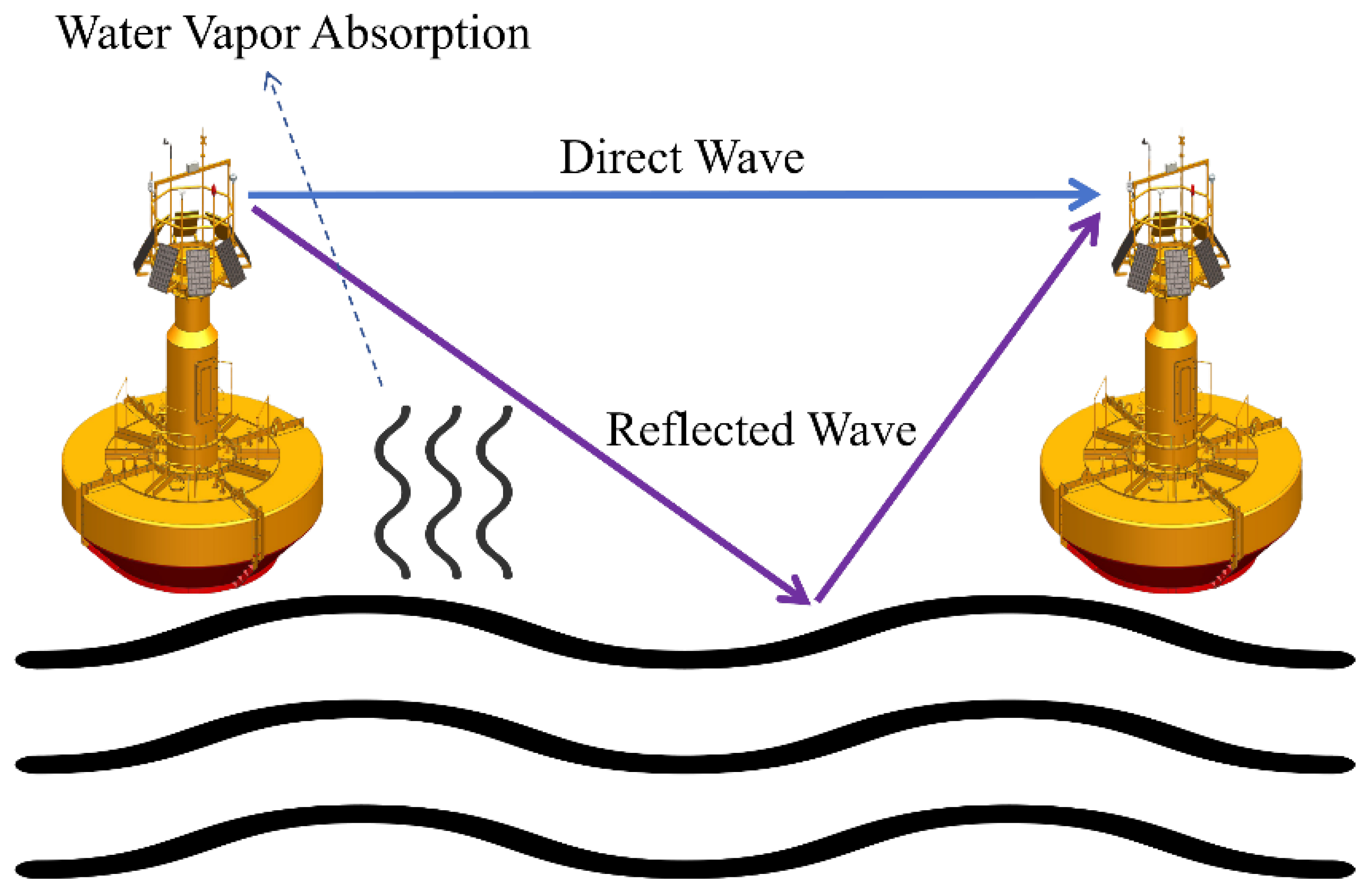
Under LoS conditions, the basic loss of the air-to-sea link is modeled by combining the Friis free-space propagation model with two-ray reflection and atmospheric water vapor absorption [31,33,34]. Accordingly, the LoS path loss can be expressed as:

$$L_{LoS}=L_{Friis}+\Delta L_{2ray}+L_{vap},$$

(5)

where $\Delta L_{2ray}$ denotes the additional loss correction caused by sea-surface two-ray reflection, and $L_{vap}$ denotes the attenuation caused by atmospheric water vapor absorption.

Under NLoS conditions, in addition to the basic propagation loss, additional environmental attenuation should also be considered. Therefore, the NLoS path loss can be expressed as:

$$L_{NLoS}=L_{LoS}+\eta$$

(6)

where $\eta$ denotes the additional attenuation factor under NLoS propagation. Its value depends on the specific sea-surface environment, wave conditions, and scattering characteristics. According to [32], $\eta =21$ dB is adopted in this study.

For radio propagation over the sea surface, the propagation loss model is developed based on the original SPM and further incorporates two-ray reflection and water vapor absorption [33,34,35]. Figure 2 illustrates the corresponding loss mechanism.

The mathematical expression of the SPM is given by:

$$L_s=A_1+A_2\lg d+A_3\lg H_b+A_4\mathrm{diffraction}+A_5\lg d\lg H_b+A_6{H}_m+A_7\mathrm{clutter},$$

(7)

where $L_s$ denotes the propagation loss, d is the distance between the transmitter and receiver, $H_b$ is the transmitter antenna height, and $H_m$ is the receiver antenna height. The terms diffraction and clutter represent the diffraction correction and environmental clutter correction, respectively [35], and are both set to 0 in this study. The parameters $A_1$ to $A_7$ are empirical model coefficients whose values depend on the specific propagation environment, as listed in

Table 2. SPM model parameters.

Parameter	Description	Value
$A_1$	Offset constant	33.9 lg f − 88.4
$A_2$	Multiplication factor	44.9
$A_3$	Transmitter antenna height factor	5.83
$A_4$	Multiplication factor for diffraction calculation	0
$A_5$	Multiplication factor	−6.55
$A_6$	Receiver antenna height factor	0
$A_7$	Multiplication factor for average terrain loss	1

.

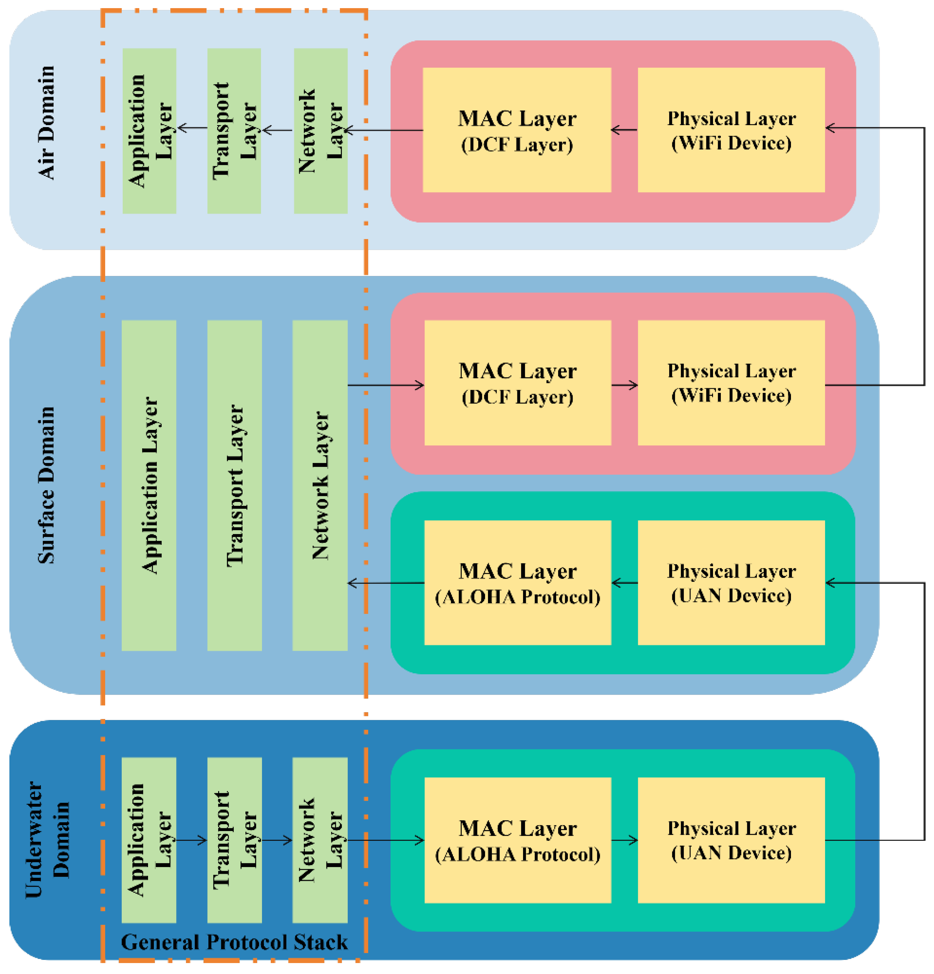
In NS-3, the underwater acoustic communication module UAN and the radio communication module WiFi have already been provided. However, to realize the functionality of an acoustic–radio collaborative transmission network, the key lies in enabling surface buoys to forward information received through underwater acoustic transmission via radio links. Therefore, surface buoy nodes must be equipped with both radio and underwater acoustic devices, so that they can serve as bridges between underwater and surface nodes. For buoy nodes, because radio communication and underwater acoustic communication differ in physical properties and transmission mechanisms, the two devices mounted on an acoustic–radio buoy operate with different MAC-layer protocols. The simulation framework of the acoustic–radio collaborative network is illustrated in Figure 3.

Aerial nodes belong to the radio transmission network, whereas underwater vehicles and underwater mobile nodes belong to the underwater acoustic transmission network. Buoy nodes simultaneously belong to both the radio transmission network and the underwater acoustic transmission network. At the physical layer, underwater acoustic nodes are equipped only with the UAN module, surface buoy nodes are equipped with both the underwater acoustic UAN module and the radio WiFi module, and aerial nodes are equipped with the WiFi module.

In the acoustic–radio collaborative network, the MAC protocol used for underwater acoustic communication is Aloha [36], whereas the surface radio network adopts the DCF mode of IEEE 802.11 [37]. The network layer is independent of the other layers and does not involve inter-layer dependency, thereby enabling the integration and interaction of underwater acoustic information and radio information within the acoustic–radio collaborative network. Surface buoy nodes are assigned two IP addresses, corresponding to the underwater acoustic device and the radio device, respectively. At the transport layer, the User Datagram Protocol (UDP) is employed to provide connectionless transmission services, while packet transmission and reception at the application layer are implemented through network sockets.

4. Q-Learning AODV Routing Protocol Design for Marine Acoustic–Radio Collaborative Networks

4.1. Principles of the Q-Learning Algorithm

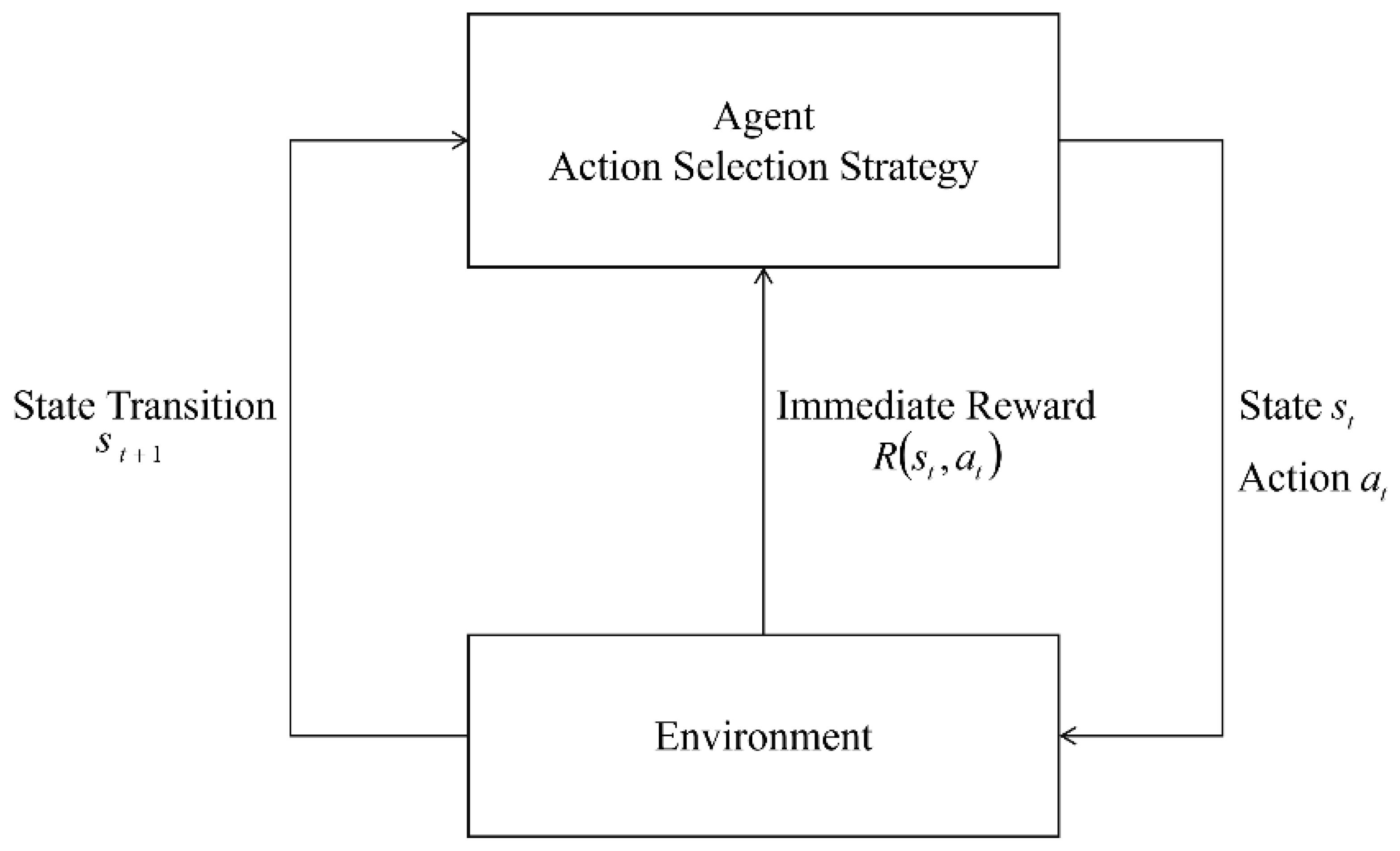
Q-Learning [38] is a model-free reinforcement-learning method that estimates a state-action value function from interaction data. For a transition from state $s_t$ to $s_{t+1}$ after action $a_t$ with immediate reward $r_t$, the tabular update is

$$Q_{t+1}(s_t,a_t)=(1-\alpha )Q_t(s_t,a_t)+\alpha \left[r_t+\gamma \underset{a\in \mathcal{A}\left(s_{t+1}\right)}{max}{Q}_t(s_{t+1},a)\right],$$

(8)

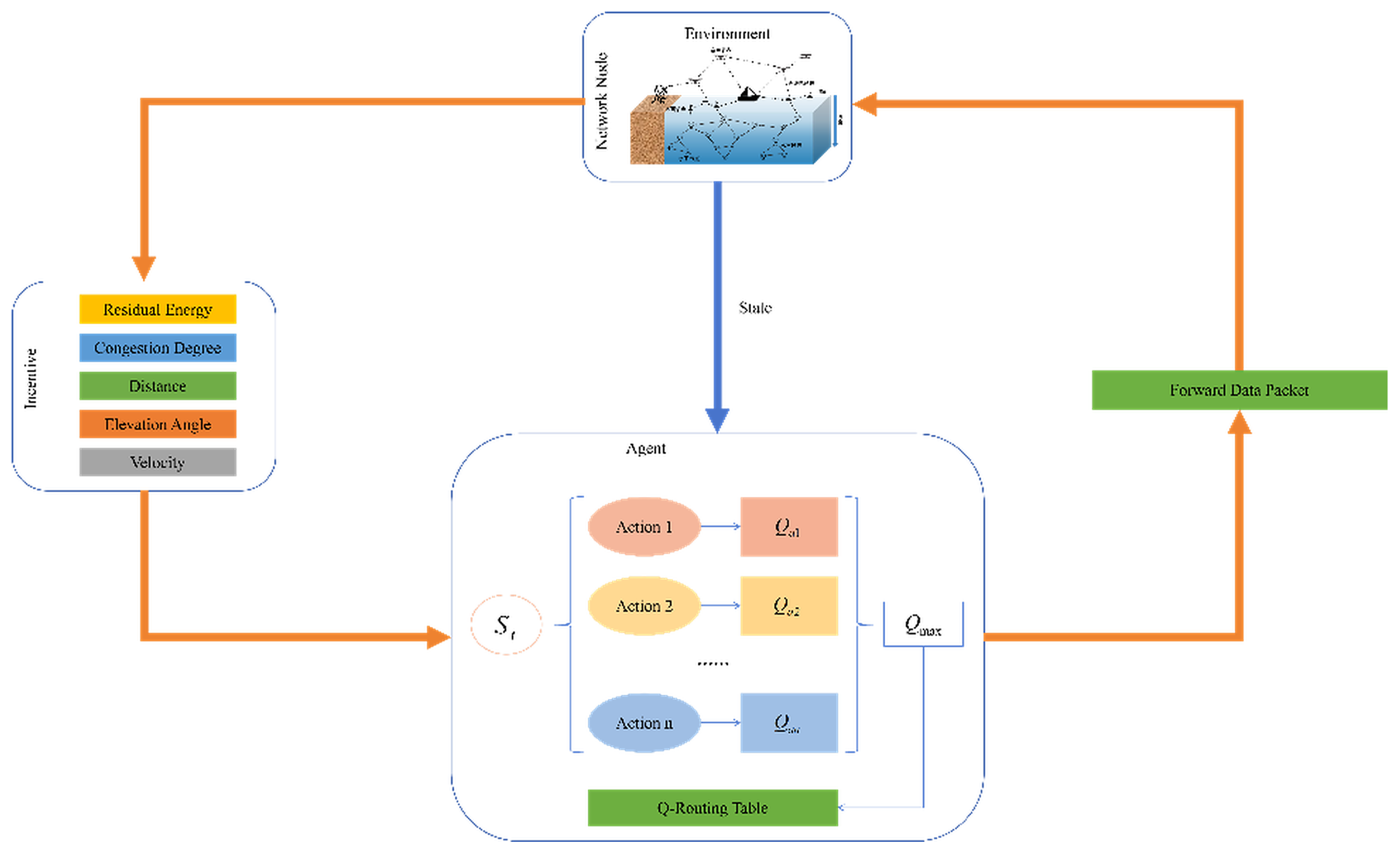
where $\alpha$ is the learning rate and $\gamma$ is the discount factor. In the routing problem considered here, the forwarding node acts as the agent, candidate next hops constitute the action set, and the immediate reward is computed from locally measured or received routing-state information. The online Q-value update is used to rank the currently available next-hop and route candidates as network conditions vary; we do not claim convergence to a stationary global optimum. Figure 4 shows the corresponding interaction process.

Standard tabular Q-Learning convergence results require assumptions such as sufficient state-action visitation and a stationary Markov environment [38]. Mobile marine networks with periodic HELLO messages, finite observations, changing queues, and time-varying links depart from these idealized assumptions. Therefore, convergence-related claims in this study are restricted to empirical adaptation under the evaluated conditions. The later-stage stabilization observed in the end-to-end performance curves is treated as an operational indication that the online value updates reach a relatively stable routing regime during the simulated interval; it is not interpreted as a proof of stationary-policy convergence.

4.2. Design of the Q-Learning AODV Routing Protocol

4.2.1. MDP, Local Observations, and Overall Framework

The routing decision is formulated as a locally observable MDP. At node x, a candidate-neighbor observation for forwarding through neighbor z is represented as

$$s_t^{(x,z)}=\left[{\sigma }_z,P_z,{\widehat{d}}_{xz},C_v(x,z),C_{\theta }(x,z),m_{xz}\right],$$

(9)

where ${\sigma }_z$ is the normalized residual-energy ratio and $P_z$ is the residual queue/buffer ratio (a larger value indicates more available buffer space). The normalized inter-node distance is ${\widehat{d}}_{xz}=d_{xz}/R_{xz}$, where $d_{xz}$ is the current distance between nodes x and z and $R_{xz}$ is the configured communication range of the corresponding link type. In addition, $C_v$ is the relative-velocity metric, $C_{\theta }$ is the elevation metric used for air–sea links, and $m_{xz}$ denotes the link type. The action $a_t=z$ selects one reachable one-hop neighbor as the next hop. The transition from $s_t$ to $s_{t+1}$ is induced by packet forwarding, energy consumption, queue evolution, node mobility, and route-control exchanges. The immediate reward is defined below, and the forwarding decision selects the candidate route or next hop with the largest currently stored Q-value.

The formulation is locally observable: a node does not require instantaneous global network state. Its own residual energy and queue occupancy are obtained locally; position and velocity are provided by the mobility/navigation subsystem in the simulation; neighbor values are disseminated through the extended RREQ, RREP, and HELLO messages; and inter-node distance is derived from the exchanged positions. In a practical deployment, fixed or pre-surveyed underwater/buoy positions can be used when available, while mobile underwater nodes require an acoustic/localization subsystem and aerial nodes can use GNSS/GPS. The corresponding navigation energy belongs to the platform-level energy budget and is treated separately from the communication-only lifetime metric used for routing comparison. This separation between learning logic and the physical entity that provides each observation follows the feasibility principle emphasized in [28]. The origin and dissemination of the routing-state variables are summarized in

Table 3. Origin and dissemination of routing-state variables.

Variable	Local Measurement/Estimate	Dissemination	Practical Note
Residual energy $\sigma$	Node energy model/energy monitor	RREQ, RREP, HELLO	Requires an energy estimator on the device
Queue availability P	Local routing/MAC buffer occupancy	RREQ, RREP, HELLO	Directly available from the local queue
Position	Mobility/navigation state in NS-3	RREQ, RREP, HELLO	Underwater mobility requires localization; aerial nodes may use GNSS/GPS
Velocity	Mobility/navigation state	RREQ, RREP, HELLO	Estimated locally from navigation/motion state
Distance d	Computed from local and neighbor positions	Not sent separately	Accuracy depends on localization accuracy
Q-value	Local Q-table	RREQ/RREP and HELLO route entries	Updated from received reward/downstream Q information

.

The selected state set is intentionally routing-oriented and emphasizes variables that can be measured locally or exchanged with bounded control overhead. Physical-channel effects such as packet error rate, instantaneous noise, Doppler spread, and acoustic propagation delay are not advertised as independent fields in every routing control packet. Where such effects are represented by the configured PHY/channel model, they influence packet reception and route outcomes indirectly, while distance, link type, queue state, and mobility provide the explicit routing observations. This separation keeps the state exchange lightweight and leaves room for richer channel-quality observations in deployments that can support the additional sensing and signaling cost.

The overall framework is shown in Figure 5.

In existing studies, residual node energy has been widely incorporated into routing evaluation metrics [18,19,20,21,24,25,26]. All nodes in the network are initially assumed to be fully charged, and energy is consumed thereafter during both standby operation and packet transmission/reception. The residual energy ratio is calculated as:

$${\sigma }_i={\displaystyle \frac{E_{\mathrm{current}}}{E_{\mathrm{initial}}}},$$

(10)

where $E_{\mathrm{current}}$ denotes the current residual energy of the node, $E_{\mathrm{initial}}$ denotes its initial energy, and ${\sigma }_i$ is the residual-energy ratio of node i.

The congestion state of a path is directly affected by the message load of nodes, and the congestion level is usually evaluated by the occupancy ratio of the packet buffer queue. Specifically, the queue length is defined as the number of packets waiting for transmission at a node. When a node cannot determine a valid route to the destination, packets are temporarily stored in the buffer. Once the buffer reaches its maximum capacity, i.e., the maximum queue length, buffer overflow occurs, causing subsequently arriving packets to be dropped and thereby affecting transmission efficiency and reliability. The buffer occupancy ratio is used to describe the proportion of occupied buffer space, which is calculated as:

$$P_i={\displaystyle \frac{L_{\mathrm{init}}-L_{\mathrm{curr}}}{L_{\mathrm{init}}}},$$

(11)

where $L_{\mathrm{curr}}$ denotes the current number of packets waiting in the queue, $L_{\mathrm{init}}$ denotes the configured maximum queue length, and $P_i$ is the residual buffer ratio of node i.

In terms of node mobility, a larger velocity difference between two nodes leads to a higher probability of link disconnection. Therefore, the velocity difference between two nodes is considered in the reward design. The reward function related to node mobility is defined as follows, where $V_A$ and $V_B$ denote the velocities of the two nodes, respectively:

$$\begin{array}{ccc}& C_v=\left\{\begin{array}{cc}1,& 0\le \mid V_A-V_B\mid <1\\ 1/\mid V_A-V_B\mid ,& \mid V_A-V_B\mid \ge 1\end{array}\right.& \end{array}$$

(12)

The elevation-angle term is applicable only to air–sea or sea–air radio links. For such a link, with ${\theta }_{AS}\in [0,\pi /2]$, the normalized metric is

$$C_{\theta }={\displaystyle \frac{{\theta }_{AS}}{\pi /2}}.$$

(13)

For underwater-to-underwater and air-to-air links, elevation is not used as a physical reward criterion. A link-type indicator ${\chi }_{\theta }(x,z)$ is therefore introduced, with ${\chi }_{\theta }=1$ for air–sea/sea–air links and ${\chi }_{\theta }=0$ for same-medium links. The reward aggregation below normalizes over the active components, so excluding the elevation term does not change the overall reward scale of same-medium links.

Finally, when the current node x receives a routing control message from its neighboring node z, node x extracts the information carried in the message and computes the incentive value, which is treated as the immediate reward $r_t$ in the Q-Learning algorithm. The Q-value of the route from node x to destination node y via node z is then updated according to

$$Q_x(y,z)=\alpha ·\{R(x,z)+{\gamma max}_{n\in N_z}{Q}_z(y,n)\}+(1-\alpha )·Q_x(y,z)$$

(14)

where $Q_x(y,z)$ denotes the Q-value at current node x for reaching destination node y via neighboring node z; z is a neighbor of node x; and $N_z$ denotes the set of neighbors of node z. Here, $\alpha$ is the learning rate and is set to 0.5 so that newly observed routing conditions and previously accumulated Q-values have equal update weight. The discount factor $\gamma$ is set to 1 because route evaluation is episodic over finite source-to-destination forwarding paths and the downstream route quality is not intentionally discounted. The distance threshold parameter $c=0.94$ activates the distance penalty only when a candidate link approaches the configured communication-range boundary. These parameters are treated as a fixed engineering baseline for the reported experiments; accordingly, the performance conclusions refer to this configuration rather than to a claim of global parameter optimality. The immediate reward fed back from node z to node x, denoted by $R(x,z)$, is calculated as

$$R(x,z)={\displaystyle \frac{w_{RQ}RQ+w_E{\sigma }_i+w_Q{P}_i+w_v{C}_v+{\chi }_{\theta }(x,z)w_{\theta }{C}_{\theta }}{H_k{W}_{\mathrm{act}}(x,z)}},$$

(15)

where

$$W_{\mathrm{act}}(x,z)=w_{RQ}+w_E+w_Q+w_v+{\chi }_{\theta }(x,z)w_{\theta }.$$

where $RQ$ is the link stability factor, which is defined as

$$RQ=\left\{\begin{array}{cc}1& 0\le d<c\times R\\ 1-{\displaystyle \frac{d}{R}}& c\times R\le d\le R\\ 0& d>R\end{array}\right.$$

(16)

where d is the distance between two nodes, R denotes the maximum communication range, and $0<c<1$. The term $cR$ represents the optimal communication distance, and c is the corresponding distance parameter. In this study, c is set to 0.94 so that the distance penalty is activated only when a link approaches the configured communication-range boundary; this is a heuristic engineering threshold rather than a universal optimum. In addition, ${\sigma }_i$ denotes the residual energy metric of node i, $P_i$ denotes the congestion-related metric of node i, $C_{\theta }$ denotes the elevation-angle metric between two nodes, $C_v$ denotes the velocity-difference metric between two nodes, and $H_k$ denotes the hop count from the destination node to the relay node.

The reward is a scalarization of multiple routing objectives. Before aggregation, all component metrics are normalized to $[0,1]$, preventing different physical units from dominating the sum. The baseline uses $w_{RQ}=w_E=w_Q=w_{\theta }=w_v=0.2$ as an equal-priority engineering configuration. The active-weight normalization $W_{\mathrm{act}}$ keeps the reward scale comparable across link types: for cross-medium links all five terms are active, whereas for same-medium links the elevation term is excluded and the remaining weights are renormalized automatically. The hop-count denominator discourages unnecessarily long paths. The reported results therefore characterize the complete multi-factor reward under this fixed baseline; they are not used to assign causal performance gains to any single reward component.

It can be seen from (15) that a neighboring node with higher residual energy, lower congestion level, shorter inter-node distance, larger elevation angle, and smaller velocity difference yields a larger reward $R(x,z)$. Accordingly, a larger Q-value indicates a better route to the destination node. Each node periodically updates the Q-values in its routing table. When a source node needs to transmit data, it selects the path with the highest Q-value in the current routing table as the forwarding path.

4.2.2. Protocol Workflow Design

The overall procedure of the Q-Learning AODV protocol mainly consists of two processes. The first is the route discovery process, which is triggered when the routing table of a node does not contain route information to the destination. This process is used to search for routes, record the paths to the destination, and maintain multiple node-disjoint paths toward the destination. The second is the route updating process, which is mainly accomplished through HELLO packet exchanges and is used to dynamically update neighbor information and the Q-values of routing entries.

Since the proposed method needs to select the route with the highest Q-value from multiple reachable paths, the original AODV protocol is extended to support the storage of multiple node-disjoint paths.

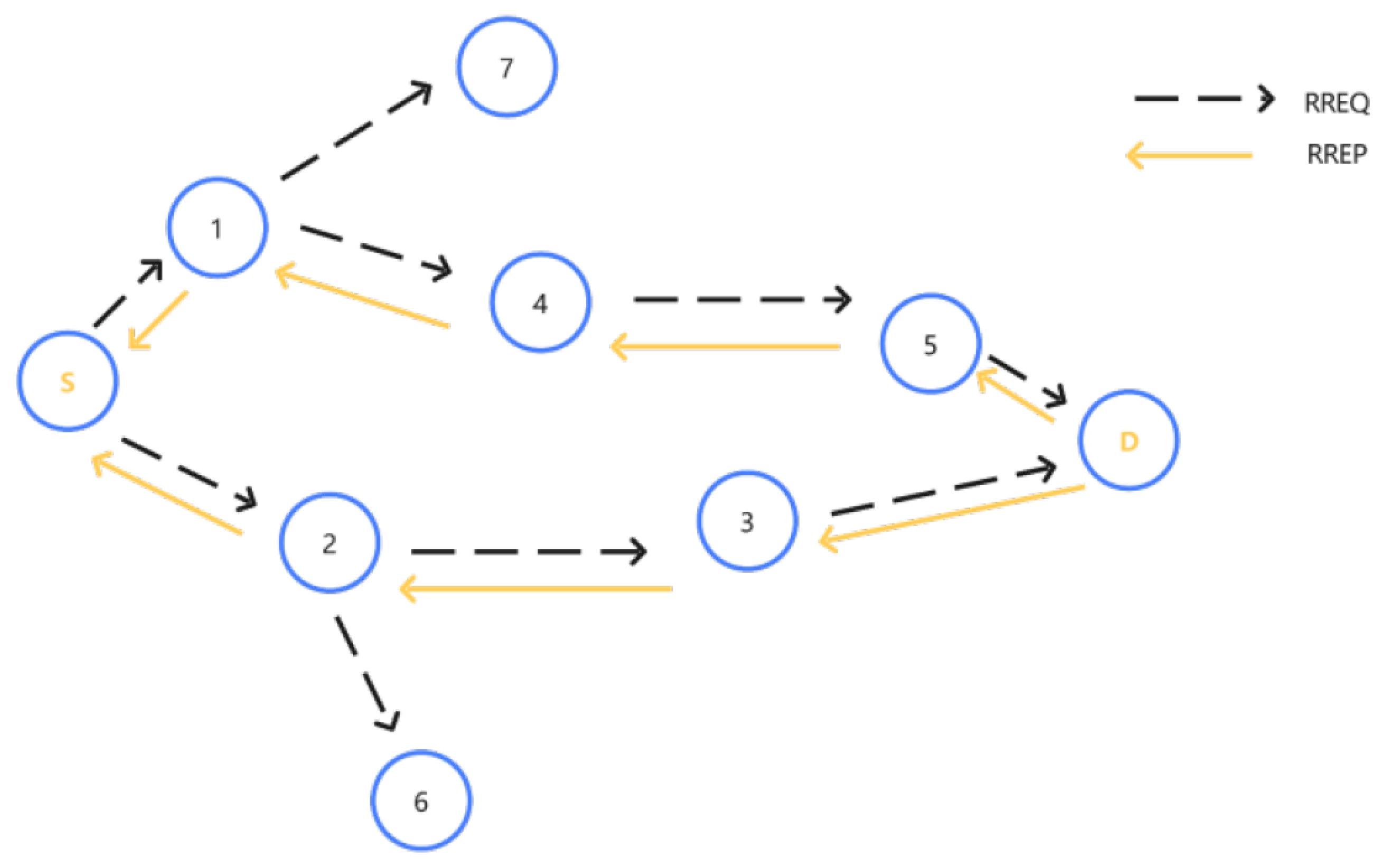
The operating mechanism of the multipath protocol can be divided into two core modules, namely route establishment and route maintenance. During the route establishment phase, the source node broadcasts Route Request (RREQ) packets. After receiving an RREQ packet, an intermediate node first performs duplicate detection. If the packet has already been processed, it is discarded immediately; otherwise, the reverse routing entry is created or refreshed. If the node is neither the destination nor has a valid route cache to the destination, it updates the header information of the RREQ packet and continues forwarding it. Otherwise, it generates a Route Reply (RREP) packet and sends it back to the source. When an intermediate node receives an RREP packet, it updates the forward routing table entry accordingly and determines whether it is the source node. If it is not the source node, it updates the protocol fields of the RREP packet and continues forwarding it. Once the source node receives the RREP packet, the multipath topology is established, as illustrated in Figure 6.

Compared with the original AODV protocol, the proposed scheme adopts a mechanism in which intermediate nodes process only the first received RREQ and ignore subsequent duplicate RREQs, while the destination node is allowed to process multiple RREQ packets with the same source node and identifier. In this way, multiple loop-free and node-disjoint transmission paths can be generated. As shown in Figure 6, two such optimized paths are established between source node S and destination node D. This selective processing strategy not only ensures path quality but also improves network resource utilization.

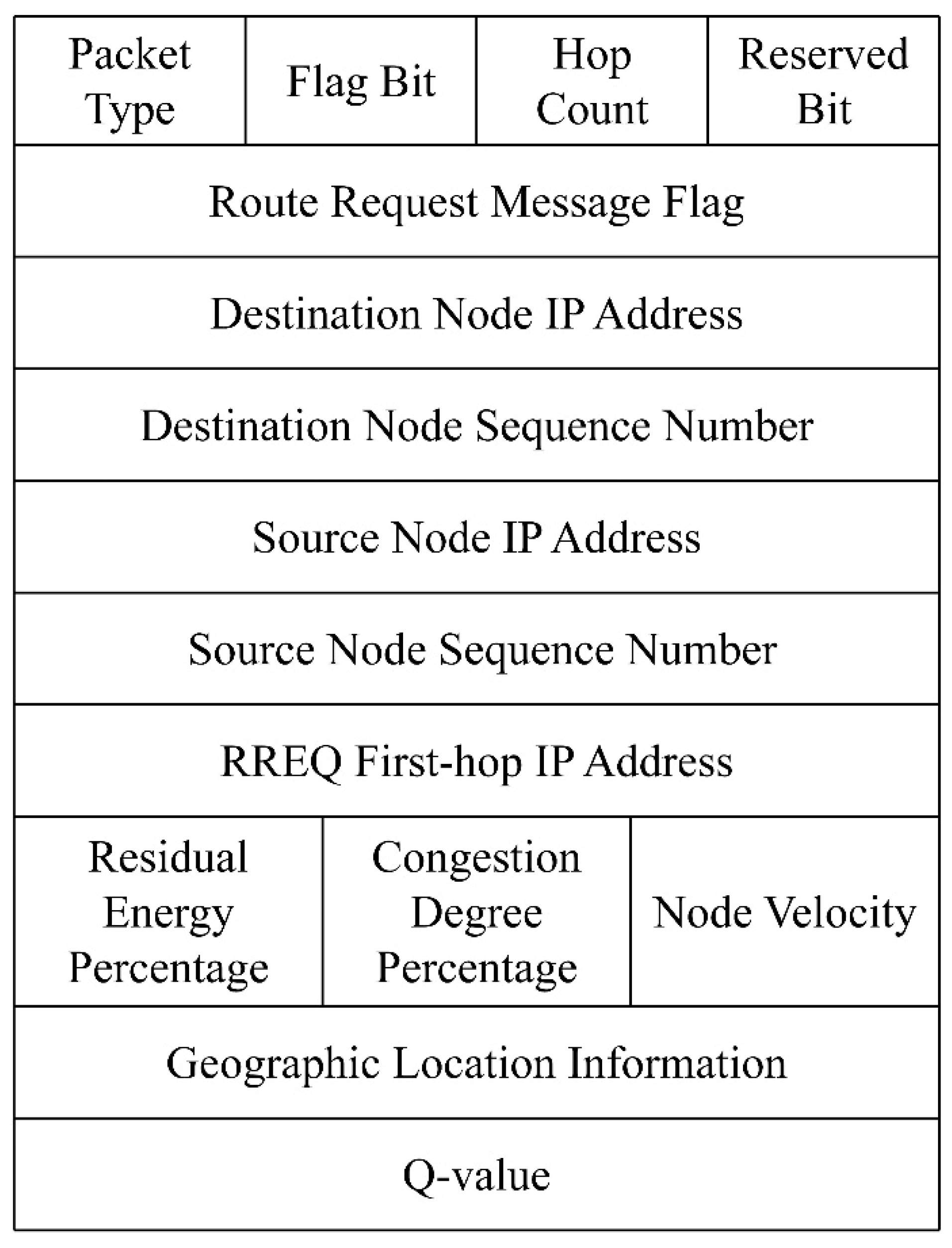
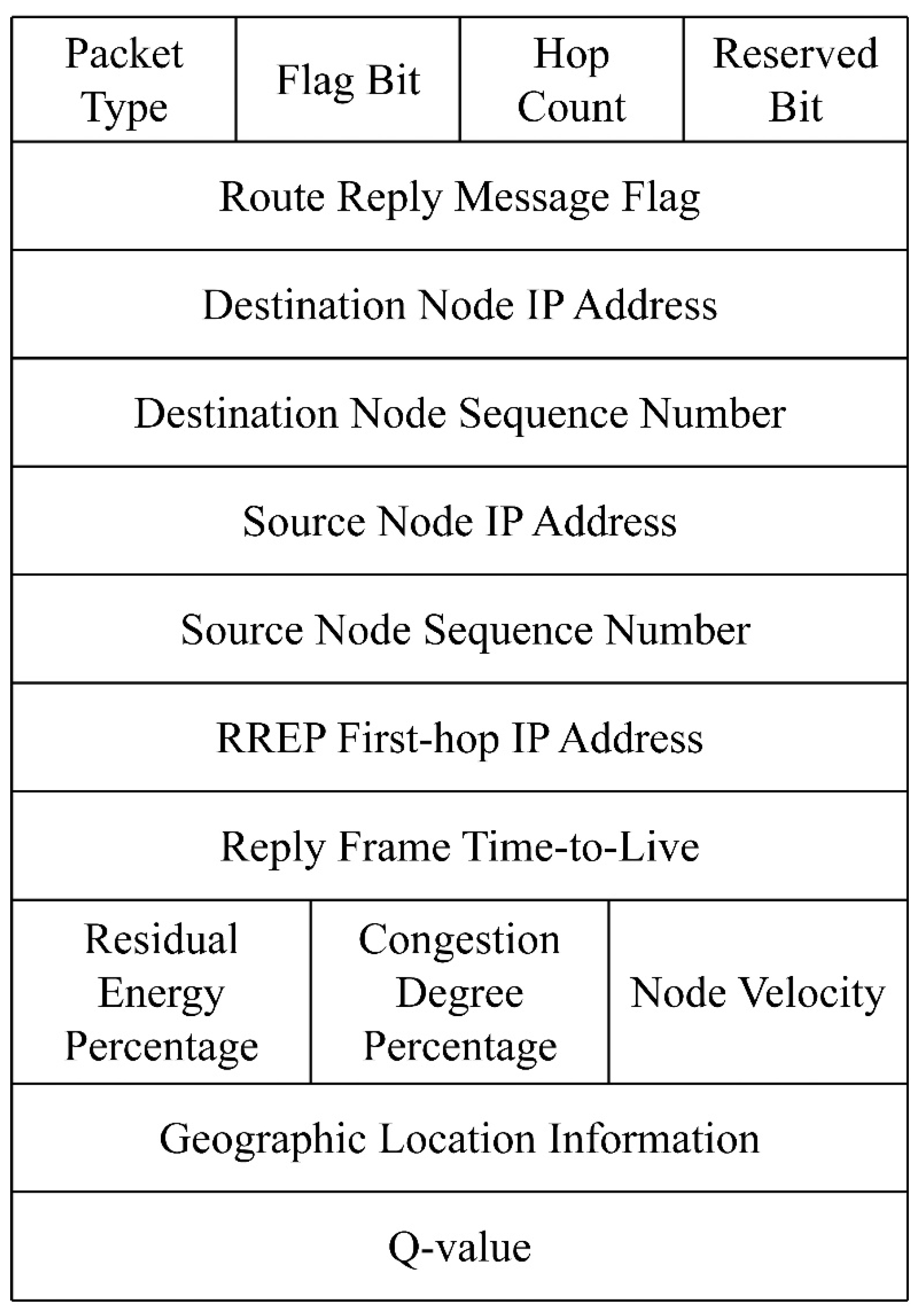
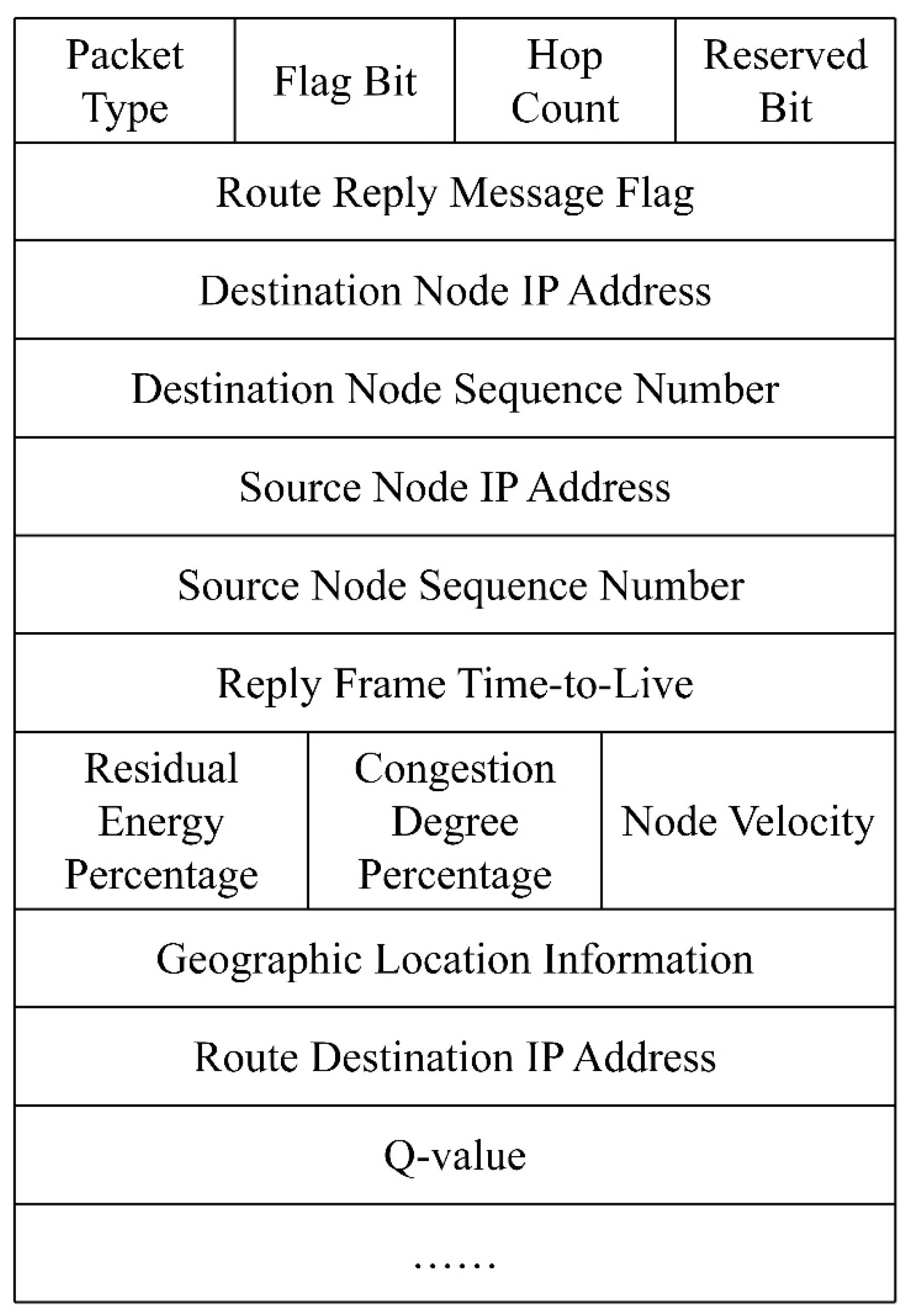
In the Route Request (RREQ) and Route Reply (RREP) packets, fields for residual energy, node congestion level, geographic location, node velocity, first-hop IP address, and Q-value are added. In the HELLO packet, fields for residual energy, node congestion level, geographic location, node velocity, as well as destination addresses in the routing table and their corresponding Q-values are included. The modified packet formats are shown in Figure 7, Figure 8 and Figure 9.

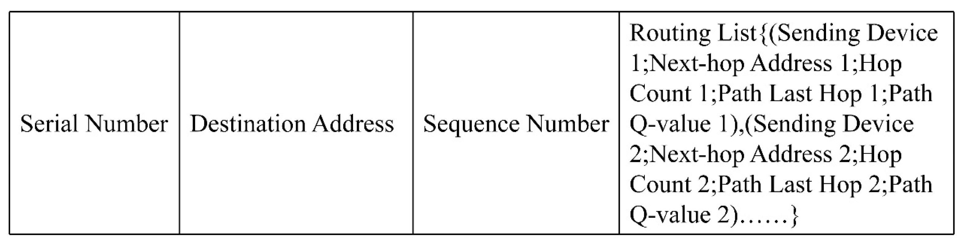
A multipath routing table usually contains detailed information for multiple paths. As shown in Figure 10, the routing table is redesigned so that each destination address corresponds to multiple candidate paths. Each path is associated with several parameters, including the sending interface, next-hop address, hop count, last hop of the path, and path Q-value. These parameters enable network devices to accurately select the path with the highest Q-value for data forwarding.

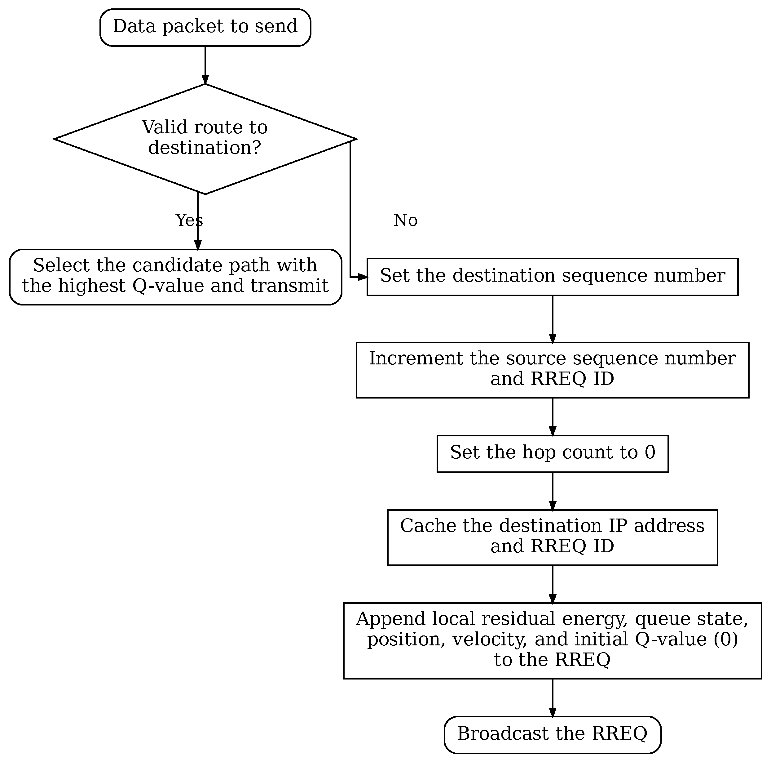
The route discovery process is triggered when a node needs to send a data packet but has no route information to the destination in its routing table. In this case, the source node broadcasts an RREQ packet to explore route information and appends its own residual energy, congestion level, location information, velocity, and initial Q-value to the RREQ packet, where the initial Q-value is set to 0. The source-node route-discovery procedure is illustrated in Figure 11.

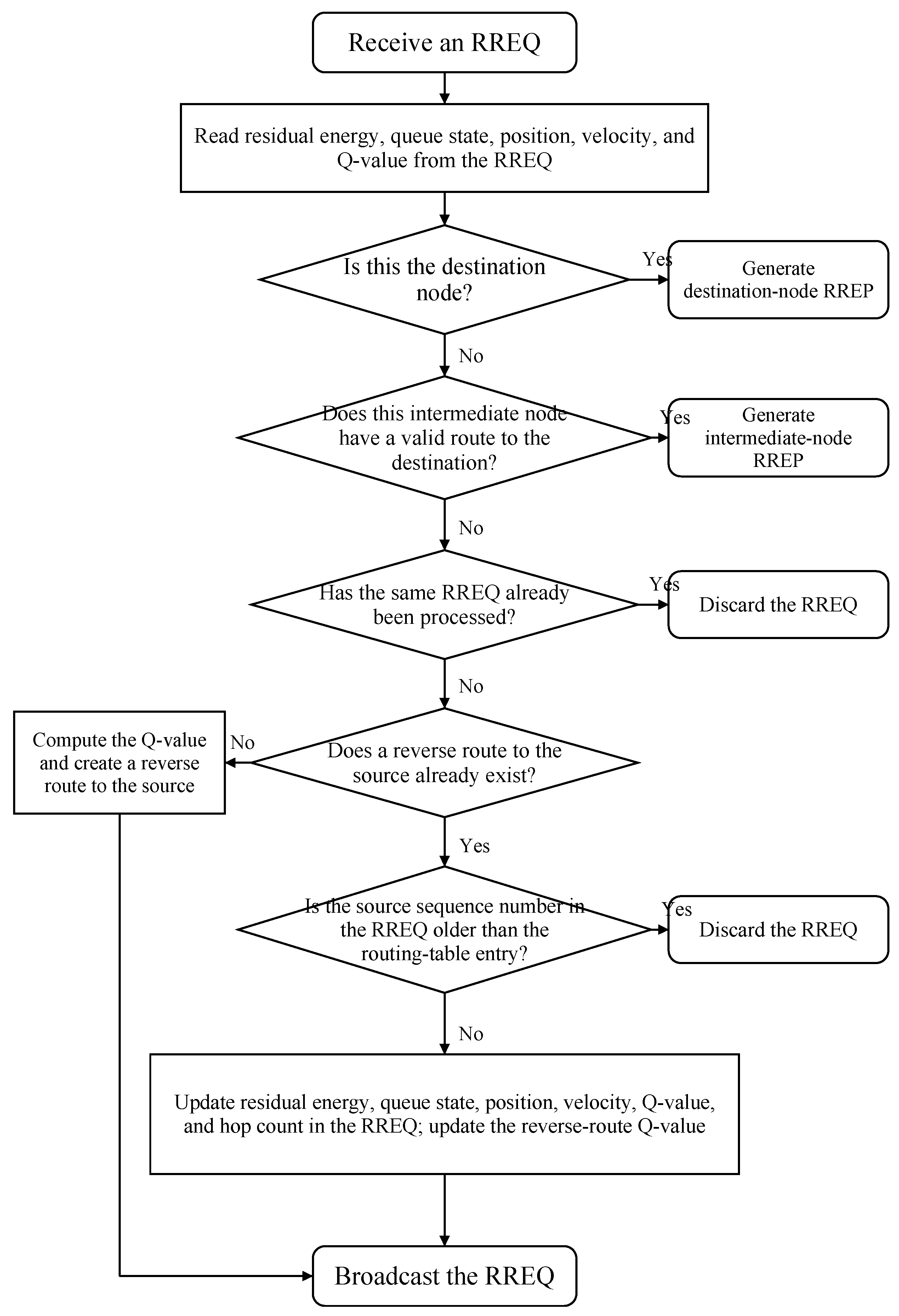
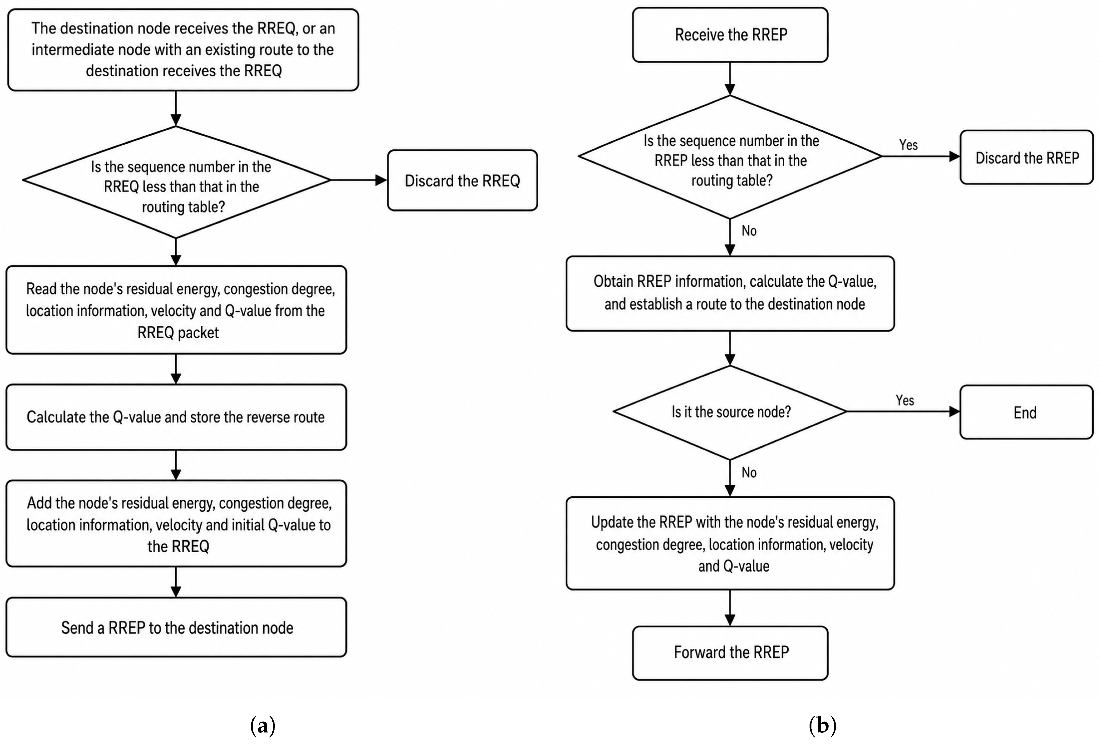
After receiving an RREQ packet, a neighboring node reads the residual energy, congestion level, location information, node velocity, and Q-value carried in the packet. It first determines whether it is the destination node of the RREQ, or whether its routing table already contains a route to the destination. If neither condition is satisfied, the node further checks whether it has previously received an RREQ with the same source node and identifier. If so, the packet is discarded. Otherwise, the node calculates the immediate reward, updates its Q-value toward the source node, establishes a reverse route, appends the updated Q-value together with its residual energy, congestion level, location information, and node velocity to the RREQ packet, and then continues broadcasting it. This process is repeated until the destination node is reached. The corresponding RREQ processing procedure at a receiving node is shown in Figure 12.

If the current node already has a route to the destination specified in the RREQ packet, it calculates the Q-value of the path to the source node and records the route to the source node in the routing table. It then inserts into the RREP packet the Q-value of its latest and highest-Q path to the destination, together with its residual energy, congestion level, location information, and node velocity, and sends the RREP packet as a reply. When the node itself is the destination, it continues processing subsequently received RREQ packets and includes its residual energy, congestion status, location information, and velocity in the RREP packet to complete the route reply. Meanwhile, the node updates its Q-value toward the source node, thereby establishing the reverse path. For each received RREQ packet, the destination node generates and sends a corresponding RREP packet in response.

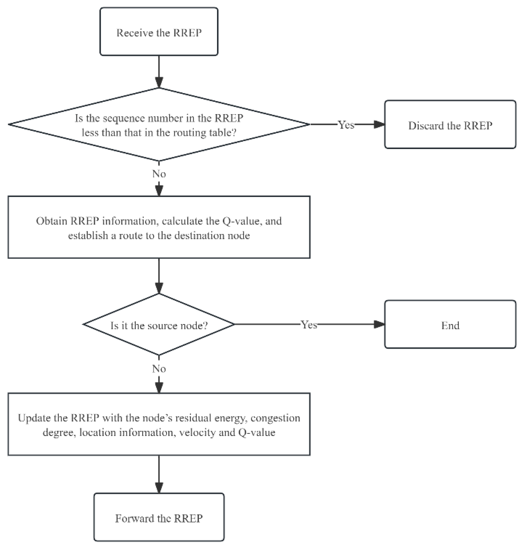
If a node receives an RREP packet returned by the destination node, it reads the residual energy, congestion level, location information, and node velocity carried in the RREP packet, calculates the immediate reward, and updates its Q-value toward the destination according to the Q-value update equation, thereby establishing the forward route. If the node is not the source node, it adds the updated Q-value together with its residual energy, congestion level, location information, and node velocity to the RREP packet and unicasts it onward until it reaches the source node. As these RREP packets arrive at the source node, each RREP establishes a corresponding forward route. Through this design, the source node can obtain multiple node-disjoint paths to the destination. The corresponding target-node RREQ and intermediate-node RREP processing flows are summarized in Figure 13.

The route updating process is illustrated in Figure 14 and is mainly accomplished through HELLO packet exchanges. All active nodes periodically broadcast HELLO packets, which carry information such as residual energy, node congestion level, location information, node velocity, and Q-values stored in the routing table. After receiving a HELLO packet, a node determines whether there exists a route in its routing table whose next hop is the neighboring node that sent the HELLO packet. If such a route exists, the node reads the residual energy, congestion level, location information, and node velocity contained in the HELLO packet, calculates the immediate reward, and updates its own Q-value table according to the Q-values of the corresponding routes carried in the HELLO packet and the Q-value update equation. Otherwise, no further processing is performed.

If a node does not receive a HELLO packet from a neighboring node within a certain period, the route maintenance procedure is triggered and the associated paths are removed; the specific process is similar to that of the AODV routing protocol. Through the HELLO-based updating mechanism, all paths in the routing table remain in a dynamically updated state, ensuring that the Q-values of all routes are adjusted in real time according to network conditions. This mechanism enables the protocol to sufficiently explore other potentially better paths and, to the greatest extent possible, avoid falling into a local optimum.

4.2.3. Signaling, Computational Complexity, and Reproducibility

The proposed protocol does not introduce a new control-packet type, but it does enlarge existing control packets. Let $b_E$, $b_Q$, $b_p$, $b_v$, $b_f$, and $b_{Qv}$ denote the serialized byte lengths of residual energy, congestion, position, velocity, first-hop address, and Q-value fields, respectively. The additional RREQ/RREP payload can therefore be written as

$$B_{\mathrm{add}}^{\mathrm{RREQ}/\mathrm{RREP}}=b_E+b_Q+b_p+b_v+b_f+b_{Qv}.$$

(17)

For HELLO messages, if M destination/Q-value pairs are included, the additional payload is

$$B_{\mathrm{add}}^{\mathrm{HELLO}}=b_E+b_Q+b_p+b_v+M(b_d+b_{Qv}),$$

(18)

where $b_d$ is the destination-address size. The numerical value of this overhead depends on the serialization widths selected for these fields, whereas Equations (17) and (18) make the protocol-level overhead contribution explicit independently of a particular data-type implementation. The control-overhead fraction is defined as ${\eta }_{ctrl}=B_{ctrl}/(B_{ctrl}+B_{data})$. Accordingly, the earlier statement “without extra signaling overhead” is replaced throughout by the more accurate statement “without introducing additional packet types.”

Let D be the number of known destinations, K the maximum number of maintained candidate paths per destination, and $\Delta$ the local neighbor degree. Standard AODV maintains approximately one active route entry per destination, giving $O\left(D\right)$ routing-state storage. Q-Learning AODV stores up to K path/Q entries per destination, giving $O\left(DK\right)$ storage. Selecting the best stored path is $O\left(K\right)$, and a Q update that searches the downstream neighbor action values is $O(\Delta )$ in a direct table implementation. Packet-header processing remains $O\left(1\right)$ per fixed field, while HELLO serialization can grow with the number of destination/Q-value pairs carried. The method therefore trades additional memory, control bytes, and local computation for adaptive multipath routing. Importantly, maintaining several candidate paths does not imply data-packet replication in the present protocol: one highest-Q path is selected for a packet flow at a given decision instant, so redundancy arises from route state and control information rather than deliberate payload duplication.

Pseudocode of Q-Learning AODV

• At node x, obtain local energy, queue occupancy, position, and velocity; update the corresponding fields in the outgoing AODV control message.
• On receiving an RREQ/RREP/HELLO from neighbor z, extract the advertised state, compute distance and link type, normalize active reward components, and calculate $R(x,z)$.
• Update $Q_x(y,z)$ using the tabular Q-Learning rule and the best downstream Q-value reported/known for destination y.
• During route discovery, preserve admissible node-disjoint candidate paths and their Q-values; during HELLO maintenance, refresh neighbor state and remove expired paths.
• For data forwarding, choose the valid path with the maximum current Q-value. If no valid path remains, trigger standard AODV route discovery.

5. Performance Evaluation of the Q-Learning AODV Routing Protocol

5.1. Simulation Environment and Performance Metrics

Simulation experiments of the Q-Learning AODV routing protocol are conducted on a marine cross-medium acoustic–radio collaborative network. During node deployment, in order to better reflect the performance of the acoustic–radio collaborative network and to ensure that packets traverse multiple underwater hops, a relatively large number of underwater nodes are deployed at different depths, where the shallower underwater nodes can serve as relay nodes.

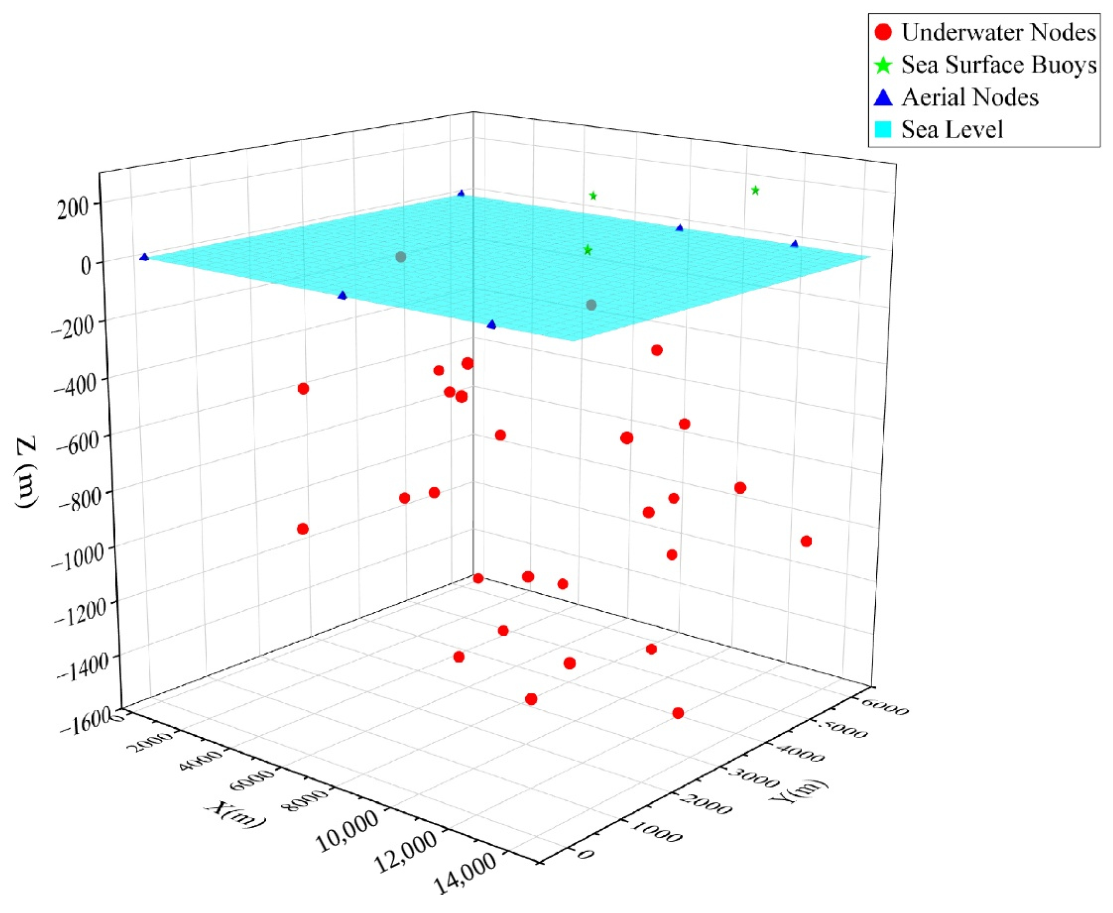
The overall topology of the simulation scenario is shown in Figure 15. The marine cross-medium acoustic–radio collaborative network consists of 28 underwater nodes, 6 surface buoy nodes, and 3 aerial nodes. The detailed simulation parameters are listed in

Table 4. Simulation parameters.

Parameter	Value
Underwater acoustic center frequency	25 kHz
Underwater acoustic bandwidth	5 kHz
Underwater acoustic MAC	Aloha
Radio MAC	802.11-DCF
Radio symbol rate	2 Mbps
Underwater acoustic data rate	10,000 bps
Underwater acoustic transmission range	2.2 km
Configured radio-link range	7.8 km
Initial energy of source and destination nodes	90,000 J
Initial energy of other relay nodes	900 J
Simulation duration	900 s
Packet sending interval	2.5 s
Packet size	40 bytes (320 bit)
Water depth of the source node	1000 m
Speed of underwater nodes and buoys	2–3 m/s
Speed of aerial nodes	50 m/s

.

The underwater PHY setting in Table 4 is used as a common NS-3 UAN transmission mode for routing-level protocol comparison. The 10 kb/s entry is therefore not intended as a modem-level spectral-efficiency claim for a particular 5-kHz BFSK transducer. A hardware-specific BFSK implementation would require the data rate to be selected jointly with the actual modulation, coding, transducer bandwidth, and receiver design. The results in this paper should accordingly be interpreted as relative routing performance under the stated common PHY configuration.

The acoustic channel abstraction is designed for routing-level comparison. The Thorp component captures distance- and frequency-dependent spreading/absorption, while node mobility makes the link geometry time varying during the run. Finer-scale effects such as multipath structure, Doppler spread, and ambient-noise variation are not parameterized as separate stochastic state processes in the routing model; consequently, the reported conclusions are confined to the stated NS-3 PHY/channel abstraction rather than extrapolated to a specific measured ocean channel. The configured 7.8 km radio-link range is likewise an idealized connectivity setting and should not be interpreted as a typical IEEE 802.11 coverage distance. A link of this length would require a favorable link budget, suitable high-gain or directional antennas, and long-distance MAC timing/ACK configuration. The value is retained only as a common topology parameter: all compared routing protocols use the same lower-layer radio setting, so it does not preferentially benefit one routing protocol, although it limits direct physical extrapolation. Table 4 summarizes the scenario-defining parameters used for this comparison.

Packet delivery ratio (PDR) and end-to-end delay are treated as the primary performance metrics in this study. Communication-subsystem lifetime is retained as a secondary protocol-efficiency metric because routing decisions directly change transmission, reception, idling, and route-maintenance activity. For a node over an observation interval, the communication-energy decrement is expressed as $\Delta E_i=P_{\mathrm{tx}}{T}_{\mathrm{tx}}+P_{\mathrm{rx}}{T}_{\mathrm{rx}}+P_{\mathrm{idle}}{T}_{\mathrm{idle}}$, and the first modeled communication node reaching energy depletion determines $T_{\mathrm{life}}$ in Equation (22). This metric does not include propulsion, vehicle-control, or GNSS/navigation power. Those platform-level loads can dominate the battery consumption of an aerial or mobile vehicle; therefore, the reported lifetime values quantify routing-related communication-energy balancing only and must not be interpreted as complete mission endurance. Accordingly, the communication-energy results are interpreted comparatively under the common energy-model configuration applied to all protocols, rather than as absolute hardware-level power measurements.

To evaluate the performance and advantages of the proposed Q-Learning AODV routing protocol, a comparative analysis is conducted against conventional routing protocols, including AODV, OLSR, and DSDV. The evaluation is based on the following key network performance metrics:

a. Average end-to-end delay

The average end-to-end delay is computed over the packets that are successfully received:

$$D_{\mathrm{avg}}={\displaystyle \frac{1}{n}}{\displaystyle \sum _{i=1}^n}\left(t_{r,i}-t_{s,i}\right),$$

(19)

where n is the number of successfully received packets, $t_{r,i}$ is the reception time of packet i, and $t_{s,i}$ is its transmission time.

b. Packet delivery ratio

The packet delivery ratio (PDR) is the percentage of source packets that are successfully received at the destination:

$$\mathrm{PDR}={\displaystyle \frac{P_r}{P_s}}\times 100\%,$$

(20)

where $P_r$ is the number of packets received at the destination and $P_s$ is the number of packets generated by the source.

c. Throughput

The average application-layer throughput is calculated as

$$T_{\mathrm{put}}={\displaystyle \frac{P_r{S}_d\times 8}{T}},$$

(21)

where $S_d$ is the packet size in bytes and T is the measurement interval in seconds.

d. Communication-subsystem lifetime

As a secondary protocol-efficiency metric, communication-subsystem lifetime is defined by the first modeled communication node whose residual communication-energy budget is depleted:

$$T_{\mathrm{life}}=min\left\{t|\exists i,E_i\left(t\right)\le 0\right\}.$$

(22)

Here, $E_i\left(t\right)$ is the residual communication-energy budget of node i at time t. The metric excludes propulsion and navigation loads and therefore measures only the lifetime of the modeled communication subsystem.

To comprehensively evaluate the performance of the proposed Q-Learning AODV protocol in cross-medium acoustic–radio collaborative networks, this study designs three systematic simulation experiments. All experiments are conducted on an NS-3-based cross-medium comparative simulation framework that combines the UAN and WiFi modules with the stated acoustic/radio propagation and communication-energy abstractions.

Experiment 1: Performance comparison with conventional routing protocols

This experiment is designed to verify the comprehensive performance advantages of Q-Learning AODV over conventional routing protocols in cross-medium networks. AODV, OLSR, and DSDV are selected as representative baseline protocols, and the comparison is carried out under a unified network topology (as shown in Figure 15) and identical traffic load conditions. To cover typical link patterns in cross-medium communication, three communication scenarios are considered in this experiment, namely underwater-to-underwater, underwater-to-air, and air-to-underwater communications. All protocols are evaluated under the same node deployment density, traffic flow pattern, and environmental dynamics configuration, so as to objectively reflect the performance differences of the protocols themselves. The performance metrics include packet delivery ratio, average end-to-end delay, network throughput, and communication-subsystem lifetime.

Experiment 2: Combined network-size and coverage stress test

Four increasingly demanding configurations are designed as listed in

Table 5. Network scale configurations.

Group	Surface Buoys	Aerial Nodes	Underwater Nodes	Network Coverage Area $(\mathit{L}\times \mathit{W}\times \mathit{D})$
1	2	1	8	$6\mathrm{km}\times 2\mathrm{km}\times 1.5\mathrm{km}$
2	4	2	16	$6\mathrm{km}\times 6\mathrm{km}\times 1.5\mathrm{km}$
3	6	3	28	$12\mathrm{km}\times 6\mathrm{km}\times 1.5\mathrm{km}$
4	8	4	40	$18\mathrm{km}\times 6\mathrm{km}\times 1.5\mathrm{km}$

. Both node count and coverage area change across groups. Therefore, this experiment is a combined size-and-coverage stress test rather than a controlled isolation of a single “network-scale” variable: node density, expected hop count, and contention can change simultaneously. For representativeness and comparison consistency, Experiment 2 focuses on the underwater-to-underwater communication scenario, so as to investigate the behavior of Q-Learning AODV under increasingly demanding joint node-count and coverage-area configurations.

Experiment 3: Validation of dynamic topology adaptability

To investigate the performance of the protocol in highly dynamic marine environments, this experiment focuses on the impact of node mobility on routing performance. The speed of underwater nodes varies from 2 m/s to 6 m/s, while the other network and environmental parameters remain the same as those in Experiment 1. To highlight the topology variation characteristics of dynamic underwater acoustic networks and facilitate comparative analysis, Experiment 3 also adopts the underwater-to-underwater communication scenario. By comparing the performance of different routing protocols under different node mobility conditions, the robustness and adaptability of the proposed Q-Learning AODV protocol in highly dynamic marine topologies are evaluated.

The above three experiments evaluate the proposed Q-Learning AODV protocol from three complementary perspectives: cross-protocol performance under representative cross-medium scenarios, response to joint size/coverage stress, and adaptability to increasing node mobility.

5.2. Simulation Results and Analysis

5.2.1. Performance Comparison Between Q-Learning AODV and Conventional Routing Protocols

Packet Delivery Ratio Analysis

Table 6. Packet delivery ratio.

Scenario	Q-Learning AODV	AODV	OLSR	DSDV
Underwater-to-underwater	88.3%	55.8%	24.1%	18%
Underwater-to-air	76.1%	68.3%	61.9%	16.9%
Air-to-underwater	91.9%	86.9%	50.8%	0

presents the packet delivery ratio of Q-Learning AODV and three conventional routing protocols, namely AODV, OLSR, and DSDV, under three scenarios: underwater-to-underwater, underwater-to-air, and air-to-underwater communications. In all three scenarios, the proposed Q-Learning AODV protocol achieves a higher packet delivery ratio than the other three routing protocols.

In the underwater-to-underwater scenario, the packet delivery ratio of Q-Learning AODV reaches 88.3%, which is 32.5 percentage points higher than AODV and corresponds to a 58.2% relative improvement. In the underwater-to-air scenario, the PDR is 76.1%, 7.8 percentage points (11.4% relatively) above AODV. In the air-to-underwater scenario, Q-Learning AODV reaches 91.9%, 5.0 percentage points (5.8% relatively) above AODV.

For DSDV, the packet delivery ratio drops to 0 in the air-to-underwater scenario. This is because both OLSR and DSDV are table-driven routing protocols that require continuous maintenance of global routing tables, resulting in considerable routing overhead and making packet collisions more likely in underwater acoustic channels. Overall, Q-Learning AODV outperforms the conventional AODV protocol in all three scenarios, demonstrating superior performance. This is mainly because the proposed protocol considers multiple reward factors and selects the path with the highest Q-value for data transmission. As a result, its routes are more stable than those of the other conventional routing protocols, leading to a consistently higher packet delivery ratio.

Throughput

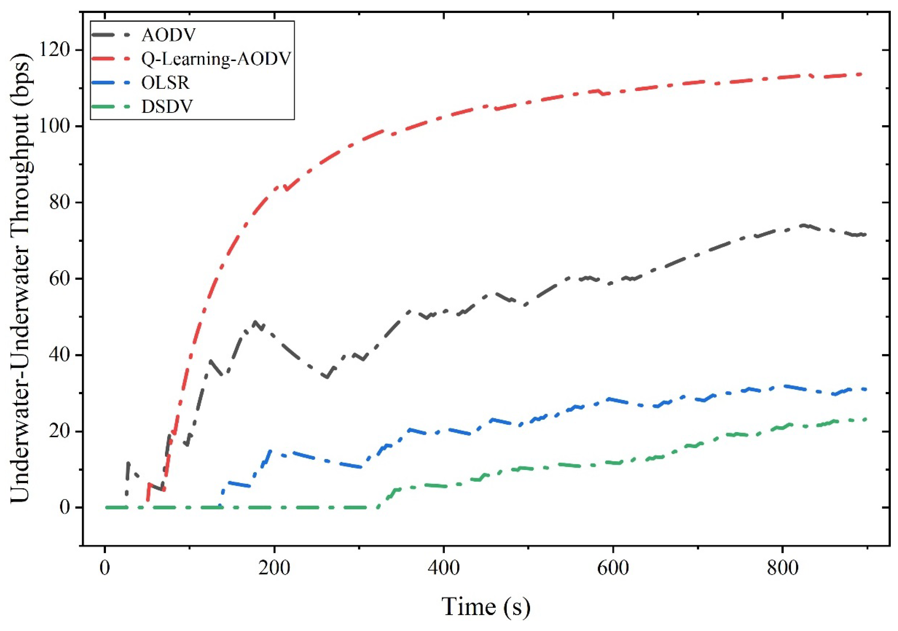
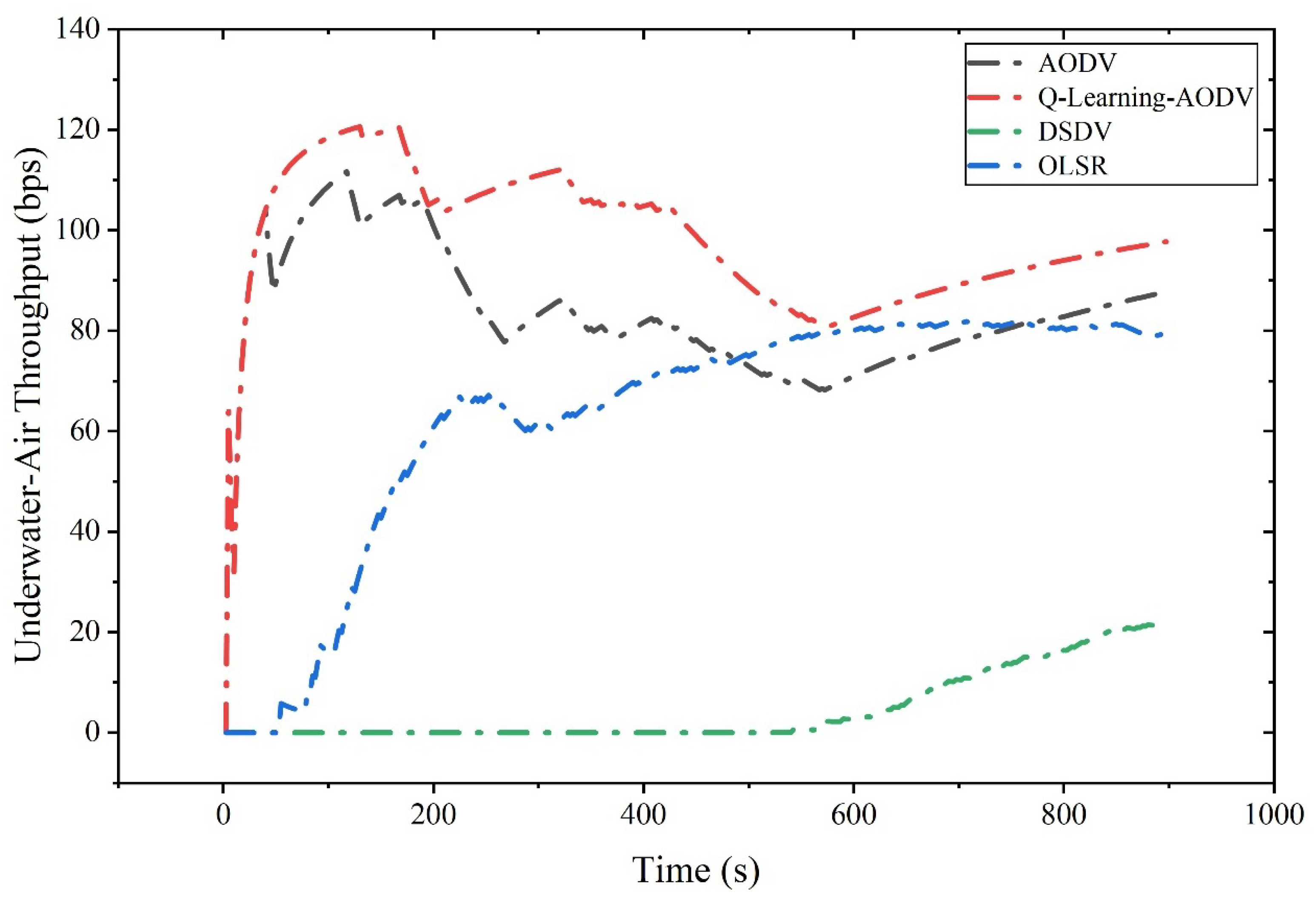
The throughput comparison for the underwater-to-underwater transmission scenario is shown in Figure 16. As time progresses, the throughput of Q-Learning AODV gradually increases and begins to outperform that of the conventional AODV protocol after approximately 100 s, before eventually stabilizing in the later stage. The throughput of the conventional AODV protocol also increases steadily in the later stage, but its overall performance remains inferior to that of Q-Learning AODV. In contrast, the traditional OLSR and DSDV protocols perform consistently worse than Q-Learning AODV throughout the simulation. Overall, Q-Learning AODV exhibits more stable and efficient throughput during long-term operation.

The throughput comparison for the underwater-to-air transmission scenario is shown in Figure 17, which presents the throughput performance of the four protocols over time. At the initial stage, the throughput difference between AODV and Q-Learning AODV is relatively small. As time progresses, however, the throughput of Q-Learning AODV becomes higher than that of AODV. The throughput of OLSR also exhibits an increasing trend before gradually stabilizing, but its overall performance still remains inferior to that of Q-Learning AODV. By contrast, DSDV stays at a relatively low level throughout the entire process. The throughput of all four routing protocols tends to stabilize after approximately 600 s.

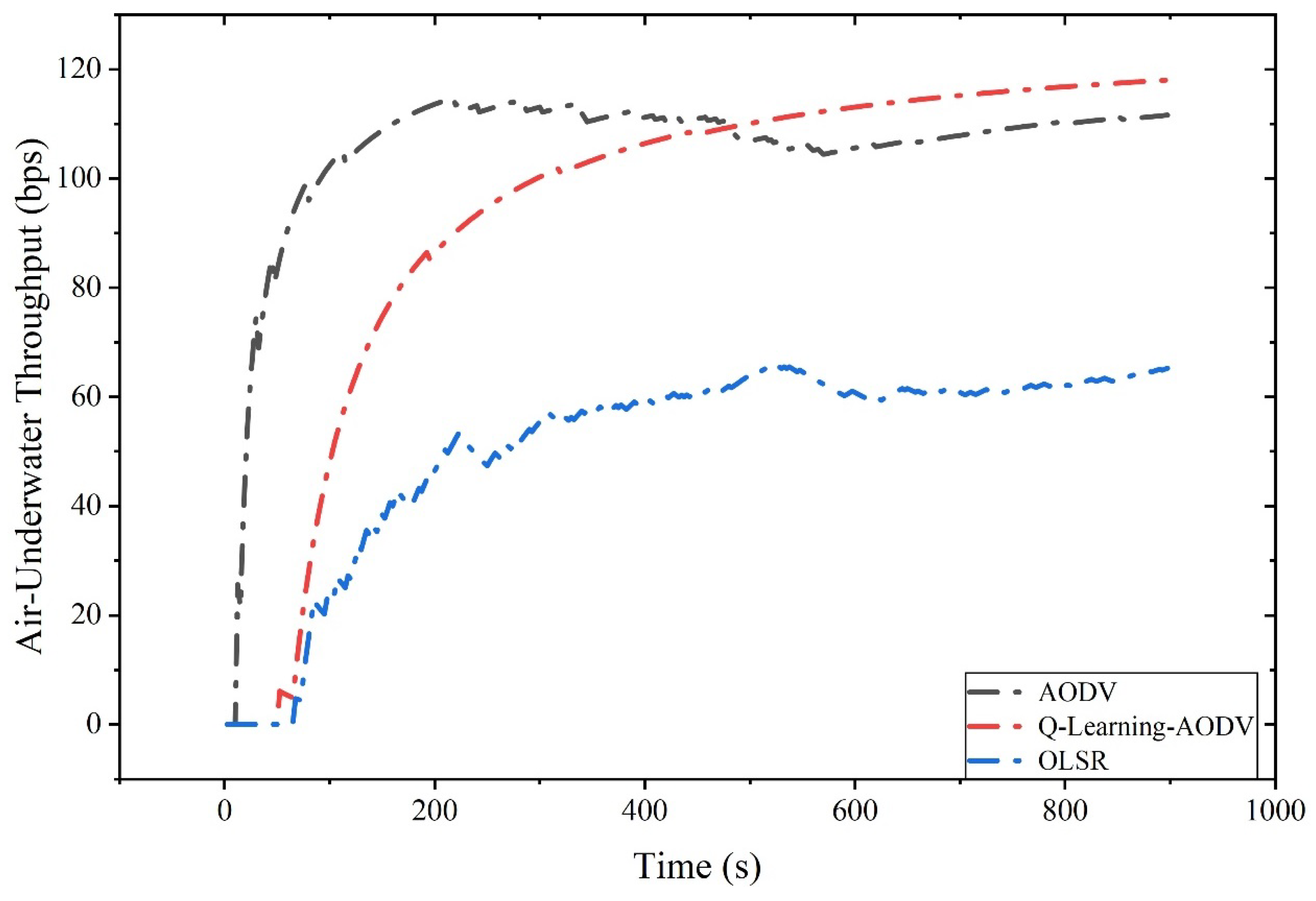
The throughput comparison for the air-to-underwater transmission scenario is shown in Figure 18, which presents the throughput performance of three protocols over time. At the initial stage, AODV achieves the highest throughput, whereas Q-Learning AODV shows relatively low throughput. As time progresses, the throughput of Q-Learning AODV gradually increases and begins to exceed that of AODV after approximately 450 s. The throughput of AODV starts to decline at around 500 s, then rises slowly, and finally stabilizes after 600 s. Although the throughput of OLSR also increases steadily after approximately 80 s, it remains clearly lower than that of the other two protocols. Since DSDV is a table-driven routing protocol that requires continuous maintenance of the global routing table, it incurs substantial routing overhead and is prone to packet collisions in underwater acoustic channels. As a result, its throughput drops to 0 in this scenario.

Overall, Q-Learning AODV exhibits more stable and efficient throughput during long-term operation. This is because the proposed protocol considers multiple reward factors and selects the path with the highest Q-value for data transmission. As a result, its routes are more stable and less prone to packet loss than those of the other three routing protocols, leading to higher overall throughput.

Delay

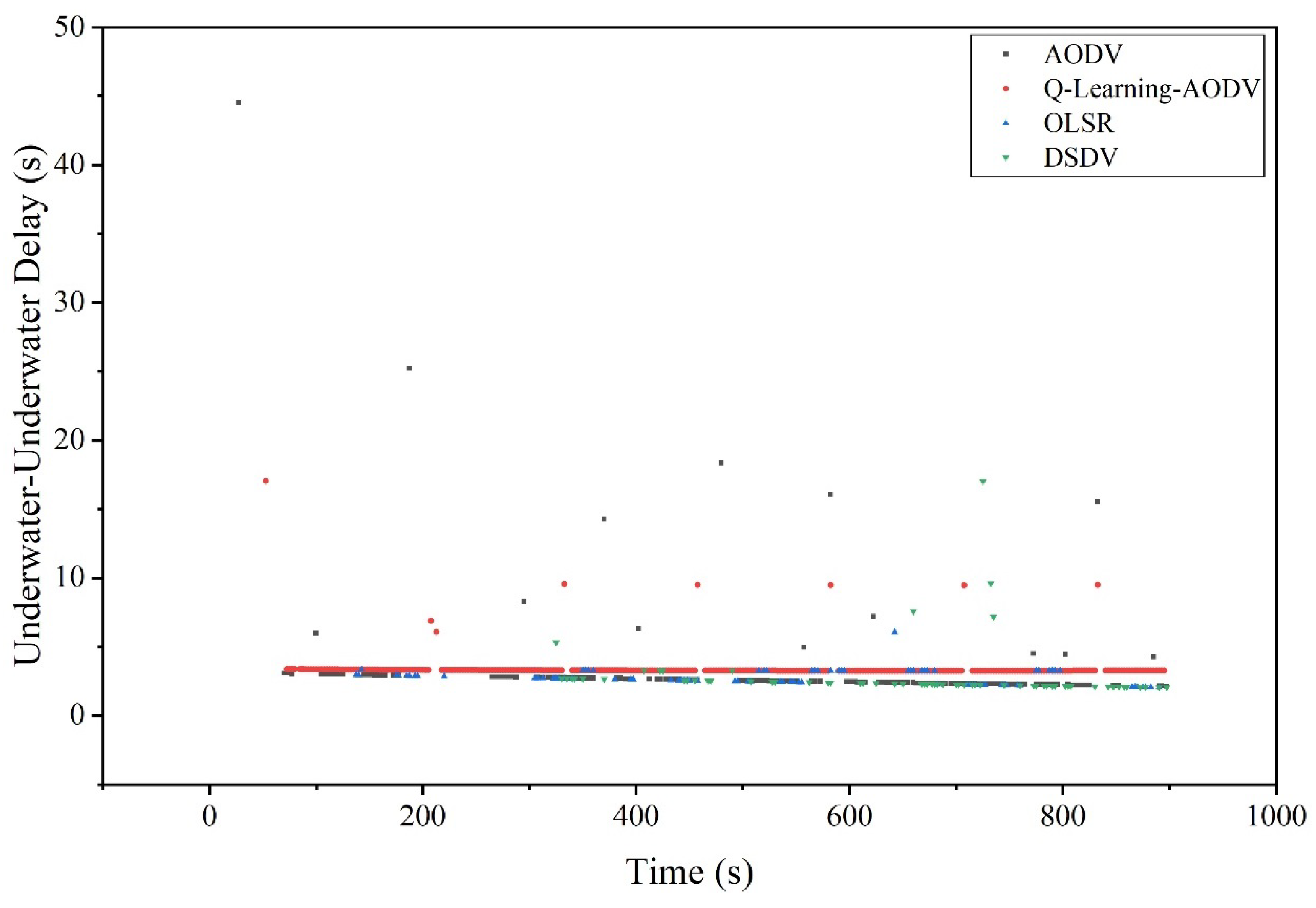
Figure 19 presents the delay comparison in the underwater-to-underwater transmission scenario, showing the delay performance of different protocols over time. It can be observed that the delays of AODV and OLSR fluctuate considerably, whereas DSDV exhibits relatively smaller delay fluctuations at certain time instants. For Q-Learning AODV, the delay decreases after approximately 400 s and gradually becomes stable overall. However, its delay remains slightly higher than that of AODV and OLSR.

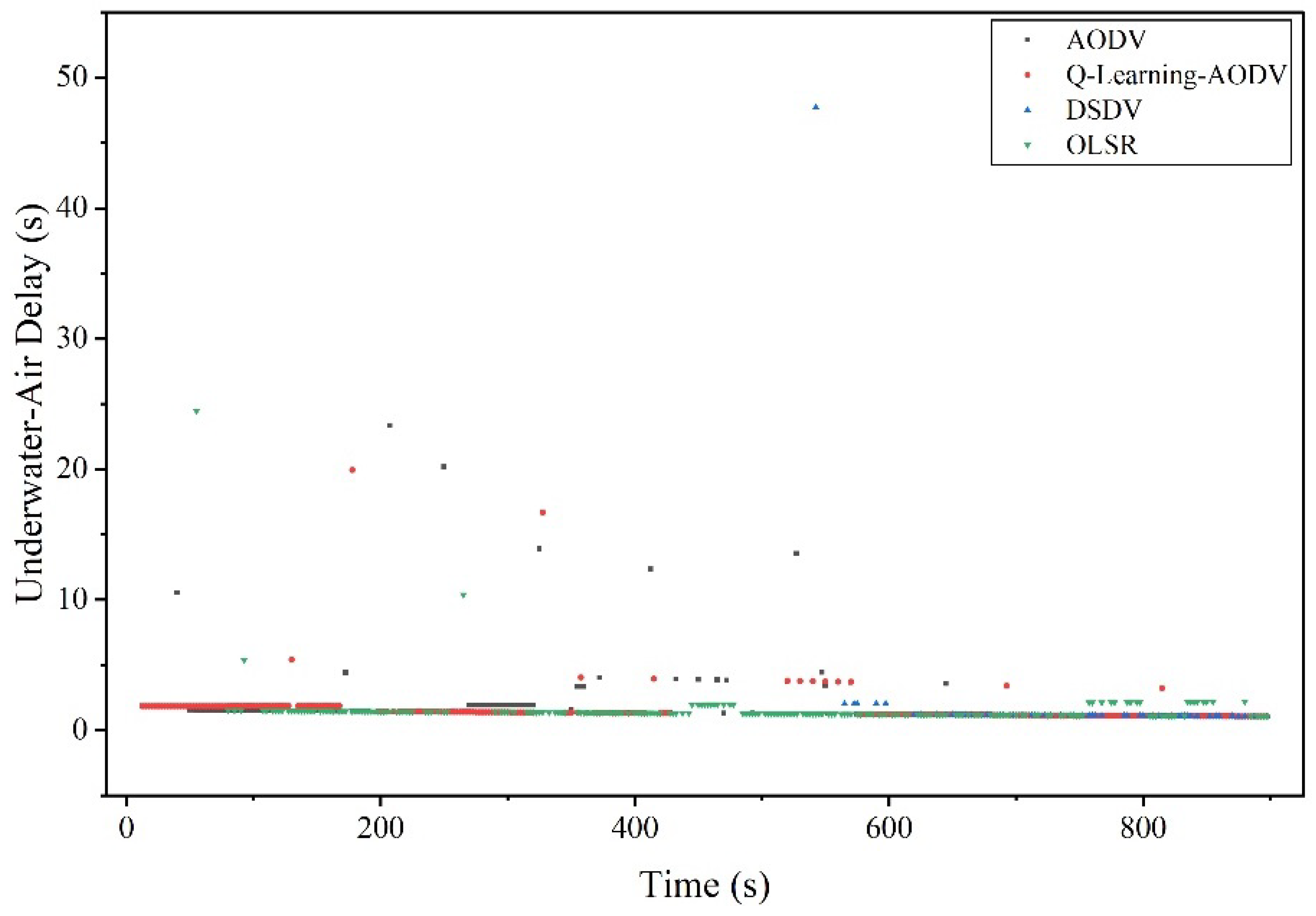
Figure 20 presents the delay comparison in the underwater-to-air transmission scenario, showing the delay performance of four protocols over time. It can be observed that, at the initial stage, AODV and OLSR exhibit relatively low delay. However, as time progresses, the delays of both AODV and OLSR fluctuate significantly and remain unstable. DSDV maintains a relatively low overall delay and outperforms AODV and OLSR in this respect. For Q-Learning AODV, the delay begins to decrease gradually after approximately 200 s and exhibits relatively stable low-delay performance during long-term operation. Overall, Q-Learning AODV achieves favorable delay performance over long-term operation, whereas the other three conventional routing protocols show relatively poor delay stability.

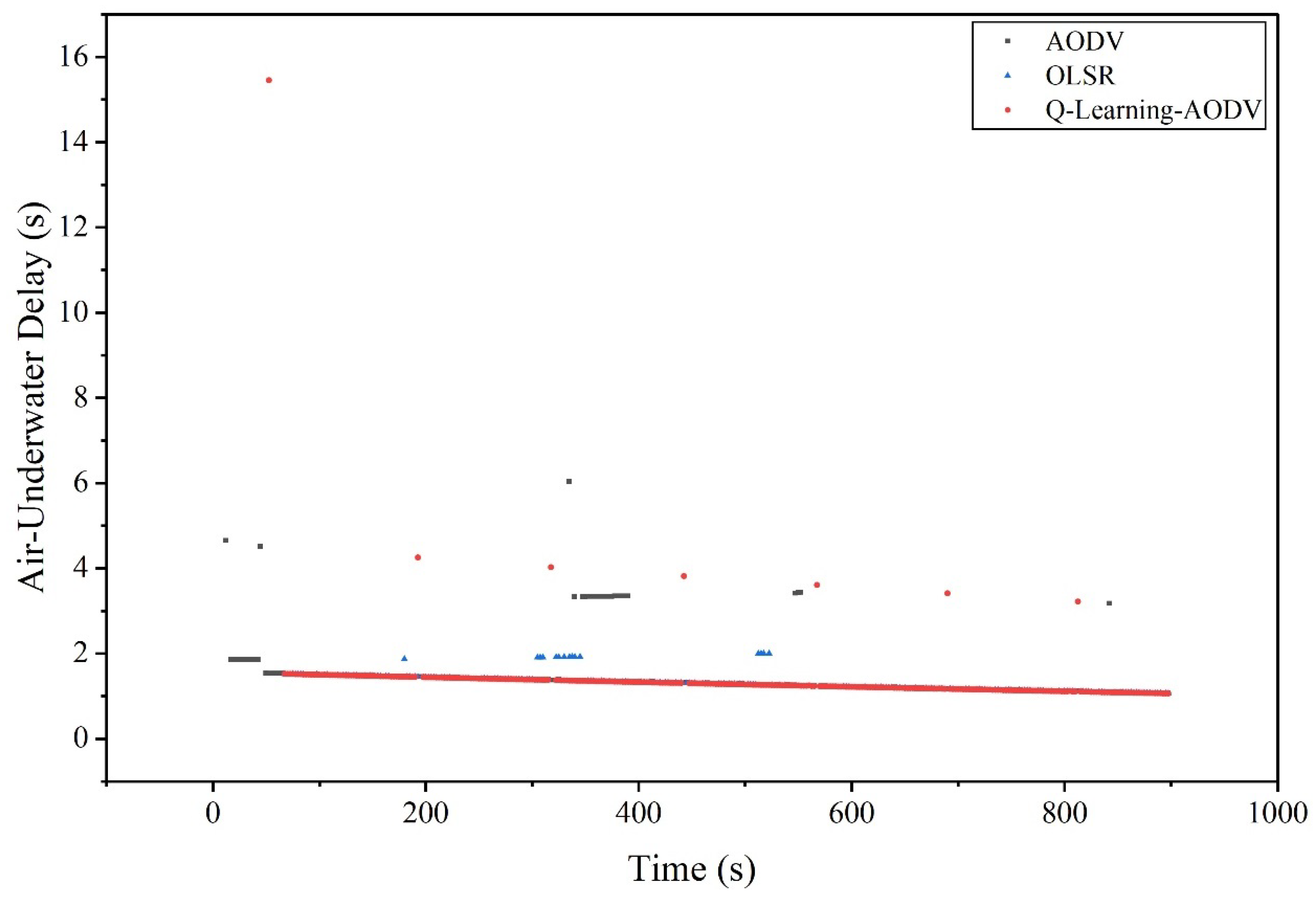
Figure 21 presents the delay comparison in the air-to-underwater transmission scenario, showing the delay performance of three protocols over time. It can be observed that, at the initial stage, AODV exhibits relatively high delay; however, as time progresses, its delay gradually decreases, although occasional fluctuations still occur. OLSR shows relatively poor stability, with more frequent occurrences of large delay, and its overall delay is slightly higher than that of the other two routing protocols. Q-Learning AODV may also exhibit occasional large delay during long-term operation. Overall, the long-term delay differences among the three protocols are relatively small. Since the packet loss rate of DSDV reaches 100% in this scenario, DSDV is not included in the delay analysis.

Taken together with

Table 7. Average delay statistics.

Average Delay (s)	Underwater-to-Underwater	Underwater-to-Air	Air-to-Underwater
Q-Learning AODV	3.44	1.64	1.37
AODV	3.25	1.49	1.83
DSDV	2.90	–	1.93
OLSR	2.77	1.33	1.56

, it can be observed that, in the air-to-underwater transmission scenario, Q-Learning AODV achieves a lower average delay than the other three conventional routing protocols. However, in the underwater-to-underwater and underwater-to-air scenarios, the delay of Q-Learning AODV is slightly higher than that of the conventional routing protocols. This is because Q-Learning AODV selects routes according to the overall link quality of a path, and the selected path is not necessarily the one with the minimum delay. As a result, its delay may be slightly higher in such scenarios. Nevertheless, this mechanism improves the stability and robustness of data transmission.

The initial communication-energy budget of the source and destination nodes is set to 90,000 J, whereas the relay nodes are initialized with 900 J. The larger source/destination budget prevents those endpoints from trivially determining the first-depletion time and allows the comparison to focus on relay-load balancing. The resulting lifetime metric is therefore a controlled routing-layer diagnostic rather than a model of complete vehicle battery endurance.

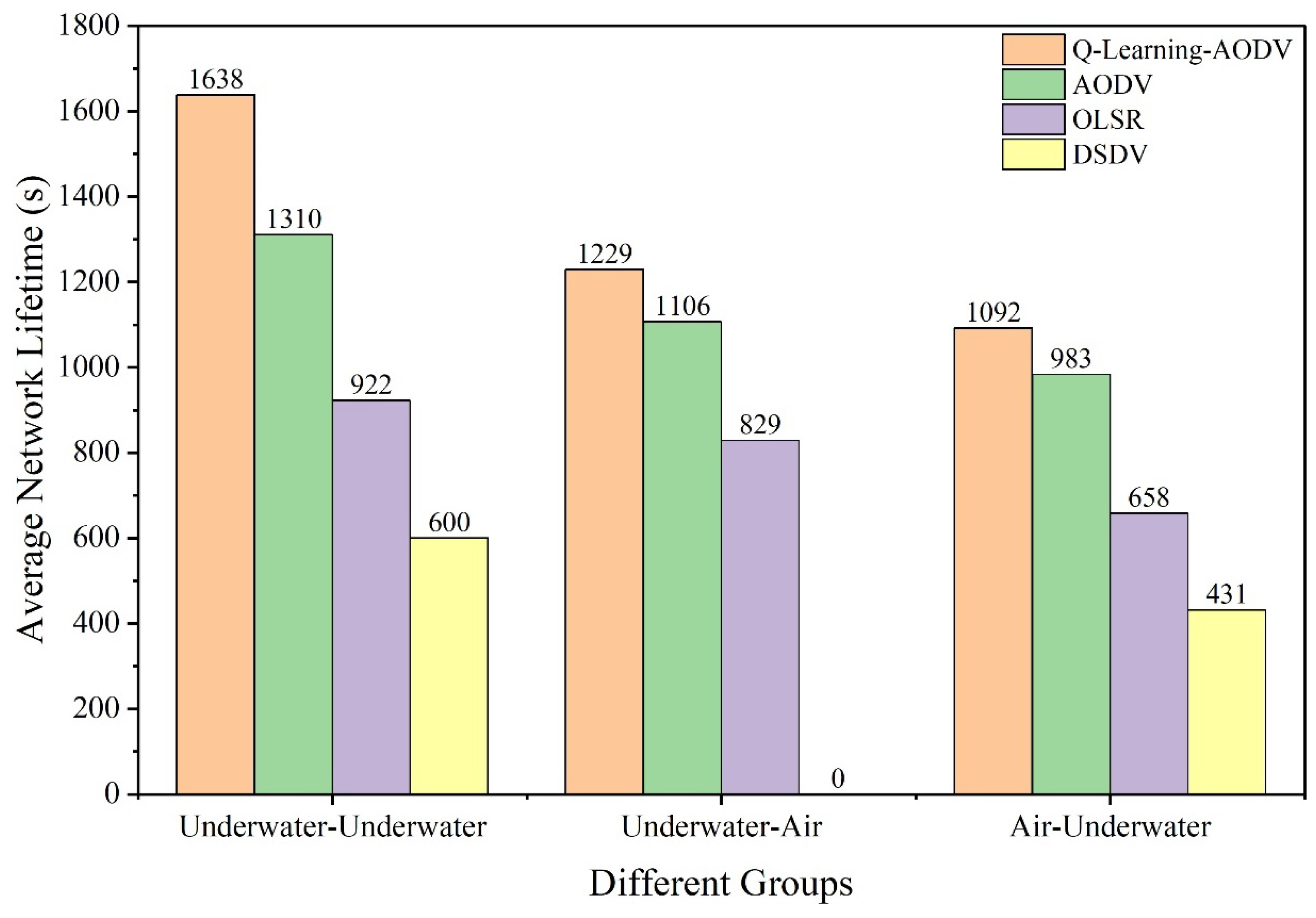
Figure 22 shows the communication-subsystem lifetime of four routing protocols under three scenarios, namely underwater-to-underwater, air-to-underwater, and underwater-to-air communications. The results indicate that Q-Learning AODV achieves the best communication-subsystem lifetime in all scenarios. This advantage is mainly attributed to its path switching mechanism and dynamic Q-value updating capability, which enable it to adapt to environmental changes and select better routes, thereby extending the communication-subsystem lifetime. As an on-demand routing protocol, AODV does not incorporate a path switching mechanism; however, it reduces control overhead through on-demand route discovery and thus also maintains a relatively long communication-subsystem lifetime in the underwater-to-underwater and air-to-underwater scenarios. By contrast, OLSR incurs higher energy consumption due to periodic route information updates, resulting in a shorter communication-subsystem lifetime than AODV. DSDV, as a table-driven protocol, requires frequent route updates and therefore introduces substantial control overhead, especially in dynamic environments. Consequently, it exhibits the shortest communication-subsystem lifetime. In particular, in the underwater-to-air scenario, DSDV fails to maintain effective communication because of severe signal attenuation and high energy consumption, leading to a communication-subsystem lifetime of zero.

Overall, the communication-subsystem lifetime results indicate that Q-Learning AODV distributes relay activity more evenly under the adopted energy model, delaying the first relay-energy depletion relative to the comparison protocols. The absolute lifetime values should not be interpreted as vehicle endurance: propulsion and navigation loads are outside the model, and the initial communication-energy budgets are deliberately chosen for routing-level comparison. Accordingly, PDR and end-to-end delay remain the primary indicators of communication performance, whereas lifetime is used only as supporting evidence of protocol-level energy balancing.

5.2.2. Performance Comparison Under Different Network Scales

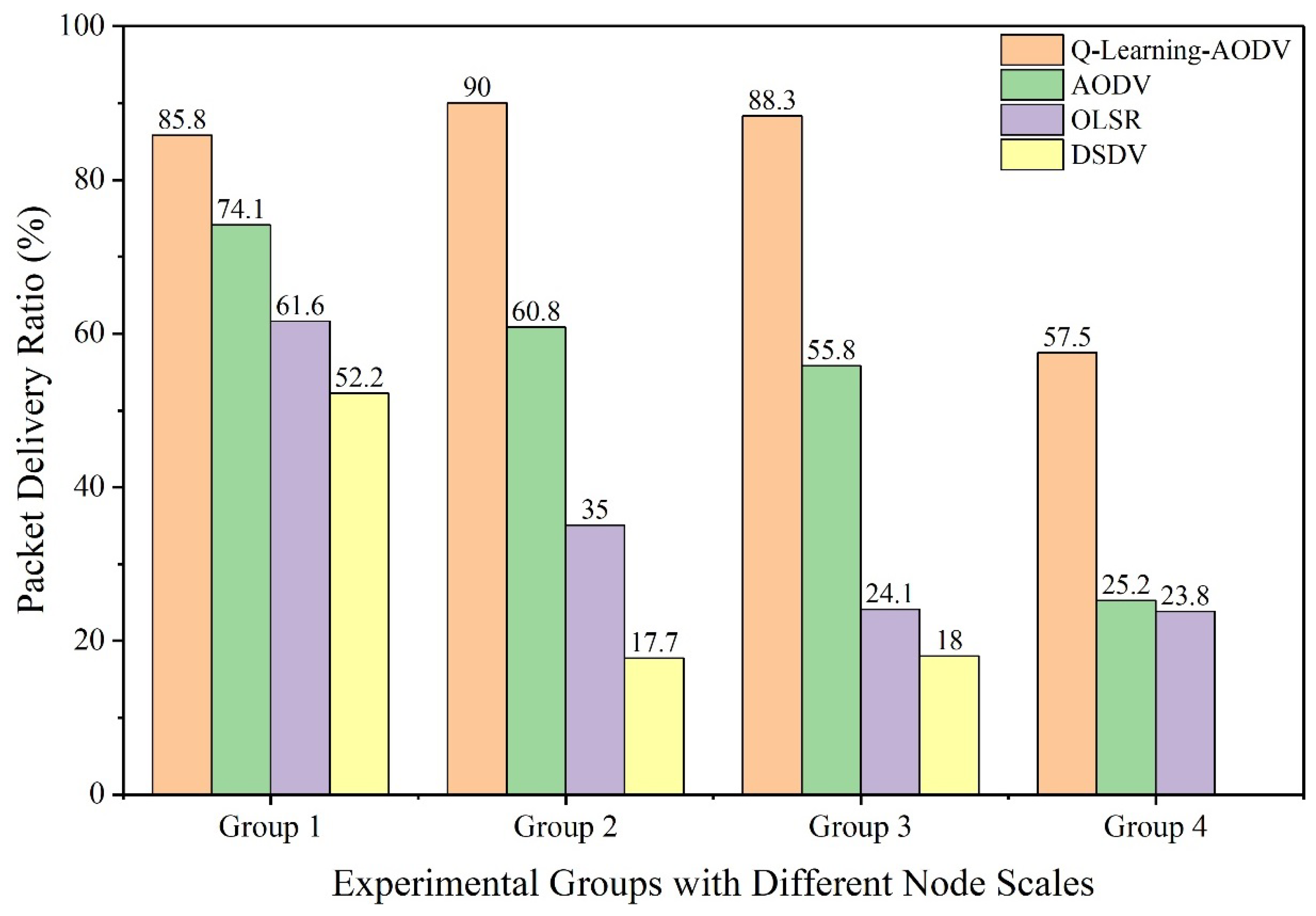
Figure 23 presents the packet delivery ratio of four routing protocols under different marine network scales. Overall, Q-Learning AODV maintains the highest delivery success rate across all scales, with its advantage being particularly pronounced at medium network scales. As the network size expands from small to medium, the packet delivery ratio remains at a high level of approximately 85.8–90.0%, with no significant degradation. Although the packet delivery ratio decreases as the network scale continues to increase, it still remains noticeably higher than that of AODV and OLSR. Among the comparison protocols, the packet delivery ratio of AODV decreases considerably as the network scale increases, whereas OLSR and DSDV exhibit even more severe degradation. In the larger tested configurations, DSDV even experiences a packet delivery ratio of 0, indicating that traditional routing mechanisms are more vulnerable to delivery degradation when multi-hop competition becomes more intense.

The main reason lies in the increased control overhead and channel contention as the network scale expands. AODV relies on RREQ flooding for route discovery, and the increase in node density and connectivity amplifies broadcast redundancy, thereby leading to packet collisions and congestion. OLSR and DSDV are proactive routing protocols that require periodic exchange of topology information or routing table updates. As the network grows larger, these control packets consume more link resources, thereby reducing the bandwidth available for effective data transmission and lowering the packet delivery ratio. By contrast, Q-Learning AODV introduces multidimensional state information and Q-value evaluation into route discovery and maintenance, making path selection more inclined to avoid heavily loaded and unstable links. As a result, it can better suppress performance degradation in medium- and the larger tested configurations, and the decline remains more controllable.

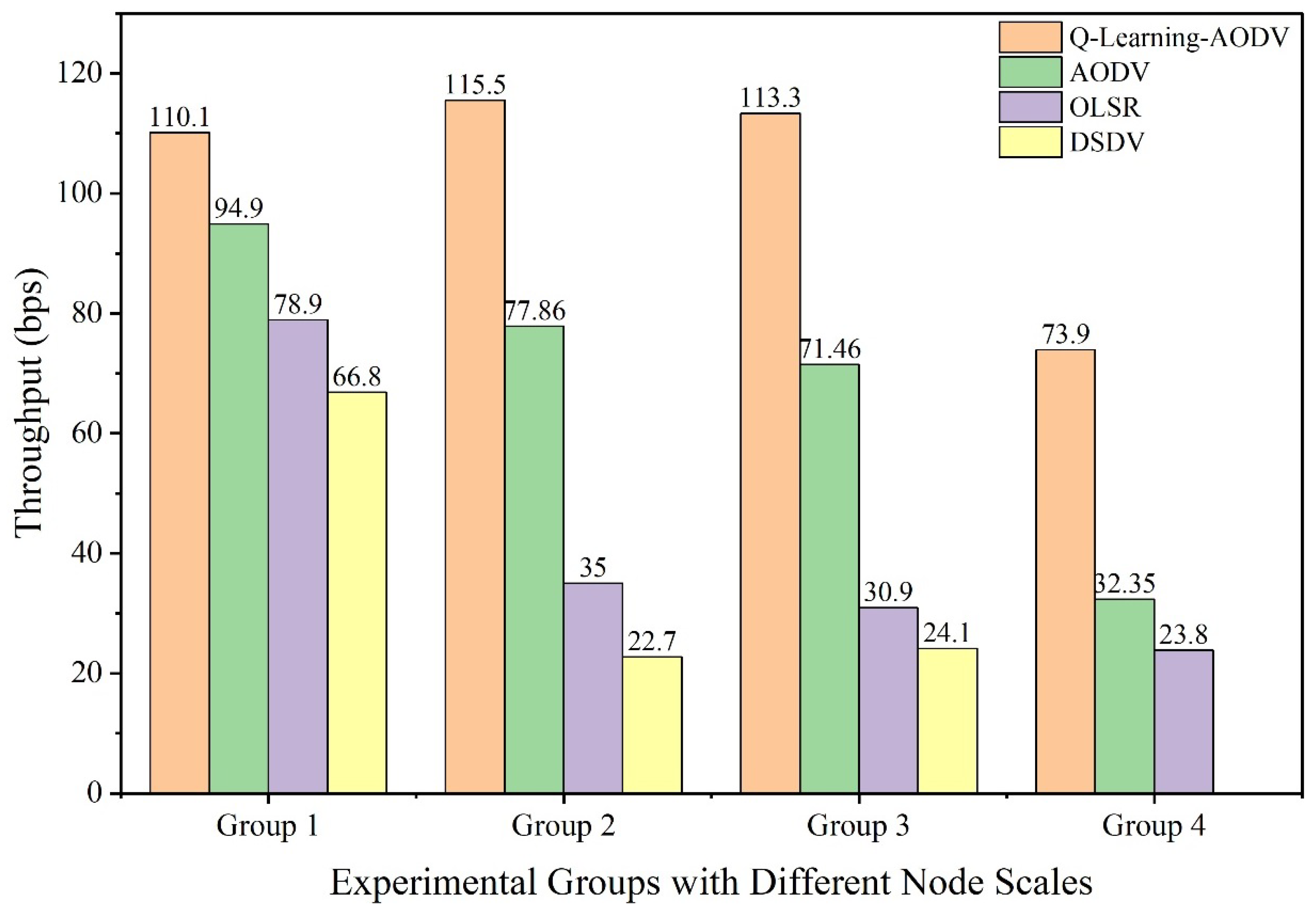
Figure 24 compares the throughput of different routing protocols under different network scales. It can be observed that Q-Learning AODV maintains a relatively high throughput under small- and medium-scale network conditions. Although its throughput decreases when the network moves to the larger tested configurations, it still remains higher than that of AODV and OLSR. The throughput of conventional routing protocols generally declines markedly as the network scale increases. In particular, OLSR and DSDV drop to relatively low levels after Group 2, indicating that when link contention intensifies, the effective payload ratio is rapidly eroded by control packet overhead and retransmissions.

The fundamental reason remains the increase in control overhead. In larger joint size/coverage configurations, RREQ flooding in AODV is more likely to trigger a broadcast storm and cause channel collisions. OLSR relies on periodic control messages such as HELLO and TC packets to maintain global topology information, whereas DSDV maintains routing consistency through periodic routing table updates. As the network expands, these overheads consume a larger share of the limited channel resources, thereby reducing throughput. In contrast, Q-Learning AODV continuously updates Q-values through the five-dimensional reward function and the link stability factor, guiding traffic toward more stable paths. In addition, the candidate set of multiple node-disjoint paths helps alleviate congestion on hotspot and bottleneck links. Therefore, it is still able to maintain higher throughput as the network scale increases.

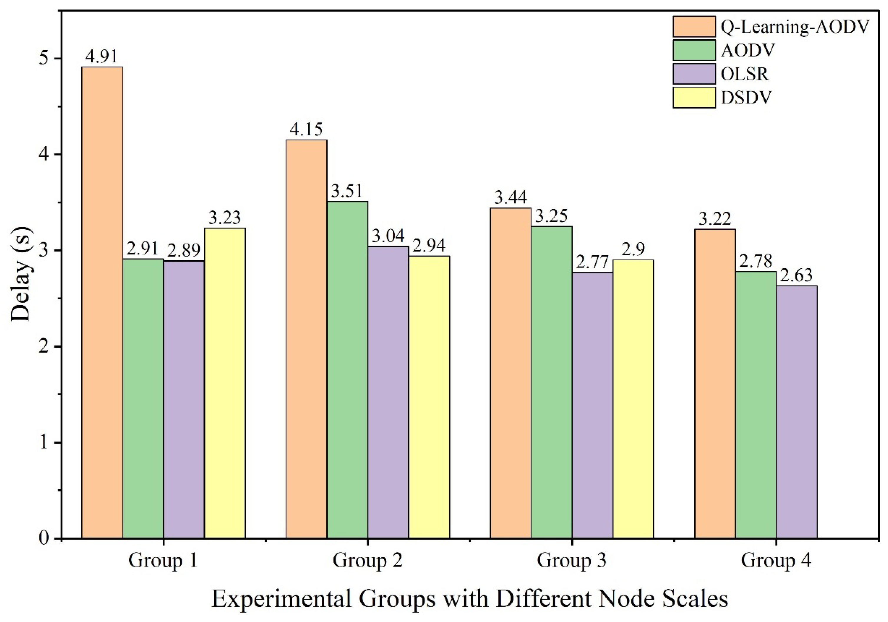
Figure 25 shows the average end-to-end delay of the same four routing protocols under different marine network scales. Unlike packet delivery ratio and throughput, Q-Learning AODV does not achieve the minimum delay. Under the small-scale network setting, its delay is approximately 4.91 s, and then gradually decreases to about 3.22 s as the network scale increases, although it still remains higher than that of AODV and OLSR overall. The delays of AODV and OLSR are generally lower and vary relatively smoothly, while DSDV lies between them under small- and medium-scale conditions.

This phenomenon reflects the trade-off between reliability and efficiency. In route selection, Q-Learning AODV tends to avoid congested or unstable links and favors more reliable paths, which may result in longer effective routes or more conservative forwarding decisions, thereby increasing end-to-end delay. By contrast, proactive routing protocols such as OLSR and DSDV maintain routing information in advance, so no additional on-demand route discovery is required during data forwarding, making it easier for them to achieve lower average delay.

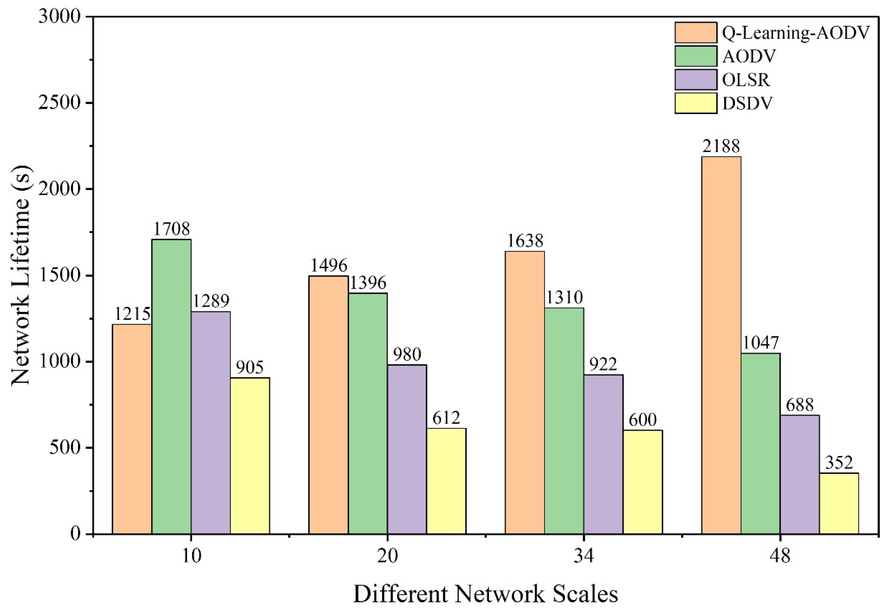
Figure 26 shows the variation in communication-subsystem lifetime of four routing protocols from Group 1 to Group 4 under different network scales. Overall, the communication-subsystem lifetime of Q-Learning AODV exhibits a clear upward trend as the network scale increases. This is because, with more nodes, the number of available paths generally increases. The Q-value updating mechanism enables path switching and load distribution during intensive forwarding, thereby preventing a small number of relay nodes from remaining in hotspot forwarding states for a long time and delaying the time at which the first node exhausts its energy. Although larger networks bring stronger contention and more collisions, the benefit brought by path diversity is generally dominant for Q-Learning AODV, so its overall communication-subsystem lifetime can still be extended.

It should be noted that, in the small-scale network of Group 1, the communication-subsystem lifetime of AODV is slightly higher than that of Q-Learning AODV. This is because, under small-scale conditions, the number of available paths is limited and the topology is relatively stable. In such cases, the exploration and update process of Q-values, together with the additional decision-maintenance overhead, may become a relative burden, whereas AODV can obtain a relatively stable forwarding path through on-demand route establishment with lower control and computational overhead, and may therefore exhibit better energy efficiency at this scale. As the network scale increases, the network lifetime of AODV, OLSR, and DSDV generally decreases. In dense networks, route discovery broadcasts in AODV are more likely to trigger collisions and retransmissions, thus increasing energy consumption. OLSR and DSDV require continuous maintenance of routing information, and the larger the network becomes, the more frequent the exchange of control packets, resulting in more pronounced additional overhead and faster degradation. Although some irregular fluctuations can be observed among different groups, Q-Learning AODV retains a relative lifetime advantage in the larger tested configurations. Because node count and coverage area vary together, this trend is interpreted as robustness to the combined stress conditions rather than as an isolated claim about network size alone.

Taken together, the four metrics indicate that Q-Learning AODV achieves the best throughput and packet delivery ratio in small-scale networks. Although its performance decreases as the network scale expands, it still remains superior to that of the other routing protocols. In terms of delay, Q-Learning AODV generally exhibits relatively higher delay under different network scales. In terms of communication-subsystem lifetime, however, Q-Learning AODV shows clear advantages over conventional routing protocols in the medium and larger tested configurations. Overall, the Q-Learning AODV routing protocol outperforms conventional routing protocols in this combined stress test. Because node count and deployment area are varied simultaneously, the observed trends reflect the joint influence of density, expected hop count, contention, and physical coverage. The curves are therefore interpreted as joint stress-response evidence rather than as an isolated scalability law. Separate fixed-area and constant-density designs would be appropriate when the objective is to decompose these individual effects.

5.2.3. Impact of Underwater Node Speed on Network Performance

Simulation experiments are conducted under different underwater node speeds, and the results are presented as follows.

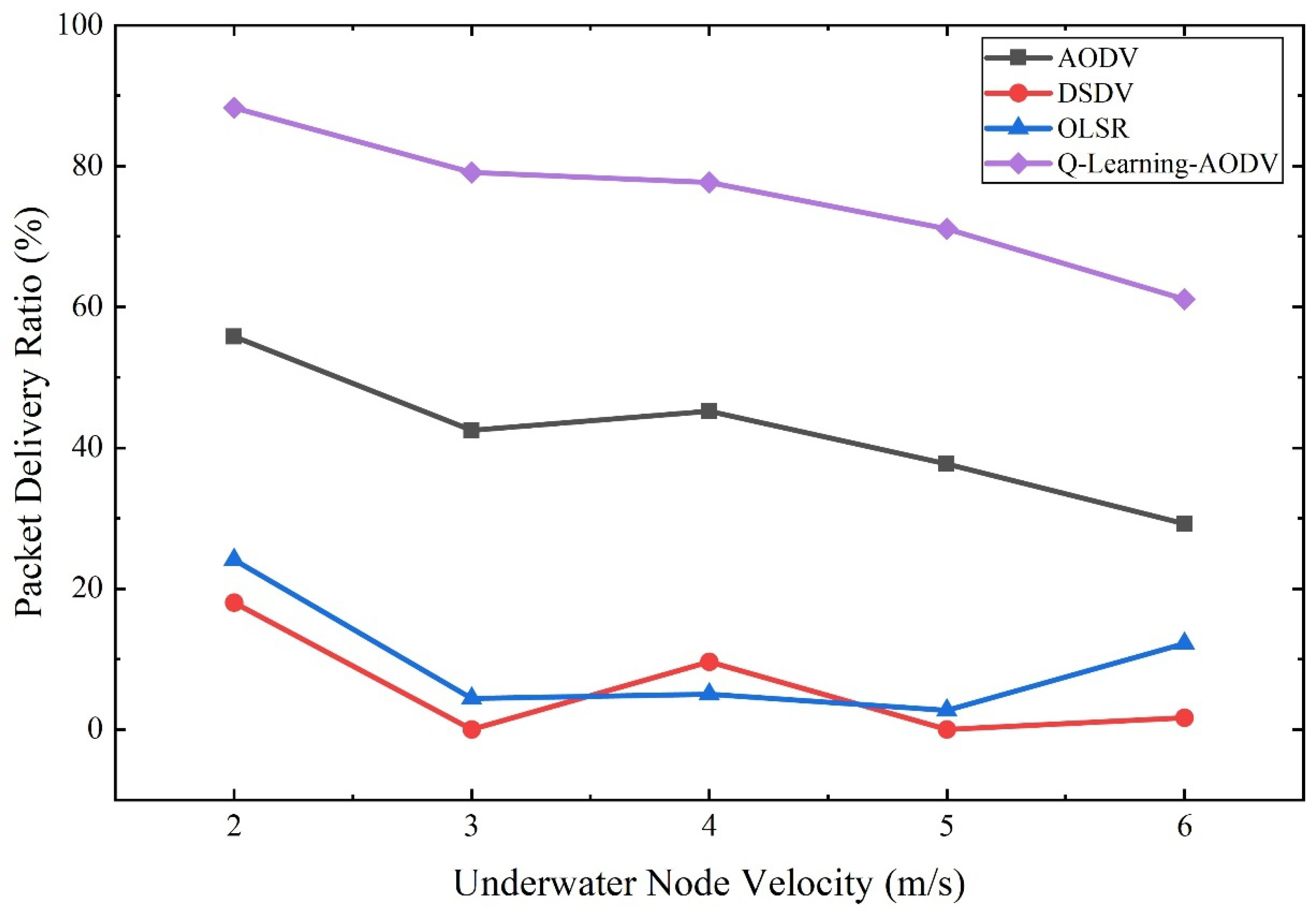
Figure 27 shows the packet delivery ratio of four routing protocols under different underwater node speeds. Q-Learning AODV achieves the best packet delivery ratio under all speed settings, followed by AODV. For both Q-Learning AODV and AODV, the packet delivery ratio exhibits a decreasing trend as node speed increases. The packet delivery ratios of AODV and its improved version remain higher than those of DSDV and OLSR. For OLSR, the packet delivery ratio is approximately 30% at 2 m/s and decreases to around 10–20% as the speed increases, resulting in relatively low overall performance. DSDV exhibits the lowest packet delivery ratio at all speed levels, and in some cases the packet delivery ratio drops to 0. Overall, Q-Learning AODV performs better than the other routing protocols under different underwater node speeds, whereas DSDV performs the worst. This is because Q-Learning AODV takes the impact of velocity difference on path stability into account and tends to select nodes with relatively small speed differences for packet forwarding, thereby improving path stability and reducing packet loss.

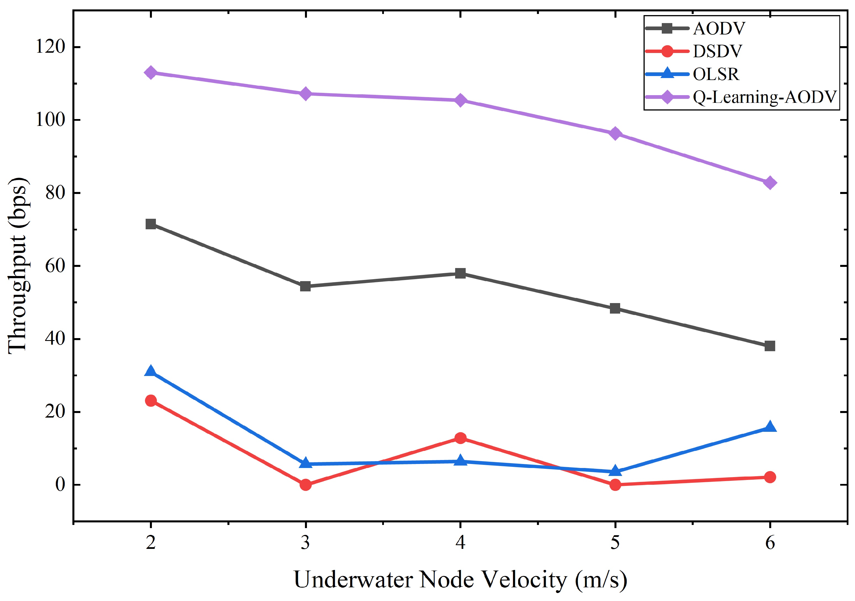
Figure 28 shows the throughput performance of the four routing protocols under different underwater node speeds. Q-Learning AODV achieves the best throughput performance under all speed settings, followed by AODV. For both Q-Learning AODV and AODV, throughput generally decreases as node speed increases. OLSR and DSDV exhibit relatively low throughput, while AODV and Q-Learning AODV maintain higher throughput than DSDV and OLSR. Overall, Q-Learning AODV achieves favorable throughput under different node speeds, with relatively high stability and a comparatively small variation range, whereas DSDV consistently exhibits the lowest throughput, including cases where throughput drops to 0. Similarly, this result can be attributed to the fact that Q-Learning AODV considers the impact of inter-node velocity difference on path stability and thus tends to select forwarding nodes with smaller speed differences, leading to more stable paths and higher throughput.

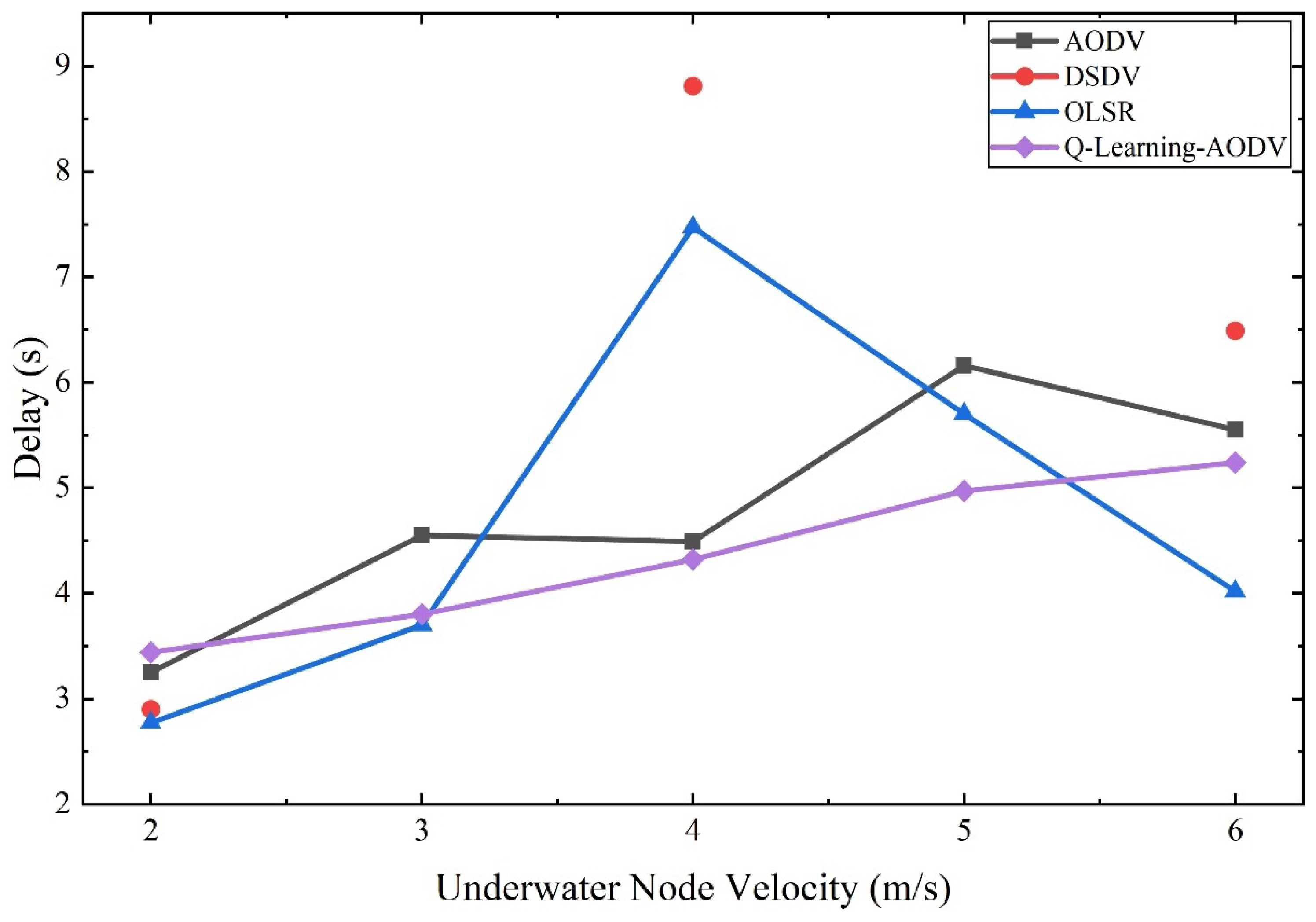
As shown in Figure 29, different protocols exhibit different delay performance as the speed of underwater nodes varies. With increasing underwater node speed, the delay of AODV and Q-Learning AODV remains relatively stable, whereas DSDV and OLSR experience larger fluctuations, indicating weaker adaptability to different node speeds. Q-Learning AODV maintains relatively low delay under different speed settings; however, when node speed increases, its delay becomes slightly higher than that of OLSR. This is because Q-Learning AODV selects routes with better overall link quality, and a higher-quality path is not necessarily the one with the minimum delay. Therefore, as node speed increases, the delay of Q-Learning AODV may become slightly higher than that of OLSR. In general, the delay of all four routing protocols increases as node speed increases. This is because higher node mobility leads to more unstable links, which causes more frequent route discoveries. During route discovery, packets may be buffered for a certain period, thereby increasing end-to-end transmission delay.

For DSDV, delay is plotted only at node speeds for which packets were successfully received; therefore, isolated red markers are shown and no line is drawn across speeds with unavailable delay values.

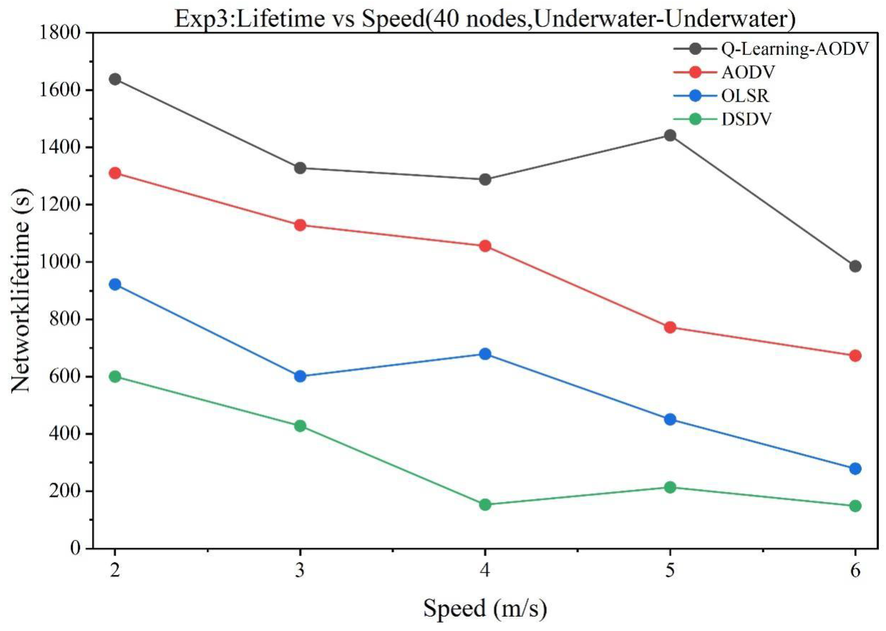
It can be seen from Figure 30 that Q-Learning AODV achieves the longest overall communication-subsystem lifetime in this underwater-to-underwater scenario with forty nodes, while still maintaining strong adaptability under different node speeds. This behavior is consistent with its use of Q-values to combine link and energy-related information and to switch among available paths when path quality degrades or node energy is consumed too quickly, thereby achieving traffic load balancing and reducing excessive consumption of hotspot relay nodes. As a result, the protocol is more likely to prolong network operation time. Specifically, when the node speed increases from 2 m/s to 4 m/s, link breakages become more frequent, and the overhead of retransmissions and route maintenance increases. Consequently, the communication-subsystem lifetime of all four protocols is generally suppressed, and Q-Learning AODV also shows a decrease. However, when the speed reaches 5 m/s, the more dynamic topology introduces more newly available paths, and the learning and switching mechanism of Q-Learning AODV can exploit these new paths to redistribute forwarding pressure, resulting in a noticeable recovery in network lifetime. When the speed further increases to 6 m/s, topology changes become too fast, the lifetime of available paths becomes shorter, and collisions as well as maintenance overhead dominate. As a result, the advantage of Q-Learning AODV is weakened, and communication-subsystem lifetime decreases significantly again. By contrast, the communication-subsystem lifetime of AODV shows an overall downward trend as speed increases, mainly due to more frequent route discoveries and broadcast contention under high mobility, which increase energy consumption. OLSR, owing to its proactive topology maintenance, is more sensitive to speed changes, and the variation of control overhead across different speed ranges causes noticeable fluctuations in its curve. DSDV, as a table-driven protocol, is prone to concentrated energy consumption due to frequent routing table updates and failures in medium- and high-speed ranges, resulting in more severe degradation. Overall, increasing node speed compresses communication-subsystem lifetime, but Q-Learning AODV, by relying on adaptive route selection and dynamic path switching, can still exploit newly available paths in certain speed ranges to achieve better energy balancing.

From the above analysis, it can be seen that different routing protocols exhibit distinct performance under different node speeds. In terms of delay, AODV and Q-Learning AODV maintain relatively stable delay under different node speeds, indicating better adaptability, whereas DSDV exhibits large delay fluctuations, reflecting insufficient stability. In terms of throughput, Q-Learning AODV performs the best and maintains the highest throughput as node speed increases, while DSDV shows the lowest throughput. In terms of communication-subsystem lifetime, Q-Learning AODV outperforms the other routing protocols. For packet delivery ratio, Q-Learning AODV also achieves a relatively high delivery rate among the four protocols, whereas DSDV remains at a low level under different speed conditions and is almost unable to satisfy communication requirements. Regarding communication-subsystem lifetime, Q-Learning AODV consistently outperforms the other routing protocols as a whole, and in medium-speed ranges it can still exploit newly available paths through Q-value learning and path switching to achieve load balancing, thereby delaying the energy depletion of critical relay nodes. In contrast, the lifetime of AODV gradually decreases due to frequent route discoveries and retransmissions, while OLSR and DSDV incur greater control overhead because of proactive maintenance and routing table updates, resulting in faster energy consumption and more pronounced lifetime degradation under highly mobile conditions.

The proposed Q-Learning AODV protocol is an improved routing protocol that introduces a reinforcement learning algorithm into the conventional AODV protocol and can dynamically adjust routing strategies according to network conditions. The protocol designs a reward mechanism that jointly considers residual node energy, network congestion, inter-node distance, velocity difference, and elevation angle, and realizes multipath routing selection through continuous Q-value updating. Experimental results show that Q-Learning AODV achieves favorable throughput, packet delivery ratio, and communication-subsystem lifetime across the tested size/coverage configurations and node-speed conditions. Although it does not always minimize delay, it maintains comparatively stable routing performance as the tested topology becomes larger or more dynamic, supporting its use as an adaptive routing option for heterogeneous marine communication scenarios.

5.3. Scope of the Evaluation and Interpretation

The evaluation is designed as a routing-level comparative study under a unified NS-3 configuration, with PDR and end-to-end delay treated as the primary performance criteria and throughput and communication-subsystem lifetime as supporting metrics. The reported evidence therefore supports relative performance conclusions for the complete Q-Learning AODV design under the stated reward, traffic, mobility, and channel settings. A statistically complete repeated-run evaluation should rerun each configuration with independent random seeds and report the sample mean together with a 95% confidence interval, $\overline{x}\pm t_{0.975,n-1}s/\sqrt{n}$. Such repeated-seed raw runs are not contained in the archived results used to generate the present figures, so confidence intervals cannot be reconstructed without rerunning the simulator. Component-level reward attribution, broad parameter robustness, and isolated density-versus-area scaling likewise require dedicated experimental designs. The underwater channel and energy results refer to the adopted routing/PHY abstraction and communication-subsystem energy boundary rather than to modem-specific multipath/Doppler behavior or complete UAV mission endurance.

6. Conclusions

This paper presented Q-Learning AODV for marine cross-medium acoustic–radio collaborative networks by coupling distributed Q-value updates with AODV route discovery/maintenance, a normalized multi-objective reward, and Q-value-ranked node-disjoint candidate paths. The revised formulation makes explicit the locally observable MDP, the sources and dissemination of routing-state variables, the link-type-dependent active reward normalization, and the additional signaling, computation, and storage cost of the learning mechanism. In the three reported communication scenarios, PDR increases from 55.8% to 88.3%, from 68.3% to 76.1%, and from 86.9% to 91.9% relative to AODV, corresponding to relative improvements of 58.2%, 11.4%, and 5.8%, respectively. End-to-end delay is not uniformly minimized, which makes PDR and delay the most informative pair of primary metrics for interpreting the routing trade-off. Throughput and communication-subsystem lifetime provide supporting evidence, with the latter reflecting routing-related communication energy only rather than complete vehicle endurance. These findings support the relative routing-level benefits of the proposed protocol under the evaluated configurations and should be interpreted within the stated PHY/channel, traffic, and communication-energy boundaries. Future work should add repeated-seed confidence intervals, broader parameter sweeps, component-level reward attribution, controlled scale decomposition, learning-based baseline implementations, and measured maritime validation.

References

1. Domingo, M.C. An overview of the internet of underwater things. J. Netw. Comput. Appl. 2012, 35, 1879–1890. [Google Scholar] [CrossRef] [Scilit]
2. Schneider, G.; Goetz, M.; Nissen, I. Design and implementation of a gateway buoy for the Underwater-IoT. In Proceedings of the 2023 IEEE 48th Conference on Local Computer Networks (LCN); IEEE: Piscataway, NJ, USA, 2023; pp. 1–6. [Google Scholar] [CrossRef] [Scilit]
3. Shang, Z.; Zhang, H. Cross-medium communication: Utilizing relay to achieve air–sea cross-medium communication technology and applications. In Proceedings of the 2nd International Conference on Internet of Things, Communication and Intelligent Technology; Lecture Notes in Electrical Engineering; Springer: Singapore, 2024; Volume 1197. [Google Scholar] [CrossRef] [Scilit]
4. Rahman, T.; Ahmad, I.; Zeb, A.; Khan, I.; Ali, G.; ElAffendi, M. Performance evaluation of routing protocols for underwater wireless sensor networks. J. Mar. Sci. Eng. 2023, 11, 38. [Google Scholar] [CrossRef] [Scilit]
5. Sathish, K.; Ravikumar, C.V.; Rajesh, A.; Pau, G. Underwater wireless sensor network performance analysis using diverse routing protocols. J. Sens. Actuator Netw. 2022, 11, 64. [Google Scholar] [CrossRef] [Scilit]
6. Li, Z.; Chitre, M.; Stojanovic, M. Underwater acoustic communications. Nat. Rev. Electr. Eng. 2024, 2, 83–95. [Google Scholar] [CrossRef] [Scilit]
7. Akyildiz, I.F.; Pompili, D.; Melodia, T. Underwater acoustic sensor networks: Research challenges. Ad Hoc Netw. 2005, 3, 257–279. [Google Scholar] [CrossRef] [Scilit]
8. Perkins, C.E.; Belding-Royer, E.M.; Das, S. Ad Hoc On-Demand Distance Vector (AODV) Routing, RFC 3561; Internet Engineering Task Force: Wilmington, DE, USA, 2003. [Google Scholar] [CrossRef] [Scilit]
9. Johnson, D.B.; Maltz, D.A. Dynamic source routing in ad hoc wireless networks. In Mobile Computing; Imielinski, T., Korth, H.F., Eds.; Kluwer Academic Publishers: Dordrecht, The Netherlands, 1996; pp. 153–181. [Google Scholar] [CrossRef] [Scilit]
10. Clausen, T.; Jacquet, P. Optimized Link State Routing Protocol (OLSR), RFC 3626; Internet Engineering Task Force: Wilmington, DE, USA, 2003. [Google Scholar] [CrossRef] [Scilit]
11. Xie, P.; Cui, J.-H.; Lao, L. VBF: Vector-based forwarding protocol for underwater sensor networks. In NETWORKING 2006; Springer: Berlin/Heidelberg, Germany, 2006. [Google Scholar] [CrossRef] [Scilit]
12. Yan, H.; Shi, Z.J.; Cui, J.-H. DBR: Depth-based routing for underwater sensor networks. In NETWORKING 2008; Springer: Berlin/Heidelberg, Germany, 2008. [Google Scholar] [CrossRef] [Scilit]
13. Basagni, S.; Petrioli, C.; Petroccia, R.; Spaccini, D. Channel-aware routing for underwater wireless networks (CARP). In Proceedings of the OCEANS 2012; IEEE: Piscataway, NJ, USA, 2012. [Google Scholar]
14. Liu, L.; Zhou, S.; Cui, J.-H. A survey on underwater acoustic sensor network routing protocols. Sensors 2016, 16, 414. [Google Scholar] [CrossRef] [Scilit] [PubMed]
15. Lyu, T.; Zhao, J.; Chen, J.; Tian, Q.; Yao, Y.; Zhang, Y.; Wei, Z.; Gulliver, T.A. Optimized AODV Routing for Cross-Medium Acoustic–Radio Collaborative Networks. J. Mar. Sci. Eng. 2026, 14, 415. [Google Scholar] [CrossRef] [Scilit]
16. Saleem, K.; Wang, L.; Bharany, S. Survey of AI-driven routing protocols in underwater acoustic networks for enhanced communication efficiency. Ocean Eng. 2024, 314, 119606. [Google Scholar] [CrossRef] [Scilit]
17. Halakarnimath, B.S.; Sutagundar, A.V. Reinforcement learning-based routing in underwater acoustic sensor networks. Wirel. Pers. Commun. 2021, 120, 401–417. [Google Scholar] [CrossRef] [Scilit]
18. Hu, T.; Fei, Y. QELAR: A machine-learning-based adaptive routing protocol for energy-efficient and lifetime-extended underwater sensor networks. IEEE Trans. Mob. Comput. 2010, 9, 796–809. [Google Scholar] [CrossRef] [Scilit]
19. Jin, Z.; Ma, Y.; Su, Y.; Li, S.; Fu, X. A Q-learning-based delay-aware routing algorithm to extend the lifetime of underwater sensor networks. Sensors 2017, 17, 1660. [Google Scholar] [CrossRef] [Scilit] [PubMed]
20. Jin, Z.; Zhao, Q.; Su, Y. RCAR: A reinforcement-learning-based routing protocol for congestion-avoided underwater acoustic sensor networks. IEEE Sens. J. 2019, 19, 10881–10891. [Google Scholar] [CrossRef] [Scilit]
21. Lu, Y.; He, R.; Chen, X.; Lin, B.; Yu, C. Energy-efficient depth-based opportunistic routing with Q-learning for underwater wireless sensor networks. Sensors 2020, 20, 1025. [Google Scholar] [CrossRef] [Scilit] [PubMed]
22. Zhou, Y.; Cao, T.; Xiang, W. Anypath routing protocol design via Q-learning for underwater sensor networks. IEEE Internet Things J. 2021, 8, 8173–8190. [Google Scholar] [CrossRef] [Scilit]
23. Chen, Y.; Zheng, K.; Fang, X.; Wan, L.; Xu, X. QMCR: A Q-learning-based multi-hop cooperative routing protocol for underwater acoustic sensor networks. China Commun. 2021, 18, 224–236. [Google Scholar] [CrossRef] [Scilit]
24. Nandyala, C.S.; Kim, H.W.; Cho, H.S. QTAR: A Q-learning-based topology-aware routing protocol for underwater wireless sensor networks. Comput. Netw. 2023, 222, 109562. [Google Scholar] [CrossRef] [Scilit]
25. Zhang, S.; Chen, H.; Xie, L. Service-aware Q-learning-based routing protocol in the underwater acoustic sensor network. Comput. Netw. 2024, 257, 110986. [Google Scholar] [CrossRef] [Scilit]
26. Li, X.; Wu, Y.; Zhu, M.; Ren, J. A Q-learning-based link-aware routing protocol for underwater wireless sensor networks. J. Mar. Sci. Eng. 2025, 13, 2374. [Google Scholar] [CrossRef] [Scilit]
27. Zhu, R.; Li, W.; Boukerche, A.; Yang, Q. Energy-Aware DRL-Based Dual-Perception Fountain Codes for Resource-Constrained UASNs. IEEE Trans. Sustain. Comput. 2026, 11, 111–122. [Google Scholar] [CrossRef] [Scilit]
28. Miuccio, L.; Riolo, S.; Bennis, M.; Panno, D. Design of a feasible wireless MAC communication protocol via multi-agent reinforcement learning. In Proceedings of the 2024 IEEE International Conference on Machine Learning for Communication and Networking (ICMLCN); IEEE: Piscataway, NJ, USA, 2024; pp. 94–100. [Google Scholar] [CrossRef] [Scilit]
29. NS-3 Project. UanPropModelThorp Class Reference. Available online: https://www.nsnam.org/doxygen/d9/d91/classns3_1_1_uan_prop_model_thorp.html (accessed on 12 August 2026).
30. Thorp, W.H. Analytic description of the low-frequency attenuation coefficient. J. Acoust. Soc. Am. 1967, 42, 270. [Google Scholar] [CrossRef] [Scilit]
31. NS-3 Project. Propagation—Model Library: FriisPropagationLossModel. Available online: https://www.nsnam.org/docs/models/html/propagation.html (accessed on 12 August 2026).
32. Al-Hourani, A.; Kandeepan, S.; Lardner, S. Optimal LAP altitude for maximum coverage. IEEE Wirel. Commun. Lett. 2014, 3, 569–572. [Google Scholar] [CrossRef] [Scilit]
33. ITU-R. Recommendation ITU-R P.676: Attenuation by Atmospheric Gases and Related Effects. Available online: https://www.itu.int/rec/R-REC-P.676 (accessed on 12 August 2026).
34. NS-3 Project. Propagation—Model Library: TwoRayGroundPropagationLossModel. Available online: https://www.nsnam.org/docs/models/html/propagation.html (accessed on 12 August 2026).
35. Khaled, Z.E.; Ajib, W.; Mcheick, H. An accurate empirical path loss model for heterogeneous fixed wireless networks below 5.8 GHz frequencies. IEEE Access 2020, 8, 182755–182775. [Google Scholar] [CrossRef] [Scilit]
36. Abramson, N. The ALOHA system—Another alternative for computer communications. In Proceedings of the Fall Joint Computer Conference; ACM: New York, NY, USA, 1970; Volume 37, pp. 281–285. [Google Scholar] [CrossRef] [Scilit]
37. IEEE Std 802.11-2016; IEEE Standard for Information Technology—Telecommunications and Information Exchange Between Systems Local and Metropolitan Area Networks—Specific Requirements—Part 11: Wireless LAN Medium Access Control (MAC) and Physical Layer (PHY) Specifications. IEEE: Piscataway, NJ, USA, 2016. [CrossRef] [Scilit]
38. Sutton, R.S.; Barto, A.G. Reinforcement Learning: An Introduction, 2nd ed.; MIT Press: Cambridge, MA, USA, 2018. [Google Scholar]
Figure 1. Topology of the acoustic–radio collaborative network. Dashed arrows denote radio links, solid arrows denote underwater acoustic links, and the blue downward arrow indicates increasing water depth.
Electronics 15 03721 g001
Figure 2. Schematic diagram of dual path reflection and water vapor absorption loss at sea.
Electronics 15 03721 g002
Figure 3. Simulation framework of the acoustic–radio collaborative network.
Electronics 15 03721 g003
Figure 4. Q-Learning interaction framework used for routing decisions.
Electronics 15 03721 g004
Figure 5. Modeling framework of the Q-Learning AODV algorithm.
Electronics 15 03721 g005
Figure 6. Schematic diagram of AODV multipath routing. S and D denote the source and destination nodes, respectively, and nodes 1–7 denote intermediate nodes; dashed black arrows indicate RREQ forwarding and solid orange arrows indicate RREP forwarding.
Electronics 15 03721 g006
Figure 7. Routing request message format.
Electronics 15 03721 g007
Figure 8. Routing response message format.
Electronics 15 03721 g008
Figure 9. HELLO message format. The ellipsis indicates additional repeated destination/Q-value entries with the same field structure.
Electronics 15 03721 g009
Figure 10. Routing table format. The ellipsis denotes additional route entries of the same structure.
Electronics 15 03721 g010
Figure 11. Route-discovery procedure at the source node.
Electronics 15 03721 g011
Figure 12. RREQ processing procedure at a receiving node.
Electronics 15 03721 g012
Figure 13. Flow charts of target-node RREQ processing and intermediate-node RREP processing. (a) Target node processing RREQ. (b) Node processing RREP.
Electronics 15 03721 g013
Figure 14. Q-value update flow chart.
Electronics 15 03721 g014
Figure 15. Topology of the simulation scenario for the acoustic–radio collaborative network.
Electronics 15 03721 g015
Figure 16. Throughput comparison for the underwater-to-underwater scenario.
Electronics 15 03721 g016
Figure 17. Throughput comparison for the underwater-to-air scenario.
Electronics 15 03721 g017
Figure 18. Throughput comparison for the air-to-underwater scenario.
Electronics 15 03721 g018
Figure 19. Underwater-underwater time delay comparison diagram.
Electronics 15 03721 g019
Figure 20. Underwater-air time delay comparison diagram.
Electronics 15 03721 g020
Figure 21. End-to-end delay comparison for the air-to-underwater scenario.
Electronics 15 03721 g021
Figure 22. Communication-subsystem lifetime comparison across the three scenarios.
Electronics 15 03721 g022
Figure 23. Comparison of packet delivery ratio under different network scales.
Electronics 15 03721 g023
Figure 24. Throughput comparison under different network scales.
Electronics 15 03721 g024
Figure 25. Delay comparison under different network scales.
Electronics 15 03721 g025
Figure 26. Communication-subsystem lifetime under different network scales.
Electronics 15 03721 g026
Figure 27. Comparison of packet delivery ratio under different underwater node speeds.
Electronics 15 03721 g027
Figure 28. Throughput comparison under different underwater node speeds.
Electronics 15 03721 g028
Figure 29. Delay comparison under different underwater node speeds.
Electronics 15 03721 g029
Figure 30. Communication-subsystem lifetime under different underwater node speeds.
Electronics 15 03721 g030