Article

Element Failure Diagnosis and Pattern Recovery for Array Antennas

1
School of Electronic and Optical Engineering, Nanjing University of Science and Technology, Nanjing 210094, China
2
Zhejiang Geespace Technology Co., Ltd., Shanghai 200233, China
*
Author to whom correspondence should be addressed.
These authors contributed equally to this work.
Electronics 2026, 15(16), 3717; https://doi.org/10.3390/electronics15163717
Submission received: 4 July 2026 / Revised: 4 August 2026 / Accepted: 18 August 2026 / Published: 19 August 2026

Abstract

To address the issues of element failures and performance degradation in antenna arrays caused by harsh outdoor environments, in this paper, we propose a neural network-based fault diagnosis method alongside an adaptive-threshold radiation pattern recovery algorithm based on the Fast Fourier Transform (FFT). For fault diagnosis, the proposed method utilizes the far-field patterns of the damaged array as input data to train and test a Convolutional Neural Network (CNN). The training dataset comprises simulated data embedded with Gaussian noise to replicate real-world conditions. Distinguishing itself from conventional neural network-based diagnostic approaches, this method innovatively applies sum-and-difference beam processing to the far-field data, effectively resolving the long-standing challenge of diagnosing symmetrical element failures while maintaining low computational complexity and achieving superior identification accuracy. Regarding performance recovery, an adaptive threshold mechanism is integrated into the traditional iterative FFT optimization algorithm. This mechanism dynamically adjusts the restoration criteria according to diverse element failure scenarios and significantly reduces the number of iterations, thereby lowering the computational overhead while enhancing the efficiency of radiation pattern recovery.

1. Introduction

Phased array antennas are widely deployed in radar, imaging, and remote sensing due to their high gain, low sidelobes, and beam-scanning capabilities [1]. However, complex operating environments and component aging often lead to element failures—for instance, a system with 8,000 units is estimated to have a 4.4% failure rate after one year of operation—which severely degrades radiation efficiency and radiation patterns [2]. Consequently, rapid fault diagnosis and performance recovery techniques are essential for maintaining the functionality of antenna systems.
In terms of fault diagnosis, technology has evolved over several decades from classical matrix operations to modern intelligent algorithms. Early research primarily utilized back-transformation and matrix methods [3], followed by signal processing techniques such as MUSIC and Matrix Pencil [4], as well as global optimization methods like Genetic Algorithms (GAs). To reduce measurement costs, diagnosis methods based on compressive sensing (CS) emerged [5]; however, their high reconstruction complexity limits real-time application. Recently, machine learning—represented by deep learning—has permeated the field [6], showing significant potential for automated feature extraction. Nevertheless, these methods generally demand high-quality training datasets, and the underlying network design significantly impacts computational complexity and hardware deployment costs [7].
Regarding performance recovery, early studies relied on numerical methods such as conjugate gradient (CG), Broyden–Fletcher–Goldfarb–Shanno (BFGS), linear programming, and constrained least squares [8]. While intuitive and computationally simple, these methods easily fall into local optima during multivariable optimization and are typically suitable only for small-scale arrays. To address complex nonlinear optimization problems, researchers introduced swarm intelligence algorithms, including Genetic Algorithms (GAs) [9], Particle Swarm Optimization (PSO), Cuckoo Search, and Differential Evolution. While these algorithms excel in global searching and multi-constraint handling, they suffer from high computational costs and slow convergence [10]. For medium-to-large arrays, iterative techniques based on the Fast Fourier Transform (FFT) leverage physical mapping for rapid pattern reconstruction. However, the recovery performance is highly dependent on the array size and the specific locations of failed elements. Defining the optimal target recovery level under varying parameters remains a critical challenge.
The contributions and innovations of this article are as follows:
(1)
We propose a physics-informed diagnostic architecture incorporating a sum-and-difference beam transformation during data preprocessing to fundamentally resolve symmetric array fault ambiguity [11]. Specifically, we leverage the physical insight that, following this transformation, symmetric faults exhibit diametrically opposite phase characteristics despite having identical amplitudes. By embedding this physical prior, our highly simplified CNN architecture can flawlessly distinguish symmetric faulty elements with an accuracy approaching 100%. This is a significant advancement over existing purely data-driven methods. Conventional approaches typically feed far-field data directly into CNNs for black-box training and attempt to force feature extraction by blindly deepening the network architecture. Consequently, these traditional networks still struggle to differentiate symmetric faults under noisy conditions, often resulting in misdiagnoses or necessitating highly precise near-field measurements.
(2)
We propose a dynamic adaptive threshold mechanism tailored specifically for pattern recovery. This mechanism is deeply coupled with the 2D FFT iteration process. It dynamically approximates the physical sidelobe level (SLL) limit of the current damaged array state. This dynamic feedback approach acts in synergy with an adaptive penalty factor to actively circumvent futile iterations. It successfully prevents ‘sidelobe rebound’ and accelerates the overall convergence speed by over 30%. The proposed method exhibits a significant advantage in time cost over heuristic optimization algorithms. Prior studies utilize adaptive thresholds predominantly for fault detection rather than pattern restoration. Conventional pattern recovery methods rely on a fixed target SLL during the iterative process. Rigidly predefined target SLLs become physically unattainable under severe array damage scenarios. Conventional fixed-threshold algorithms persistently oscillate around unreachable targets, causing non-convergence and inevitable performance degradation.
The remainder of this paper is organized as follows: In Section 2, we present the uniform linear and planar array system models, along with the proposed sum-and-difference beam far-field data preprocessing scheme. In Section 3, we detail the design of the lightweight CNN architecture and elaborate on the intelligent fault diagnosis framework. In Section 4, we introduce the iterative FFT pattern recovery method built upon the dynamic adaptive threshold and penalty step-size mechanisms. In Section 5, we provide comprehensive simulation results and quantitative comparative analyses to validate the efficacy of both algorithms. Finally, concluding remarks are presented in Section 6.

2. System Model

2.1. Array Theory

As shown in Figure 1, for a one-dimensional uniform linear array with N elements, the far-field pattern can be expressed as
F ( θ ) = n = 1 N w n e j 2 π n 1 d sin θ λ
where w n is the weight vector of the array, which is related to the steering direction of the array. d is the element spacing. θ is the angle between the signal direction and the array normal direction, and λ is the wavelength.
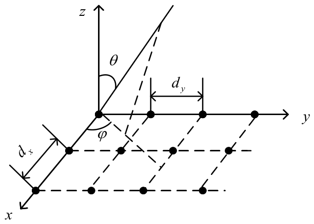
The two-dimensional planar array is shown in Figure 2. N x × N y elements are uniformly distributed along the x and y axes, and each antenna element is indexed as N x , N y . The ideal radiation pattern of the 2D planar array is expressed as follows:
F ( θ , φ ) = n = 1 N x m = 1 N y w n , m e j 2 π n 1 d x sin θ cos φ + 2 π m 1 d y sin θ sin φ λ
In the equation, d x and d y represent the antenna spacings along the x and y axes. w n , m represents the n , m complex antenna weight. θ and φ are the elevation and azimuth angles.
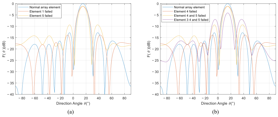
When partial element failures occur in the array, the radiation pattern gain decreases. The closer the failure location to the center, the higher the sidelobes of the pattern. Similarly, the more failed elements there are, the higher the sidelobes [12]. Taking an 8-element linear array steered towards 15° as an example, Figure 3a illustrates the impact of central versus edge element failures on the radiation pattern, while Figure 3b shows the effect of varying the number of failed elements.
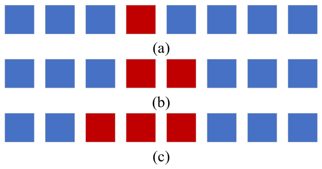
Figure 4 and Figure 5 present the schematic diagrams of the failure modes corresponding to Figure 3. Figure 4 illustrates the scenarios with different faulty element positions, where Figure 4a represents the failure of Element 1, and Figure 4b indicates the failure of Element 5. Figure 5 depicts the scenarios with different numbers of faulty elements; specifically, Figure 5a shows the failure of Element 4, Figure 5b denotes the simultaneous failure of Elements 4 and 5, and Figure 5c corresponds to the failure of Elements 3, 4, and 5.
Furthermore, the simulations in this study are conducted under standard ideal array models. We assume that the array has been well-calibrated at the factory, mitigating initial amplitude and phase errors. Additionally, complex physical non-idealities such as mutual coupling and coupled multi-element failures fundamentally alter the array manifold matrix, which represents a different modeling paradigm and falls outside the scope of this paper.

2.2. Far-Field Data Processing

Current diagnostic methods for antenna arrays can be broadly categorized into analytical mathematical methods and machine learning-based approaches. Analytical methods typically involve computationally intensive and complex mathematical derivations to achieve results [13]. In contrast, machine learning methods are highly dependent on the quality of the dataset; a well-constructed dataset can significantly simplify the neural network architecture and enhance diagnostic efficiency. Research indicates that existing neural network-based techniques are further divided into phase-less diagnostic methods and joint amplitude–phase diagnostic methods [14]. Phase-less methods generally require the array failures to be sparse; when the failure pattern violates this sparsity condition, the recovery performance degrades substantially or may fail entirely. For joint amplitude–phase diagnosis, a critical challenge remains in the detection of symmetric element failures. Existing solutions generally follow two approaches: one simply ignores such cases, which is clearly inadequate for practical applications; the other relies on inherent hardware asymmetries to distinguish symmetric elements. However, when hardware tolerances are minimal, the measured features of symmetric elements remain nearly identical, making it difficult for the neural network to identify the specific failed element and leading to erroneous outputs. To address these limitations, in this paper, we propose a novel joint amplitude–phase diagnostic method based on sum-and-difference beams. The proposed approach effectively resolves the ambiguity in symmetric element detection while offering the advantages of high precision and real-time performance.
The sum beam is synthesized through the in-phase summation of signals from individual elements within an antenna array. This processing scheme enhances the signal intensity in the main lobe direction while concurrently attenuating signals in other directions. When each array element transmits or receives signals with uniform amplitude and appropriate phase delays, a constructive focal point is established along the main lobe, typically realized by optimizing the weighting coefficients of each element. Conversely, the difference beam is generated by the anti-phase summation of signals from adjacent elements or array halves. This approach creates deep nulls in specific directions to suppress localized interference. By employing identical amplitudes but opposite phases, the signals undergo destructive interference at the null positions. This is similarly achieved via the adjustment of weighting coefficients, which, in contrast to the sum beam, utilize opposing signs to facilitate signal cancelation.
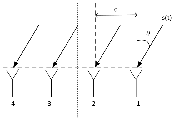
Taking a four-element uniform linear array as an illustrative example, the schematic configuration is depicted in Figure 6. In this figure, d denotes the inter-element spacing, s t represents the incident source signal, and θ is the angle of arrival relative to the array broadside. The output signals from the four antenna elements are denoted by y 1 , y 2 , y 3 , and y 4 . Assuming that the array is steered toward direction θ 0 , the weight vector w and the array manifold vector a at direction θ can be expressed as follows:
w = 1 e j 2 π d sin θ 0 λ e j 2 π 2 d sin θ 0 λ e j 2 π 3 d sin θ 0 λ
a = 1 e j 2 π d sin θ λ e j 2 π 2 d sin θ λ e j 2 π 3 d sin θ λ
The array-received signal X can be formulated as
X = s ( t ) a = s ( t ) 1   e j 2 π d sin θ λ   e j 2 π 2 d sin θ λ   e j 2 π 3 d sin θ λ
The output of each array element is given by
Y = w X = y 1 y 2 y 3 y 4 = s t   s t e j 2 π d sin θ λ e j 2 π d sin θ 0 λ   s t e j 2 π 2 d sin θ λ e j 2 π 2 d sin θ 0 λ   s t e j 2 π 3 d sin θ λ e j 2 π 3 d sin θ 0 λ
The array output is processed as follows:
y sum = y 1 + y 2 + y 3 + y 4
y difference = y 1 + y 2 y 3 y 4
The final training dataset is obtained as follows:
D amplitude = 10 log 10 1 N n = 1 N y n 2
D phase = arctan y difference y sum
In the generation of the magnitude dataset, average power is calculated and transformed into decibels for normalization. The phase dataset is derived through the sum-and-difference beam ratio followed by an inverse tangent operation. While conventional diagnostic approaches are susceptible to phase instability induced by residual carrier modulation, our methodology eliminates this interference, thereby ensuring carrier-independent phase retrieval. This approach is particularly advantageous for detecting symmetrical element failures: although such failures yield identical magnitude responses, their phase characteristics are uniquely distinguishable. Taking a four-element uniform linear array as an illustrative example, the theoretical proof of the phase feature distinguishability is formulated as follows:
R 1 = y difference 1 y sum 1 = s t e j ξ e j 2 ξ e j 3 ξ s t e j ξ + e j 2 ξ + e j 3 ξ = 1 e j ξ e j 2 ξ 1 + e j ξ + e j 2 ξ
R 4 = y difference 4 y sum 4 = s t 1 + e j ξ e j 2 ξ s t 1 + e j ξ + e j 2 ξ = 1 + e j ξ e j 2 ξ 1 + e j ξ + e j 2 ξ
Herein, R 1 represents the case where element 1 fails, R 4 denotes the case where element 4 fails, and y i signifies the failure of the i-th element, with ξ = 2 π d sin θ 0 sin θ λ .
The expression is then further simplified using Euler’s formula:
R 1 = e j ξ e j ξ 1 e j ξ e j ξ e j ξ + 1 + e j ξ = 1 2 j sin ξ 1 + 2 cos ξ
R 4 = e j ξ e j ξ + 1 e j ξ e j ξ e j ξ + 1 + e j ξ = 1 2 j sin ξ 1 + 2 cos ξ
The phase feature D phase is extracted using the standard arctangent function arctan x , defined over the principal value range π / 2 , π / 2 , by taking the ratio of the imaginary part to the real part of R . Since the real parts of R 1 and R 4 are opposite while their imaginary parts are identical, the final retrieved phase data obtained through this specific arctangent operation are precisely opposite to each other, effectively distinguishing the symmetric failure modes.
The symmetric elements of the two-dimensional array investigated in this study exhibit central symmetry with respect to the array’s geometric center. Taking Figure 2 as an example, elements (1, 1) and (4, 4) constitute a symmetric pair. The theoretical derivation for the two-dimensional array is presented below. Assuming the direction of arrival of the incident wave is θ 0 , φ 0 , we define: ξ x = 2 π d x λ sin θ cos φ sin θ 0 cos φ 0 , ξ y = 2 π d y λ sin θ sin φ sin θ 0 sin φ 0 . Therefore, the receiving response of an arbitrary element is given by:
y n , m = e j n 1 ξ x + m 1 ξ y
Since the geometric center of the 4 × 4 array is located at n c = 2.5 and m c = 2.5 , the relative center indices are defined as:
n ˜ = n 2.5
m ˜ = m 2.5
Extracting the common central phase factor of the array, Φ c :
Φ c = 1.5 ξ x + 1.5 ξ y
Consequently, the receiving response of an arbitrary element can be simplified to:
y n , m = e j Φ c e j n ˜ ξ x + m ˜ ξ y
Under normal operating conditions, the sum and difference beams can be simplified as follows:
y sum = e j Φ c n = 1 4 m = 1 4 e j n ˜ ξ x + m ˜ ξ y = e j Φ c A
y difference = e j Φ c m = 1 4 e j m ˜ ξ y n = 1 2 e j n ˜ ξ x n = 3 4 e j n ˜ ξ x = e j Φ c j C
Based on Euler’s formula, the imaginary components in y sum perfectly cancel out, resulting in a purely real summation value, denoted as A . Similarly, the intermediate summation in y difference yields a purely real number C , while the final subtracted term produces a purely imaginary number j .
When element (1,1) fails, we have:
y sum 1 , 1 = y sum y 1 , 1 = e j Φ c A cos Φ c + j sin Φ c
y difference 1 , 1 = y difference y 1 , 1 = e j Φ c j C cos Φ c + j sin Φ c
R 1 , 1 = y difference 1 , 1 y sum 1 , 1 = cos Φ c j sin Φ c C A cos Φ c j sin Φ c
When element (4,4) fails, we obtain:
y sum 4 , 4 = y sum y 4 , 4 = e j Φ c A cos Φ c j sin Φ c
y difference 4 , 4 = y difference + y 4 , 4 = e j Φ c j C + cos Φ c j sin Φ c
R 4 , 4 = y difference 4 , 4 y sum 4 , 4 = cos Φ c j sin Φ c C A cos Φ c + j sin Φ c
A direct comparison reveals that R 4 , 4 = R 1 , 1 ¯ . This demonstrates that their real parts are opposite while their imaginary parts are identical. Consequently, the final extracted phase data are also exactly opposite. This conclusion is consistent with that of the one-dimensional array scenario.

3. Antenna Array Element Failure Diagnosis Using Neural Networks

The core strengths of CNNs reside in their specialized spatial feature processing capabilities and efficient parameter utilization [15]. By emulating the biological visual system, CNNs employ convolutional kernels for local scanning, where the local connectivity allows the network to focus on essential information within spatial neighborhoods. This facilitates the precise extraction of local features such as textures, edges, and shapes [16]. Unlike traditional methodologies, CNNs automate the feature extraction process through backpropagation, eliminating the need for exhaustive manual feature engineering. Furthermore, the weight-sharing mechanism is fundamental to reducing computational complexity; the reuse of kernels across the input space significantly minimizes the number of learnable parameters, thereby mitigating overfitting and enabling the processing of high-resolution data. In conjunction with pooling operations, CNNs achieve robust translation invariance, maintaining consistent recognition regardless of the target’s position. This hierarchical learning paradigm—transitioning from low-level geometric primitives to high-level semantic abstractions—endows CNNs with superior generalization and robustness for grid-structured data [17].

3.1. Proposed CNN Architecture

In the proposed method, far-field data are fed into a CNN to predict the faulty elements of the antenna array. Given the practical challenges of collecting large-scale training datasets, simulated data generated according to the methodology detailed in Section 2 are utilized for model training.
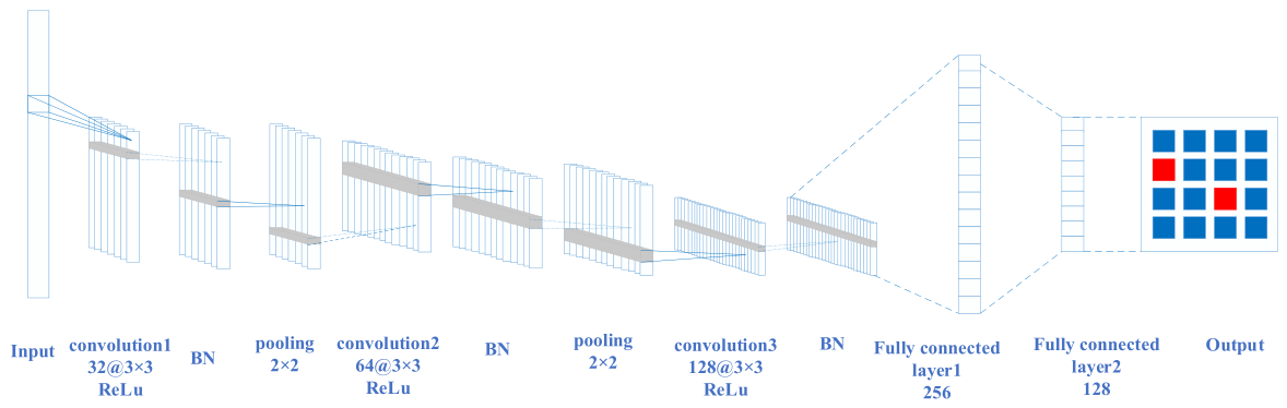
The internal architecture of the model employed in this study is illustrated in Figure 7, with detailed hyperparameters summarized in Table 1. The input to the network is an H × W matrix. In the far-field data simulation, spatial sampling is performed at 8° intervals. Both the elevation angle θ and the azimuth angle φ range from −90° to 90°, resulting in input data dimensions of 23 × 26 . Specifically, the left 23 × 23 partition represents the amplitude data, while the right 23 × 23 partition contains the phase data.
The front-end of the network comprises three convolutional layers dedicated to feature extraction. These layers utilize 32, 64, and 128 filters, respectively, with a uniform kernel size of 3 × 3 and the ReLU activation function. Batch normalization and pooling layers are integrated following the first two convolutional layers; the former is employed to accelerate convergence. A 2 × 2 pooling window is used to facilitate dimensionality reduction and minimize the computational complexity of the network. The output of the third convolutional layer is fed into a flattening layer, which transforms 2D feature maps into a 1D vector for direct connection to the back-end. The back-end consists of two fully connected (FC) layers with 256 and 128 neurons, respectively, both employing ReLU activation. During the training phase, a dropout rate of 30% is applied to the FC layers, where neurons are randomly deactivated to prevent overfitting and enhance the model’s generalization capability.
The specific architecture detailed in Table 1 was deliberately designed based on stringent selection criteria and performance trade-offs. Conventional deep learning approaches typically feed far-field data directly into CNNs for black-box training and attempt to force feature extraction by blindly deepening the network architecture. However, because our method leverages a strong physical prior via sum-and-difference beam preprocessing, a highly simplified CNN architecture is sufficient. The primary selection criterion for the network depth—strictly comprising the aforementioned three convolutional layers—is to ensure efficient hierarchical feature extraction while avoiding the severe overfitting associated with redundant parameterization. Furthermore, the 3 × 3 kernel size is specifically chosen to capture local spatial correlations within the far-field data while strictly minimizing the number of learnable parameters. Compared to conventional, heavier deep-learning architectures, this streamlined design offers significant advantages in terms of performance parameters. By drastically minimizing computational complexity through efficient parameter utilization, the proposed architecture avoids the high hardware deployment costs typical of excessively deep networks. This design strikes an optimal balance: it maintains an extremely low memory footprint suitable for real-time array diagnosis while achieving superior identification performance, consistently yielding an exact-match accuracy approaching 100%.
The final diagnostic performance is demonstrated on a 4 × 4 planar array. The network output is represented as a 1 × 16 binary vector, where ‘0’ and ‘1’ denote healthy and faulty elements, respectively. To evaluate the model’s effectiveness, several metrics are employed: area under the curve (AUC), precision, recall, micro-averaged F1-score, and exact-match accuracy. Specifically, the AUC characterizes the model’s intrinsic performance under conditions of class imbalance; a model is considered viable when AUC > 0.8. Precision measures the proportion of true failures among all predicted faulty elements, while recall indicates the ratio of successfully identified failures to the total number of actual faulty elements. The micro-averaged F 1 score is defined as the harmonic mean of precision and recall, with the formulation provided below. Lastly, the exact-match accuracy is a stringent metric that requires the predicted failure state to be identical to the ground truth for the entire array.
F 1 score = 2 × P × R P + R
Due to the diversity of fault scenarios, using one-hot encoding leads to excessive memory overhead. Therefore, in this study, a multi-hot encoding scheme is adopted. The output layer utilizes the Sigmoid activation function. Regarding the loss function, experimental results show that the performance of Focal Binary Cross-Entropy (Focal-BCE) is comparable to that of traditional BCE; thus, traditional BCE is employed in this paper to train the network, with the expression J :
J = 1 N i = 1 N y i log p + 1 y i log 1 p
During the model training phase, the Adam optimizer is utilized with a batch size of 32 and an initial learning rate of 0.001. The training is set for a maximum of 100 epochs. To ensure optimal convergence and robust performance, a comprehensive callback strategy is implemented. Specifically, an early stopping mechanism terminates the training if the AUC on the validation set fails to improve for 15 consecutive epochs, thereby preventing the model from converging to a falsely high accuracy caused by all-zero predictions. Additionally, a model checkpoint mechanism is employed to monitor the validation AUC and save the optimal model weights. Furthermore, a learning rate scheduler dynamically halves the learning rate if the validation loss plateaus for 5 consecutive epochs (with a minimum learning rate of 1 × 10⁻⁶), preventing the model from oscillating around local minima.

3.2. Array Element Failure Diagnosis Using CNN

This study simulates a far-field measurement environment for antenna arrays. In the far-field region, the radiation patterns of an array containing faulty elements exhibit significant deviations compared to those of an intact array. By processing radiation data—which inherently contains failure signatures—through CNN, the positions of faulty elements can be accurately diagnosed. The proposed diagnostic framework is executed in three distinct stages.
Step 1: Far-Field Data Acquisition. A signal source is positioned in the far-field, and the received signals of the array are recorded to construct the diagnostic dataset. To emulate practical testing conditions and comprehensively validate the network’s capabilities, the data is corrupted with mixed Gaussian noise, with the Signal-to-Noise Ratio (SNR) set to 30 dB. Furthermore, to rigorously assess the algorithm’s tolerance to time-varying environmental drifts and inherent physical hardware limitations, non-ideal factors including random amplitude-phase errors (uniformly distributed within ±0.5 dB and ±5°, respectively) and weak mutual coupling effects (modeled with a −20 dB coupling coefficient) are explicitly incorporated into the signal model. It is crucial to emphasize that in the proposed method, the phase data serves as the primary diagnostic feature. As mathematically formulated in Section 2.2, the extracted phase responses are intrinsically decoupled from the SNR, being solely dependent on the physical geometry of the array. To ensure that the network sufficiently learns all failure characteristics, a massive dataset consisting of 209,100 samples was generated, exhaustively covering various random symmetric and asymmetric failure combinations. This exhaustive physical simulation inherently provides extensive data diversity, acting as a robust data augmentation strategy to prevent model overfitting.
Step 2: CNN Model Training and Validation. The total generated dataset is partitioned into a training set of 146,370 samples (70%), a validation set of 31,365 samples (15%), and a testing set of 31,365 samples (15%). The model is subsequently trained utilizing the specific hyperparameters and callback strategies detailed in Section 3.1.
Step 3: Failure Diagnosis. Leveraging the trained CNN architecture, faulty elements within the array are identified with high accuracy. The final output provides the specific indices corresponding to the failed elements.

4. Adaptive-Threshold Pattern Recovery Based on FFT

Compared with conventional optimization techniques, phased array radiation pattern recovery based on the Fast Fourier Transform (FFT) offers revolutionary advantages, the core of which lies in its ingenious exploitation of the inherent mathematical mapping between the physical array aperture and the far-field pattern [18]. For a planar array with uniform spacing, an exact inverse Fourier transform relationship natively exists between the array factor and the element excitations. Capitalizing on this principle, the FFT-based method synchronously computes and updates the excitation coefficients of all array elements in a single step by alternating between forward and inverse two-dimensional FFTs between the aperture and far-field domains. This mechanism completely breaks free from the constraints of sequential variable-by-variable optimization, imparting exceptional computational efficiency to the algorithm [19].
The superiority of the FFT method over traditional optimization approaches becomes particularly pronounced when handling ultra-large-scale arrays. Traditional optimization methods heavily rely on cost functions, requiring continuous error evaluation and tedious hyperparameter tuning; consequently, they are prone to the curse of ‘dimensionality’ when applied to large planar arrays [20]. In contrast, the execution time of the FFT synthesis algorithm is virtually decoupled from the physical scale of the array, being constrained almost exclusively by the stringency of the target sidelobe level (SLL). Even for ultra-large planar arrays comprising tens of thousands of elements, this method typically achieves synthesis within a few to twenty minutes. Furthermore, the FFT-based iterative approach comprehensively outperforms traditional algorithms in terms of both algorithmic robustness and engineering practicability. While the optimization paths of conventional methods are highly susceptible to local optima and suffer from convoluted logic, the FFT method features an exceptionally streamlined logic. It eliminates the need for constructing intricate optimization models or iteratively tuning hyperparameters. In fact, its core modules can be implemented in just a few lines of code, resolving the computational bottlenecks of traditional optimization algorithms through minimalist logic and maximum efficiency.

4.1. FFT-Based Pattern Synthesis

As mentioned previously, the far-field radiation pattern of an N-element uniform linear array can be expressed as follows:
F ( θ ) = n = 0 N 1 w n e j 2 π n d sin ( θ ) λ
The M-point Discrete Fourier Transform (DFT) is given by:
X m = m = 0 M 1 x m e j 2 π M k m , 0 m M 1
Applying spectrum centralization to this equation yields the following transform:
X m = m = 0 M 1 x m e j 2 π M k m , M 2 m M 2 1
Comparing the two equations above reveals that they share an essentially identical form, which implies that the array radiation pattern can be obtained by applying the DFT to the array weights. By letting u = sin θ , the corresponding angle for each Fourier sampling point can be calculated as follows:
j 2 π λ n d u = j 2 π M k m
θ FFT = arcsin u = arcsin m λ M d
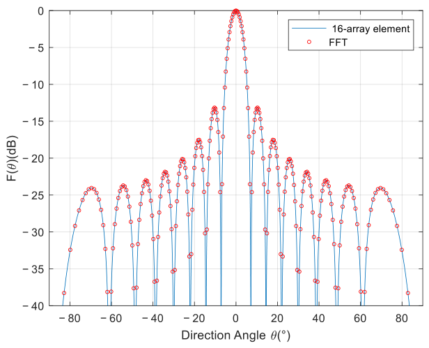
where m denotes the m-th sampling point of u , = λ M d is the sampling interval, and θ FFT represents the angle corresponding to the m-th point. Figure 8 illustrates the comparison between the FFT-based pattern synthesis and the conventional array factor method for a 16-element array. It can be observed that the FFT points perfectly coincide with the original radiation pattern.

4.2. Adaptive Step-Size and Threshold Pattern Recovery

Although FFT-based pattern recovery algorithms are capable of sidelobe suppression, they conventionally rely on a fixed threshold. However, the ultimate recovery performance varies significantly depending on the array’s element count, the specific locations of element failures, and the overall array geometry. Consequently, employing a fixed threshold for pattern restoration frequently fails to meet the predefined SLL. This discrepancy does not necessarily indicate a failure of the algorithm; rather, it largely stems from the physical inability of the degraded array to meet such stringent requirements. Conversely, even in scenarios where the target SLL is successfully achieved, the array might still possess the potential for superior performance, indicating that a fixed threshold can lead to an underutilization of the array’s remaining capabilities.
To address this, the adaptive-threshold pattern recovery method proposed in this paper resolves the challenge of dynamic threshold updating. The algorithm adaptively adjusts the threshold according to the specific conditions of the damaged array, enabling it to closely approximate the theoretical optimal recovery performance. If the initially specified target SLL is physically achievable by the array, the algorithm will execute the suppression exactly at that level. Furthermore, the proposed method optimizes the sidelobe suppression mechanism to facilitate faster iteration convergence, thereby significantly reducing the computational time overhead of the algorithm.
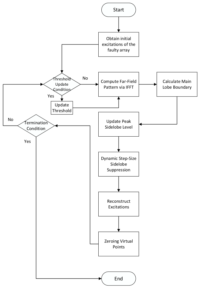
The adaptive-threshold pattern recovery is formulated on the basis of FFT-based pattern synthesis. The restoration method proposed in this paper specifically targets amplitude weighting, and its overall flowchart is illustrated in Figure 9. The algorithm utilizes the excitations of the faulty array as the initial weight parameters. Prior to calculating the radiation pattern, a threshold update condition is evaluated. When the optimal SLL ceases to change over a predefined number of iterations, the algorithm restores the optimal weights and updates the threshold. The threshold update equation is given by:
T new = T old + ( S best T old ) × 0.5
where T new is the updated threshold, T old is the original threshold, and S best is the best achieved sidelobe suppression result. The condition for threshold updating is governed by the variable m iter . The threshold update mechanism is activated when m iter = 50 , at which point the iteration termination variable r is also updated. The procedure for updating m iter will be discussed later in this section.
When calculating the radiation pattern, applying either the Fourier transform or the inverse Fourier transform yields identical results; this paper adopts the inverse Fourier transform. After performing the IFFT on the iteration variable w iter , a spectrum centralization operation is applied to the result to obtain F shift . The phase data at each point, denoted as F phase , along with the current maximum amplitude F max , are recorded to facilitate the subsequent excitation retrieval process. Finally, F shift is expressed on a logarithmic amplitude scale.
During the iteration process, to suppress the sidelobes to the greatest extent possible while preserving the main lobe performance, the main beamwidth must be constrained. Here, the main lobe region of the faulty pattern is utilized as the reference. The main lobe boundaries of a one-dimensional linear array consist of two vertical lines, whereas those of a two-dimensional planar array approximately form a closed surface. In this paper, the first nulls of the radiation pattern are chosen as the main lobe boundaries. Since the FFT method lacks sufficient precision for determining these boundaries, the Chirp Z-Transform (CZT) is employed for the boundary calculation, with the number of CZT points set to 1001. Prior to the sidelobe suppression step, the algorithm updates the optimal SLL. If the optimal SLL changes, both the optimal excitations and the corresponding optimal SLL are updated; otherwise, the algorithm executes m iter = m iter + 1 . Once the main lobe criteria are established, the sidelobe suppression operation can proceed. The update formula is as follows:
F corrected i = F i α F i T F i
When the value corresponding to an FFT point exceeds the target level and resides in the sidelobe region, the upper expression is applied. Conversely, when the value is not greater than the target level or falls within the main lobe region, the lower expression is utilized. In this step, a threshold iteration with an adaptive step size is employed, where the penalty factor α is set to 1.5. If a fixed T were adopted as the suppression criterion, the sidelobes would severely rebound in the subsequent iteration because the algorithm zeroes out the virtual point data at the final stage. The penalty-factor-based sidelobe suppression adopted in this paper not only resolves this issue but also accelerates the convergence speed of the algorithm.
Finally, the algorithm executes the excitation retrieval operation. This step involves multiplying the result of the sidelobe suppression phase by the recorded F max , restoring the phase data at each point, and performing an inverse spectrum centralization. Subsequently, the Fourier transform is applied to obtain the optimized excitations. Concurrently, the data at both the virtual points and the faulty element locations must be zeroed out. The iteration terminates early when the sidelobe level is approximately equal to the target level (accurate to 5 decimal places in this paper) or when r = 10 .
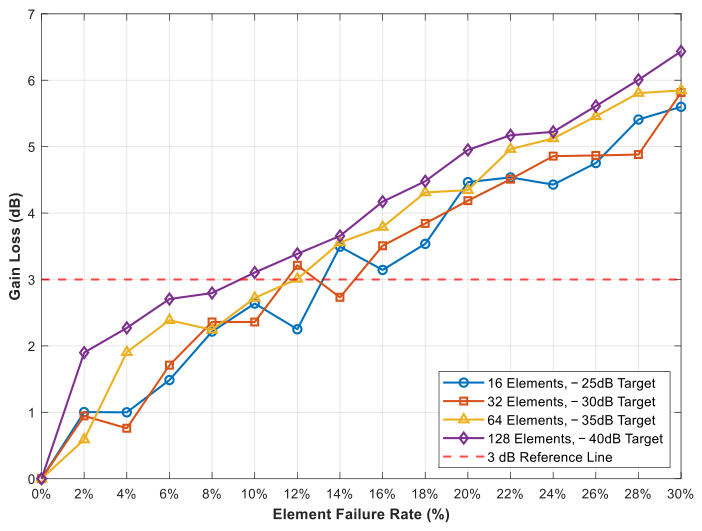
Furthermore, the application of pattern restoration algorithms has clear boundary conditions. There are precedents in related literature using a 30% failure rate as an index for analysis [21]. To find a more accurate range, we conducted simulations on arrays of various scales. As shown in Figure 10, when the failure rate is around 10%, the repaired gain loss already reaches 3 dB; when the failure rate reaches 30%, the gain loss is as high as about 6 dB, and the restoration effect can no longer meet engineering requirements. Based on this, this paper selects a failure rate of 10% to 30% as the index for experimentation.

5. Simulation Results

5.1. Antenna Array Element Failure Diagnosis

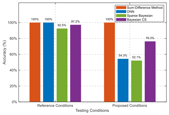
Figure 11 presents a comparison of diagnostic accuracy between the proposed sum-difference method and three alternative algorithms across their respective testing conditions under a 32-element array configuration. Under the reference conditions shown on the left, the proposed method achieves 100% accuracy, demonstrating its exceptional performance even in alternative baseline settings. Under the proposed conditions, which incorporate symmetrical element failures (right side), the accuracy of both the DNN and Sparse Bayesian algorithms drops sharply to approximately 50%, indicating that these methods revert to random guessing and fail to provide effective diagnosis. Although the Bayesian compressive sensing algorithm also integrates phase data, it is inherently limited to sparse scenarios; when the failure rate reaches 20%, its accuracy experiences a substantial decline, despite retaining a modest capability for detecting symmetric failures. Consequently, these results highlight the clear advantages of the proposed method in diagnosing symmetric element faults [22].
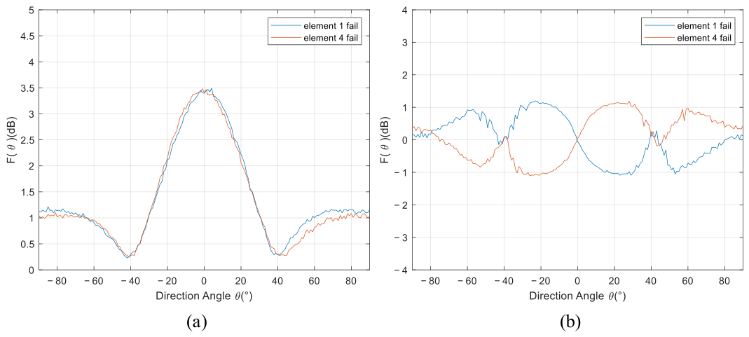
As illustrated in Figure 12, for a four-element linear array experiencing symmetrical failures of elements 1 and 4, the magnitude signatures are nearly identical. However, the corresponding phase patterns exhibit diametrically opposite characteristics. This distinct disparity in the phase domain enables the network to effectively differentiate between the two scenarios, thereby resolving the inherent challenge of diagnosing symmetrical element failures.
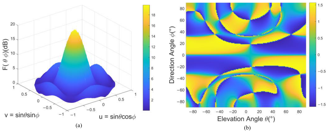
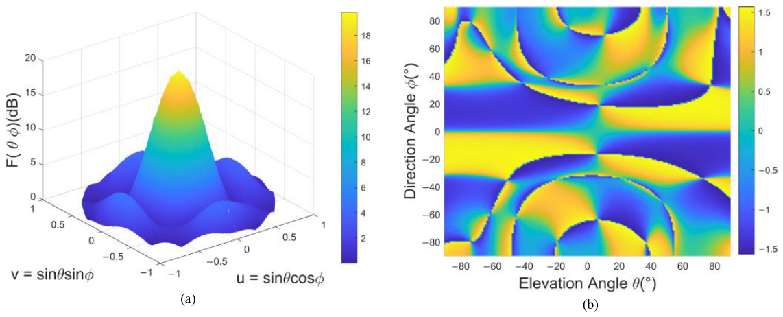
A comparison of Figure 13 and Figure 14 reveals that for the 4 × 4 planar array, the results are consistent with those observed in the linear array. Specifically, the magnitude patterns for element ( 1,1 ) and ( 4,4 ) failures are virtually identical (left figure), whereas their corresponding phase responses are distinctly opposite (right figure).
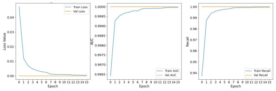
As illustrated in Figure 15, the training and validation performance metrics using the traditional BCE loss function across 15 epochs demonstrate favorable convergence behavior. Specifically, the training loss exhibits a sharp and steady decline from an initial value above 0.045, dropping rapidly within the first few epochs and stabilizing near zero around epoch 8, while the validation loss remains consistently flat and close to zero throughout the entire training process. Concurrently, both the training and validation AUC metrics display exceptionally high performance, starting above 0.996 and rapidly converging toward 1.0 to indicate strong discriminative power across epochs. Furthermore, the training recall increases steeply from approximately 0.937 in the initial epoch and approaches 1.0 by epoch 8, whereas the validation recall stays consistently at the maximum value of 1.0 across all epochs, reflecting a robust capability in identifying positive fault instances.
To evaluate the necessity of the sum-and-difference preprocessing scheme, a comprehensive ablation analysis is conducted across both sample-level diagnostic instances and full-dataset statistical metrics, as detailed in Table 2 and Table 3. Specifically, while the evaluation is performed on the entire test set, 10 representative test samples are randomly selected and presented in Table 2 for intuitive comparison. The results show that while the preprocessed model accurately predicts the ground-truth failure positions, the un-preprocessed model yields erratic predictions laden with severe misjudgments. This occurs because, without preprocessing, the data corresponding to symmetrical element failures exhibit extreme similarity; to the neural network, this manifests as a single data pattern associated with multiple conflicting labels. Consequently, the network fails to distinguish them and resorts to random guessing, which is directly evidenced by the near-50% performance metrics of the un-preprocessed dataset in Table 3, and in severe cases—such as sample 9 in Table 2—this causes the model to erroneously label multiple or incorrect positions as failures. Expanding this evaluation to the full test set, Table 3 quantitatively demonstrates the distinct performance discrepancy, where the un-preprocessed model achieves a macro-averaged precision of 57.04%, a recall of 57.8%, an F1-score of 57.42%, and an exact-match accuracy of only 17.43%, whereas the preprocessed model attains 100% across all evaluated metrics. This comprehensive contrast confirms that the proposed preprocessing mechanism is vital for eliminating structural ambiguity and ensuring robust diagnostic reliability across the entire dataset.

5.2. Pattern Recovery

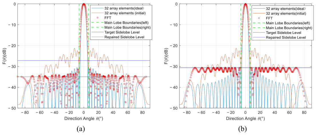
When the target sidelobe level is within the achievable range of the array, the restoration results with and without the adaptive threshold are identical, and both can successfully achieve the target value. However, when the target sidelobe value represents an unattainable standard, the adaptive threshold FFT method exhibits a substantial advantage. As illustrated in Figure 16, a 32-element array with faulty elements at positions 7 and 8 is considered. Figure 16a shows the restoration result without applying the adaptive threshold. The initial target is set to −35 dB, which is an unachievable goal under the given array conditions. Consequently, the restored peak sidelobe level (PSLL) only reaches −27.19 dB; this is visually represented by a significant deviation between the black and blue lines, falling far short of the requirement. In contrast, Figure 16b demonstrates the recovery result utilizing the proposed adaptive threshold. Through dynamic adjustment, the restored PSLL is successfully improved to −30.63 dB, evidenced in the figure by the nearly perfect overlap of the black and blue lines.
As presented in Table 4 and Table 5, a statistical performance evaluation is conducted across different array scales (16, 32, and 64 elements with corresponding target sidelobe levels of −25 dB, −30 dB, and −35 dB) and various failure rates (5%, 10%, and 15%) to validate the effectiveness of the adaptive algorithm compared to the non-adaptive counterpart. Across all tested scenarios, both algorithms maintain a 0% convergence failure rate, demonstrating robust convergence stability under diverse fault topologies. Furthermore, the statistical results show that the adaptive algorithm consistently reduces the average iteration times across all configurations, achieving an overall average optimization of approximately 21%. Specifically, the iteration count optimization ranges from 4% to 30%, with certain cases even exceeding 30% (such as a 33.16% reduction for the 16-element array at a 5% failure rate). The comprehensive statistical distribution of standard deviation, convergence failure rate, and average iteration times confirms that our algorithm achieves better performance stability. In addition, the execution time for all experiments using the adaptive-threshold-based FFT algorithm in the table is within 2 s.
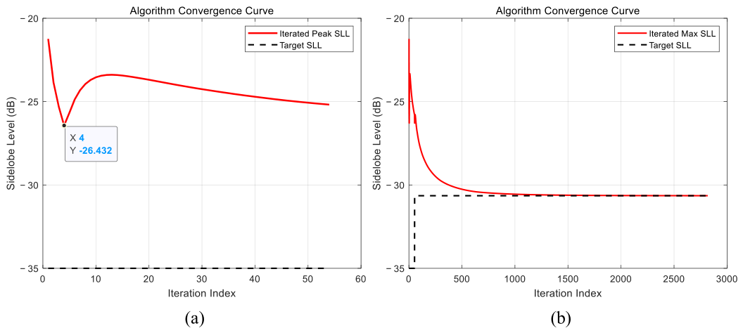
Figure 17 presents the results obtained under a 32-element array configuration with elements 7 and 8 failing, and a target sidelobe level of −35 dB. The left panel shows the iteration curve of the fixed-threshold algorithm; although it converges quickly, the optimal result deviates significantly from the target value. The right panel displays the iteration curve of the adaptive-threshold algorithm, where the repair performance is noticeably superior. Although it requires a higher number of iterations, this is an acceptable trade-off.
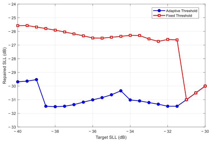
Figure 18 shows the final PSLL of the two algorithms under different initial thresholds for a 32-element array with failures at the 7th and 8th elements. It can be seen that the adaptive threshold algorithm exhibits a distinct advantage below −31 dB.
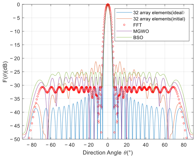
Figure 19 presents a comparison of the final restoration results achieved by different algorithms. Here, the circles represent the proposed algorithm, the purple line denotes the multi-strategy Grey Wolf Optimizer (MGWO), and the green line indicates the Brain Storm Optimization (BSO). A comparative analysis reveals that the restoration performance of the proposed algorithm is significantly superior to that of the other two. In terms of computational efficiency under identical conditions, MGWO requires approximately 40 s and BSO takes about 30 s, whereas the proposed algorithm completes the process in less than 1 s, demonstrating a massive advantage in time cost. Furthermore, heuristic optimization algorithms inherently exhibit randomness in their restoration results, but the proposed method completely avoids this issue, yielding stable and deterministic outcomes.
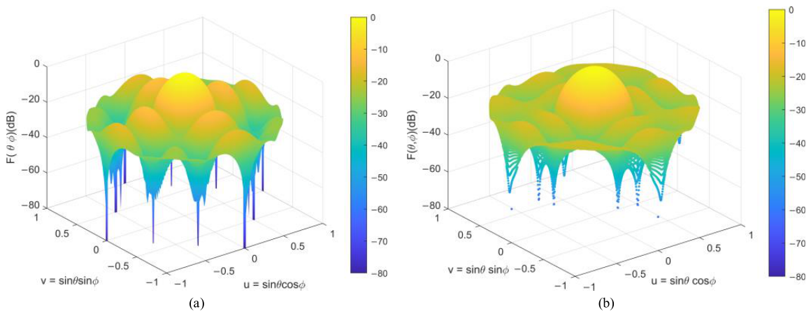
Figure 20 illustrates the recovery performance for a 2D array. For a 6 × 6 planar array with element failures at ( 1,1 ) and ( 4,4 ) , the left figure exhibits an unrecovered pattern with a PSLL of −11.83 dB. Conversely, the right figure demonstrates the recovered pattern using the proposed algorithm, where the PSLL drops to −17.78 dB, yielding an optimization improvement of 5.95 dB.

5.3. Systematic Performance Analysis

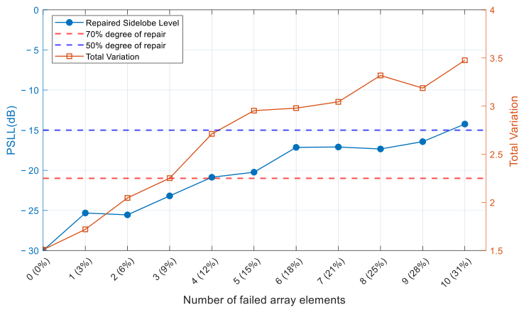
The following experiments are all based on a 32-element linear array. Figure 21 quantitatively demonstrates the synchronous evolution of the progressive degradation in recovery performance and the severe oscillation of excitation weights under varying fault ratios. As observed from the blue curve representing the repaired PSLL, as the number of failed elements increases from 0 to 10 (a fault ratio of 31%), the array’s PSLL exhibits a gradual, step-like degradation from the initial −30 dB, indicating a progressive performance deterioration rather than a sudden algorithmic collapse. Specifically, when the fault ratio reaches 12% (4 failed elements), the recovery performance drops to the 70% baseline; as the fault ratio approaches 31%, the PSLL further degrades to the 50% baseline around −15 dB, signifying a severe and irreversible distortion in the array’s radiation pattern. Concurrently, the orange curve, representing the total variation in adjacent element amplitudes, precisely characterizes the physical critical point of degree-of-freedom exhaustion. When the fault ratio is below 9% (up to 3 failed elements), the total variation increases slowly, indicating that the system possesses sufficient degrees of freedom and the energy redistribution executed by the algorithm is smooth and physically realizable. However, as the fault ratio enters the critical range of 9% to 15% (3 to 5 failed elements), the total variation curve exhibits a steep upward trend. This sharp increase mathematically demonstrates that, in order to forcibly maintain the sidelobe suppression, the algorithm begins to assign extremely unbalanced and conflicting excitation weights to the remaining healthy elements. Such violent oscillation in weights directly signifies the exhaustion of the array’s available degrees of freedom, leading to a drastic decline in the algorithm’s control over the far-field radiation pattern.
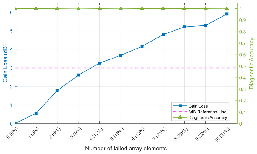
Figure 22 quantitatively illustrates the evolutionary relationship between the gain loss and the diagnostic accuracy under varying fault ratios. As observed from the green curve representing diagnostic accuracy, the diagnostic module exhibits exceptional robustness, consistently maintaining a perfect 100% accuracy across the entire testing range from 0 to 10 failed elements (a fault ratio of 0% to 31%), remaining completely unaffected by the expanding scale of the faults. However, despite the flawless performance of the front-end diagnosis, the blue curve representing gain loss exhibits a significant and monotonic upward trend. As the number of damaged elements increases, the system pays a heavy penalty in energy redistribution to forcibly suppress the sidelobes. Notably, the pink dashed line represents the 3 dB reference line, which signifies a 50% loss of the main lobe radiation power in practical engineering. The gain loss curve crosses this critical threshold between 3 (9%) and 4 (12%) failed elements, indicating that the array has lost half of its radiated energy at this point. When the fault ratio reaches 31%, the gain loss severely approaches 6 dB. These results rigorously demonstrate that while the diagnostic algorithm possesses perfect stability, the practical engineering value of the array degrades substantially once the fault ratio exceeds the 9–12% range due to the inherent loss of physical aperture and the compensation cost.
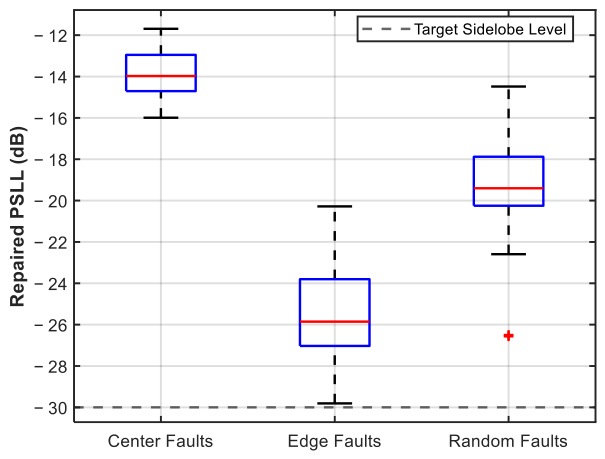
Figure 23 quantitatively illustrates the performance sensitivity of the proposed algorithm to distinct fault locations on a 32-element linear array under a fixed failure scale of four damaged elements. In the boxplot, the central red horizontal line inside each blue box represents the statistical median of the repaired PSLL for each respective fault group, while the upper and lower boundaries of the blue box indicate the 25th and 75th percentiles, defining the interquartile range of the normal data spread. The black dashed whiskers extending vertically from the boxes denote the overall range of typical data variation, and the red cross symbol (+) appearing in the random faults group represents a statistical outlier that exceeds the regular distribution limits. As revealed by these statistical indicators, edge faults exhibit the most favorable sidelobe suppression performance with a median dropping to approximately −25 dB, whereas center faults present the greatest challenge with an elevated median around −14.3 dB, while random faults yield a moderate median of roughly −19.3 dB alongside localized performance fluctuations. These statistical results indicate that failures occurring in different spatial regions alter the utilization efficiency of the available degrees of freedom, thereby demonstrating the inherent spatial sensitivity of the array restoration process.

6. Conclusions

Regarding the detection of faulty elements in array antennas, in this paper, we propose a deep learning method based on sum-and-difference beams. The proposed method utilizes processed far-field amplitude and phase data as the network input to output the indices of the faulty elements. This approach effectively resolves the inherent difficulty in identifying symmetric element faults and achieves exceptionally high accuracy, thereby providing a novel pathway for real-time array diagnosis in complex environments. Furthermore, to address the performance recovery of degraded radiation patterns, we introduce an iterative FFT method based on an adaptive threshold. This method is capable of selecting the most appropriate value between the target SLL and the theoretical optimal SLL for the iterative process. Concurrently, by employing sidelobe suppression with an adaptive step size, the algorithm successfully reduces the required number of iterations, leading to a further enhancement in overall algorithmic performance.
Although in this study we establish the theoretical framework and validate the proposed method through extensive simulations, due to the complexity of hardware implementation, physical experimental validation using a hardware prototype is currently lacking. Therefore, implementing this algorithm on a real-world array platform and conducting anechoic chamber measurements will be a primary focus of our future work. Concurrently, we will also expand our investigation to address complex physical factors and broader extreme failure scenarios.
It should be explicitly noted that while robust diagnostic and restorative performance—with diagnostic accuracy approaching 100%—is achieved at scales like 4 × 4, 6 × 6, and 8 × 8, the cross-scale adaptability of the proposed algorithm remains theoretically constrained. Fundamentally, the fixed-dimension input and output constraints of the CNN mathematically limit the algorithm’s direct application to arbitrary, higher-dimensional ultra-large-scale arrays. Expanding the network to accommodate massive array structures currently poses significant challenges due to hardware limitations and data generation constraints. While existing literature has proposed array zero-padding techniques and subarray partitioning structures as potential solutions for scale transitions [23,24], directly applying these engineering strategies introduces complex boundary coupling effects and alters the effective aperture resolution during iterations, which remain theoretically unverified in our current framework. Therefore, extending this methodology to achieve strict cross-scale diagnosis without performance degradation remains an important theoretical defect of the current model. In future work, we will focus on rigorously exploring and mathematically verifying subarray topological structures and dynamic zero-padding compensation mechanisms to fundamentally resolve the dimensional constraints of deep learning-based array diagnosis.

Author Contributions

Conceptualization, X.G. and S.D.; methodology, H.Z., S.D. and Z.Z.; validation, W.Z. and S.D.; investigation, W.Z. and J.Z.; writing—review and editing, X.G. and S.D.; supervision, S.D. and J.Z. All authors have read and agreed to the published version of the manuscript.

Funding

This research received no external funding.

Data Availability Statement

The original contributions presented in this study are included in the article. Further inquiries can be directed to the corresponding author.

Conflicts of Interest

Author Sheng Ding was employed by the company Zhejiang Geespace Technology Co., Ltd. The remaining authors declare that the research was conducted in the absence of any commercial or financial relationships that could be construed as a potential conflict of interest.

References

  1. Cheng, Y.-F.; Ding, X.; Shao, W.; Liao, C. A High-Gain Sparse Phased Array with Wide-Angle Scanning Performance and Low Sidelobe Levels. IEEE Access 2019, 7, 31151–31158. [Google Scholar] [CrossRef] [Scilit]
  2. Keizer, W.P.M.N. Element Failure Correction for a Large Monopulse Phased Array Antenna with Active Amplitude Weighting. IEEE Trans. Antennas Propag. 2007, 55, 2211–2218. [Google Scholar] [CrossRef] [Scilit]
  3. Moretta, R.; Leone, G.; Maisto, M.A.; Pierri, R.; Solimene, R. Array Faulty Element Diagnostics by Few Phaseless Data and Convex Optimization. In Proceedings of the 2023 17th European Conference on Antennas and Propagation (EuCAP), Florence, Italy, 26–31 March 2023; pp. 1–4. [Google Scholar] [CrossRef] [Scilit]
  4. Dell’Aversano, A.; Natale, A.; Cuccaro, A.; Solimene, R. Linear Array Antenna Diagnostics Through a MUSIC Algorithm. IEEE Access 2019, 7, 176952–176959. [Google Scholar] [CrossRef] [Scilit]
  5. Cui, W.; Li, L.; Li, H.; Guan, F.; Hong, D.; Liu, G. Dependency Matrix-Based Fast Fault Diagnosis Using Search Algorithm. IEEE Trans. Instrum. Meas. 2023, 72, 3510908. [Google Scholar] [CrossRef] [Scilit]
  6. Yao, H.M.; Li, M.; Jiang, L.; Yeung, K.L.; Ng, M. Antenna Array Diagnosis Using a Deep Learning Approach. IEEE Trans. Antennas Propag. 2024, 72, 5396–5401. [Google Scholar] [CrossRef] [Scilit]
  7. Chen, K.; Wang, W.; Chen, X.; Yin, H. Deep Learning Based Antenna Array Fault Detection. In Proceedings of the 2019 IEEE 89th Vehicular Technology Conference (VTC2019-Spring), Kuala Lumpur, Malaysia, 28 April–1 May 2019; pp. 1–5. [Google Scholar] [CrossRef] [Scilit]
  8. Vaquero, Á.F.; Córcoles, J. Convex Formulations for Antenna Array Pattern Optimization Through Linear, Quadratic, and Second-Order Cone Programming. Mathematics 2025, 13, 1796. [Google Scholar] [CrossRef] [Scilit]
  9. Jiang, X.; Qin, J.; Jiang, T. Comparing the Failure Correction Ability between GA and FA for Array Antenna. In Proceedings of the 2019 Joint International Symposium on Electromagnetic Compatibility, Sapporo and Asia-Pacific International Symposium on Electromagnetic Compatibility (EMC Sapporo/APEMC), Sapporo, Japan, 3–7 June 2019; pp. 737–740. [Google Scholar] [CrossRef] [Scilit]
  10. Kala, D.D.; Sundari, D. A review on optimization of antenna array by evolutionary optimization techniques. Int. J. Intell. Unmanned Syst. 2021, ahead-of-print. [Google Scholar] [CrossRef] [Scilit]
  11. Zhang, X.; Li, Y.; Yang, X.; Zheng, L.; Long, T.; Baker, C.J. A Novel Monopulse Technique for Adaptive Phased Array Radar. Sensors 2017, 17, 116. [Google Scholar] [CrossRef] [Scilit] [PubMed]
  12. Zhao, W.; Zhang, H.; Zou, J.; Liu, G.; Shu, F. Effective Chirp Modulation Communication System Design for LEO Satellite IoT. IEEE Internet Things J. 2025, 12, 16962–16976. [Google Scholar] [CrossRef] [Scilit]
  13. Wang, Z.A.; Phaseless, P.L. Diagnosis and Pattern Correction of Faulty Antenna Arrays via Advanced Bayesian Compressive Sensing Approaches. Electromagn. Sci. 2025, 3, 0090382. [Google Scholar] [CrossRef] [Scilit]
  14. Zhao, W.; Qi, R.; Zou, J.; Liu, G.; Sun, L.; Shu, F. Optimization of Protection Interval for Chirp Modulation in LEO Satellite Communications. IEEE Wirel. Commun. Lett. 2026, 15, 1866–1870. [Google Scholar] [CrossRef] [Scilit]
  15. Li, M.; Franek, O.; Zhang, F.; Wang, Z.; Fan, W. Over-the-Air Testing for Connecting Faults Diagnosis in Beamforming Antenna Arrays With Short Measurement Distance. IEEE Trans. Instrum. Meas. 2023, 72, 8004613. [Google Scholar] [CrossRef] [Scilit]
  16. Jiang, H.; Pan, X.; Shi, W.; Zeng, L.; Chen, Z.; Shu, F.; Wang, J. Deep Reinforcement Learning Enabled UAV Trajectory Optimization for A2G Communication Systems. IEEE Trans. Cogn. Commun. Netw. 2026, 12, 3164–3178. [Google Scholar] [CrossRef] [Scilit]
  17. Peters, T.J. A conjugate gradient-based algorithm to minimize the sidelobe level of planar arrays with element failures. IEEE Trans. Antennas Propag. 1991, 39, 1497–1504. [Google Scholar] [CrossRef] [Scilit]
  18. Jiang, H.; Shi, W.; Chen, X.; Zhu, Q.; Chen, Z. High-Efficient Near-Field Channel Characteristics Analysis for Large-Scale MIMO Communication Systems. IEEE Internet Things J. 2025, 12, 7446–7458. [Google Scholar] [CrossRef] [Scilit]
  19. Chen, Y.-S.; Tsai, I.-L. Detection and Correction of Element Failures Using a Cumulative Sum Scheme for Active Phased Arrays. IEEE Access 2018, 6, 8797–8809. [Google Scholar] [CrossRef] [Scilit]
  20. Zhang, Z.; Wong, K.-K.; Dang, J.; Zhang, Z.; Masouros, C.; Chae, C.-B. On Fundamental Limits of Slow-Fluid Antenna Multiple Access for Unsourced Random Access. IEEE Wirel. Commun. Lett. 2025, 14, 3455–3459. [Google Scholar] [CrossRef] [Scilit]
  21. Zou, S.; Gu, W.; Ren, W.; Shen, C.; Chen, Z.; Hao, L. Functional Damage Assessment Method for Preformed Fragment Warheads to Evaluate the Effect on the Phased-Array Antenna. Electronics 2023, 12, 1907. [Google Scholar] [CrossRef] [Scilit]
  22. Available online: https://github.com/6gxy/Element-Failure-Diagnosis-and-Pattern-Recovery-for-Array-Antennas (accessed on 2 August 2026).
  23. Mailloux, R. Phased Array Antenna Handbook, 3rd ed.; Artech: Thiruvananthapuram, India, 2017. [Google Scholar]
  24. Hong, W.; Jiang, Z.H.; Yu, C.; Zhou, J.; Chen, P.; Yu, Z.; Zhang, H.; Yang, B.; Pang, X.; Jiang, M.; et al. Multibeam Antenna Technologies for 5G Wireless Communications. IEEE Trans. Antennas Propag. 2017, 65, 6231–6249. [Google Scholar] [CrossRef] [Scilit]
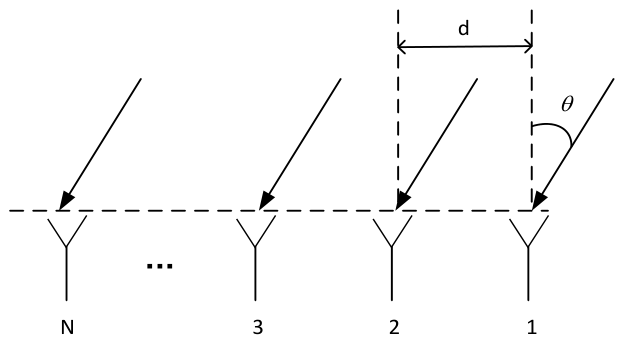
Figure 1. Schematic of a one-dimensional uniform linear array.
Electronics 15 03717 g001
Figure 2. Schematic of a two-dimensional planar array.
Electronics 15 03717 g002
Figure 3. Comparison between ideal radiation pattern and failure radiation pattern: (a) Element failures at different locations. (b) Element failures with varying numbers.
Electronics 15 03717 g003
Figure 4. Schematic diagrams of various faulty element positions in an 8-element linear array: (a) Element 1 failure (red part). (b) Element 5 failure (red part).
Electronics 15 03717 g004
Figure 5. Schematic diagrams of varying numbers of faulty elements in an 8-element linear array: (a) One-element failure (red part). (b) Two-element failure (red part). (c) Three-element failure (red part).
Electronics 15 03717 g005
Figure 6. Four-element linear array.
Electronics 15 03717 g006
Figure 7. The architecture of the proposed CNN model.
Electronics 15 03717 g007
Figure 8. Radiation pattern synthesis using the FFT method.
Electronics 15 03717 g008
Figure 9. FFT-based pattern recovery with adaptive step size and thresholding.
Electronics 15 03717 g009
Figure 10. Gain loss versus element failure rate under different array sizes and target sidelobe levels.
Electronics 15 03717 g010
Figure 11. Accuracy comparison between the proposed algorithm and other algorithms under their respective conditions.
Electronics 15 03717 g011
Figure 12. Test performance on a four-element linear array. (a) Magnitude response. (b) Phase response.
Electronics 15 03717 g012
Figure 13. Element (1, 1) failure in a 4 × 4 array. (a) Magnitude response. (b) Phase response.
Electronics 15 03717 g013
Figure 14. Element (4, 4) failure in a 4 × 4 array. (a) Magnitude response. (b) Phase response.
Electronics 15 03717 g014
Figure 15. BCE loss training log.
Electronics 15 03717 g015
Figure 16. Comparison of recovery results under an unachievable target sidelobe level. (a) Result without adaptive thresholding. (b) Result with adaptive thresholding.
Electronics 15 03717 g016
Figure 17. Comparison of iteration curves: (a) Iteration curves based on the fixed-threshold algorithm. (b) Iteration curves based on the adaptive-threshold algorithm.
Electronics 15 03717 g017
Figure 18. Final PSLL under different initial thresholds.
Electronics 15 03717 g018
Figure 19. Performance comparison of different restoration algorithms.
Electronics 15 03717 g019
Figure 20. Algorithm recovery results for the 6 × 6 array. (a) Faulty radiation pattern. (b) Recovered radiation pattern.
Electronics 15 03717 g020
Figure 21. PSLL recovery performance and total variation in excitation weights versus the number of failed elements.
Electronics 15 03717 g021
Figure 22. Gain loss and diagnostic accuracy versus the number of failed array elements.
Electronics 15 03717 g022
Figure 23. Statistical distribution of repaired PSLL under different fault locations (red line: median; blue box: 25th–75th percentiles; whiskers: range; ‘+’: outlier; black dashed line: target SLL).
Electronics 15 03717 g023
Table 1. Network specifications.
TypeFilter/NeuronFilter SizeInput SizeOutput Size
Convolution1
ReLU
323 × 323 × 4623 × 46 × 32
Convolution2
ReLU
643 × 323 × 46 × 3211 × 23 × 64
Convolution3
ReLU
1283 × 311 × 23 × 645 × 11 × 128
Fully Connected Layer1
ReLU
256 5 × 11 × 128256
Fully Connected Layer2
ReLU
128 256128
Output
Sigmoid
12816
Table 2. Diagnostic results.
Sample NumberSample IndexFailure PositionPreprocessedUn-Preprocessed
162148 14 158 14 153 8 9 15
227188 11 138 11 136 8 9 13
360294 9 144 9 149 13 14
4267992 10 122 10 1210 12 15
581354 12 144 12 143 12 13
611975 8 135 8 139 12 13
7295752 8 132 8 132 4 9
8228556 9 126 9 126 9 12
9967 127 125 7 10 12
10235496 8 166 8 166 8 16
Table 3. Diagnostic indicators.
Dataset TypeMacro-Averaged PrecisionRecallF1-ScoreExact-Match Accuracy
Un-Preprocessed57.04%57.8%57.42%17.43%
Preprocessed100%100%100%100%
Table 4. Performance indicators without adaptive algorithms.
Sample TypeFailure RateStandard DeviationConvergence Failure RateAverage Iteration Times
5%794.440%803.3
16(−25 dB)10%185.860%143.4
15%6016.260%1989.9
5%717.470%403.3
32(−30 dB)10%195.510%117.7
15%14.780%60.3
5%707.080%279.8
64(−35 dB)10%18.410%63.5
15%4.50%54.6
Table 5. Performance indicators of adaptive algorithms.
Sample TypeFailure RateStandard DeviationConvergence Failure RateAverage Iteration TimesOptimization Degree of Iteration Times
5%517.760%536.933.16%
16 (25 dB)10%116.590%108.824.13%
15%4012.410%1343.532.48%
5%473.270%276.231.52%
32(−30 dB)10%124.570%92.521.41%
15%7.410%55.38.29%
5%481.650%204.227.02%
64(−35 dB)10%8.110%56.511.02%
15%1.770%52.34.21%
Disclaimer/Publisher’s Note: The statements, opinions and data contained in all publications are solely those of the individual author(s) and contributor(s) and not of MDPI and/or the editor(s). MDPI and/or the editor(s) disclaim responsibility for any injury to people or property resulting from any ideas, methods, instructions or products referred to in the content.