A Real-Time Communication Framework for Distributed Wearable Human Activity Recognition

Abstract

Real-time multi-sensor human activity recognition (HAR) requires accurate models and a system architecture capable of distributing computation, exchanging compact outputs, and maintaining temporal consistency across asynchronous streams. This paper presents a distributed HAR framework in which five wearable sensors are associated with local embedded nodes that perform acquisition, windowing, preprocessing, and convolutional neural network–long short-term memory (CNN–LSTM) inference. Each node transmits a timestamped six-class softmax vector, and a central node applies approximate synchronization and learned probability-level fusion. The framework was evaluated with ten participants whose data were not used for model development. It achieved 95.868% accuracy and a 95.642% macro-F1-score. During continuous operation, the system sustained 47.949 predictions/s, with a mean post-window end-to-end latency of 33.963 ms and a mean synchronization span of 13.788 ms. Relative to complete-window transmission, the numerical payload decreased by 97.69%, and central-node energy per prediction decreased by 52.2% compared with centralized real-time processing. Under 30% independent probability-message loss, accuracy remained at 94.31%.

1. Introduction

Sensor-based Human Activity Recognition (HAR) has evolved from an algorithmic classification problem into a real-time embedded sensing challenge. Public inertial datasets have demonstrated that wearable and smartphone signals can support accurate recognition of daily activities [1,2]. Concurrently, convolutional neural networks (CNNs), recurrent networks, and hybrid CNN–long short-term memory (CNN–LSTM) architectures have improved the representation of spatial and temporal motion patterns [3,4,5,6,7], while ensemble learning, hybrid models, domain adaptation, smartphone-based methods, and real-time deep architectures have further advanced classification performance [8,9,10,11,12,13]. However, deploying multi-sensor HAR requires more than selecting an accurate model. A practical system must determine where inference is executed, which information is transmitted, how predictions from different body locations are temporally aligned, and whether the complete pipeline satisfies runtime and energy constraints.

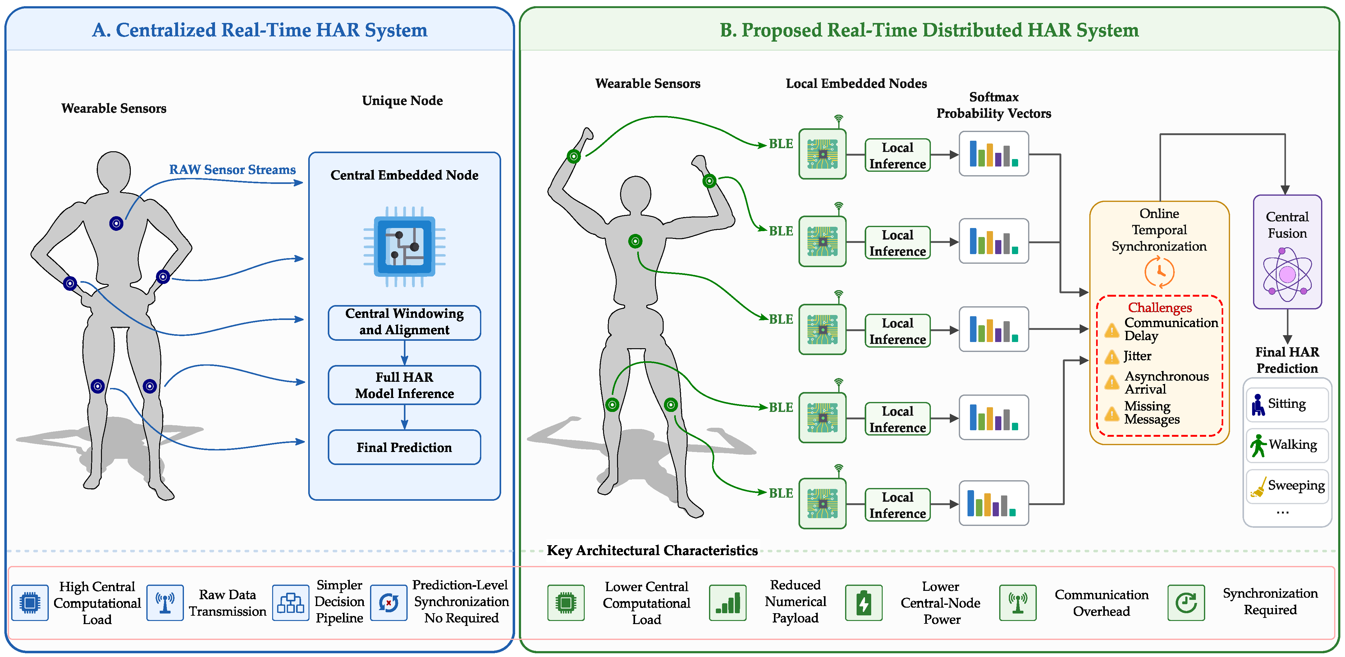
A centralized real-time architecture collects the sensor measurements at a single processing node and executes the complete inference pipeline there. This simplifies prediction-level coordination but concentrates data handling, window construction, preprocessing, model inference, and energy demand at the central device. A distributed architecture instead assigns sensor-specific inference to local embedded nodes and transmits compact model outputs for central fusion. This reduces the raw-data processing assigned to the central node but introduces communication delay, jitter, asynchronous arrival, missing messages, and temporal synchronization as factors that can directly affect the fusion input.

Figure 1 illustrates this architectural trade-off. Both alternatives use the same physical wearable sensing configuration and operate in real time; the primary distinction is the location of neural processing and the representation transmitted to the central node.

The architectural implications illustrated in Figure 1 are summarized in

Table 1. Architectural trade-offs between centralized and distributed real-time HAR inference.

Aspect	Centralized Real-Time HAR	Distributed Real-Time HAR
Processing placement	Central node	Local nodes and central fusion
Transmitted representation	Raw sensor measurements	Local probability vectors
Central computational load	High	Lower
Prediction-level synchronization	Not required	Required
Primary system challenge	Central computation and raw data handling	Communication, synchronization, and fallback operation

.

1.1. Related Work and Research Gap

Multi-sensor HAR combines complementary information from different anatomical locations and can distinguish activities that may not be adequately represented by a single wearable sensor [14,15]. Nevertheless, increasing the number of sensing locations also introduces practical challenges involving sensor selection, communication, temporal alignment, and deployment complexity [16,17]. Edge computing addresses part of this problem by placing processing closer to the data source [18,19]. Lightweight deep models, binarized networks, optimized DeepConvLSTM architectures, and wearable-device implementations have demonstrated that HAR inference can be executed on resource-constrained hardware [20,21,22,23,24]. These studies primarily establish the feasibility of embedded or device-level inference, where classification accuracy must be balanced against latency, memory, communication, and power consumption [25,26].

Real-time HAR also requires evaluation beyond model-centered classification metrics. End-to-end latency, inference time, communication delay, and temporal consistency determine whether predictions remain useful during continuous operation [12,27,28]. Energy-aware sensing, efficient neural architectures, and embedded accelerators have consequently been investigated to support sustained wearable inference [29,30]. However, many edge artificial intelligence (Edge AI) studies focus on optimizing inference on an individual device or central edge processor rather than coordinating simultaneous predictions generated by multiple wearable nodes.

Distributed and federated HAR methods provide additional mechanisms for decentralizing computation or data use [31,32]. Approaches such as Meta-HAR and graph–temporal models address personalization, distributed learning, or relationships among sensors and users [33,34]. Federated HAR, however, primarily distributes model training or adaptation while retaining local data; it does not inherently address online inference in which several embedded nodes simultaneously generate outputs that must be communicated, temporally aligned, and fused during live operation. Real-time distributed sensing has also been investigated in applications such as human–robot collaboration [35], but the combined behavior of probability-level communication, timestamp-based synchronization, fallback operation, and neural fusion across multiple body-worn devices remains insufficiently evaluated.

Accordingly, the novelty of this study is not a new CNN–LSTM classifier or the use of edge hardware alone. Unlike Edge AI approaches centered on efficient inference within an individual device, federated approaches centered on distributed training, and distributed sensing studies without explicit prediction-level synchronization, this work investigates the complete operation of a multi-node wearable HAR inference pipeline. Local neural inference, timestamped probability communication, online synchronization, fallback behavior, central fusion, and system-level measurements are integrated and evaluated within the same real-time implementation.

Table 2. Contextual comparison with representative real-time and decentralized HAR systems.

Study	Processing Organization	Communication and Synchronization	Reported System-Level Results
Alexan et al. [23]	Wrist-sensor data processed through a local or cloud application programming interface (API)	Raw accelerometer and gyroscope data; no multi-node prediction synchronization	94.89% accuracy; latency, traffic, and energy not reported
WatchHAR [24]	Audio and inertial inference executed entirely on a smartwatch	No inter-node communication or fusion synchronization	More than 90% accuracy and 11.8 ms multimodal classification time; energy not reported
Shi et al. [28]	Capsule-based recognition with Long-Range (LoRa) sensor communication	Wireless sensor-data transmission; prediction-level multi-node synchronization not evaluated	Real-time operation reported; directly comparable latency, traffic, and energy values not reported
Meta-HAR [33] and EGTCN [34]	Federated model training and personalized or local inference	Model updates are exchanged during training rather than simultaneous local predictions during inference	Dataset-dependent classification results; live synchronization, inference traffic, and runtime energy not evaluated
Belcamino et al. [35]	Distributed multimodal recognition for human–robot collaboration	Inertial measurement unit (IMU) and visual–tactile modalities fused for application-specific real-time recognition	Offline and real-time recognition evaluated; probability-stream synchronization, traffic, and energy not reported
Proposed framework	Five local CNN–LSTM models and central probability-level fusion	Timestamped probability messages, approximate time synchronizer (ATS), and fallback operation	95.868% accuracy, 95.642% macro-F1, 33.963 ms post-window latency, and central-node energy and communication analysis

positions the proposed framework relative to representative real-time, edge-based, federated, and distributed HAR systems. Because these studies use different datasets, activities, hardware platforms, and timing definitions, their reported values provide contextual evidence rather than a controlled performance ranking. The comparison therefore emphasizes differences in processing organization, communication strategy, synchronization support, and system-level evaluation scope.

The representative systems in Table 2 address complementary aspects of practical HAR, including cloud-based recognition, fully on-device execution, long-range sensor communication, federated training, and multimodal human–robot interaction. However, they do not jointly evaluate timestamped probability-level communication, prediction-level synchronization across multiple body-worn inference nodes, controlled message unavailability, and central-node energy consumption. The proposed framework addresses this combined systems-level problem and includes a centralized real-time reference using the same five sensors.

1.2. Proposed Framework and Contributions

The proposed framework uses five wearable inertial sensors associated with local embedded nodes. Each node acquires its assigned sensor stream, constructs temporal windows, applies the preprocessing used during training, and executes a sensor-specific CNN–LSTM model. Rather than transmitting complete raw-signal windows, the local nodes communicate timestamped six-class probability vectors. The central node temporally aligns the received vectors, constructs the fusion input, and generates the global activity prediction.

The sensing configuration and trained models are based on the multi-sensor dataset reported in [2] and the distributed HAR architecture introduced in [36]. The present work does not seek to revalidate that offline model architecture. Instead, it extends it into a physically distributed real-time system and evaluates the consequences of local inference, network communication, temporal synchronization, and central fusion under live and controlled adverse conditions. The robot operating system (ROS) was used as the implementation middleware for message exchange, coordination, and logging, but the architectural principles are applicable to other platforms supporting timestamped communication and temporal alignment.

The main contributions are:

• Real-Time Distributed Wearable Inference: An implemented multi-node HAR architecture in which five local embedded devices perform sensor-specific CNN–LSTM inference and contribute to a central decision during continuous operation.
• Timestamped Probability-Level Communication: A message representation that transmits compact local softmax vectors and timing metadata instead of complete raw-signal windows, enabling communication-payload quantification, source traceability, and temporal fusion.
• Synchronization and Fallback Operation: An online mechanism that aligns independently generated local predictions and maintains global inference during temporary synchronization or message-availability failures.
• System-Level and Comparative Evaluation: An experimental assessment covering classification performance, participant variability, latency, throughput, synchronization, communication payload, robustness under message loss and node disconnection, and central-node energy consumption. A centralized real-time reference is also evaluated using the same five physical sensor locations to quantify the implications of changing the processing architecture.

The remainder of this paper is organized as follows: Section 2 describes the sensing setup, embedded hardware, neural network models, experimental protocol, robustness scenarios, and evaluation metrics. Section 3 presents the distributed inference architecture, communication protocol, synchronization and fallback mechanisms, central fusion, and runtime instrumentation. Section 4 reports the classification, latency, throughput, synchronization, communication, robustness, and energy results, including the centralized real-time comparison. Section 5 discusses the implications, limitations, and future extensions of the framework, and Section 6 presents the conclusions.

2. Materials and Methods

This section describes the sensing configuration, embedded hardware, neural network models, experimental protocol, robustness scenarios, and evaluation metrics used to assess the proposed real-time distributed HAR framework. The wearable configuration follows the multi-sensor setup introduced in previous work [36], while the present study focuses on its physically distributed deployment, probability-level communication, temporal synchronization, and runtime operation.

2.1. Materials and Experimental Setup

The experimental platform comprised five MetaMotionRL wearable sensors (version r0.5) from MbientLab Inc. (San Jose, CA, USA); three NVIDIA Jetson Nano and two Jetson Orin Nano devices from NVIDIA Corporation (Santa Clara, CA, USA) as local inference nodes; a Jetson AGX Xavier as the central processing node; and a dedicated wireless network implemented using a Dream Router 7 from Ubiquiti Inc. (San Jose, CA, USA).

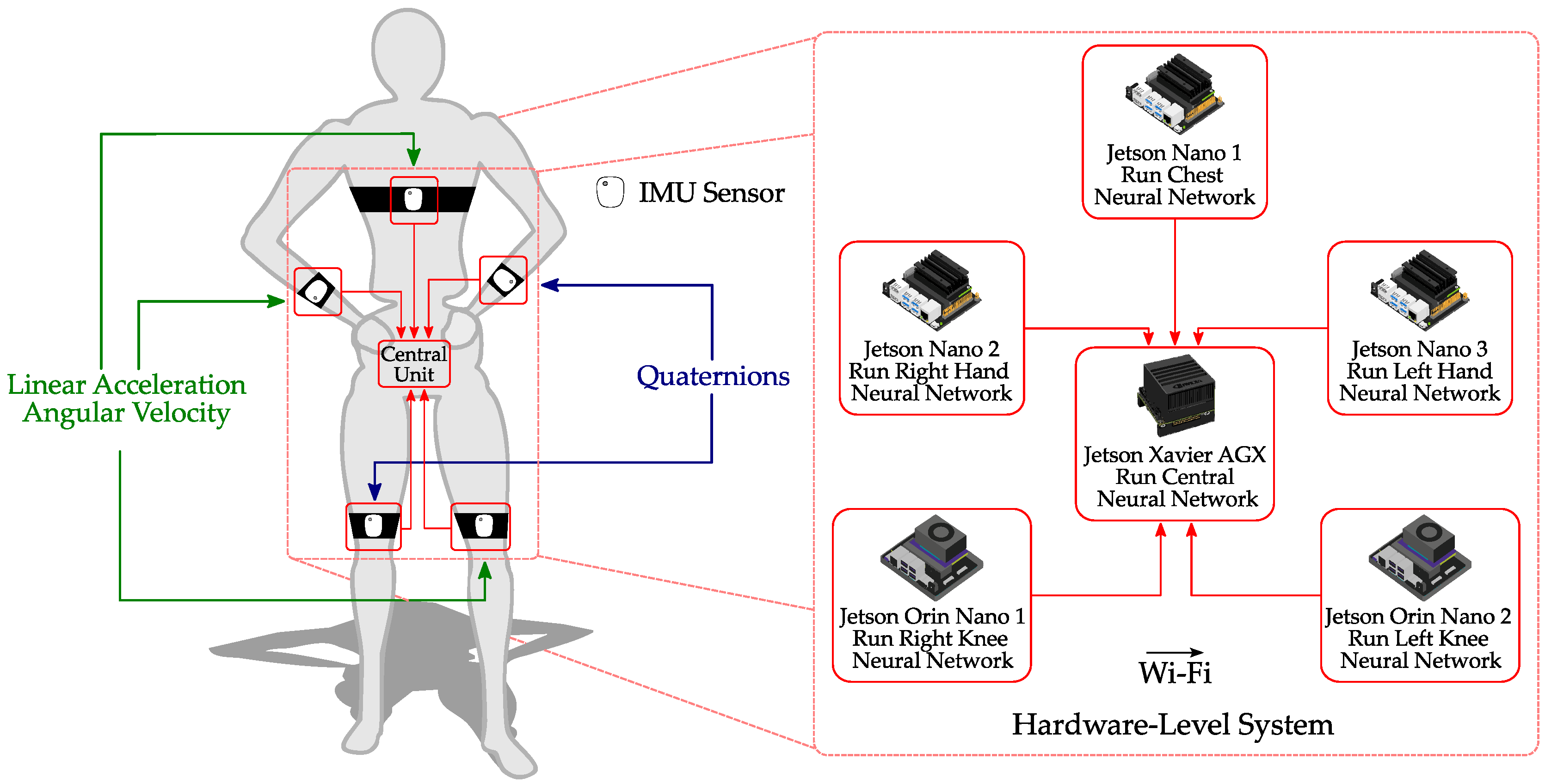
The sensors were placed on the chest, left hand, right hand, left knee, and right knee to capture complementary information from the torso and upper and lower limbs. The chest, left-knee, and right-hand nodes used corrected three-axis acceleration and angular-velocity signals, whereas the left-hand and right-knee nodes used quaternion orientation data. Figure 2 shows the wearable placements, sensing modalities, and associated embedded hardware.

Each wearable sensor communicated with its corresponding local node through BLE. The local nodes executed sensor-specific inference and transmitted class-probability vectors to the central node through the dedicated wireless network. The software organization, probability-message structure, communication protocol, synchronization strategy, and fallback operation are described in Section 3.

2.2. Neural Network Models

The neural network models were trained using the multi-sensor dataset reported in [2] and were based on the distributed CNN–LSTM architecture introduced in [36]. The trained models were integrated into the real-time framework without retraining during the live experiments.

Corrected acceleration and angular-velocity measurements were paired using their sensor timestamps to form six-dimensional samples [ax, ay, az, gx, gy, gz]. Quaternion measurements contained the four components [w, x, y, z] and were downsampled from 100 Hz to approximately 50 Hz by retaining samples separated by at least 20 ms. Each local node maintained a rolling buffer of the 50 most recent samples, corresponding to approximately 1 s under nominal operation. The three accelerometer–gyroscope nodes therefore used 50 × 6 inputs, whereas the two quaternion nodes used 50 × 4 inputs. Once the buffer was complete, the latest window was standardized using the sensor-specific scaler employed during training and evaluated at a target rate of 50 Hz; under nominal acquisition, consecutive windows differed by approximately one new sample.

All local nodes used the same CNN–LSTM structure, adapted only to the input dimensionality. The architecture comprised two one-dimensional convolutional layers with 16 output channels, kernel size 3, and padding 1, each followed by a rectified linear unit (ReLU) activation. A max-pooling layer with kernel size 2 reduced the temporal dimension before a single-layer LSTM with 32 hidden units. The final recurrent representation was processed by a 64-unit fully connected layer and a six-unit output layer. Softmax normalization produced the six-class vector transmitted to the central node and used directly as a fusion feature; no post-training probability-calibration procedure was applied. The accelerometer–gyroscope and quaternion models contained 9990 and 9894 trainable parameters, respectively.

Before experimental operation, each local model completed ten warm-up inference iterations. PyTorch v2.5.1 used graphics processing unit (GPU) acceleration through compute unified device architecture (CUDA) when available and otherwise reverted to central processing unit (CPU) inference.

At the central node, the five six-class probability vectors were concatenated in the fixed order chest, left knee, right hand, left hand, and right knee, producing a 30-dimensional fusion input. The central model consisted of a 64-unit fully connected layer with ReLU activation and dropout of 0.3, followed by a six-unit output layer. Softmax normalization generated the global class-probability vector. The central fusion model contained 2374 trainable parameters.

A real-time centralized reference configuration was also implemented using the same five physical wearable sensors and body placements. Unlike the distributed configuration, which used one sensing modality per local node and therefore comprised 26 input features, the centralized reference additionally used quaternion data from the chest sensor. Specifically, its input comprised acceleration and angular velocity from the chest, left knee, and right hand (18 features) together with quaternion data from the chest, left hand, and right knee (12 features), resulting in 30 features per sample. These measurements were combined into 50 × 30 temporal windows and processed directly by a single CNN–LSTM model on the central Jetson AGX Xavier. Thus, both configurations used the same five physical sensors but differed in processing placement and in the feature representation provided to the inference architecture.

The centralized CNN–LSTM consisted of three one-dimensional convolutional layers with 256 output channels, kernel size 3, and padding 1. Each convolutional layer was followed by batch normalization and ReLU activation, and the convolutional block was followed by max pooling with kernel size 2. The resulting sequence was processed by a two-layer LSTM with 256 hidden units. The final recurrent representation passed through fully connected layers of 128 and 64 units and a six-unit output layer, with dropout of 0.5 after the first fully connected layer. The centralized model contained 1,512,774 trainable parameters.

Table 3. List of activities classified by the HAR system in real time, with their labels and brief descriptions.

Activities	Label	Description
Sitting	0	A participant sitting on a chair
Folding Clothes	1	A participant folding clothes
Sweeping	2	A participant sweeping the floor
Walking	3	A participant walking at a moderate pace
Moving Boxes	4	A participant moving boxes between locations
Riding a Bike	5	A participant riding a stationary bicycle while seated

lists the activity classes considered in this work, together with their numerical labels and brief descriptions.

2.3. Participants, Experimental Protocol, and Robustness Scenarios

Ten adults participated in the real-time experiments, including eight men and two women. Their mean age was 25.4 ± 2.0 years, with a range of 22–29 years. None of these participants contributed data to the training or validation subsets used for model development; therefore, the real-time experiments constituted an independent evaluation on previously unseen participants.

Each participant performed Folding Clothes, Sweeping, Walking, Moving Boxes, and Riding a Bike once, for 2 min each. Sitting was performed for 1.5 min at the beginning of the experiment, after every two non-sitting activities, and at the end, resulting in approximately 16 min of labeled activity per participant. The order of the five non-sitting activities was randomized independently for each participant. Transition intervals were unlabeled and excluded from the classification analysis.

The total active recording duration also included transitions and minor experimental variations. Based on the recorded logs, the sessions lasted 17.08 ± 1.63 min per participant, with a range of 15.62–20.53 min.

In addition to normal operation, a controlled replay-based robustness analysis was conducted using the same preprocessing, sensor order, local CNN–LSTM models, and central fusion model. Perturbations were introduced at the local probability-stream level before central fusion, allowing the effect of unavailable local outputs to be evaluated without retraining the models.

For the random-loss scenarios, exactly 10% or 30% of the eligible probability vectors were independently suppressed in each local stream. Missing vectors were replaced using zero-order hold (ZOH), which retained the most recent valid probability vector until a new output became available. The loss masks were generated independently for the five streams to represent asynchronous message loss.

Temporary-disconnection scenarios introduced four non-overlapping outages per recording, each lasting 20–30 s. Single-node scenarios evaluated each local stream independently, while two-node scenarios evaluated all possible pairs of simultaneous disconnections. During each imposed outage, the replay analysis retained the last valid probability vector from the unavailable node, while the remaining nodes continued to provide updated outputs. This controlled protocol evaluated prolonged ZOH behavior independently of the live fallback implementation described in Section 3.2.

Each robustness condition was repeated using ten fixed random seeds. Results were first averaged across repetitions within each participant and were then summarized across the ten participants. This hierarchical procedure avoided treating the large number of overlapping temporal windows as statistically independent observations.

2.4. Evaluation Metrics

Classification performance was evaluated using pooled global accuracy, macro-averaged precision, recall, and F1-score, together with confusion matrices. Macro-averaging was selected because the number of valid predictions differed among activity classes. Unlabeled transition intervals were excluded. Metrics were also calculated independently for each participant and summarized using the mean, standard deviation (SD), and 95% bootstrap confidence interval (CI) obtained from 10,000 participant-level resamples.

Latency was calculated from the timing metadata carried by the local and global probability messages. Here, $t_0$ denotes the latest local-window reference timestamp used in a fusion event; $t_{\mathrm{l}\mathrm{a}\mathrm{s}\mathrm{t}\_\mathrm{l}\mathrm{o}\mathrm{c}\mathrm{a}\mathrm{l}\_\mathrm{s}\mathrm{e}\mathrm{n}\mathrm{d}}$ is the latest publication time among the local messages used by the central node; $t_{\mathrm{g}\mathrm{l}\mathrm{o}\mathrm{b}\mathrm{a}\mathrm{l}\_\mathrm{s}\mathrm{e}\mathrm{n}\mathrm{d}}$ is the publication time of the global prediction; and $t_{\mathrm{g}\mathrm{l}\mathrm{o}\mathrm{b}\mathrm{a}\mathrm{l}\_\mathrm{r}\mathrm{x}}$ is its reception time at the experiment manager.

$${\mathrm{L}}_{\mathrm{local}}={\mathrm{t}}_{\mathrm{last}\_\mathrm{local}\_\mathrm{send}}-{\mathrm{t}}_0$$

(1)

$${\mathrm{L}}_{\mathrm{fusion}}={ \mathrm{t}}_{\mathrm{global}\_\mathrm{send}}-{\mathrm{t}}_{\mathrm{last}\_\mathrm{local}\_\mathrm{send}}$$

(2)

$${\mathrm{L}}_{\mathrm{delivery}}={\mathrm{t}}_{\mathrm{global}\_\mathrm{rx}}-{\mathrm{t}}_{\mathrm{global}\_\mathrm{send}}$$

(3)

$${\mathrm{L}}_{\mathrm{e}2\mathrm{e}}={\mathrm{t}}_{\mathrm{global}\_\mathrm{rx}}-{\mathrm{t}}_0$$

(4)

The local stage includes local processing and probability-message publication. The fusion stage includes local-to-central delivery, synchronization waiting, fusion-input construction, central inference, and global-message preparation. The delivery stage represents transmission of the global prediction from the central node to the experiment manager. Therefore:

$${\mathrm{L}}_{\mathrm{e}2\mathrm{e}} = {\mathrm{L}}_{\mathrm{local}} + {\mathrm{L}}_{\mathrm{fusion}} +{ \mathrm{L}}_{\mathrm{delivery}}$$

(5)

The reported end-to-end latency characterizes post-window processing and does not include the initial time required to accumulate the 50 sensor samples. Its distribution was summarized using the mean; SD; median; 90th, 95th, and 99th percentiles; and maximum. Participant-level mean latency values were used to quantify between-participant variability and construct a 95% bootstrap CI.

Continuous-system throughput was defined as the number of global predictions generated per second. For participant $i$, the rate was calculated across all valid runs as:

$${\mathrm{R}}_{\mathrm{i}} = {\displaystyle \frac{{\sum }_{\mathrm{r}}({\mathrm{N}}_{\mathrm{i},\mathrm{r}}-1)}{{\sum }_{\mathrm{r}}({\mathrm{t}}_{\mathrm{i},\mathrm{r}}^{\mathrm{last}}-{\mathrm{t}}_{\mathrm{i},\mathrm{r}}^{\mathrm{first}})}}$$

(6)

where $N_{i,r}$ is the number of global predictions recorded during run $r$. Participant-level rates were summarized using the mean, SD, and 95% bootstrap CI.

Synchronization quality was evaluated using the synchronization span defined in Section 3.2, representing the temporal difference between the earliest and latest local probability messages accepted within the same fusion event. Only complete five-node groups accepted by the ATS were included. The distribution was summarized using the mean; SD; median; 90th, 95th, and 99th percentiles; and maximum.

Robustness was evaluated using accuracy and macro-F1-score. For each perturbed condition, results from the ten fixed seeds were first averaged within each participant. Participant-level values were then used to calculate the mean, SD, and 95% bootstrap CI obtained using the percentile method. Performance degradation was expressed as an absolute reduction in percentage points relative to the participant-level baseline. Bootstrap intervals were calculated using 10,000 resamples of complete participants.

Central-node power was recorded at approximately 1 Hz under centralized-processing and distributed-fusion configurations. The same central embedded device and measurement procedure were used in both cases. In the centralized configuration, the device executed the complete CNN–LSTM model; in the distributed configuration, it received synchronized local probability vectors and executed the fusion model.

For each valid power interval $i$, consumed energy was calculated as $E_i=P_i\Delta t_i$. Energy per global prediction was obtained independently for each run as:

$$E_{\mathrm{p}\mathrm{r}\mathrm{e}\mathrm{d}\mathrm{i}\mathrm{c}\mathrm{t}\mathrm{i}\mathrm{o}\mathrm{n}}={\displaystyle \frac{\sum _i{P}_i\Delta t_i}{\sum _i{N}_i}}$$

(7)

where $N_i$ is the number of global predictions produced during interval $i$. An idle-adjusted value was calculated using the measured baseline of $P_{\mathrm{i}\mathrm{d}\mathrm{l}\mathrm{e}}=5.417 \mathrm{W}$:

$$E_{\mathrm{idle-adjusted}}={\displaystyle \frac{\sum _i\mathrm{m}\mathrm{a}\mathrm{x}(P_i-P_{idle}, 0)\Delta t_i}{\sum _i{N}_i}}$$

(8)

Energy values were first calculated for each run and subsequently summarized using the mean, SD, and 95% bootstrap CI. Five centralized runs and ten distributed-system runs were included. These measurements characterize the central embedded node and not the aggregate energy consumption of all devices in the distributed architecture.

The centralized and distributed real-time configurations were compared using pooled classification performance, model complexity, communication representation, central-node power, and energy per prediction. Latency was also reported for both configurations; however, the centralized value was measured from reception of the latest sensor update at the host to completion of centralized inference, whereas the distributed value was measured from the local-window reference to reception of the global prediction. Consequently, the latency values were interpreted descriptively rather than as directly equivalent end-to-end measurements.

3. Proposed Real-Time Distributed Communication Framework

This section describes the proposed real-time communication framework and its implementation as a complete multi-sensor inference pipeline. Wearable sensors stream motion data to local embedded nodes, where sensor-specific preprocessing and neural inference are performed. The resulting outputs are transmitted to a central node, temporally synchronized, and fused to generate the global activity prediction during live operation.

The framework uses probability-level communication rather than transmitting complete raw-signal windows. Each local node publishes a timestamped softmax-normalized class-confidence vector that summarizes the activity evidence captured at its body location. These vectors are non-negative and sum to one, but they are used as neural-model confidence scores rather than independently calibrated posterior probabilities. The prototype was implemented using ROS Noetic as message-based publish–subscribe middleware; however, the architecture is applicable to other platforms that support timestamped communication, temporal alignment, and modular execution.

3.1. Real-Time Distributed Architecture and Inference Pipeline

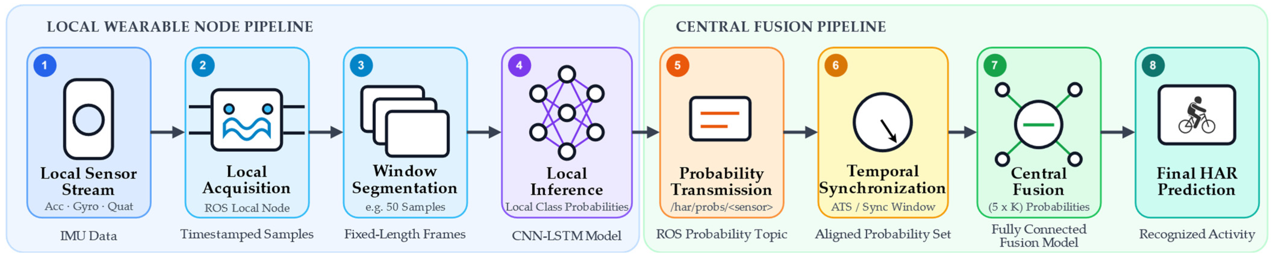
The system follows a three-layer architecture comprising wearable sensing, local inference, and central fusion. Each wearable sensor communicates through BLE with an embedded node assigned to a specific body location. The local node acquires and buffers the sensor stream, constructs temporal windows, applies the preprocessing used during training, executes its sensor-specific neural model, and publishes a timestamped class-confidence vector. The central node receives the five local outputs, verifies their temporal compatibility, concatenates them in a fixed sensor order, and executes the fusion model. 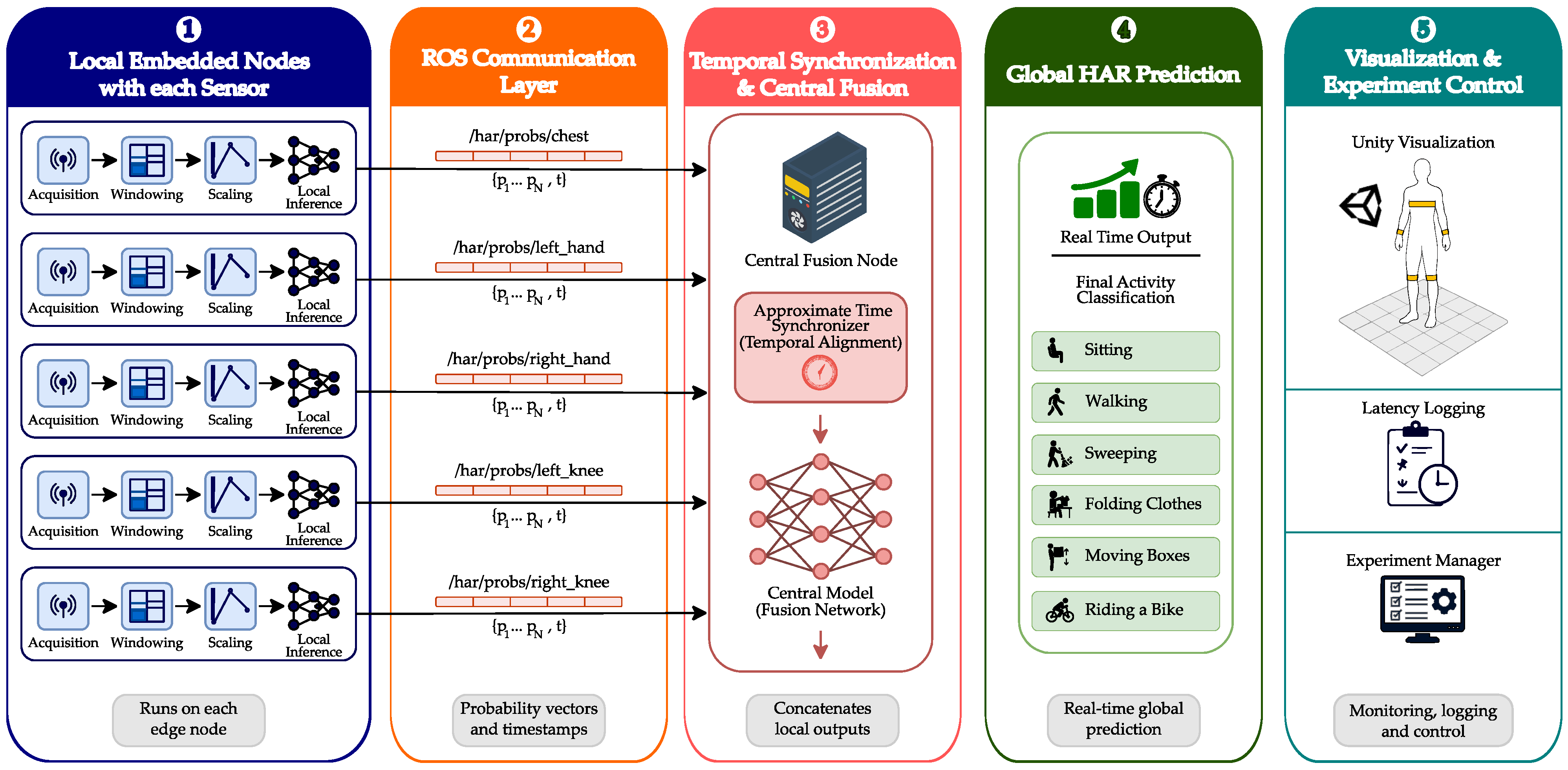Figure 3 presents this system-level organization, including the communication, prediction, visualization, and experimental-control components.

Unlike centralized processing, which transmits raw measurements for complete-window inference on one device, the proposed architecture performs the first inference stage locally and communicates compact model outputs. Each local node operates as a self-contained and causal inference unit: predictions are generated only from samples already received, without access to future measurements. Although the nodes use the same software sequence, they differ in sensor identifier, input features, trained model, and output topic. Figure 4 summarizes the corresponding processing sequence from local acquisition to final activity recognition.

After preprocessing, local node $i$ produces a logit vector that is converted into the softmax-normalized class-confidence vector:

$${\mathrm{p}}_{\mathrm{i}} = \left[{\mathrm{p}}_{\mathrm{i},1},{ \mathrm{p}}_{\mathrm{i},2}, \dots , {\mathrm{p}}_{\mathrm{i},\mathrm{K}}\right]$$

(9)

where $p_i$ is the output vector generated by local node $i$, $K$ is the number of activity classes, and $p_{i,k}$ is the softmax output assigned by node $i$ to class $k$. This local vector is used as an intermediate fusion feature rather than as the final system prediction; it summarizes the activity evidence captured at one body location.

For a system with N local nodes, the central fusion input is constructed by concatenating the synchronized local vectors:

$$\mathrm{P} = \left[{\mathrm{p}}_1,{ \mathrm{p}}_2, \dots , {\mathrm{p}}_{\mathrm{N}}\right]$$

(10)

where $P$ denotes the concatenated probability-level fusion input, N is the number of local nodes, and each $p_i$ is a $K$-dimensional vector. The resulting input therefore contains $N\times K$ values. In the implemented configuration, $N=5$ and $K=6$, producing a 30-dimensional fusion input. The synchronized vectors are arranged according to the fixed sensor order used during training:

$${\mathrm{x}}_{\mathrm{fusion}} = [{\mathrm{p}}_{\mathrm{chest}}, {\mathrm{p}}_{\mathrm{left}\_\mathrm{knee}}, {\mathrm{p}}_{\mathrm{right}\_\mathrm{hand}},{ \mathrm{p}}_{\mathrm{left}\_\mathrm{hand}},{ \mathrm{p}}_{\mathrm{right}\_\mathrm{knee}}]$$

(11)

Maintaining this order is essential because each segment of the fusion input is associated with a specific body location. An incorrect ordering would remain dimensionally valid but would be semantically inconsistent with the configuration used to train the central model. The central fusion model processes ${\mathrm{x}}_{\mathrm{fusion}}$ and generates the global class-confidence vector:

$${\mathrm{p}}_{\mathrm{global}} = [{\mathrm{p}}_{\mathrm{global},1},{ \mathrm{p}}_{\mathrm{global},2}, \dots ,{ \mathrm{p}}_{\mathrm{global},\mathrm{K}}]$$

(12)

The final predicted activity corresponds to the class with the highest value in the global output vector. Thus, the predicted label is obtained as:

$$\widehat{\mathrm{y}}= \mathrm{argmax}\left({\mathrm{p}}_{\mathrm{global}}\right)$$

(13)

where ${\mathrm{p}}_{\mathrm{global}}$ is the output probability vector generated by the central fusion model, and $\widehat{y}$ is the predicted activity label.

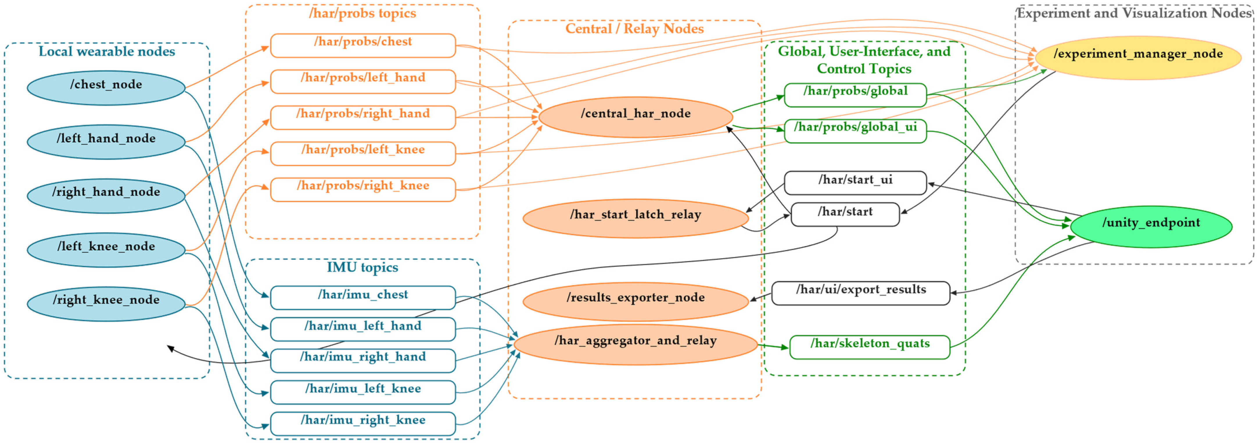
The software implementation follows a modular publish–subscribe organization. Sensor-specific nodes publish the local class-confidence streams, while independent modules perform central fusion, experiment control, logging, and visualization. Figure 5 shows the complete computation graph.

Table 4. Main communication channels used in the proposed real-time distributed HAR implementation.

Topic	Publisher	Subscriber	Purpose
/har/probs/chest	Chest Node	Central fusion node	Publish chest softmax vector
/har/probs/left_hand	Left-Hand Node	Central fusion node	Publish left-hand softmax vector
/har/probs/right_hand	Right-Hand Node	Central fusion node	Publish right-hand softmax vector
/har/probs/left_knee	Left-Knee Node	Central fusion node	Publish left-knee softmax vector
/har/probs/right_knee	Right-Knee Node	Central fusion node	Publish right-knee softmax vector
/har/probs/global	Central Fusion Node	Logger/Internal modules	Publish global prediction output
/har/probs/global_ui	Central Fusion Node	Unity interface	Publish global prediction for visualization
/har/start	Experiment Manager	Local and central nodes	Starts or stops the inference pipeline
/har/start_ui	Unity Interface	Experiment manager	Sends external start/stop commands

summarizes the principal communication channels. This separation allows prediction outputs to be logged or visualized without modifying local inference and permits the main modules to be tested independently.

3.2. Communication Protocol, Network Configuration, and Timestamp-Based Synchronization

The communication protocol defines how independently generated local outputs are transmitted and combined during real-time inference. Each local message contains six class-confidence values together with the metadata required for source identification, sequence tracking, synchronization, availability monitoring, and latency decomposition.

Table 5. Probability message structure used by the proposed real-time distributed HAR framework.

Name	Description
header.stamp	ROS publication timestamp used by ATS for message synchronization.
sensor_id	Identifies the source node or body location.
seq	Local sequence number of the published probability vector.
t0_ns	Timestamp of the latest sample in the local window; post-window latency reference.
t_send_ns	Local publication timestamp of the probability message.
t_last_local_send_ns	Latest local-message publication time used for fusion, stored in the global message.
K	Number of activity classes.
probs	Softmax-normalized class-confidence vector generated by the local model.
dropped_pct	Message-loss or availability indicator; set to 0 during normal live operation.

summarizes the implemented probability-message structure.

The fields serve two complementary purposes. During live inference, sensor_id identifies the source, header.stamp provides the ATS synchronization reference, and probs contains the local model output. The seq and dropped_pct fields support sequence and availability monitoring, while t0_ns, t_send_ns, and t_last_local_send_ns provide the temporal references required for post-experiment latency decomposition. The class count is stored in K. In all local nodes, header.stamp was assigned at probability-message publication using the synchronized ROS clock, t0_ns represented the most recent sensor sample in the corresponding local window, and t_send_ns represented the local publication time.

Reliable comparison of timestamps required stable network identities and a shared clock. The embedded nodes communicated through a dedicated local network and received fixed internet protocol (IP) addresses through dynamic host configuration protocol (DHCP) reservation [37]. The central device hosted the ROS master, while each local node was configured with the corresponding master uniform resource identifier (URI) and its own network address. Chrony synchronized the device clocks using the central node as the time reference [38]. These measures reduced configuration changes after reconnection and limited clock offsets that could otherwise cause outputs from similar motion intervals to appear temporally misaligned.

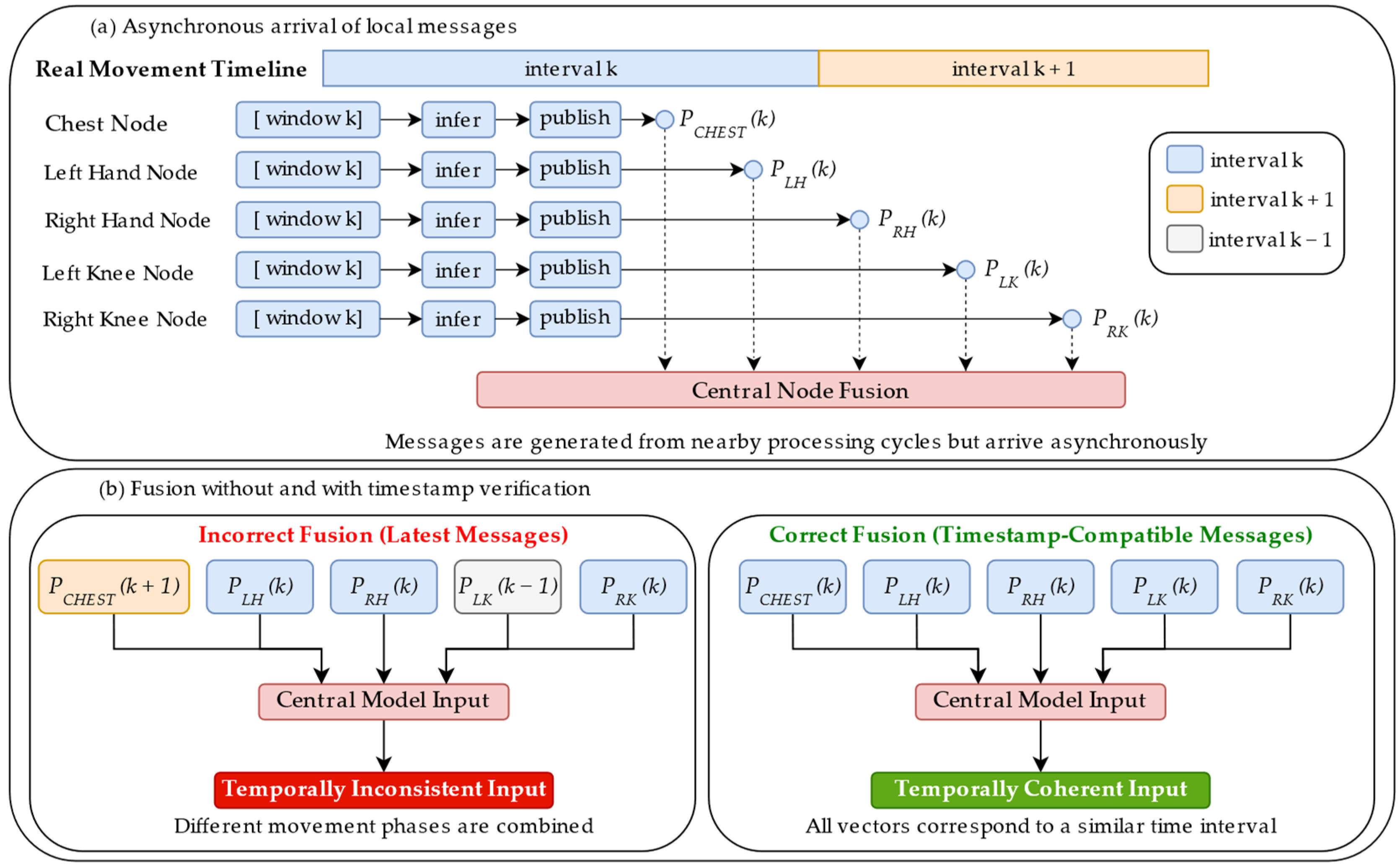
Despite the common time reference and experiment command, each node independently manages BLE acquisition, buffering, preprocessing, inference, and message publication. Small timing differences therefore arise from sensor streaming, local processing, network scheduling, and operating-system behavior. Figure 6 illustrates how using only the latest available message from each stream could combine outputs from different movement intervals, producing a complete but temporally inconsistent fusion input.

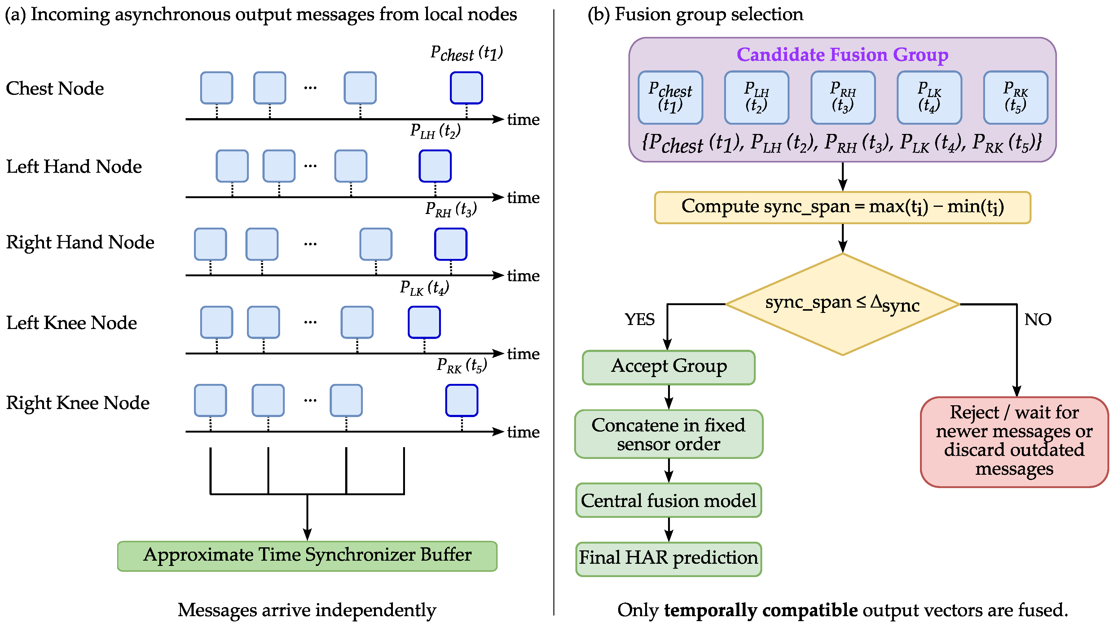
If the central node fused the latest available message from each local stream without timestamp validation, the resulting 30-dimensional input could combine outputs associated with different motion intervals. Such an input would be numerically complete but temporally inconsistent. The central node therefore uses an ATS to form a candidate group containing one message from each required local node:

$$\mathrm{G} = \left\{{\mathrm{p}}_1\left({\mathrm{t}}_1\right), {\mathrm{p}}_2\left({\mathrm{t}}_2\right), \dots , {\mathrm{p}}_{\mathrm{N}}\right({\mathrm{t}}_{\mathrm{N}}\left)\right\}$$

(14)

where ${\mathrm{p}}_{\mathrm{i}}\left({\mathrm{t}}_{\mathrm{i}}\right)$ is the class-confidence vector generated by the local node $\mathrm{i}$, and ${\mathrm{t}}_{\mathrm{i}}$ is the timestamp associated with that message. The temporal span of a candidate fusion group is calculated as the difference between the latest and earliest timestamps in the group. The group is accepted only if this span is within the configured synchronization tolerance:

$$\max \left({\mathrm{t}}_1,{\mathrm{t}}_2,\dots ,{\mathrm{t}}_{\mathrm{N}}\right)-\min ({\mathrm{t}}_1,{\mathrm{t}}_2,\dots ,{\mathrm{t}}_{\mathrm{N}}) \le {∆}_{\mathrm{sync}}$$

(15)

where ${∆}_{\mathrm{sync}}$ is the maximum synchronization tolerance. It was set to 50 ms in the implemented prototype, and ATS used a queue size of 10 messages per input stream.

A valid fusion group must therefore contain one message from every required node, satisfy the synchronization criterion, and follow the fixed sensor order expected by the central model. Accepted vectors are concatenated and processed by the fusion model; otherwise, ATS waits for newer messages or discards stale combinations according to its synchronization policy. If no complete five-node group is accepted by ATS for 350 ms, a watchdog activates fallback operation. Figure 7 summarizes this buffering, group-selection, and acceptance procedure.

During fallback operation, the central node continues generating predictions at 50 Hz using the most recent valid local vectors. Each cached vector is retained through ZOH for up to 2 s; if no update is received within that interval, the corresponding input is replaced by a uniform six-class vector. A 2 s startup grace period prevents premature fallback activation, and synchronized operation resumes only after ATS remains stable for 1 s. This live mechanism differs from the replay-based robustness analysis in Section 2.3, where the last valid vector was intentionally retained throughout each imposed 20–30 s disconnection.

The synchronization tolerance defines a trade-off between temporal consistency and prediction availability. A stricter tolerance improves alignment but may reduce accepted fusion groups, whereas a wider tolerance increases availability while permitting greater dispersion. The selected value considered the sampling frequency, window length, publication rate, and expected communication variability. For each accepted group, the system records the span between its earliest and latest timestamps, which is evaluated as the synchronization metric in Section 4.3.

3.3. Real-Time Visualization and Experimental Logging

The proposed system includes visualization and logging components for real-time monitoring and post-experiment analysis. These components subscribe to the prediction and timing outputs generated by the distributed pipeline without modifying the inference process. The central node publishes the global result through separate channels for experimental logging and the graphical interface, allowing inference to continue independently if the interface is disabled, modified, or replaced.

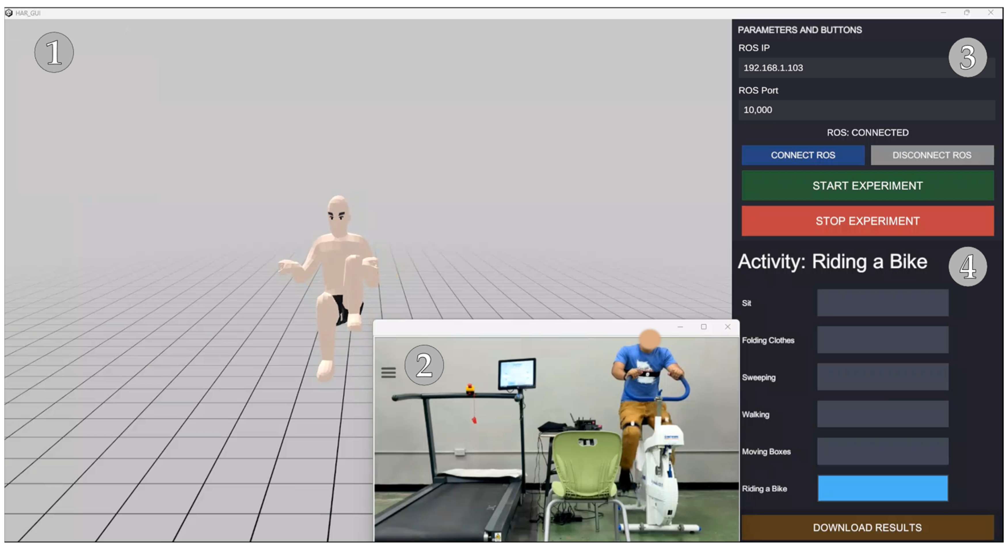
The graphical interface was implemented using Unity (editor version 2021.3.45f2; Unity Technologies, San Francisco, CA, USA) and connected to the distributed system through the local network. During each experiment, it displayed the global activity prediction and class-confidence values, mapped the numerical model output to the corresponding activity label, and provided connection parameters and start/stop controls. An avatar-based representation was also used to visualize the participant and wearable-sensor configuration.

The logging component recorded the local softmax vectors, global predictions, reference activity labels, sequence numbers, synchronization spans, and local and central timing measurements. These records provided the information required to calculate the classification, latency, throughput, and synchronization metrics reported in Section 4.

Together, the graphical interface and logging component supported live supervision and quantitative evaluation of the complete distributed HAR framework. The interface provided immediate feedback during execution, whereas the recorded outputs enabled reproducible post-experiment analysis of prediction performance and temporal behavior.

4. Results

This section reports classification, latency, throughput, and synchronization under normal operation; robustness under controlled probability-message loss and temporary node disconnections; communication payload; and the comparison between centralized and distributed real-time processing.

4.1. Real-Time Operation and Classification Performance

Figure 8 shows the graphical interface used to control the experiments and monitor the operation of the distributed HAR framework. The interface provided connectivity and start/stop controls, a participant-monitoring view, an avatar-based visualization, and the final activity prediction.

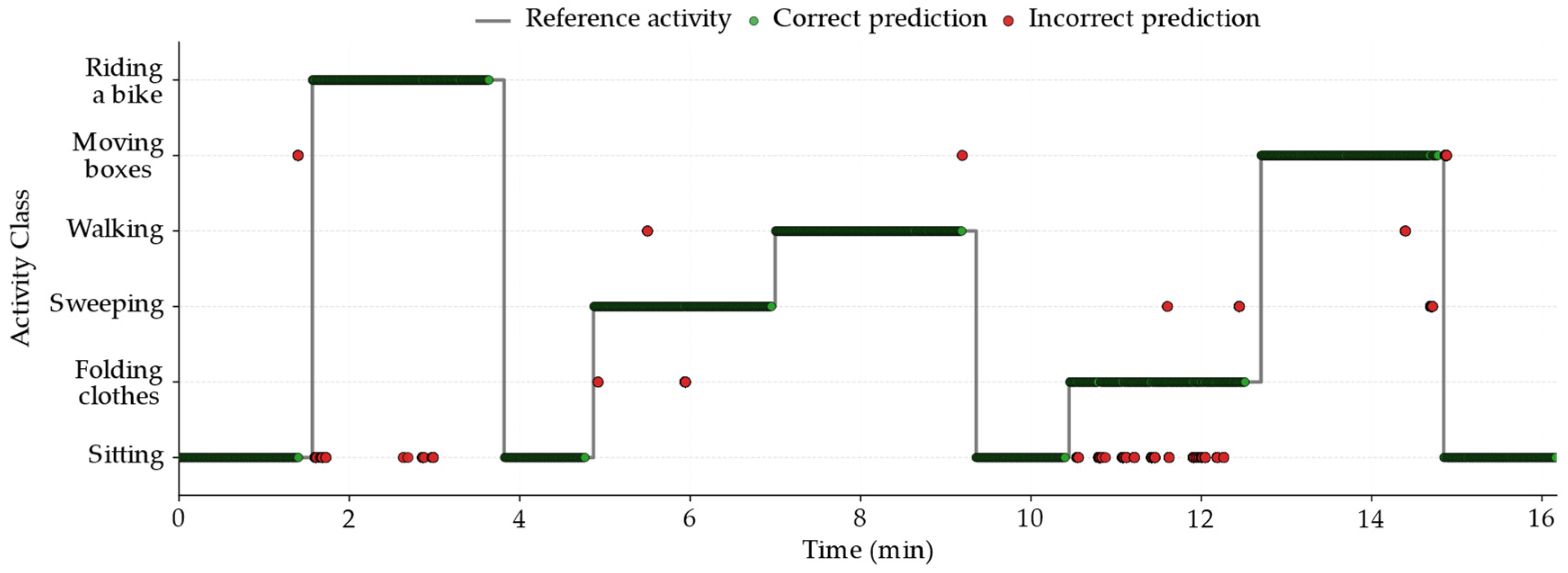
Continuous operation was verified using the recorded global outputs. Figure 9 compares the reference activity labels with the predictions generated during a representative experiment. Unlabeled transition intervals were excluded from the classification evaluation. The resulting sequence shows that the framework maintained a continuous prediction stream across the complete activity protocol, including changes between successive activity segments. This temporal record provides direct evidence of sustained online operation throughout the experimental session and illustrates how the global predictions followed the reference activity sequence over time.

Classification performance was evaluated using the reference activity labels and the predictions generated by the central fusion model. The predicted activity corresponded to the highest value in the global probability vector. The class distribution was imbalanced: Sitting accounted for 34.23% of the valid predictions, whereas each of the remaining activities represented between 12.39% and 14.07%. Macro-averaging was therefore used so that all six activities contributed equally to precision, recall, and F1-score.

Table 6. Pooled and participant-level classification performance of the real-time distributed HAR system.

Metric	Pooled Result (%)	Participant Mean ± SD (%)	95% Bootstrap CI (%)
Accuracy	95.868	95.767 ± 2.244	94.405–97.049
Macro-precision	96.066	96.183 ± 2.081	94.915–97.331
Macro-recall	95.277	95.207 ± 2.505	93.702–96.608
Macro-F1-score	95.642	95.509 ± 2.338	94.095–96.843

summarizes the pooled classification performance and participant-level variability, while the bootstrap CIs quantify the uncertainty associated with the participant-level estimates.

Table 7. Classification performance for each participant.

Participant	Valid Predictions	Accuracy (%)	Macro-F1-Score (%)
1	54,414	98.030	97.628
2	49,117	96.989	96.880
3	58,821	95.803	94.809
4	45,089	97.478	97.172
5	44,769	98.908	98.958
6	44,494	96.267	96.514
7	39,299	95.089	94.416
8	42,003	94.250	94.257
9	43,274	92.980	93.327
10	43,100	91.879	91.133

presents the participant-specific classification results and shows that performance remained consistently high across the cohort despite moderate inter-participant variability. Participant 5 achieved the strongest overall results, whereas Participant 10 obtained the lowest accuracy and macro-F1-score. Nevertheless, all participants exceeded 91% accuracy, indicating that the framework maintained reliable performance across previously unseen individuals. The similar variation observed in accuracy and macro-F1-score also suggests that the participant-dependent differences affected both overall correctness and class-balanced performance in a consistent manner. These results support the general stability of the distributed framework while also showing that individual movement patterns and activity-execution styles influenced classification performance.

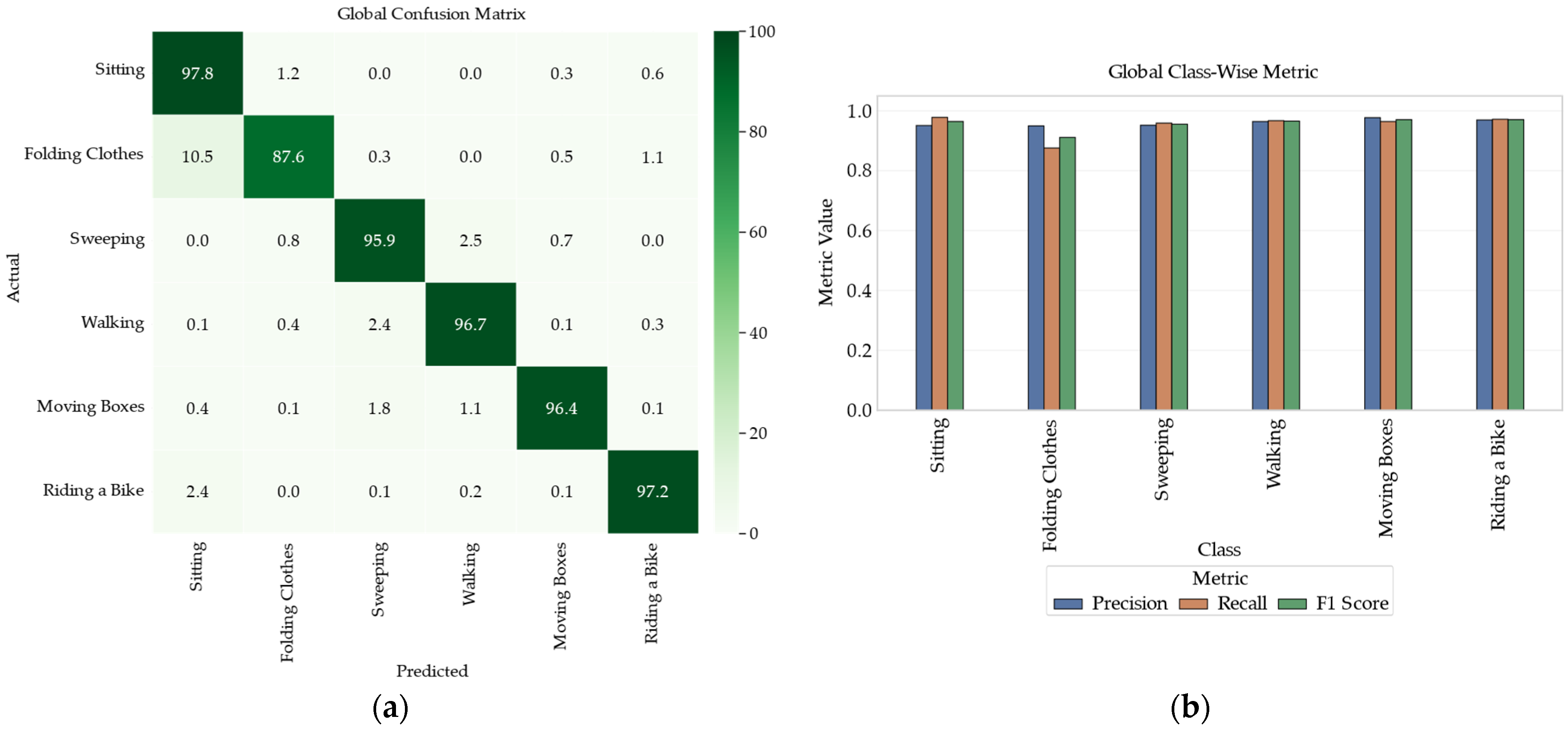
Figure 10 provides a class-level analysis of the aggregated predictions: panel (a) presents the row-normalized confusion matrix, and panel (b) compares precision, recall, and F1-score across the six activities.

Figure 10a shows that most predictions were concentrated along the main diagonal, with class recall ranging from 87.6% for Folding Clothes to 97.8% for Sitting. The dominant error was Folding Clothes being classified as Sitting, with 6173 cases (10.53%), whereas the reverse confusion occurred in only 1848 cases (1.16%). This error was concentrated mainly in Participant 9, who accounted for 40.39% of the Folding Clothes-to-Sitting misclassifications, followed by Participants 6 and 7 with 18.13% and 12.68%, respectively.

This asymmetry may result from seated folding intervals with limited torso and lower-limb motion, which can produce a global pattern similar to Sitting. In these cases, the most discriminative information is concentrated in the upper-limb sensors and may vary with the participant’s folding technique. Despite this confusion, Folding Clothes achieved an F1-score of 91.135%, while the pooled macro-F1-score remained at 95.642%.

4.2. Latency and Prediction Throughput Analysis

Latency and throughput were evaluated to characterize the temporal behavior of the complete distributed HAR pipeline during continuous execution. As defined in Section 2.4, post-window end-to-end latency begins at the reference timestamp of the available local input window and ends when the corresponding global prediction is received by the experiment manager. It includes local processing, local-to-central communication, synchronization, central fusion, and global-result delivery, but excludes the time required to accumulate the 50-sample window. Classification metrics were calculated from 464,380 predictions with valid activity labels, whereas the latency analysis included all 491,304 recorded global predictions.

Table 8. Post-window end-to-end latency and global prediction throughput during continuous real-time execution.

Metric	Value
Global predictions	491,304
Pooled latency mean ± standard deviation	33.963 ± 18.520 ms
Median latency	30.735 ms
90th percentile latency	45.568 ms
95th percentile latency	54.672 ms
99th percentile latency	113.687 ms
Maximum latency	418.505 ms
Predictions below 50 ms	93.217%
Participant-level mean latency ± standard deviation	33.788 ± 3.665 ms
95% CI of participant-level mean latency	31.755–36.059 ms
Mean prediction rate ± standard deviation	47.949 ± 1.926 predictions/s
95% CI of participant-level prediction rate	46.712–48.914 predictions/s
Participant-level prediction-rate range	43.019–49.032 predictions/s

summarizes the post-window latency distribution and prediction throughput across the ten participants. The pooled mean latency was 33.963 ms, while the lower median of 30.735 ms indicates a right-skewed distribution caused by occasional high-latency events. Although 93.217% of predictions were received within 50 ms, the upper percentiles and maximum value show that isolated timing outliers occurred during continuous execution. The 50 ms interval is therefore presented as a descriptive reference rather than a universal application-specific deadline.

Participant-level latency remained close to the pooled result, indicating limited variation among experimental recordings despite differences in their number of predictions. The system also generated 47.949 ± 1.926 global predictions/s, with participant-level rates ranging from 43.019 to 49.032 predictions/s. This sustained output rate remained close to the nominal operating target of 50 predictions/s, demonstrating that low single-prediction latency was maintained during continuous operation rather than only in isolated inference events.

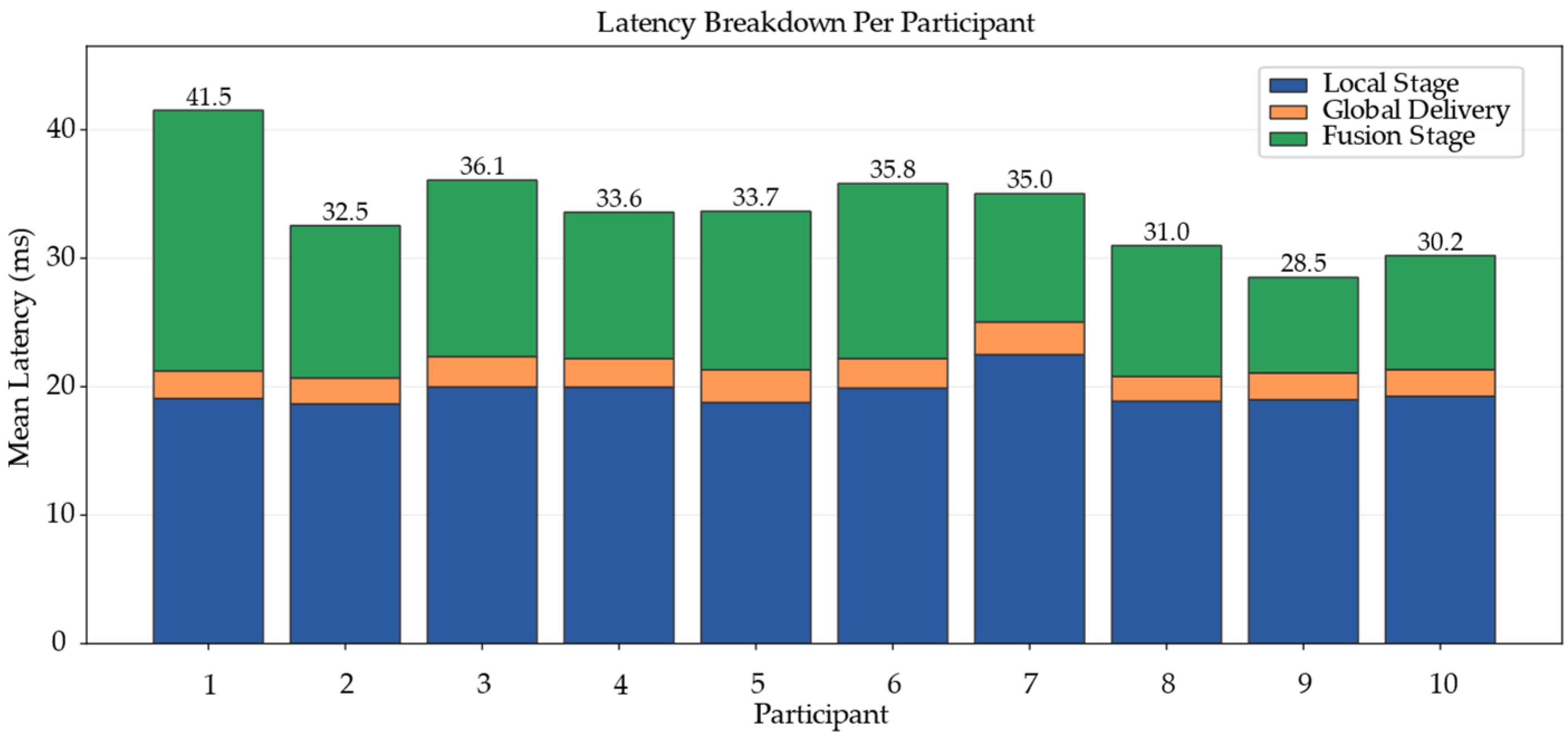
The complete post-window latency was divided into local, fusion, and global-delivery stages, with pooled means of 19.563, 12.182, and 2.219 ms, respectively. The local stage represented the largest contribution at approximately 57.6%, followed by the fusion stage at 35.9% and global delivery at 6.5%. Because the fusion stage includes local-to-central delivery, synchronization, fusion-input construction, central inference, and global-message preparation, it should not be interpreted as the execution time of the central neural network alone.

Figure 11 shows the mean contribution of each latency stage across participants. Despite inter-participant variation, local processing remained the dominant component and global delivery the smallest.

Overall, the results show that the framework sustained near-nominal prediction throughput while maintaining predominantly low post-window latency, although the observed upper tail confirms that mean values alone do not fully characterize temporal performance.

4.3. Synchronization Performance Under Normal Operation

Synchronization performance was evaluated using the complete five-node fusion groups accepted by the ATS during normal operation. The analysis included 442,220 events recorded in synchronized (SYNC) mode, compared with 491,304 global predictions in the latency analysis. Therefore, 49,084 predictions had no associated complete ATS record, consistent with outputs generated outside accepted synchronization callbacks, including predictions generated during fallback or other non-ATS publication intervals. Because the latency logs did not retain the fusion mode, these predictions could not be classified more precisely.

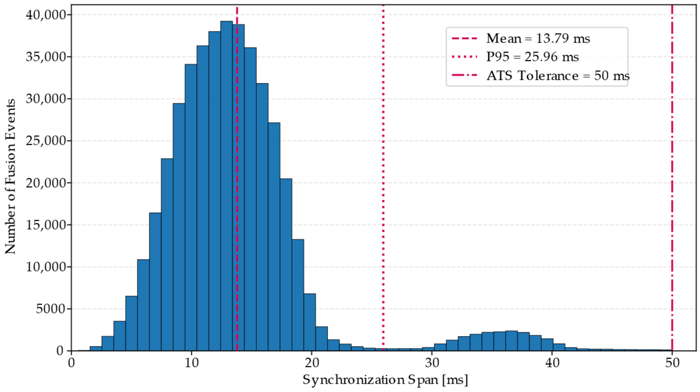
The accepted fusion groups had a mean synchronization span of 13.788 ± 6.381 ms and a median of 12.941 ms. The 90th, 95th, and 99th percentiles were 18.595, 25.958, and 38.905 ms, respectively, while the maximum span was 49.976 ms, remaining within the configured 50 ms tolerance. As shown in Figure 12, most events were concentrated at relatively low spans, with a smaller secondary concentration between 35 and 40 ms. This interval contained 2.35% of the accepted groups, while only 0.62% reached at least 40 ms and 0.17% reached at least 45 ms.

A retrospective threshold-coverage analysis showed that 24.88%, 93.25%, 95.26%, 99.38%, and 100% of the accepted events had spans not exceeding 10, 20, 30, 40, and 50 ms, respectively. Thus, a 20 ms threshold would cover most of the spans observed during normal operation, whereas a 10 ms threshold would be substantially more restrictive. However, because the logs contain only events accepted under the implemented 50 ms tolerance, these percentages cannot determine how alternative thresholds would affect prediction throughput, fallback activation, or classification performance.

The secondary concentration near 35–40 ms may reflect variability in local buffering, inference execution, message delivery, or operating-system scheduling, but the available logs do not allow these events to be attributed to a particular node or component. In addition, ATS did not expose candidate groups that were internally rejected before callback activation. The reported results are therefore restricted to complete accepted groups. Within this scope, the synchronization mechanism maintained measurable temporal consistency, with most fusion inputs showing substantially smaller temporal dispersion than the maximum permitted value.

4.4. Robustness Under Probability-Message Loss and Temporary Node Disconnections

Robustness was evaluated by introducing incomplete local probability streams before central fusion. The analysis included independent per-node probability-message losses of 10% and 30%, together with repeated temporary disconnections affecting one or two local nodes. Each recording contained four non-overlapping outages lasting 20–30 s, corresponding to 80–120 s of cumulative interruption. Missing outputs were replaced using the prolonged ZOH procedure described in Section 2.3, and each condition was repeated using ten fixed random seeds for all ten participants.

Table 9. Classification performance under controlled probability-message loss and repeated temporary node disconnections. pp denotes percentage points.

Condition	Accuracy Mean (%)	Accuracy SD (pp)	Accuracy 95% CI (%)	Macro-F1 Mean (%)	Macro-F1 SD (pp)	Macro-F1 95% CI (%)	Accuracy Drop (pp)
Baseline	95.87	1.29	95.03–96.98	95.57	1.44	94.53–96.82	—
Independent per-node message loss, 10%	95.33	1.27	94.45–96.32	94.99	1.48	93.94–96.19	0.54
Independent per-node message loss, 30%	94.31	1.37	93.25–95.35	93.90	1.70	92.49–95.17	1.55
Worst repeated single-node disconnection	92.37	3.56	89.12–94.61	91.92	3.70	88.59–94.37	3.50
Worst repeated two-node disconnection	88.78	8.12	81.46–93.62	88.07	8.38	80.56–93.35	7.09

summarizes participant-level accuracy and macro-F1-score under the evaluated conditions, including their variability, confidence intervals, and accuracy reduction relative to the replay-compatible baseline. Seeded repetitions were first averaged within each participant and then summarized across participants. The worst single- and two-node conditions correspond to the scenarios with the lowest mean participant-level accuracy. Because the baseline was calculated from the probability-stream records available for replay, it differs slightly from the complete normal-operation dataset reported in Table 6.

Independent message loss caused a gradual but limited performance reduction. Relative to baseline, accuracy decreased by 0.54 percentage points under 10% loss and by 1.55 percentage points under 30% loss, while macro-F1-score followed a similar pattern. These results indicate that retaining the most recent valid probability vector can preserve most of the classification performance when unavailable messages are intermittent and independently distributed among the local streams.

Repeated disconnections produced greater degradation because the retained vectors remained unchanged for longer intervals. The most critical single-node condition involved the left-hand quaternion stream, whereas the worst two-node condition simultaneously affected the right-hand accelerometer–gyroscope and left-hand quaternion streams. Accuracy decreased by 3.50 percentage points in the worst single-node scenario and by 7.09 percentage points in the worst two-node scenario, with participant-level variability also increasing substantially. The prolonged ZOH procedure therefore maintained a complete fusion input and allowed the replayed fusion pipeline to continue generating predictions. Nevertheless, it should be interpreted as a continuity mechanism rather than a substitute for current information from unavailable sensing locations.

4.5. Communication Payload Analysis

Communication payload was analytically evaluated using the implemented sensor configuration, window size, numerical representation, probability-message structure, and observed prediction rate. The comparison used complete-window transmission of the 26 features consumed by the five distributed local models as the communication reference. This reference is distinct from the 30-feature input used by the centralized real-time model.

Transmitting the five complete 50-sample local windows, comprising 26 features in total and represented using 32-bit floating-point values, would require 5200 bytes per fusion event. In contrast, the proposed framework transmits five six-class softmax vectors, corresponding to a numerical payload of 120 bytes per event. Probability-level communication therefore reduces the numerical payload by 97.69%. Moreover, the transmitted representation remains fixed at six values per node, independently of the local sensing modality and window length.

The complete ROS message also includes the header, source identifier, sequence number, timing metadata, class count, and message-availability information required for synchronization and traceability. Each serialized local message occupies approximately 89–94 bytes at the ROS application level, resulting in approximately 0.45 kB for a complete five-node set. At the observed mean rate of 47.95 predictions/s, the local probability streams generate approximately 21–23 kB/s of application-level traffic, excluding transport, network, and lower-layer protocol overhead.

Table 10. Calculated numerical and ROS application-level payload of the proposed probability-message protocol relative to complete raw-window transmission.

Metric	Value
Complete five-node local-window payload (26 features)	5200 bytes/fusion event
Five softmax vectors	120 bytes/fusion event
Numerical payload reduction	97.69%
Serialized local probability message	Approximately 89–94 bytes/message
Serialized five-node probability set	Approximately 0.45 kB/fusion event
Estimated application traffic at 47.95 predictions/s	Approximately 21–23 kB/s

summarizes the numerical and application-level payload characteristics. Overall, the proposed protocol replaces overlapping raw temporal windows with compact semantic messages containing a fixed-size six-value numerical representation while retaining the metadata required for source identification, temporal synchronization, fusion, and latency analysis.

4.6. Centralized and Distributed Real-Time Comparison

Both configurations used the same five wearable sensors and body locations but differed in processing placement and central input representation. The centralized system processed complete raw-feature windows using a single CNN–LSTM, whereas the distributed system performed sensor-specific local inference and transmitted probability vectors for central fusion. The comparison therefore evaluates different processing organizations using the same number of sensors and body locations.

Table 11. Real-time comparison of the centralized-processing and distributed-fusion configurations.

Metric	Centralized Processing	Distributed Fusion	Difference or Reduction
Physical wearable sensors	5	5	—
Central input	Raw-feature window	Five six-class probability vectors	—
Parameters executed at the central node	1,512,774	2374	99.84% reduction
Total deployed trainable parameters	1,512,774	52,132	96.55% reduction
Pooled accuracy (%)	95.084	95.868	+0.784 pp
Macro-F1-score (%)	95.139	95.642	+0.503 pp
Mean reported latency (ms)	19.800	33.963	Different boundaries
Mean central-node power (W)	8.624 ± 0.099	6.674 ± 0.423	22.6% reduction
Energy per prediction (J)	0.2925 ± 0.0118	0.1398 ± 0.0147	52.2% reduction
Idle-adjusted energy per prediction (J)	0.1087 ± 0.0030	0.0265 ± 0.0105	75.6% reduction

summarizes the classification, model-complexity, latency, and central-node energy results. The two configurations achieved similar classification performance, with slightly higher pooled accuracy and macro-F1-score in the distributed implementation. Because the metrics were calculated independently for each configuration, these differences are presented as descriptive results rather than as a paired statistical comparison. Because the centralized reference additionally includes the chest quaternion stream, the classification comparison should be interpreted as a system-level comparison between the implemented real-time architectures rather than as a strictly feature-matched ablation.

The principal architectural benefit was the substantial reduction in computational workload assigned to the central node. The smaller fusion model and the reduced central processing workload were accompanied by lower central-node power and energy per prediction. These measurements characterize only the central embedded node and do not establish an aggregate energy advantage for the complete distributed system.

The centralized reception-to-prediction latency was lower than the distributed post-window latency; however, the two measurements used different temporal boundaries. The distributed value additionally includes local processing, local-to-central communication, synchronization, central fusion, global publication, and delivery to the experiment manager. The latency values should therefore be interpreted descriptively rather than as a direct performance ranking. Within these boundaries, the distributed system maintained continuous real-time operation while substantially reducing central model complexity and energy demand.

5. Discussion

The results demonstrate that the proposed framework operates as a complete real-time distributed HAR system that integrates local inference, probability-level communication, temporal synchronization, central fusion, fallback operation, logging, and visualization. The following discussion examines its real-time feasibility, communication and robustness trade-offs, synchronization behavior, and principal limitations.

5.1. Real-Time Feasibility and Architectural Implications

The proposed system maintained continuous inference while coordinating five local embedded nodes and a central fusion node. It achieved a pooled accuracy of 95.868%, a macro-F1-score of 95.642%, a mean post-window end-to-end latency of 33.963 ms, and an average throughput of 47.949 predictions/s. These results show that the complete distributed pipeline operated close to its target rate of 50 Hz while preserving classification performance on participants whose data were not used for model training or validation.

The latency decomposition shows that the local stage was the largest measured component, accounting for approximately 57.6% of the mean post-window latency, followed by the fusion stage at 35.9% and global-message delivery at 6.5%. Because the fusion stage includes local-to-central message delivery, synchronization waiting, fusion-input construction, central inference, and global-message preparation, the present measurements do not fully separate network delay from synchronization and central processing. Therefore, optimization efforts should primarily target local processing, while future instrumentation should further decompose the fusion stage.

The centralized reference achieved similar classification performance, whereas the distributed design substantially reduced the model complexity and energy demand at the central node. Because the centralized and distributed latency measurements used different temporal boundaries, they are interpreted descriptively rather than as a strict head-to-head comparison.

5.2. Probability-Level Communication, Robustness, and Synchronization

Probability-level communication replaces complete raw-feature windows with fixed-size local softmax vectors. Under the complete-window transmission reference used in this study, this reduced the numerical payload per fusion event while providing the central fusion model with a fixed 30-value probability representation. The measured global-message delivery latency of 2.219 ms shows that delivery of the final prediction to the experiment manager represented a small fraction of the total post-window latency. Local-to-central probability-message delivery was included within the fusion stage and was not measured separately.

This representation also creates an information trade-off. Because the central node does not receive raw windows during distributed inference, the global prediction depends on the quality of the local classifiers and the ability of the fusion model to combine their outputs. The controlled robustness analysis showed limited degradation under independent random message loss: accuracy decreased by 0.54 percentage points at 10% loss and by 1.55 percentage points at 30% loss. Larger degradation occurred during simultaneous disconnection of informative node combinations, with the worst evaluated pair reducing accuracy by 7.09 percentage points. These findings indicate that probability-level fusion can tolerate moderate asynchronous losses but remains sensitive to prolonged unavailability of complementary sensing locations.

The local softmax outputs were used directly as fusion features and were not calibrated after training. Consequently, their numerical values should not be interpreted as calibrated posterior probabilities and may become overconfident under sensor degradation or operating conditions that differ from the training data. Temperature scaling, Monte Carlo dropout, confidence-aware weighting, and selective feature transmission are relevant extensions for improving uncertainty handling and fallback decisions.

Timestamp-based synchronization was necessary because the central model combines outputs produced independently by different devices. Across 442,220 accepted five-node fusion events, the mean synchronization span was 13.788 ms, with all accepted groups remaining within the configured 50 ms tolerance. This confirms that the vectors used for normal synchronized fusion were generally temporally close. However, the recorded synchronization log contains only ATS-accepted groups and does not expose rejected candidate combinations. Consequently, the retrospective threshold analysis cannot determine how alternative tolerances would affect prediction throughput, fallback activation, or classification performance.

5.3. Limitations and Future Work

Several limitations define the scope of the reported findings. First, the robustness experiments were conducted through controlled replay of previously recorded probability streams. Random message loss and temporary disconnections were imposed before central fusion, which isolates their effect on classification but does not reproduce all network-layer mechanisms associated with congestion, interference, retransmission, or clock instability. Future experiments should introduce controlled impairments directly into the live communication infrastructure.

Second, the study evaluated five sensors, six activity classes, and one participant at a time. For S sensors and K classes, the numerical probability payload and fusion-input dimension increase linearly as 4SK bytes and SK values per event, respectively. Additional sensing nodes may also increase synchronization waiting, queue occupancy, and fallback frequency. Simultaneous multi-user operation would require independent sensor groups, namespaces, synchronization queues, and fusion instances. This configuration was not evaluated in the present study.

Third, the current prototype depends on Jetson embedded platforms, a dedicated local network, BLE sensor links, and ROS-based message exchange. Although the framework is conceptually middleware-independent, its measured timing and reliability reflect this specific hardware and communication environment. Evaluating alternative middleware, wireless networks, embedded processors, and lower-power wearable platforms is necessary to establish broader generalizability across deployment settings.

Fourth, the energy comparison characterizes only the central Jetson AGX Xavier. The local inference nodes were not measured simultaneously; therefore, the reported reductions demonstrate lower central-node energy demand but do not establish that the complete distributed system consumes less aggregate energy than the centralized configuration. A future whole-system analysis should jointly measure sensing, local inference, communication, and central fusion energy.

Fifth, the implemented fusion model was not compared experimentally with latest-message fusion without timestamp validation, simple probability averaging, confidence-weighted averaging, or models trained under different synchronization tolerances. These ablations would help isolate the contribution of learned fusion and temporal alignment and should be included in future evaluations.

Finally, although the ten real-time participants were independent of those used for model development, the cohort was limited in size and demographic diversity. Additional participants, longer recordings, broader activity sets, variable activity intensities, and unconstrained environments are required to evaluate generalization beyond the controlled protocol used in this study.

6. Conclusions

This work presented a real-time distributed HAR framework that integrates local CNN–LSTM inference, timestamped probability-level communication, approximate synchronization, fallback operation, central fusion, logging, and visualization. The system was evaluated with five wearable sensors and ten participants whose data were not used for model training or validation.

The framework achieved 95.868% accuracy and a 95.642% macro-F1-score. It sustained 47.949 predictions/s, with a mean post-window end-to-end latency of 33.963 ms and a mean synchronization span of 13.788 ms. Under 30% independent probability-message loss, accuracy remained at 94.31%, whereas the worst simultaneous two-node disconnection reduced accuracy to 88.78%. Probability-level communication reduced the numerical payload by 97.69% relative to complete-window transmission, and central-node energy per prediction decreased by 52.2% relative to centralized real-time processing.

These findings support the feasibility of synchronized distributed wearable inference while defining its principal trade-offs. Future work should evaluate live network impairments, whole-system energy consumption, alternative fusion and synchronization strategies, calibrated uncertainty estimates, lower-power hardware, and broader participant and activity cohorts.