Improving Cross-Organ Generalization in Histopathology Segmentation via Evidence-Guided Vision–Language Query Decoding

Abstract

Domain shift remains a major obstacle to robust histopathology image segmentation, especially when models trained on several source organs are deployed to unseen anatomical sites. This study addresses cross-organ adenocarcinoma segmentation by introducing an evidence-guided vision–language segmentation framework that incorporates pathology-relevant morphological evidence into dense mask prediction. The proposed method uses a pathology vision–language encoder to extract image and text representations, a Semantic Query Booster to form image-aware segmentation queries, and an evidence-guided query recalibration that integrates positive tumor-supporting evidence and negative misleading evidence. Experiments were conducted on cross-organ adenocarcinoma datasets from the COSAS challenge under a source-only domain generalization setting, with colorectum, stomach, and pancreas as source domains and ampullary, gallbladder, and intestine as unseen target domains. The proposed framework achieved the highest pooled performance on the seen, unseen, and overall evaluation sets among the compared segmentation, domain generalization, and foundation model-based systems. These findings support the use of structured pathology evidence for cross-organ tumor segmentation under source-only training.

1. Introduction

Computational pathology has become an important tool for quantitative cancer analysis, biomarker assessment, and computer-assisted diagnosis. Despite recent progress, robust deployment of pathology segmentation models remains challenging because histopathological images can vary substantially across staining protocols, scanners, tissue preparation procedures, and acquisition conditions. In addition to these technical variations, organ-associated domain shift has attracted increasing attention. Tumors from different anatomical sites may belong to the same pathological category but still present distinct glandular architecture, stromal composition, tissue context, nuclear density, and tumor–stroma interfaces [1]. Therefore, domain generalization (DG), which aims to learn models from source domains that can generalize to unseen target domains without accessing target-domain data during training, is particularly important for cross-organ pathology segmentation [2,3].

Existing DG methods for pathology segmentation are largely organized around two paradigms: style augmentation and domain-invariant representation learning. Style-based approaches expand the source-domain distribution by perturbing color, texture, stain appearance, and other low-level visual factors, whereas feature alignment approaches reduce inter-domain discrepancy by enforcing more compact or domain-invariant representations. Although these methods are effective for appearance-driven shifts, they are less suited to cross-organ adenocarcinoma segmentation, where domain variation is tightly coupled with organ-specific morphology. Variations in glandular architecture, stromal composition, epithelial organization, nuclear density, and tumor–stroma interfaces constitute diagnostic structures rather than nuisance style. Consequently, aggressive feature alignment can attenuate discriminative morphological patterns, while appearance-level augmentation provides limited coverage of structural heterogeneity across organs [4].

Pathology foundation models offer a natural way to incorporate prior knowledge into cross-domain segmentation. Recent histopathology encoders and vision–language models, such as UNI, PLIP, and CONCH, learn representations from large-scale tissue images or image-text pairs and have shown strong transferability across downstream pathology tasks [5,6,7]. For cross-organ adenocarcinoma segmentation, this form of semantic grounding is relevant because the target category is shared across organs, while the surrounding tissue context and morphological presentation may vary across anatomical sites [1]. However, semantic grounding at the image or category level is still not sufficient for dense cross-organ segmentation. A category prompt can indicate that the target is adenocarcinoma, but does not specify which morphological cues should guide pixel-level mask prediction when the same tumor category appears in a new organ domain. In such cases, the model should distinguish tumor regions from surrounding tissue using local evidence, including glandular organization, epithelial crowding, luminal distortion, stromal reaction, and tumor–stroma boundaries. These cues are more specific than a class label and are also closer to the visual evidence needed by a segmentation decoder.

This motivates an evidence-guided formulation of pathology vision–language segmentation. We construct a structured pathology evidence bank that describes tumor-related morphology and misleading visual patterns. Positive evidence describes adenocarcinoma-related morphology, including irregular gland formation, epithelial crowding, luminal distortion, stromal reaction, and tumor–stroma boundaries. Negative evidence identifies potentially unreliable patterns caused by artifacts, acquisition-dependent appearance variations, or synthetic-looking shortcuts. This separation provides a more specific semantic prior for cross-organ segmentation while preserving the source-only setting.

In this work, we study cross-organ adenocarcinoma segmentation from the perspective of evidence-guided source-domain learning. The central idea is to make the segmentation decoder depend less on organ-specific appearance and more on pathology evidence that remains meaningful across organs. To this end, we design a source-only vision–language framework with three coupled components. First, class-domain text embeddings are used to construct image-aware decoder queries from dense image–text similarity responses. Second, a source-derived pathology evidence bank is introduced into query-based mask decoding. The evidence-guided decoder then introduces source-derived positive morphology through cross-attention and applies a positive–negative ranking loss only to tumor-matched queries. Third, a text-conditioned feature–style regularization branch perturbs intermediate visual features during training, reducing the tendency of the decoder to fit source-domain style patterns. The main contributions of this work are summarized as follows:

• We propose a source-only evidence-guided vision–language segmentation framework that constructs image-aware segmentation queries from dense visual features and class-domain textual context.
• We develop an evidence-guided decoding and feature–style regularization strategy for source-domain learning. Positive and negative pathology evidence are incorporated into query-based mask decoding, while text-conditioned style perturbation adds feature-level variation during training.
• Experiments on cross-organ adenocarcinoma segmentation show that the proposed method achieves state-of-the-art performance compared with representative segmentation and domain generalization baselines.

2. Related Work

2.1. Domain Generalization in Computational Pathology

Domain generalization (DG) aims to learn models from one or multiple source domains that remain reliable on unseen target domains without accessing target-domain data during training. This setting is particularly relevant to computational pathology, where deployment environments are difficult to enumerate in advance and histopathological images exhibit substantial distribution shifts across laboratories, scanners, staining protocols, tissue preparation procedures, and patient cohorts [2,3]. Unlike domain adaptation, which usually assumes access to target-domain samples during adaptation, DG requires the model to acquire transferable representations solely from the source-domain data. This requirement makes DG clinically important for pathology segmentation, since models trained in one set of institutions or acquisition conditions are expected to operate robustly in unseen diagnostic settings.

A major body of work in computational pathology addresses domain shift through stain normalization, stain augmentation, style perturbation, and domain-invariant representation learning. Stain normalization reduces color variability by mapping images to a standardized stain appearance, whereas stain or style augmentation expands the training distribution by synthesizing plausible appearance variations [8,9,10,11]. More recent methods further improve robustness by learning stain-generalizable or domain-agnostic representations through meta-learning, contrastive learning, adversarial learning, or feature regularization [3,12]. These approaches have established that appearance-level variability is a critical source of generalization error in pathology models and that carefully designed augmentation or representation learning strategies can improve robustness across staining and scanner conditions.

Despite this progress, cross-organ pathology segmentation presents a more complex form of domain shift. Evidence from recent domain generalization benchmarks shows that histopathology models suffer from performance degradation when evaluated across different scanners, laboratories, tumor types, species, and tissue morphologies [13,14]. In cross-organ adenocarcinoma segmentation, the target shift is not limited to color or scanner-induced appearance changes; it is coupled with organ-specific glandular architecture, stromal composition, epithelial organization, nuclear density, and tumour–stroma interfaces [1]. Therefore, methods that primarily normalize stain appearance or enforce compact domain-invariant features provide only a partial solution. Over-constraining domain variation risks attenuating diagnostically relevant morphology, whereas appearance-level augmentation provides limited coverage of organ-level structural heterogeneity. These limitations motivate DG strategies that preserve pathology-specific semantic structures while explicitly improving the stability of dense visual features under unseen-organ shifts.

2.2. Vision–Language Foundation Models for Pathology

Foundation models have recently reshaped representation learning in computational pathology. Large-scale self-supervised pathology encoders such as UNI and Prov-GigaPath have demonstrated that pretraining on massive histopathology image collections can produce transferable visual representations across diverse downstream tasks [5,15]. These models reduce the dependence on task-specific annotations and provide strong initialization for classification, retrieval, survival prediction, and tissue-level analysis. However, image-only foundation models primarily learn visual regularities from histology images and do not explicitly incorporate the textual knowledge that pathologists use to describe tumor morphology, tissue organization, and diagnostic criteria.

Pathology vision–language models further extend this paradigm by aligning histopathological images with biomedical textual semantics. PLIP introduced pathology language–image pretraining using image–text pairs collected from public pathology resources, enabling zero-shot classification and image-text retrieval in pathology [6]. CONCH further scaled contrastive image caption pretraining with diverse histopathology images, biomedical text, and more than one million image caption pairs, showing strong transferability across multiple computational pathology benchmarks [7]. By mapping histology images and pathology descriptions into a shared semantic space, these models can provide semantic anchors for concepts such as glandular formation, epithelial organization, stromal reaction, tumor morphology, and tissue context. Such semantic priors are particularly valuable for cross-organ adenocarcinoma segmentation, where tumor-related structures need to be recognized across unseen anatomical environments.

Despite their promise, existing pathology vision–language models are still mainly used for classification, retrieval, zero-shot recognition, captioning, or general representation learning. Their application to dense prediction and domain-generalized segmentation remains less explored. Recent work such as PathVLG has shown that vision–language guidance can improve domain generalization for cross-organ adenocarcinoma segmentation by refining segmentation queries and enriching style representations [16]. Nevertheless, semantic alignment alone does not explicitly regulate the feature-level variations that affect dense mask prediction. In particular, stain variability, scanner response, tissue preparation artifacts, compression noise, and organ-specific tissue backgrounds can introduce unstable spectral patterns into intermediate visual features. Therefore, pathology vision–language segmentation requires not only high-level semantic grounding but also feature-level calibration mechanisms that stabilize dense representations under unseen domain shifts.

2.3. Language Descriptions for Visual Recognition and Segmentation

Recent studies have shown that vision–language models can benefit from textual inputs that describe visual appearance more explicitly. CoOp learns continuous prompt tokens for CLIP-like models and reduces dependence on manually written prompt templates [17]. Menon and Vondrick used large language models to generate visual attributes for image classification [18], while CuPL generates customized prompts with large language models to improve zero-shot recognition [19]. These studies suggest that descriptive language can provide visual cues that are not available in a simple class prompt.

Medical segmentation has also begun to use richer textual input. FLanS provides free-form language-based segmentation in medical images, while SAT relies on a large-vocabulary medical segmentation model driven by text prompts [20,21]. Although these methods expand the role of text in segmentation, most still use language to specify the target object or anatomical region. In cross-organ adenocarcinoma segmentation, the more difficult question is which tumor-related cues remain reliable across organs. For this reason, we organize pathology descriptions into positive and negative evidence and use them to recalibrate query representations during mask decoding.

2.4. Generative and Feature–Style Regularization for Domain Generalization

A separate line of DG research increases source-domain diversity through image- or feature-level perturbation. L2A-OT learns pseudo-novel domains for domain generalization [22]. MixStyle mixes feature statistics between training samples to synthesize implicit feature styles [23]. In semantic segmentation, Fourier domain adaptation shows that low-frequency appearance statistics can strongly affect cross-domain transfer [24]. These methods support a common observation, namely, that models trained on limited source domains can often benefit from controlled style variation provided that semantic content is preserved.

This issue is pronounced in pathology, where stain intensity, scanner response, blur, tissue preparation, and synthetic-image artifacts can change appearance without changing the tumor label. At the same time, morphology cannot be treated as a removable style factor because gland shape, stromal organization, and tumor boundaries are part of the diagnostic signal.

3. Methodology

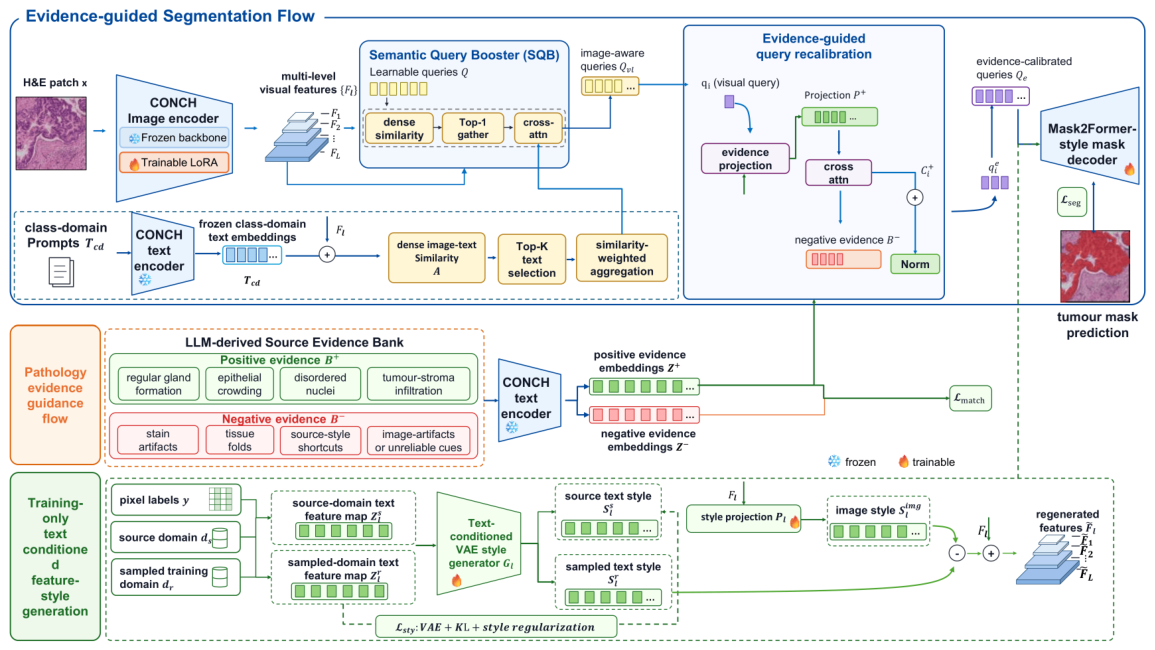
As shown in Figure 1, we propose a source-only evidence-guided vision–language segmentation framework with vision–language query construction, evidence-guided query decoding, and text-conditioned feature–style regularization. The Semantic Query Booster (SQB) forms image-aware decoder queries from multi-level visual features and source-domain class embeddings. Positive pathology evidence then recalibrates these queries prior to mask decoding, while positive and negative evidence jointly constrain tumor-matched decoder queries during training. The feature–style branch introduces source-domain appearance variation at intermediate feature levels without altering the inference pathway.

3.1. Problem Formulation

Let $\mathcal{S}=\{{\mathcal{D}}_1,{\mathcal{D}}_2,\dots ,{\mathcal{D}}_M\}$ denote M source organ domains, where each source domain ${\mathcal{D}}_m$ contains annotated histopathology patches:

$${\mathcal{D}}_m={\left\{(x_i^m,y_i^m)\right\}}_{i=1}^{N_m}$$

(1)

where $x_i^m$ is a histopathology patch and $y_i^m$ is its tumor segmentation mask. The unseen target domain ${\mathcal{D}}_t$ is unavailable during training. The expected target risk is

$${\mathcal{R}}_t\left(f_{\theta }\right)={\mathbb{E}}_{(x,y)\sim {\mathcal{D}}_t}\left[{\mathsf{\ell }}_{\mathrm{seg}}(f_{\theta }\left(x\right),y)\right].$$

(2)

Since ${\mathcal{D}}_t$ is inaccessible during training, the model is optimized on the empirical source risk:

$${\mathcal{R}}_s\left(f_{\theta }\right)={\displaystyle \frac{1}{M}}{\displaystyle \sum _{m=1}^M}{\mathbb{E}}_{(x,y)\sim {\mathcal{D}}_m}\left[{\mathsf{\ell }}_{\mathrm{seg}}(f_{\theta }\left(x\right),y)\right].$$

(3)

The target risk can be decomposed as

$${\mathcal{R}}_t\left(f_{\theta }\right)={\mathcal{R}}_s\left(f_{\theta }\right)+{\Delta }_{\mathrm{DG}}(f_{\theta };\mathcal{S},{\mathcal{D}}_t),$$

(4)

where ${\Delta }_{\mathrm{DG}}$ denotes the generalization gap between the source organs and the unseen target organ.

We augment the source-domain objective with pathology evidence guidance and text-conditioned feature–style regularization. For each non-empty source-domain tumor mask, the matching step selects the final decoder query that maximizes the product of its tumor class confidence and soft mask overlap. The evidence constraint is evaluated only on these tumor-matched queries, and is denoted by ${\mathcal{L}}_{\mathrm{match}}$. The training objective is

$$\underset{\theta }{min}{\mathcal{R}}_s\left(f_{\theta }\right)+{\lambda }_{\mathrm{match}}{\mathcal{L}}_{\mathrm{match}}+{\lambda }_{\mathrm{sty}}{\mathcal{L}}_{\mathrm{sty}}.$$

(5)

3.2. Vision–Language Query Construction

The purpose of this module is to make the decoder queries depend on the current image content before pathology evidence is introduced. Given an input patch x, the pathology vision–language encoder extracts multi-level visual features ${\left\{F_l\right\}}_{l=1}^L$. The text encoder maps class-domain prompts into fixed text embeddings:

$$T_{\mathrm{cd}}={\left\{t_{r,c}\right\}}_{r,c}\in {\mathbb{R}}^{N_{\mathrm{cd}}\times D},$$

(6)

where r indexes the domain prompt and c indexes the segmentation class. The embeddings are normalized before computing the similarity. SQB updates learnable decoder queries using dense image–text responses. A visual feature map is first projected into the text embedding space and reshaped into dense visual tokens:

$$V=Proj\left(F\right)\in {\mathbb{R}}^{B\times HW\times D}.$$

(7)

The dense image–text similarity is computed as

$$A=V{\overline{T}}_{\mathrm{cd}}^{\top },$$

(8)

where ${\overline{T}}_{\mathrm{cd}}$ denotes normalized text embeddings. For each visual token, the top-K related text embeddings are selected from A. The similarity response and gathered embeddings are projected as

$$S_{\mathrm{sim}}=W_{\mathrm{sim}}A,S_{\mathrm{aggr}}=W_{\mathrm{aggr}}\mathrm{TopK}(A,T_{\mathrm{cd}}).$$

(9)

The learnable query set Q is updated through two cross-attention operations:

$$Q_{\mathrm{vl}}={\mathrm{CA}}_{\mathrm{aggr}}\left({\mathrm{CA}}_{\mathrm{sal}}(Q,S_{\mathrm{sim}}),S_{\mathrm{aggr}}\right).$$

(10)

The resulting $Q_{\mathrm{vl}}$ is used as the image-aware query representation.

3.3. Evidence-Guided Query Decoding

The evidence bank was constructed from the 180 training patches of the three source organs. Each H&E patch was paired with a translucent tumor mask overlay so that the generated description referred to the annotated target region. The evidence statements were generated through the OpenAI web interface using the same fixed structured instruction, rather than being manually written by pathologists. The instruction and JSON output schema were applied to every contact sheet. OpenAI ChatGPT (GPT-5.5) web interface (accessed on 7 July 2026) was used only during offline construction of the evidence bank, and was not called during model training or inference. The complete instruction and schema are provided in Supplementary Material S1.

The task-defining instruction is summarized below:

“Use the mask only to identify the segmentation target. Do not infer tumour grade, stage, prognosis, or molecular status. Do not use organ identity, stain darkness, scanner brightness, blur, compression, background colour, or image artifacts as positive evidence. Focus on stable morphology that may transfer across hospitals, stains, scanners, and organs. Return strict JSON containing target-region morphology, tumour-stroma interface, gland and lumen structure, cellularity, stable positive evidence, domain-style evidence to ignore, artifact or unreliable evidence, and negative shortcut evidence.”

The 180 sample-level records were screened at the record level. A record was eligible when it could be parsed as a JSON object and was neither labeled exclude nor assigned usable_for_training=false. A total of 137 records met these conditions, comprising 127 usable and 10 uncertain records. The remaining 43 records were excluded.

Positive candidates were collected from the target-region morphology, tumor–stroma interface, gland–lumen structure, cellularity, and stable positive evidence fields. Statements referring to staining, scanners, blur, annotations, organ identity, or other appearance factors were removed. Negative candidates were restricted to domain style and artifact-related fields, and were rejected when they contained tumor morphology or annotation terms.

After exact deduplication, quality-prioritized round robin selection was applied across source organs, samples, and evidence fields. The final bank contained 48 class-domain templates, $K_{+}=96$ positive statements, and $K_{-}=24$ negative statements. Each source organ contributed 32 positive and 8 negative statements. The unseen organs did not participate in construction of the evidence bank.

Let ${\mathcal{B}}^{+}={\left\{b_k^{+}\right\}}_{k=1}^{K_{+}}$ and ${\mathcal{B}}^{-}={\left\{b_m^{-}\right\}}_{m=1}^{K_{-}}$ denote the positive and negative evidence sets. The frozen text encoder produces normalized evidence embeddings ${\overline{Z}}^{+}$ and ${\overline{Z}}^{-}$. Positive evidence is projected to the decoder dimension and used as the memory of an eight-head cross-attention layer:

$$P^{+}=W_e{\overline{Z}}^{+},C^{+}=MHA(Q_{\mathrm{vl}},P^{+},P^{+}),Q_e=LN\left(Q_{\mathrm{vl}}+{\lambda }_{+}{C}^{+}\right).$$

(11)

This operation is performed once before the transformer decoder. The decoder predicts class scores, mask logits, and final query representations:

$${\{p_i,m_i,q_i^d\}}_{i=1}^{N_q}=Decoder\left(Q_e,{\left\{F_l\right\}}_{l=1}^L\right)$$

(12)

where $q_i^d$ is the final decoder representation associated with class prediction $p_i$ and mask prediction $m_i$. For a non-empty binary tumor mask $y_n$, the soft IoU of query mask $m_{ni}$ is

$$sIoU(m_{ni},y_n)={\displaystyle \frac{{\sum }_{v\in {\Omega }_n}\sigma \left(m_{niv}\right)y_{nv}}{{\sum }_{v\in {\Omega }_n}\left[\sigma \left(m_{niv}\right)+y_{nv}-\sigma \left(m_{niv}\right)y_{nv}\right]+\epsilon }},$$

(13)

where ${\Omega }_n$ contains the valid pixels. The tumor-associated query is selected by

$$i_n^{*}=arg\underset{i}{max}\left[sg\left(c_{ni}^{\mathrm{tum}}\right)sg(sIoU(m_{ni},y_n))\right],w_n=sg\left(c_{n{i}_n^{*}}^{\mathrm{tum}}sIoU(m_{n{i}_n^{*}},y_n)\right).$$

(14)

The operator$sg(·)$ stops the gradient through the assignment and match weight, while the selected decoder-query representation remains differentiable. This training-only matching determines which queries receive evidence supervision. Matches with soft IoU below $0.05$ are discarded.

Each accepted query is projected into the text embedding space:

$${\overline{u}}_n=Norm\left(W_q{q}_{n{i}_n^{*}}^d\right).$$

(15)

Its agreementwith the positive and negative banks is summarized using a cardinality-normalized log-mean-exp score:

$$h_n^{\pm }=\tau log\left[{\displaystyle \frac{1}{K_{\pm }}}{\displaystyle \sum _{r=1}^{K_{\pm }}}exp\left({\overline{u}}_n^{\top }{\overline{z}}_r^{\pm }/\tau \right)\right].$$

(16)

Normalizingby $K_{\pm }$ prevents the larger positive bank from receiving a systematic advantage. The matched-query objective requires the selected tumor query to score above the negative evidence by a margin $\mathsf{\mu }$:

$${\mathcal{L}}_{\mathrm{match}}={\displaystyle \frac{{\sum }_{n\in \mathcal{M}}{w}_n{softplus}_{\beta }\left(\mathsf{\mu }+h_n^{-}-h_n^{+}\right)}{{\sum }_{n\in \mathcal{M}}{w}_n}},$$

(17)

where $\mathcal{M}$ contains the accepted tumor-query matches and

$${softplus}_{\beta }\left(a\right)={\beta }^{-1}log\left(1+exp\left(\beta a\right)\right).$$

(18)

The denominatoris clamped from below by $\epsilon ={10}^{-6}$, and ${\mathcal{L}}_{\mathrm{match}}$ is set to zero when no match is accepted. We use ${\lambda }_{+}=0.8$, $\tau =0.10$, $\mathsf{\mu }=0.25$, and $\beta =5$. Negative evidence enters only through ${\mathcal{L}}_{\mathrm{match}}$, and is not subtracted from decoder queries. Background and unmatched queries do not receive the positive–negative ranking penalty.

3.4. Text-Conditioned Feature–Style Regularization

The feature–style branch introduces source-domain style variation in the feature space during training. For a selected feature level l, the model constructs source-domain and sampled-domain text feature maps according to the pixel labels

$$Z_l^s=\mathrm{Interp}(T(d_s,y),H_l,W_l),Z_l^r=\mathrm{Interp}(T(d_r,y),H_l,W_l),$$

(19)

where $d_s$ is the source domain of the image, $d_r$ is a sampled training domain, and $(H_l,W_l)$ is the spatial size of $F_l$. The operator $T(d,y)$ assigns the fixed class-domain text embedding associated with domain d and pixel label $y_v$ to each spatial position v, producing a dense text-conditioned feature map before interpolation.

A variational style generator produces the source- and sampled-text style features:

$$S_l^s,{\mathcal{L}}_{\mathrm{KL}}^{s,l}=G_l\left(Z_l^s\right),S_l^r,{\mathcal{L}}_{\mathrm{KL}}^{r,l}=G_l\left(Z_l^r\right),$$

(20)

where ${\mathcal{L}}_{\mathrm{KL}}^{s,l}$ and ${\mathcal{L}}_{\mathrm{KL}}^{r,l}$ denote the KL-divergence regularization terms for the source and sampled-domain latent distributions, respectively.

The corresponding image style feature is

$$S_l^{\mathrm{img}}=P_l\left(F_l\right),$$

(21)

where $P_l$ is a learned $1\times 1$ projection. Feature regeneration is performed as

$${\tilde{F}}_l=F_l+\alpha \left[sg\left(S_l^r\right)-sg\left(S_l^{\mathrm{img}}\right)\right].$$

(22)

The scalar$\alpha$ is sampled independently from $\mathcal{U}(0,1)$ for each image. This operation is applied to all four encoder feature levels, and the regenerated features retain the original segmentation mask.

The feature–style regularization loss is

$${\mathcal{L}}_{\mathrm{sty}}={\mathcal{L}}_{\mathrm{vae}}+{\mathcal{L}}_{\mathrm{KL}}+{\mathcal{L}}_{\mathrm{style}},$$

(23)

where ${\mathcal{L}}_{\mathrm{vae}}$ is the smooth L1 reconstruction alignment loss between the source text-derived style feature and the corresponding image-derived style feature. The term ${\mathcal{L}}_{\mathrm{KL}}$ regularizes the latent distributions of the variational style generator towards a standard Gaussian prior. Each source organ is associated with a learnable style prototype, and ${\mathcal{L}}_{\mathrm{style}}$ is the average contrastive loss that aligns the image- and text-derived style features with their corresponding domain prototypes while separating them from the remaining source-domain prototypes.

The segmentation component follows the query-based mask prediction objective used in Mask2Former:

$${\mathcal{L}}_{\mathrm{seg}}={\mathcal{L}}_{\mathrm{cls}}+{\mathcal{L}}_{\mathrm{mask}}+{\mathcal{L}}_{\mathrm{dice}}.$$

(24)

The three terms are evaluated for the final prediction and the auxiliary decoder outputs.

The complete training objective is

$$\mathcal{L}={\mathcal{L}}_{\mathrm{seg}}+{\lambda }_{\mathrm{match}}{\mathcal{L}}_{\mathrm{match}}+{\lambda }_{\mathrm{sty}}{\mathcal{L}}_{\mathrm{sty}}.$$

(25)

The feature–style branch and ${\mathcal{L}}_{\mathrm{sty}}$ are used only during training, and are removed at inference.

4. Experiments and Results

4.1. Dataset

We used the COSAS dataset (https://cosas.grand-challenge.org/ (accessed on 9 August 2026)), which contains 300 high-resolution H&E adenocarcinoma image patches from six digestive system organs. The source-domain training partition follows the official COSAS challenge setting and contains 180 patches from colorectum, stomach, and pancreas (60 per organ). Each source region is approximately $1500\times 1500$ pixels and has a pixel-level tumor annotation provided by expert pathologists. The challenge separates the test data into preliminary and final subsets. We combined these two subsets for evaluation, yielding 120 disjoint test patches with 20 patches from each of the six organs. Colorectum, stomach, and pancreas constitute the seen evaluation group, whereas ampullary, gallbladder, and intestine constitute the unseen group. Images from the unseen organs were not used to construct prompts or evidence, optimize model parameters, tune hyperparameters, or select checkpoints. Since the reported metrics are calculated on the merged preliminary and final test subsets, they are not directly comparable with results reported for either stage of the COSAS leaderboard.

4.2. Implementation Details

We implemented the proposed framework based on the Mask2Former segmentation architecture [25]. The standard Mask2Former query formulation serves as the architectural reference, on top of which the CONCH encoder, Semantic Query Booster, evidence-guided query recalibration, and text-conditioned feature–style regularization are incorporated.

For our model, we used the vision transformer encoder from CONCH [7] as the pathology-pretrained image encoder, and adopted a Mask2Former-style decoder for pixel-level tumor segmentation. The image encoder extracts dense pathology features from H&E patches, while the decoder performs query-based mask prediction. On top of this backbone, the proposed evidence-guided components are incorporated to introduce pathology evidence into the segmentation process.

For training, the pretrained CONCH visual weights and the text encoder were kept fixed. Rank-16 low-rank adapters with a scaling factor of 16 were inserted into the visual transformer and optimized together with SQB, the evidence-guided decoder, and the mask prediction layers. The evidence embeddings remained fixed throughout training. Random $448\times 448$ image crops and their corresponding mask crops were sampled from the 180 annotated source regions. Random horizontal flipping and photometric distortion were applied, after which the image crops were normalized using the CONCH image statistics. We used AdamW with a base learning rate of $1\times {10}^{-4}$ and a weight decay of $1\times {10}^{-2}$. A linear warmup was applied during the first 1500 iterations, followed by cosine learning-rate decay. The reported checkpoint was obtained after 240,000 training iterations. A minibatch size of 2 was used with gradient accumulation over four iterations, yielding an effective batch size of 8 per optimizer update. Sliding window inference was performed using $448\times 448$ windows with a stride of $368\times 368$. Only the 180 source-domain training regions were used for parameter optimization, and the results were obtained from this prespecified training run, with the unseen-organ cohort used only for final evaluation.

For the ablation study, all variants used the same CONCH-based Mask2Former backbone, source-domain training data, optimization settings, and feature–style regularization. The corresponding ablation results are presented and discussed in Section 4.5.

For comparative evaluation, we included conventional segmentation networks, domain generalization methods, and foundation model-based segmentation systems. Foundation models provide general-purpose visual representations but do not directly produce pixel-level predictions; therefore, a common evaluation protocol is to retain the pretrained encoder and attach a task-specific prediction head for the downstream task [5,7,26]. Following this protocol, DINOv2 and DINOv3 were coupled with EoMT, which converts ViT patch and query tokens into segmentation masks [27]. UNI2-h, CONCH, and PathOrchestra were evaluated using frozen pathology-pretrained encoders and trained shallow decoders. The UNI2-h and CONCH decoders operate on the final spatial feature grid. For PathOrchestra, four evenly spaced frozen transformer representations are fused before shallow mask prediction. This difference is limited to the source of the frozen features, and the trainable prediction head remains shallow in all three systems. Multi-depth feature fusion is established in dense prediction because intermediate ViT representations contain complementary spatial and semantic information [28]. The frozen CONCH baseline used the same optimizer settings as the proposed method. These configurations were specified according to established downstream evaluation practice.

All retained models were evaluated on the same 120-patch cohort using the unified MMSegmentation protocol described in Section 4.3. For computational profiling, an FP32 input tensor of size $1\times 3\times 448\times 448$ was used on an NVIDIA RTX 4080. Parameter counts refer to the deployed inference graph, and latency was measured over 50 synchronized forward passes after 10 warmup runs.

4.3. Evaluation Metrics

We evaluated segmentation performance using IoU with the MMSegmentation IoUMetric implementation. For each evaluation set $\mathcal{S}$, the pixel-level confusion matrix was accumulated across all images. IoU was calculated separately for the background and tumor classes, then averaged to obtain the reported IoU:

$$IoU\left(\mathcal{S}\right)={\displaystyle \frac{1}{2}}{\displaystyle \sum _{c=1}^2}{\displaystyle \frac{I_c}{U_c}},$$

(26)

where $I_c$ and $U_c$ denote the accumulated intersection and union for class c, respectively.

Following the standard relationship between the Dice coefficient and the Jaccard index [29], the reported Dice values were deterministically derived from the corresponding reported IoU values:

$$Dice={\displaystyle \frac{2IoU}{1+IoU}}.$$

(27)

Accordingly, Dice is reported as an IoU-derived overlap score under the same evaluation and aggregation protocol for all methods. All comparisons are reported descriptively as point estimates, and no claim of statistical significance is made.

4.4. Results

The proposed method achieved the strongest aggregate performance for cross-organ adenocarcinoma segmentation. As shown in

Table 1. Results of domain generalization for cross-organ adenocarcinoma segmentation. The UNI2-h, CONCH, and PathOrchestra encoders were frozen, and only their shallow segmentation decoders were trained. DINOv2 and DINOv3 were fine-tuned end-to-end using the EoMT segmentation formulation.

Model	Seen		Unseen		Overall
	IoU	Dice	IoU	Dice	IoU	Dice
Conventional segmentation models
Unet [30]	74.37	85.30	73.03	84.41	73.70	84.86
Unet++ [31]	74.09	85.12	71.79	83.58	72.94	84.35
Swin-UNet [32]	64.96	78.76	68.33	81.19	66.65	79.99
Domain generalization methods
CFM [33]	74.27	85.24	69.93	82.30	72.10	83.79
DCAC [34]	75.94	86.32	76.42	86.63	76.18	86.48
TTDG [35]	76.44	86.65	72.38	83.98	74.41	85.33
T3s [4]	79.25	88.42	73.92	85.01	76.59	86.74
Foundation model-based baselines
DINOv2 + EoMT [36]	81.06	89.54	75.14	85.81	78.40	87.89
DINOv3 + EoMT [37]	79.27	88.44	75.08	85.77	77.50	87.32
UNI2-h +Shallow Decoder [5]	72.56	84.10	71.66	83.49	72.57	84.11
CONCH + Shallow Decoder [7]	71.08	83.10	73.08	84.45	72.59	84.12
PathOrchestra + Shallow Decoder [26]	81.70	89.93	76.96	86.98	79.60	88.64
Ours	82.26	90.27	78.31	87.84	80.56	89.23

Note: Italicized entries indicate model categories. Boldface identifies the proposed method and the best value in each column.

, it obtained the best results on both the seen and unseen organ groups, reaching 82.26% IoU and 90.27% Dice on seen domains, 78.31% IoU and 87.84% Dice on unseen domains, and 80.56% IoU and 89.23% Dice overall. PathOrchestra with a shallow decoder was the strongest aggregate comparator. The proposed method exceeded this baseline by 0.56, 1.35, and 0.96 IoU points on the seen, unseen, and overall sets, respectively.

The per-domain results on the seen organs are reported in

Table 2. Per-domain performance on seen source domains.

Model	Colorectum		Stomach		Pancreas
	IoU	Dice	IoU	Dice	IoU	Dice
Conventional segmentation models
Unet [30]	77.61	87.39	78.15	87.74	67.35	80.49
Unet++ [31]	75.87	86.28	78.90	88.21	67.49	80.59
Swin-UNet [32]	74.98	85.70	64.39	78.34	55.51	71.39
Domain generalization methods
CFM [33]	76.51	86.69	79.46	88.55	66.83	80.12
DCAC [34]	78.62	88.03	80.27	89.06	68.94	81.61
TTDG [35]	81.73	89.95	80.02	88.90	67.56	80.64
T3s [4]	82.52	90.42	80.31	89.08	74.92	85.66
Foundation model-based baselines
DINOv2 + EoMT [36]	85.82	92.37	80.27	89.06	77.15	87.10
DINOv3 + EoMT [37]	84.10	91.36	78.20	87.77	75.56	86.08
UNI2-h + Shallow Decoder [5]	77.70	87.45	71.15	83.14	68.83	81.54
CONCH + Shallow Decoder [7]	74.89	85.64	71.67	83.50	66.62	79.97
PathOrchestra + Shallow Decoder [26]	84.90	91.83	83.99	91.30	76.24	86.52
Ours	84.74	91.74	84.67	91.70	77.37	87.24

Note: Italicized entries indicate model categories. Boldface identifies the proposed method and the best value in each column.

. The proposed method obtained the highest scores on stomach and pancreas, reaching 84.67%/91.70% and 77.37%/87.24% IoU/Dice, respectively. DINOv2 with EoMT performed best on colorectum, while the proposed method remained competitive with 84.74% IoU and 91.74% Dice.

Table 3. Per-domain performance on unseen target domains.

Model	Ampullary		Gallbladder		Intestine
	IoU	Dice	IoU	Dice	IoU	Dice
Conventional segmentation models
Unet [30]	60.86	75.67	78.36	87.87	79.86	88.80
Unet++ [31]	61.03	75.80	71.64	83.48	82.71	90.54
Swin-UNet [32]	49.77	66.46	74.42	85.33	80.79	89.37
Domain generalization methods
CFM [33]	62.18	76.68	67.72	80.75	79.90	88.82
DCAC [34]	63.15	77.41	81.57	89.85	84.54	91.62
TTDG [35]	53.32	69.55	80.52	89.21	83.31	90.89
T3s [4]	53.32	69.55	83.97	91.29	84.48	91.59
Foundation-model-based baselines
DINOv2 + EoMT [36]	68.44	81.26	65.19	78.93	87.29	93.21
DINOv3 + EoMT [37]	66.40	79.81	72.07	83.77	83.13	90.79
UNI2-h + Shallow Decoder [5]	63.53	77.70	65.93	79.47	80.09	88.94
CONCH + Shallow Decoder [7]	64.06	78.09	67.98	80.94	79.78	88.75
PathOrchestra + Shallow Decoder [26]	70.58	82.75	72.89	84.32	82.72	90.54
Ours	71.53	83.40	74.17	85.17	84.04	91.33

Note: Italicized entries indicate model categories. Boldface identifies the proposed method and the best value in each column.

presents the results on the unseen organs. The proposed method achieved the highest performance on ampullary adenocarcinoma, with 71.53% IoU and 83.40% Dice. T3s obtained the highest gallbladder score, while DINOv2 with EoMT performed best on intestine. Although no method ranked first on every target organ, the proposed method achieved the highest pooled unseen-domain performance, demonstrating more consistent cross-organ generalization across the complete target set.

To provide a quantitative assessment of computational cost, we compare the parameter count, FLOPs, and inference latency of all methods in

Table 4. Computational cost of the compared segmentation systems.

Model	Params (M)	FLOPs (G)	Latency (ms)
Conventional segmentation models
Unet [30]	31.032	167.255	$9.99\pm 0.40$
Unet++ [31]	36.615	422.101	$37.34\pm 0.09$
Swin-UNet [32]	27.168	6.130	$6.51\pm 0.23$
Domain generalization methods
CFM [33]	218.0	172.424	$33.46\pm 1.12$
DCAC [34]	15.833	37.630	$7.66\pm 1.16$
TTDG [35]	58.095	274.032	$21.27\pm 1.62$
T3s [4]	80.508	274.032	$20.18\pm 0.60$
Foundation model-based baselines
DINOv2 + EoMT [27,36]	93.171	170.506	$19.81\pm 0.34$
DINOv3 + EoMT [27,37]	23.273	36.883	$12.29\pm 2.83$
UNI2-h + shallow decoder [5]	683.144	311.962	$21.34\pm 0.48$
CONCH + shallow decoder [7]	87.804	84.895	$11.08\pm 0.44$
PathOrchestra + shallow decoder [26]	306.236	371.586	$38.48\pm 0.49$
Ours	110.727	96.427	$31.31\pm 0.97$

Note: Italicized entries indicate model categories, and boldface identifies the proposed method.

. The proposed method contains 110.727 M parameters and requires 96.427 GFLOPs, with an average inference latency of 31.31 ms per $448\times 448$ patch. Its parameter count and FLOPs are lower than those of several larger foundation model-based systems, including UNI2-h and PathOrchestra. The additional latency mainly arises from pathology vision–language encoding and evidence-guided query decoding. These results show that the improved cross-organ segmentation performance is achieved with a computational cost within the range of the compared systems.

4.5. Visualization and Ablation Study

Table 5. Ablation study of the proposed framework under the cross-organ generalization setting.

Image-Aware Query	Evidence Recal.	Positive Ev.	Negative Ev.	IoU	Dice
–	–	–	–	64.49	78.41
✓	–	–	–	72.19	83.13
✓	✓	–	✓	73.90	84.99
✓	✓	✓	–	77.18	87.12
✓	✓	✓	✓	80.56	89.23

Note: A checkmark denotes inclusion, a dash denotes exclusion, and bold values indicate the best result in each metric column.

specifically isolates the contributions of image-aware query construction and evidence guidance. The first row represents the common ablation reference configuration rather than a plain Mask2Former baseline. The ablation reference configuration without image-aware queries or evidence guidance achieved 64.49% IoU and 78.41% Dice. Introducing image-aware queries increased the performance to 72.19% IoU and 83.13% Dice, showing that image-adaptive query construction provides a clear improvement. With evidence recalibration and negative evidence, the performance further increased to 73.90% IoU and 84.99% Dice. Positive evidence contributed a larger gain, reaching 77.18% IoU and 87.12% Dice. The full model, which incorporated both positive and negative evidence, achieved the best performance, with 80.56% IoU and 89.23% Dice.

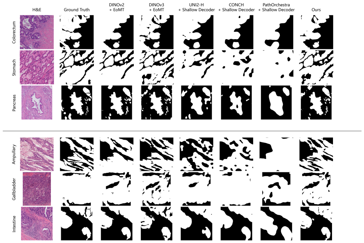
To complement the quantitative results, Figure 2 presents segmentation examples from all six organ domains. Across both seen and unseen cases, the proposed method generally follows the annotated tumor regions more closely and preserves irregular glandular structures and fragmented tumor boundaries. The comparison also illustrates the considerable morphological variation among organs, particularly in the unseen ampullary and gallbladder domains.

5. Discussion

The proposed method showed the best aggregate performance on both seen and unseen organs. Although its performance decreased from the seen group to the unseen group, it retained strong source-domain performance and achieved the highest pooled result on the unseen organs. This result suggests that pathology evidence can support cross-organ transfer without sacrificing segmentation performance on the source organs.

The per-domain results showed heterogeneous behavior across unseen target organs. Ampullary was consistently challenging across all compared methods. The proposed method achieved the highest score on this organ, suggesting that structured pathology evidence may help when the morphological difference between source and target organs is particularly large. This pattern may be related to the mixed histological features of ampullary adenocarcinoma, which can show intestinal, pancreatobiliary, and hybrid differentiation with variable local morphology [38]. T3s and DINOv2 with EoMT performed best on gallbladder and intestine, respectively; however, their advantages were specific to individual target organs. These differences show that the benefit of pathology evidence varies with organ-specific morphology and does not lead to uniform improvement across all target organs. Although our method did not achieve the highest score on every unseen organ, it showed the most consistent overall performance across the target set. This stability is clinically relevant because deployed systems are expected to remain reliable across specimens from different anatomical sites.

The comparison with foundation model-based methods further suggests that pretrained representations alone are not sufficient for robust dense segmentation under organ-level domain shift. Pathology foundation models are primarily pretrained as image encoders, and a task-specific segmentation head is needed to adapt their representations to pixel-level tumor prediction. With this adaptation, several foundation model-based systems achieved strong results on individual organs, showing that pretrained pathology features can transfer effectively to certain domains; however, this advantage was not consistent across all unseen organs, and their pooled unseen-domain performance remained lower than that of the proposed method. These results indicate that while pathology pretraining and task-specific decoding can provide useful representations, they do not by themselves ensure stable generalization to unseen organ morphology. In the selected examples shown in Figure 2, the proposed method more closely preserved small fragmented tumor regions, narrow internal gaps, and irregular boundary contours, while several foundation model-based systems produced smoother masks or omitted fine structures.

Among the domain generalization methods, both DCAC and T3s performed well on gallbladder. DCAC adapts its convolutional filters to domain and image content [34], whereas T3s aligns test-image style with the learned source-domain style space [4]. These mechanisms may be useful for gallbladder images, where recognizable glandular and stromal structures coexist with substantial variation in staining, inflammation, and fibrosis. However, neither method maintained this advantage on ampullary adenocarcinoma or in the pooled unseen-domain evaluation, for which the proposed method achieved higher performance.

Several limitations should be noted. The evaluation was conducted on patch-level images from the COSAS cohort using one prespecified training run. Repeated runs could provide a fuller assessment of sensitivity to model initialization. The evidence bank was generated and filtered through a fixed LLM-assisted procedure, and further review by pathologists could strengthen its clinical reliability. Evaluation on a single curated cohort may not fully reflect variations across institutions or the broader tissue context and slide-level artifacts encountered in whole-slide images. Future work will extend the evaluation to external multi-center datasets and WSI-level analysis. Fragmented tumor regions and poorly defined tumor–stroma boundaries also remained challenging in some cases.

6. Conclusions

This study investigated cross-organ adenocarcinoma segmentation in a source-only domain generalization setting and proposed an evidence-guided segmentation framework. The proposed method achieved the highest average performance on seen, unseen, and overall evaluation sets among the compared methods. These findings indicate the potential of structured morphological evidence to improve segmentation across unseen organs. Future work will focus on expert validation of the evidence bank and further evaluation using external multi-center datasets and whole-slide images.

References

1. Da, Q.; Wang, C.; Zuo, Y.; Guo, Y.; Jiang, G.; Shen, L.; Luo, X.; Ding, M.; Liu, J.; Hou, X.; et al. Cross-Organ and Cross-Scanner Adenocarcinoma Segmentation Challenge; Zenodo: Geneva, Switzerland, 2024. [Google Scholar] [CrossRef]
2. Zhou, K.; Liu, Z.; Qiao, Y.; Xiang, T.; Loy, C.C. Domain generalization: A survey. IEEE Trans. Pattern Anal. Mach. Intell. 2022, 45, 4396–4415. [Google Scholar] [CrossRef] [Scilit] [PubMed]
3. Jahanifar, M.; Raza, M.; Xu, K.; Vuong, T.T.L.; Jewsbury, R.; Shephard, A.; Zamanitajeddin, N.; Kwak, J.T.; Raza, S.E.A.; Minhas, F.; et al. Domain generalization in computational pathology: Survey and guidelines. ACM Comput. Surv. 2025, 57, 285. [Google Scholar] [CrossRef] [Scilit]
4. Meng, B.; Long, X.; Yang, W.; Liu, R.; Tian, Y.; Zheng, Y.; Liu, J. Advancing cross-organ domain generalization with test-time style transfer and diversity enhancement. In Proceedings of the 2025 IEEE 22nd International Symposium on Biomedical Imaging (ISBI), Houston, TX, USA, 14–17 April 2025; pp. 1–5. [Google Scholar]
5. Chen, R.J.; Ding, T.; Lu, M.Y.; Williamson, D.F.; Jaume, G.; Song, A.H.; Chen, B.; Zhang, A.; Shao, D.; Shaban, M.; et al. Towards a general-purpose foundation model for computational pathology. Nat. Med. 2024, 30, 850–862. [Google Scholar] [CrossRef] [Scilit] [PubMed]
6. Huang, Z.; Bianchi, F.; Yuksekgonul, M.; Montine, T.J.; Zou, J. A visual–language foundation model for pathology image analysis using medical twitter. Nat. Med. 2023, 29, 2307–2316. [Google Scholar] [CrossRef] [Scilit] [PubMed]
7. Lu, M.Y.; Chen, B.; Williamson, D.F.; Chen, R.J.; Liang, I.; Ding, T.; Jaume, G.; Odintsov, I.; Le, L.P.; Gerber, G.; et al. A visual-language foundation model for computational pathology. Nat. Med. 2024, 30, 863–874. [Google Scholar] [CrossRef] [Scilit] [PubMed]
8. Tellez, D.; Litjens, G.; Bándi, P.; Bulten, W.; Bokhorst, J.M.; Ciompi, F.; Van Der Laak, J. Quantifying the effects of data augmentation and stain color normalization in convolutional neural networks for computational pathology. Med. Image Anal. 2019, 58, 101544. [Google Scholar] [CrossRef] [Scilit] [PubMed]
9. Hoque, M.Z.; Keskinarkaus, A.; Nyberg, P.; Seppänen, T. Stain normalization methods for histopathology image analysis: A comprehensive review and experimental comparison. Inf. Fusion 2024, 102, 101997. [Google Scholar] [CrossRef] [Scilit]
10. Faryna, K.; van der Laak, J.; Litjens, G. Automatic data augmentation to improve generalization of deep learning in H&E stained histopathology. Comput. Biol. Med. 2024, 170, 108018. [Google Scholar] [CrossRef] [Scilit] [PubMed]
11. Nguyen, T.H.; Juyal, D.; Li, J.; Prakash, A.; Nofallah, S.; Shah, C.; Gullapally, S.C.; Yu, L.; Griffin, M.; Sampat, A.; et al. ContriMix: Scalable stain color augmentation for domain generalization without domain labels in digital pathology. In Proceedings of the MICCAI Workshop on Computational Pathology, Marrakesh, Morocco, 6–10 October 2024; Ciompi, F., Khalili, N., Studer, L., Poceviciute, M., Khan, A., Veta, M., Jiao, Y., Haj-Hosseini, N., Chen, H., Raza, S., et al., Eds.; Proceedings of Machine Learning Research: Cambridge, MA, USA, 2024; Volume 254, pp. 121–130. [Google Scholar]
12. Konwer, A.; Prasanna, P. MetaStain: Stain-Generalizable Meta-learning for Cell Segmentation and Classification with Limited Exemplars. In Proceedings of the International Conference on Medical Image Computing and Computer-Assisted Intervention, Marrakesh, Morocco, 6–10 October 2024; Springer: Berlin/Heidelberg, Germany, 2024; pp. 307–317. [Google Scholar]
13. Aubreville, M.; Stathonikos, N.; Bertram, C.A.; Klopfleisch, R.; Ter Hoeve, N.; Ciompi, F.; Wilm, F.; Marzahl, C.; Donovan, T.A.; Maier, A.; et al. Mitosis domain generalization in histopathology images—The MIDOG challenge. Med. Image Anal. 2023, 84, 102699. [Google Scholar] [CrossRef] [Scilit] [PubMed]
14. Aubreville, M.; Stathonikos, N.; Donovan, T.A.; Klopfleisch, R.; Ammeling, J.; Ganz, J.; Wilm, F.; Veta, M.; Jabari, S.; Eckstein, M.; et al. Domain generalization across tumor types, laboratories, and species—Insights from the 2022 edition of the mitosis domain generalization challenge. Med. Image Anal. 2024, 94, 103155. [Google Scholar] [CrossRef] [Scilit] [PubMed]
15. Xu, H.; Usuyama, N.; Bagga, J.; Zhang, S.; Rao, R.; Naumann, T.; Wong, C.; Gero, Z.; González, J.; Gu, Y.; et al. A whole-slide foundation model for digital pathology from real-world data. Nature 2024, 630, 181–188. [Google Scholar] [CrossRef] [Scilit] [PubMed]
16. Meng, B.; Yang, W.; Long, X.; Wang, Y.; Dang, K.; Zheng, Y.; Liu, J. PathVLG: A Vision-Language Framework for Domain Generalization in Cross-Organ Adenocarcinoma Segmentation. In Proceedings of the 2025 IEEE International Conference on Bioinformatics and Biomedicine (BIBM), Wuhan, China, 15–18 December 2025; pp. 5478–5485. [Google Scholar]
17. Zhou, K.; Yang, J.; Loy, C.C.; Liu, Z. Learning to prompt for vision-language models. Int. J. Comput. Vis. 2022, 130, 2337–2348. [Google Scholar] [CrossRef] [Scilit]
18. Menon, S.; Vondrick, C. Visual classification via description from large language models. arXiv 2022, arXiv:2210.07183. [Google Scholar]
19. Pratt, S.; Covert, I.; Liu, R.; Farhadi, A. What does a platypus look like? Generating customized prompts for zero-shot image classification. In Proceedings of the IEEE/CVF International Conference on Computer Vision, Paris, France, 1–6 October 2023; pp. 15691–15701. [Google Scholar]
20. Da, L.; Wang, R.; Xu, X.; Bhatia, P.; Kass-Hout, T.; Wei, H.; Xiao, C. FlanS: A Foundation Model for Free-Form Language-based Segmentation in Medical Images. In Proceedings of the 31st ACM SIGKDD Conference on Knowledge Discovery and Data Mining, Toronto, ON, Canada, 3–7 August 2025; pp. 404–414. [Google Scholar]
21. Zhao, Z.; Zhang, Y.; Wu, C.; Zhang, X.; Zhou, X.; Zhang, Y.; Wang, Y.; Xie, W. Large-vocabulary segmentation for medical images with text prompts. npj Digit. Med. 2025, 8, 566. [Google Scholar] [CrossRef] [Scilit] [PubMed]
22. Zhou, K.; Yang, Y.; Hospedales, T.; Xiang, T. Learning to generate novel domains for domain generalization. In Proceedings of the European Conference on Computer Vision, Virtual, 23–28 August 2020; Springer: Berlin/Heidelberg, Germany, 2020; pp. 561–578. [Google Scholar]
23. Zhou, K.; Yang, Y.; Qiao, Y.; Xiang, T. Domain generalization with mixstyle. arXiv 2021, arXiv:2104.02008. [Google Scholar]
24. Yang, Y.; Soatto, S. Fda: Fourier domain adaptation for semantic segmentation. In Proceedings of the IEEE/CVF Conference on Computer Vision and Pattern Recognition, Virtual, 13–19 June 2020; pp. 4085–4095. [Google Scholar]
25. Cheng, B.; Misra, I.; Schwing, A.G.; Kirillov, A.; Girdhar, R. Masked-attention mask transformer for universal image segmentation. In Proceedings of the IEEE/CVF Conference on Computer Vision and Pattern Recognition, New Orleans, LA, USA, 18–24 June 2022; pp. 1290–1299. [Google Scholar]
26. Yan, F.; Wu, J.; Li, J.; Wang, W.; Chen, Y.; Wei, L.; Lu, J.; Chen, W.; Gao, Z.; Li, J.; et al. Pathorchestra: A comprehensive foundation model for computational pathology with over 100 diverse clinical-grade tasks. npj Digit. Med. 2025, 8, 695. [Google Scholar] [CrossRef] [Scilit] [PubMed]
27. Kerssies, T.; Cavagnero, N.; Hermans, A.; Norouzi, N.; Averta, G.; Leibe, B.; Dubbelman, G.; De Geus, D. Your vit is secretly an image segmentation model. In Proceedings of the 2025 IEEE/CVF Conference on Computer Vision and Pattern Recognition (CVPR), Nashville, TN, USA, 11–15 June 2025; pp. 25303–25313. [Google Scholar]
28. Ranftl, R.; Bochkovskiy, A.; Koltun, V. Vision transformers for dense prediction. In Proceedings of the 2021 IEEE/CVF International Conference on Computer Vision (ICCV), Virtual, 11–17 October 2021; pp. 12159–12168. [Google Scholar]
29. Taha, A.A.; Hanbury, A. Metrics for evaluating 3D medical image segmentation: Analysis, selection, and tool. BMC Med. Imaging 2015, 15, 29. [Google Scholar] [CrossRef] [Scilit] [PubMed]
30. Ronneberger, O.; Fischer, P.; Brox, T. U-net: Convolutional networks for biomedical image segmentation. In Proceedings of the International Conference on Medical Image Computing and Computer-Assisted Intervention, Munich, Germany, 5–9 October 2015; Springer: Berlin/Heidelberg, Germany, 2015; pp. 234–241. [Google Scholar]
31. Zhou, Z.; Rahman Siddiquee, M.M.; Tajbakhsh, N.; Liang, J. Unet++: A nested u-net architecture for medical image segmentation. In Proceedings of the International Workshop on Deep Learning in Medical Image Analysis, Granada, Spain, 20 September 2018; Springer: Berlin/Heidelberg, Germany, 2018; pp. 3–11. [Google Scholar]
32. Cao, H.; Wang, Y.; Chen, J.; Jiang, D.; Zhang, X.; Tian, Q.; Wang, M. Swin-unet: Unet-like pure transformer for medical image segmentation. In Proceedings of the European Conference on Computer Vision, Tel Aviv, Israel, 23–27 October 2022; Springer: Berlin/Heidelberg, Germany, 2022; pp. 205–218. [Google Scholar]
33. Benigmim, Y.; Roy, S.; Essid, S.; Kalogeiton, V.; Lathuilière, S. Collaborating foundation models for domain generalized semantic segmentation. In Proceedings of the IEEE/CVF Conference on Computer Vision and Pattern Recognition, Seattle, WA, USA, 16–22 June 2024; pp. 3108–3119. [Google Scholar]
34. Hu, S.; Liao, Z.; Zhang, J.; Xia, Y. Domain and content adaptive convolution based multi-source domain generalization for medical image segmentation. IEEE Trans. Med. Imaging 2022, 42, 233–244. [Google Scholar] [CrossRef] [Scilit] [PubMed]
35. Zhou, Q.; Zhang, K.Y.; Yao, T.; Lu, X.; Ding, S.; Ma, L. Test-time domain generalization for face anti-spoofing. In Proceedings of the IEEE/CVF Conference on Computer Vision and Pattern Recognition, Seattle, WA, USA, 16–22 June 2024; pp. 175–187. [Google Scholar]
36. Oquab, M.; Darcet, T.; Moutakanni, T.; Vo, H.; Szafraniec, M.; Khalidov, V.; Fernandez, P.; Haziza, D.; Massa, F.; El-Nouby, A.; et al. Dinov2: Learning robust visual features without supervision. arXiv 2023, arXiv:2304.07193. [Google Scholar]
37. Siméoni, O.; Vo, H.V.; Seitzer, M.; Baldassarre, F.; Oquab, M.; Jose, C.; Khalidov, V.; Szafraniec, M.; Yi, S.; Ramamonjisoa, M.; et al. Dinov3. arXiv 2025, arXiv:2508.10104. [Google Scholar]
38. Reid, M.D.; Balci, S.; Ohike, N.; Xue, Y.; Kim, G.E.; Tajiri, T.; Memis, B.; Coban, I.; Dolgun, A.; Krasinskas, A.M.; et al. Ampullary carcinoma is often of mixed or hybrid histologic type: An analysis of reproducibility and clinical relevance of classification as pancreatobiliary versus intestinal in 232 cases. Mod. Pathol. 2016, 29, 1575–1585. [Google Scholar] [CrossRef] [Scilit] [PubMed]
Figure 1. Overview of the proposed evidence-guided segmentation framework. The solid blue pathway is used during both training and inference. The CONCH image encoder extracts multi-level visual features, the Semantic Query Booster (SQB) forms image-aware queries using class-domain text embeddings, and positive pathology evidence recalibrates these queries before mask decoding. The evidence bank is constructed offline from source-domain training data, while positive and negative evidence jointly provide matched-evidence supervision during training. The green dashed pathway denotes the training-only text-conditioned feature–style generation branch. During inference, the feature–style branch and all loss computations are removed, with only the image encoder, fixed text embeddings, SQB, evidence-guided query recalibration, and mask decoder retained.
Electronics 15 03691 g001
Figure 2. Qualitative comparison across the six organ domains. The upper panel presents the seen domains of colorectum, stomach, and pancreas, while the lower panel presents the unseen domains of ampullary, gallbladder, and intestine. From left to right, each row shows the H&E image, ground truth mask, and predictions produced by DINOv2 with EoMT, DINOv3 with EoMT, UNI2-h with a shallow decoder, CONCH with a shallow decoder, PathOrchestra with a shallow decoder, and the proposed method. Within each organ, the displayed case was selected as the non-empty test sample in which the foreground IoU for the proposed method was closest to the organ-specific median.
Electronics 15 03691 g002