Valley-Polarized Transport in Graphene Induced by Asymmetric Strain and Ferromagnetic Modulation

Abstract

In this work, we theoretically investigate the valley-dependent electron transport properties of graphene modulated by two strained regions and a single ferromagnetic stripe based on the Dirac equation and the transfer-matrix method. By constructing a multi-region model, the conductances of the K and K’ valleys as well as the corresponding valley polarization are systematically calculated. The effects of the magnetic vector-potential, the strain-induced gauge potentials, the widths of the strained regions, and the competition parameter $\lambda$ on the valley-resolved transport behavior are analyzed in detail. The results show that both the conductance and the valley polarization are highly sensitive to the external modulation parameters and the geometric structural parameters. By properly tuning the relative strength and spatial distribution of the magnetic vector-potential and strain, an effective control of valley polarization can be achieved. This work deepens the understanding of valley-dependent transport mechanisms in graphene and provides theoretical guidance for tunable valley filtering in graphene-based systems.

1. Introduction

Graphene is a two-dimensional Dirac material possessing two inequivalent valleys at the corners of the Brillouin zone, labeled K and K’. These valley degrees of freedom provide an additional quantum number for charge carriers, giving rise to the emerging field of valleytronics, which aims to encode, manipulate, and detect information using the valley index [1,2]. Similar to spin polarization in spintronics, valley polarization refers to an imbalance in carrier populations between the K and K’ valleys and plays a central role in valley-based functional devices. Therefore, achieving stable and controllable valley polarization has become an important scientific issue in the development of next-generation electronic and information-processing technologies [3,4,5,6,7,8,9]. In recent years, research on valley-dependent transport in graphene and related two-dimensional materials has attracted increasing attention [10,11,12,13,14]. Previous theoretical studies have shown that magnetic barriers, electric potentials, Dirac gaps, and strain-induced pseudomagnetic fields can reshape graphene transport spectra and generate wave-vector or valley-selective effects [15,16,17,18]. Meanwhile, graphene-based device studies, including graphene nanoribbons and graphene/h-BN tunneling heterostructures, have demonstrated the feasibility of engineering spin- and tunneling-related transport properties through structural design [19,20].These studies indicate that combining external modulation with structural engineering provides an effective route for controlling valley-dependent transport in graphene.

At present, an increasing number of studies have focused on valley-dependent electronic transport in graphene and related two-dimensional materials, where various external modulation schemes have been proposed to generate and control valley polarization [21,22,23,24,25]. Rycerz et al. theoretically demonstrated that a graphene quantum point contact with zigzag edges can act as an efficient valley filter by exploiting the intrinsic valley-selective boundary states [26]. Guinea et al. further revealed that nonuniform mechanical strain can produce extremely large pseudomagnetic fields in graphene, providing a powerful route to engineer valley-dependent gauge potentials [27], which was experimentally confirmed by Levy et al. through the observation of strain-induced Landau levels corresponding to pseudomagnetic fields exceeding 300 T [28]. Anna and Martino analyzed transport through magnetic barriers in graphene and demonstrated that magnetic vector potentials can strongly reshape transmission spectra and induce valley-selective effects [29]. Moreover, the combination of ferromagnetic stripes and strain has been proposed as a viable strategy for tunable valley polarization [30,31,32]. Beyond monolayer graphene, Gorbachev et al. experimentally observed the valley Hall effect in gapped graphene systems, providing direct evidence of valley-contrasting transport under broken inversion symmetry [33]. Similar valley Hall phenomena have been reported in transition metal dichalcogenides [1]. The above research indicates that artificially engineered heterostructures and patterned magnetic field configurations can further enhance the controllability of valley polarization and provide useful guidance for designing valley-selective graphene structures.

Most existing studies focus on either strain-induced pseudomagnetic fields or magnetic modulation separately, while the cooperative and competitive interplay between asymmetric strain fields and ferromagnetic vector potentials has not been systematically investigated. In particular, the majority of previous works consider symmetric configurations or single-barrier structures, where the valley polarization is mainly attributed to a single source of symmetry breaking. Different from single-barrier or symmetric magnetic-strain structures, the present model contains two separated strain regions and one central ferromagnetic stripe. The two strain regions can have different strengths and widths. Their spatial separation introduces additional phase accumulation between the strain and magnetic modulations. As a result, the valley-dependent transmission can be tuned by strain asymmetry, magnetic modulation, and their relative arrangement. However, in realistic structures, spatial asymmetry and multi-region modulation are inevitable, and the interaction between strain and magnetic barriers makes valley transport both more complex and more tunable. Therefore, it is necessary to construct a comprehensive model that incorporates asymmetric strain regions and ferromagnetic modulation in order to deeply understand its transport mechanism and provide new theoretical basis for achieving controllable valley polarization.

We investigate valley-polarized transport in graphene induced by asymmetric strain and ferromagnetic modulation within a unified theoretical framework. By introducing two strain regions with different strengths together with a ferromagnetic stripe, we establish a multi-region model based on the Dirac equation and employ the transfer-matrix method to calculate the valley-resolved transmission coefficients and conductances. We systematically analyze the effects of strain asymmetry, magnetic vector-potential, and structural parameters on the evolution of conductance in the K and K’ valleys, as well as on the resulting valley polarization. Our results demonstrate that effective control of valley polarization can be achieved within appropriate parameter regimes, providing additional degrees of freedom and theoretical guidance for tunable valley-filtering structures.

2. Theoretical Method

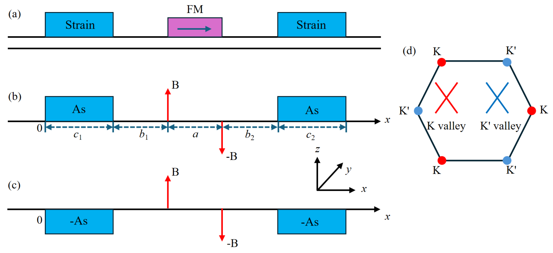
In this work, we consider a graphene-based heterostructure consisting of two strain regions and a ferromagnetic stripe, as illustrated in Figure 1a. The system is divided into seven regions along the transport direction x: a free region, a strain region with strength, a spacer region, a ferromagnetic (FM) stripe, another spacer region, a second strain region with strength, and finally a free outgoing region.

The geometric parameters of the structure are schematically shown in Figure 1b. The widths of the two strain regions are denoted by $c_1$ and $c_2$, respectively. The FM stripe width is a. The widths of two spacer regions separating the strain and magnetic regions are $b_1$ and $b_2$. Figure 1b,c further illustrate the effective vector potential fields for electrons near the two valleys K and K’. The strain regions generate valley-dependent gauge potentials, whereas the FM stripe introduces a magnetic vector-potential that modifies the transverse momentum of carriers. Such a multi-region structure allows us to investigate the interplay between asymmetric strain modulation and ferromagnetic magnetic barriers on valley-dependent transport. A possible implementation route is to fabricate a graphene channel on a patterned or flexible substrate to form local strain regions and deposit a narrow ferromagnetic stripe above the channel to provide magnetic modulation. The spacer regions in the model correspond to the unstrained graphene sections between the strained regions and the ferromagnetic stripe. Therefore, the low-energy electronic properties of graphene can be described by the Dirac Hamiltonian,

$$H_{\eta }=v_F\sigma ·\left(\mathbf{p}+{\mathbf{A}}_{\eta }\right)$$

(1)

where $v_F$ is the Fermi velocity in graphene, $\sigma =({\sigma }_x,{\sigma }_y)$ represent the Pauli matrices, and $\mathbf{p}=(p_x,p_y)$ is the momentum operator. In this normalized form, the electron charge and ℏ are absorbed into the effective vector potential ${\mathbf{A}}_{\eta }$, and the valley index is defined as $\eta =+1$ for the K valley and $\eta =-1$ for the K’ valley. The present work is based on the low-energy continuum Dirac model, where the strain and magnetic modulations are described by effective gauge potentials. Such a framework is suitable for analyzing ballistic valley-dependent transport and has been widely used in graphene magnetic-barrier and strain-engineering studies. The effective vector potential ${\mathbf{A}}_{\eta }$ that the electron experiences in this structure consists of two contributions, the strain-induced gauge vector potential and the magnetic vector-potential generated by the FM stripe. In strained graphene, the gauge potential is valley dependent and takes opposite signs for the two inequivalent valleys, which can be written as $A_s\left(x\right)=\eta A_s$, where $\eta =\pm 1$ corresponds to the K and K’ valleys. The strain-induced gauge potential comes from strain-modified nearest-neighbor hopping in graphene. Its value depends on the strain tensor and the crystallographic orientation. In this effective model, $A_{s1}$ and $A_{s2}$ denote dimensionless gauge-potential strengths of two local uniaxial strain regions. The scalar deformation potential is not included because it is valley independent. In the Landau gauge, the vector potential can be expressed as ${\mathbf{A}}_{\eta }\left(x\right)=[0,A\left(x\right),0]$, $A\left(x\right)$ varies along the transport direction x. Therefore, the total effective vector potential in different regions can be written in a piecewise form as

$$A\left(x\right)=\left\{\begin{array}{cc}0\hfill & x<0\hfill \\ \eta A_{s1}\hfill & 0<x<c_1\hfill \\ 0\hfill & c_1<x<c_1+b_1\hfill \\ B\hfill & c_1+b_1<x<c_1+b_1+a\hfill \\ 0\hfill & c_1+b_1+a<x<c_1+b_1+a+b_2\hfill \\ \eta A_{s2}\hfill & c_1+b_1+a+b_2<x<c_1+b_1+a+b_2+c_2\hfill \\ 0\hfill & x>c_1+b_1+a+b_2+c_2\hfill \end{array}\right..$$

(2)

Here, $A_{s1}$ and $A_{s2}$ denote the strain-induced gauge potentials in the two strained regions, while the symbol B denotes the magnetic vector-potential generated by the FM stripe. In the Landau gauge, the corresponding magnetic field is related to the vector potential by $B_z\left(x\right)=\partial A_y\left(x\right)/\partial x$.

For convenience in numerical calculations, all physical quantities in this work are expressed in dimensionless units with $E\to E_{0}E,B\left(x\right)\to B_{0}B\left(x\right),\mathrm{r}\to l_0\mathrm{r},k\to k/l_0$, and ${\mathrm{A}}_s\left(x\right)\to B_0{l}_0{\mathrm{A}}_s\left(x\right)$. The energy is scaled by the characteristic energy $E_0=\hslash v_F/l_0$, where $l_0$ is a characteristic length of the system. For $B_0$ = 0.1 T, $l_0$ = 81.1 nm, $E_0$ = 7.0 meV. To make the dimensionless parameters clearer, the main parameters used in the numerical calculations and their physical conversions are summarized in

Table 1. Normalization relations between the dimensionless parameters and physical scales.

Quantity	Dimensionless Parameter	Physical Conversion
Energy	E	$E_{\mathrm{phys}}=E{E}_0$, $E_0=7.0$ meV
Length	L	$L_{\mathrm{phys}}=L{l}_0$, $l_0=81.1$ nm
Magnetic field scale	B	$B_{\mathrm{phys}}=B{B}_0$, $B_0=0.1$ T
Strain-induced gauge potential	$A_s$	$A_{s,\mathrm{phys}}=A_s{B}_0{l}_0$
FM stripe width	$a=1.0$	$a_{\mathrm{phys}}=81.1$ nm
Spacer widths	$b_1=b_2=1.0$	$b_{1,\mathrm{phys}}=b_{2,\mathrm{phys}}=81.1$ nm
Strain-region widths	$c_1=c_2=1.0$	$c_{1,\mathrm{phys}}=c_{2,\mathrm{phys}}=81.1$ nm

. Under this normalization, $A_{s1}$, $A_{s2}$, and B are expressed in the same dimensionless units and can be used consistently in Equations (1) and (2).

Because the system is translationally invariant along the y direction, the transverse momentum $k_y$ is conserved during the transport. Therefore, the electron wave function in each region is as follows:

$${\mathrm{\Psi }}_j(x,y)={\psi }_j{e}^{i{k}_{y}y}.$$

(3)

Substituting this expression into the Dirac equation, the longitudinal wave vector in the j-th region is obtained as $q_j=\sqrt{E^2-{(k_y+A_j)}^2}$, where E is the incident energy and $A_j$ represents the effective vector potential in region j. When $E^2-{(k_y+A_j)}^2<0$, the longitudinal wave vector $q_j$ becomes complex and the corresponding mode is evanescent. In the calculation, the square-root branch is chosen with $\mathrm{Im}\left(q_j\right)\ge 0$. The complex value of $q_j$ is kept in the spinor basis and in the transfer matrix. The low-energy resonances were checked by refining the energy and incident-angle grids and by verifying probability conservation. The electron wave function can be expressed as a superposition of forward and backward propagating states

$${\psi }_j\left(x\right)=a_j\left(\begin{array}{c}1\\ {\displaystyle \frac{q_j+i(k_y+A_j)}{E}}\end{array}\right)e^{i{q}_{j}x}+b_j\left(\begin{array}{c}1\\ {\displaystyle \frac{-q_j+i(k_y+A_j)}{E}}\end{array}\right)e^{-i{q}_{j}x},$$

(4)

where $a_j$ and $b_j$ are the coefficients of the forward and backward waves, respectively. For clarity, the wave function in the j-th region can be written as ${\psi }_j\left(x\right)=W_j\left(x\right)C_j$, where $C_j={(a_j,b_j)}^T$ and $W_j\left(x\right)$ is constructed from the two spinor basis functions in Equation (4). At an interface $x=x_j$, the continuity condition gives $C_j=W_j^{-1}\left(x_j\right)W_{j+1}\left(x_j\right)C_{j+1}$. The total transfer matrix is then obtained as $M={\prod }_{j=1}^6{W}_j^{-1}\left(x_j\right)W_{j+1}\left(x_j\right)$, where the interface positions are $x_j=0,c_1,c_1+b_1,c_1+b_1+a,c_1+b_1+a+b_2,c_1+b_1+a+b_2+c_2$. The incident, reflected, and transmitted amplitudes are related by

$$\left({\displaystyle \genfrac{}{}{0pt}{}{1}{r}}\right)=M\left({\displaystyle \genfrac{}{}{0pt}{}{t}{0}}\right),$$

(5)

where r and t denote the reflection and transmission amplitudes, respectively. From the transfer matrix, the electron transmission probability can be calculated from the following formula,

$$T_{\eta }(E,k_y)={\displaystyle \frac{q_7}{q_1}}\left|t^2\right|.$$

(6)

This expression follows from the ratio of the transmitted and incident longitudinal probability currents. In the present structure, the incident and outgoing regions are identical, so $q_7/q_1=1$. In the numerical calculation, the reflection probability is defined as $R_{\eta }={\left|r\right|}^2$, and the probability conservation condition $R_{\eta }+T_{\eta }=1$ is checked. The implementation was also tested in the single-barrier and symmetric-barrier limits. To evaluate the transport properties, the valley-resolved conductance is calculated using the Landauer-Büttiker formalism. After integrating over all possible incident angles, the conductance is given by

$$G_{\eta }\left(E\right)=G_0{\int }_{-\pi /2}^{\pi /2}{T}_{\eta }(E,\varphi )cos\varphi d\varphi .$$

(7)

Here, $T_{\eta }(E,\varphi )$ is the transmission probability for electrons with energy E and incident angle $\varphi$. The factor $cos\varphi$ is the projection of the carrier velocity along the transport direction. The normalization factor $G_0=2e^{2}E{L}_y/\left(\pi h\right)$ is used for one valley, where the factor 2 accounts for spin degeneracy, E is the dimensionless incident energy, and $L_y$ is the transverse width of the graphene channel. Finally, the valley polarization is defined as

$$P\left(E\right)={\displaystyle \frac{G_K-G_{K^{\prime }}}{G_K+G_{K^{\prime }}}}.$$

(8)

3. Results and Discussion

In this section, the valley-dependent electronic transport properties of the proposed structure are numerically investigated based on the theoretical model. Unless otherwise specified, the geometric parameters of the structure are fixed as follows: the width of the ferromagnetic stripe is $a=1.0$, the free region between Strain-1 and the FM stripe is $b_1=1.0$, and the free region between the FM stripe and Strain-2 is $b_2=1.0$. The effects of the magnetic vector-potential, the widths of the strained regions, and the strain-induced gauge potentials on the conductance and valley polarization are systematically analyzed. The chosen parameters are used as effective modulation strengths to reveal the general transport trends rather than to describe one specific fabricated sample.

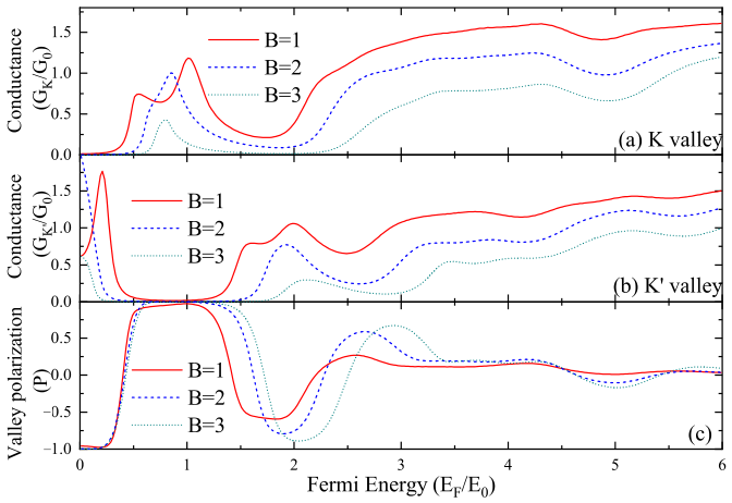
The influence of the magnetic vector-potential B on the electron conductance and corresponding valley polarization of the system is shown in Figure 2. The widths of two strained regions are taken as $c_1=1.0$ and $c_2=1.0$, while the strain-induced gauge potentials are fixed at $A_{s1}=1.0$ and $A_{s2}=1.0$.

The conductance spectra shown in Figure 2a,b exhibit pronounced differences under different values of the magnetic vector-potential, indicating that magnetic modulation plays a crucial role in regulating electron transport and valley polarization. In the high-energy regime, smaller magnetic vector-potential values cause the conductance curves to shift toward lower energies, whereas in the low-energy regime, larger B leads to more evident leftward shifts. The transition between these two regimes occurs around the Fermi energy $E_F/E_0=2$ for the K valley and around $E_F/E_0=1$ for the K’ valley, reflecting the valley-dependent response to magnetic modulation. In addition, the K’ valley exhibits a pronounced conductance peak in the very low-energy region close to the Dirac point, and this peak persists for all values of the magnetic vector-potential while gradually shifting toward lower energies with increasing B. This feature may be associated with resonant tunneling caused by multiple reflections between different gauge-potential regions. It is sensitive to the phase accumulation of low-energy carriers. Therefore, we describe it as a possible resonant feature. This valley contrast is caused by the opposite signs of the strain-induced gauge potential in the two valleys, which lead to different effective transverse-momentum matching conditions. For the K valley, the mismatch is enhanced and low-energy transmission is suppressed, whereas for the K’ valley the mismatch can be partially compensated, allowing finite resonant transmission near the Dirac point. The nonzero valley polarization originates from the combined breaking of valley equivalence. The strain-induced gauge potential has opposite signs in the K and K’ valleys. The magnetic vector-potential shifts the transverse momentum in the same direction for both valleys. When these two effects are combined with spatially asymmetric strain regions, the effective momentum matching becomes different for the two valleys. As a result, $G_K$ and $G_{K^{\prime }}$ become unequal. In limiting cases such as vanishing magnetic modulation or fully symmetric strain regions, this valley contrast is expected to be weakened. Reversing the magnetization changes the sign of the magnetic vector-potential and can reverse the preferred valley. The valley polarization presented in Figure 2c more directly reveals the regulatory effect of magnetic modulation. Overall, a stronger magnetic vector-potential produces higher valley polarization, demonstrating that magnetic barriers enhance valley selectivity. However, in the high-energy regime, the degree of valley polarization gradually decreases and approaches zero, indicating that high-energy carriers become less sensitive to magnetic confinement. By comparing the conductance and valley polarization spectra, it can be found that conductance reflects the overall transmission capability of carriers, whereas valley polarization characterizes the imbalance between the two valleys. As magnetic modulation strengthens, total transmission is suppressed while valley selectivity is enhanced, leading to opposite variation trends between conductance magnitude and polarization intensity. These results demonstrate that the magnetic vector-potential effectively regulates valley-resolved transport and provides theoretical insight into tunable valley filtering.

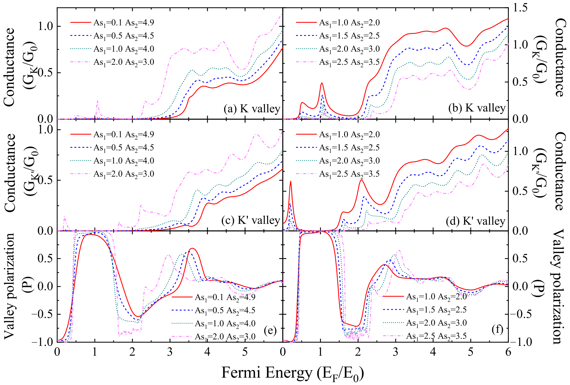
To investigate the influence of different strain strengths on the transport properties of the system, Figure 3 presents the conductance and valley polarization under different combinations of the strain-induced gauge potentials $A_{s1}$ and $A_{s2}$. In these calculations, the magnetic vector-potential is fixed at $B=1$, and the widths of the two strain regions are chosen as $c_1=1.0$ and $c_2=1.0$, respectively. Figure 3a,c,e show the results for the case where the sum of the strain-induced gauge potentials is kept constant, i.e., $A_{s1}+A_{s2}=5.0$. Figure 3b,d,f correspond to the case where the difference between the two strain potentials is fixed, i.e., $A_{s2}-A_{s1}=1.0$. From Figure 3a,c, it can be observed that when the total strain strength is fixed, the conductance spectra of both the K and K’ valleys gradually shift toward lower energies as $A_{s1}$ increases. Meanwhile, the conductance is enhanced with increasing $A_{s1}$, indicating that a more symmetric strain configuration leads to higher transmission. This behavior can be attributed to the reduction of effective scattering asymmetry and the improved matching of wave vectors between adjacent regions. The influence of strain asymmetry on valley polarization is more clearly demonstrated in Figure 3e, where the polarization reaches its maximum around $E\approx 1$ for different strain configurations. With increasing asymmetry, the energy range over which high polarization is maintained becomes broader, and the polarization peaks shift toward lower energies. This phenomenon can be explained by the enhanced valley-dependent phase accumulation induced by asymmetric gauge potentials. In contrast, Figure 3b,d show that when the difference between the two strain potentials is fixed, the conductance in both valleys decreases as $A_{s1}$ and $A_{s2}$ increase. This indicates that a stronger modulation will form a more effective barrier, and electron transmission will be suppressed as a result. Figure 3f further shows the corresponding valley polarization. It can be seen that a larger overall strain strength enhances the degree of valley polarization. This enhancement is more evident in the low-energy regime, where the polarization remains nearly unchanged at a high level. In the higher energy range, the polarization peaks shift toward higher energies and their magnitudes gradually increase. This can be attributed to the combined effect of stronger gauge fields and increased valley-dependent scattering. Overall, these results demonstrate that asymmetric strain plays a significant role in modulating both conductance and valley polarization, providing a useful theoretical route for tunable valley-selective transport.

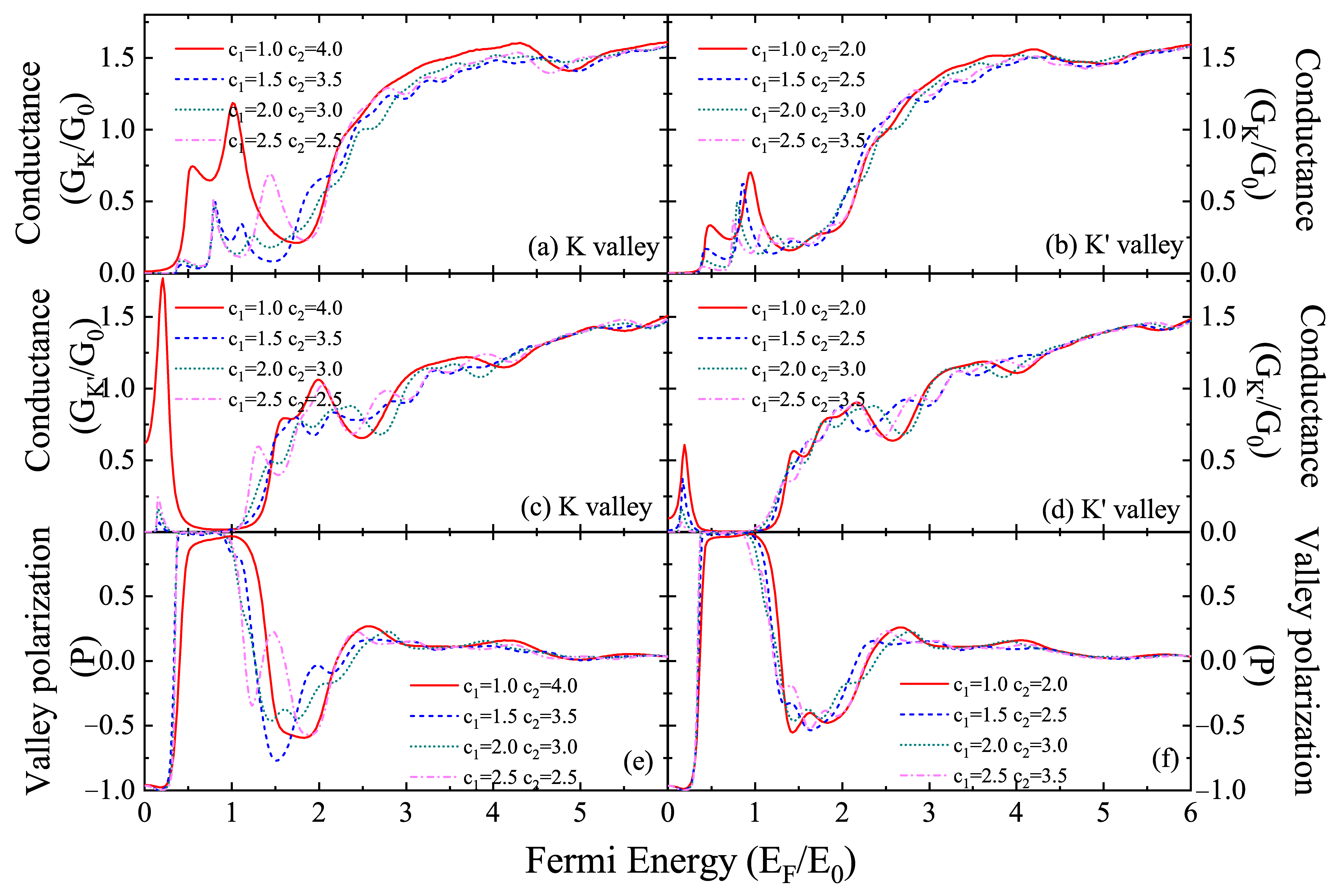
Figure 4 shows the conductance and the corresponding valley polarization for different widths of the two strained regions, while the strain-induced gauge potentials are fixed at $A_{s1}=A_{s2}=1.0$. Figure 4a,c,e correspond to the case where the total width of the two strained regions is constant, i.e., $c_1+c_2=5.0$, whereas Figure 4b,d,f show the results for a fixed width difference, i.e., $c_2-c_1=1.0$. From Figure 4a,c, it can be seen that when the total width of the two strain regions is fixed, changing the distribution of $c_1$ and $c_2$ mainly affects the resonant transport behavior of the low-energy and the intermediate energy regions. The conductance spectra of both valleys exhibit obvious differences in peak height and peak position, indicating that the redistribution of the two strained widths can effectively tune the wave-vector matching. As the Fermi energy increases, the differences between the various curves gradually decrease and tend to converge in the high-energy region. The corresponding valley polarization shown in Figure 4e further demonstrates that the width asymmetry of the strained regions has a strong influence on the polarization spectrum. On the other hand, Figure 4b,d show that when the width difference is fixed, simultaneously increasing $c_1$ and $c_2$ also changes the conductance spectra of the two valleys. Figure 4f presents the corresponding valley polarization curves, showing that the oscillations of the curves are still strongly affected by the absolute widths of the two strained regions. These results indicate that not only the strain strength but also the geometric widths of the strained regions can effectively modulate the conductance and valley polarization. In this work, the ferromagnetic stripe width a and the spacer widths $b_1$ and $b_2$ are kept fixed in order to isolate the main effects of asymmetric strain and magnetic modulation. Physically, changing a mainly modifies the effective interaction length of the magnetic barrier, while changing $b_1$ and $b_2$ changes the phase accumulation between different modulation regions and thus affects the resonance oscillations. Therefore, fixing these geometric parameters allows the primary strain- and magnetic-modulation effects on valley-resolved conductance and valley polarization to be identified more clearly.

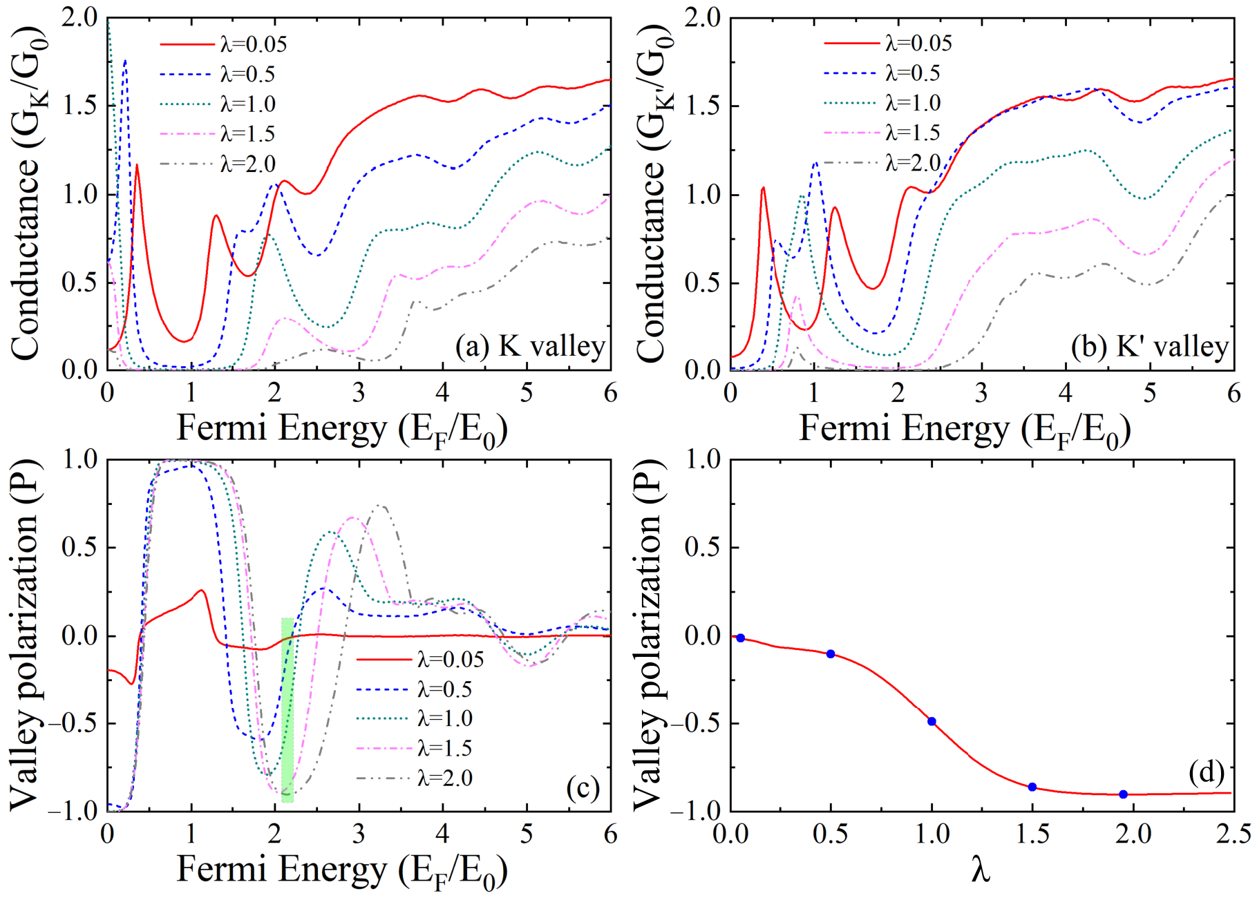
In order to further reveal the competition between magnetic modulation and strain modulation, Figure 5 introduces a competition parameter $\lambda =B/A_s$. Here, $\lambda$ measures the relative strength of magnetic modulation to strain-induced gauge modulation. It is used to distinguish the strain-dominated and magnetic-dominated transport regimes. In this part, the two strain potentials are kept equal, namely $A_{s1}=A_{s2}=A_s$, and the value of $\lambda$ is tuned by changing the magnetic vector-potential B. It should be noted that $\lambda$ is a relative parameter. It is not a unique scaling variable. The transport spectra still depend on the individual values of B and $A_s$. This is because both parameters enter the longitudinal wave vector and the phase accumulation in each region. Therefore, different pairs of $(B,A_s)$ with the same $\lambda$ generally do not give identical conductance or valley-polarization spectra. In Figure 5, $A_s$ is fixed and B is varied. Thus, the plotted results show the effect of increasing magnetic modulation relative to a fixed strain background. The separate effects of B and $A_s$ are discussed in Figure 2 and Figure 3. Figure 5a,b show the conductance of the K and K’ valleys as functions of the Fermi energy for different values of $\lambda$. Figure 5c gives the corresponding valley polarization. It can be seen from Figure 5a,b that the conductance of both the K and $K^{\prime }$ valleys decreases with increasing $\lambda$. When $\lambda$ is small, the system is mainly dominated by the strain modulation, and the overall conductance remains relatively high. As $\lambda$ gradually increases, the magnetic modulation becomes stronger, gradually suppressing the conductance. Figure 5c shows that the valley polarization exhibits significantly different evolution behaviors for different values of $\lambda$. When $\lambda$ is small, the valley polarization curve is relatively smooth. However, with increasing $\lambda$, stronger oscillations appear in a specific energy range, and the extrema become more pronounced. To illustrate this variation more clearly, a typical region is highlighted by the green shaded area in Figure 5c. The corresponding valley polarization in this shaded region is presented as a function of $\lambda$ in Figure 5d. It is found that, with increasing $\lambda$, the valley polarization first decreases slowly, then drops rapidly, and finally tends to become stable. This indicates that the evolution of valley polarization is not linear when the system gradually changes from the strain-dominated regime to the magnetic vector-potential-dominated regime. These results indicate that the competition parameter $\lambda$ can serve as an important physical quantity to describe the interplay between the magnetic vector-potential and the strain. It also provides a new way to realize controllable valley polarization through the combined tuning of magnetic vector-potential and strain.

The present structure is designed to reveal the combined effect of strain modulation, magnetic modulation, and spatial asymmetry. The separate influences of strain strength, strain-region width, and relative magnetic modulation are shown in Figure 3, Figure 4 and Figure 5. These comparisons indicate that the valley polarization arises from the combined action of these factors rather than from a single modulation alone.

From the viewpoint of device operation, the spectra in Figure 2, Figure 3, Figure 4 and Figure 5 can be further evaluated by several quantitative indicators. The first one is the maximum valley polarization, ${\left|P\right|}_{max}$, which characterizes the strongest valley-filtering capability achievable within the investigated energy range. The second one is the effective high-polarization energy window, $\Delta E_{\mathrm{HP}}$, defined as the continuous energy interval in which the absolute valley polarization remains above a selected threshold, $\left|P\right|>50\%$. The third one is the transmission efficiency, represented by $G_{\mathrm{tot}}=G_K+G_{K^{\prime }}$, while $G_{\mathrm{valley}}=|G_K-G_{K^{\prime }}|$ describes the transmitted valley imbalance. These indicators show that an optimal valleytronic operating regime should not be determined only by the peak value of P, because a very large polarization may occur together with a strongly suppressed conductance. Therefore, the practically useful parameter region corresponds to the energy interval where high valley polarization and non-negligible total conductance coexist. In the present structure, increasing the magnetic vector-potential or the competition parameter $\lambda$ generally enhances the valley selectivity, but also reduces the overall conductance. This reveals a trade-off between valley-filtering strength and transmission efficiency, which should be considered in future device optimization.

4. Conclusions

In this work, the valley-dependent electron transport properties of graphene modulated by two strained regions and a single ferromagnetic stripe have been investigated based on the Dirac equation and the transfer-matrix method. The influences of the magnetic vector-potential, the strain strength, the widths of the strained regions, and the competition parameter $\lambda$ on the valley-resolved conductance and valley polarization have been discussed in detail. The results show that strong valley polarization can be obtained in the low-energy region, especially around the resonant energy window near $E\sim 1$. In this region, the useful operating condition should be identified by considering both the valley polarization and the total conductance. For the representative structure used in the calculations, the fixed geometric parameters are a, $b_1$ and $b_2$. The strained-region widths are tunable through $c_1$ and $c_2$, and the results indicate that asymmetric strain distribution and increased magnetic modulation are favorable for enhancing valley selectivity. In particular, the introduction of the competition parameter $\lambda$ reveals a clear nonlinear competitive relation between magnetic modulation and strain modulation. The discussion of maximum valley polarization, effective high-polarization energy window, and total conductance further clarifies the device-relevant trade-off between polarization strength and transmission efficiency. It should also be noted that the present model is based on ideal ballistic transport. Finite-temperature broadening, disorder scattering, and contact effects are not included and should be considered in future device-level studies. These findings may provide useful theoretical guidance for the structural optimization of graphene-based valley-filtering systems.