PL-RiskPlanner: Safety-Constrained Risk-Aware Path Planning for UAV Inspection in Simulated Power-Line Corridors

Abstract

Path planning for power-line inspection requires asset-specific clearance from conductors, towers, and insulators, together with temporal separation from moving obstacles. Existing methods often optimize path length or a soft risk objective without showing that a single, explicit feasibility predicate is enforced during both search and postprocessing. We propose PL-RiskPlanner, a constraint-consistent framework that applies asset- and obstacle-specific checks before admitting grid edges, ranks the admitted edges using a power-line risk field, predicts moving-object positions at estimated UAV arrival times, and applies the same sampled verifier during smoothing. The contribution lies not in a new or faster A* search rule but in a power-line-specific feasible-set formulation that remains consistent across search, shortcutting, and final evaluation. A bounded margin accounts for uncertainty in velocity estimates. We evaluate eight executable planners across six synthetic scenario families and conduct controlled experiments on obstacle density, component ablation, risk weights, route crossings, prediction noise, and equal verifier budgets. Across 1800 nominal PL-RiskPlanner trials, no safety flag was recorded by the independent evaluator (Wilson 95% upper bound, 0.21%), and the mean verified-path length was 110.64 m. In controlled route crossings, the no-prediction variant produced 222 flags in 300 trials, whereas no safety flag was recorded for the complete planner. At velocity-noise level 0.4, the uncertainty margin changed the flag count from 203 to 47 and increased the mean simulator-reference dynamic clearance from −0.27 to 2.23 m. A 3600-trial equal-verifier-budget audit quantifies the resulting completion–computation trade-off without equating algorithm-specific iteration counters. Although the 50,400 trial records are specific to the stated simulator, they provide a reproducible protocol for safety-constrained inspection-path planning.

1. Introduction

Unmanned aerial vehicles (UAVs) support repeated visual, thermal, and LiDAR-based inspections of overhead transmission assets while reducing personnel exposure to energized lines and difficult terrain [1,2,3]. Reliable inspection, however, requires more than a short, collision-free route. The vehicle must maintain asset-specific clearance from conductors, towers, and insulators, remain sufficiently close to the inspection corridor to preserve task utility, and account for vegetation, buildings, terrain, and moving obstacles.

Path planning in this setting is difficult for three related reasons. First, although every fixed object is kinematically static, its geometry and operational meaning may differ: a conductor is checked by its distance to a line, a tower by horizontal stand-off from its axis, and ordinary clutter by surface clearance. Treating these objects as a single undifferentiated class obscures their distinct constraints. Second, a path that is geometrically clear at one instant can still conflict with a moving object when the UAV and the object reach the same location at similar times. Third, postprocessing can introduce an unsafe shortcut unless the feasibility conditions applied during search are also enforced during smoothing. These considerations motivate a planner that represents safety as an explicit feasible set rather than solely as a weighted penalty.

Recent studies have advanced both power-line-specific and general UAV planning. Li et al. developed an improved A* method for power-line inspection [4], and Xing et al. coupled perception with model-predictive control for autonomous line inspection [5]. In broader environments, global–local planners have combined optimized A* search with the dynamic window approach (DWA) [6], while risk-aware formulations have addressed flight in unknown environments [7]. These studies provide useful components, but differences in maps, vehicle models, safety margins, and validation protocols preclude a direct comparison of their reported numerical results.

The gap addressed here is therefore not the absence of A*, dynamic-obstacle prediction, or line-of-sight smoothing as individual components. Instead, it concerns their constraint-consistent integration with power-line semantics in a reproducible planner and matched simulator. In PL-RiskPlanner, the soft field ranks a candidate edge only after a hard point-and-segment verifier has accepted it. Consequently, changing a risk weight can alter the preferred feasible path, but it cannot make an edge that violates a specified clearance admissible. Reusing the verifier during shortcutting yields the sampled-feasibility-preservation property stated formally in Section 3.6. The method is therefore positioned as a planner for power-line corridors rather than as a new general-purpose or computationally accelerated A* variant.

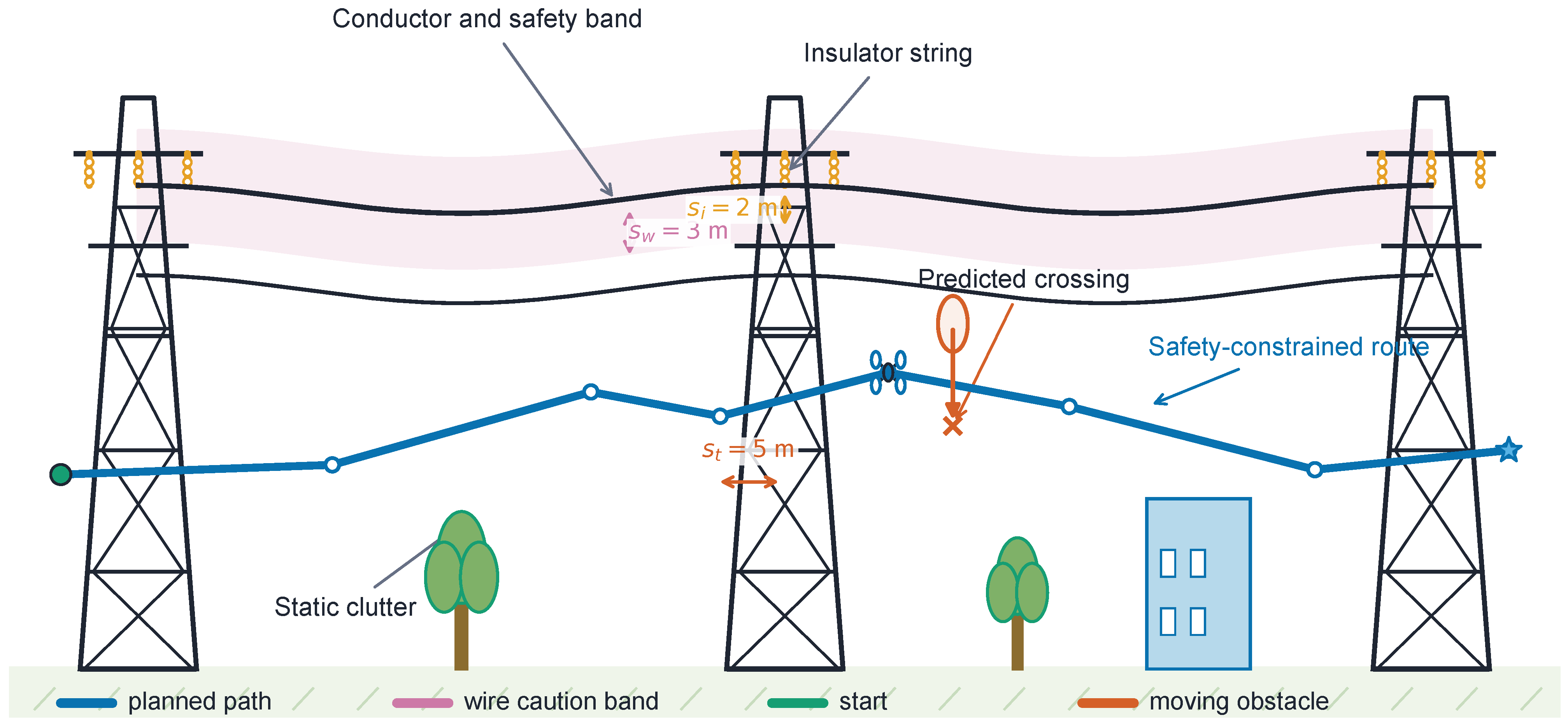
Figure 1 illustrates the physical elements represented in the planning model. The side elevation is schematic because tower clearance is evaluated in the horizontal plane, with the simulated route laterally offset from the tower axis. The conductor and its caution band affect both feasibility and risk, while trees, buildings, and predicted moving-obstacle positions influence waypoint selection.

The contributions are consolidated as follows:

• We formulate a power-line-specific feasible set that distinguishes conductor-line distance, tower-axis stand-off, tagged-insulator clearance, general-clutter surface clearance, and predicted moving-object clearance. A soft risk objective ranks only admitted edges, and the same sampled segment predicate is applied during graph search, line-of-sight smoothing, and final evaluation. Proposition 1 establishes sampled-feasibility preservation, within the stated sampling resolution, for any finite set of soft-risk weights.
• We provide an implementation-level description that includes a worked candidate calculation, pseudocode, explicit failure handling, an uncertainty margin for noisy velocity estimates, and a machine-readable parameter manifest. The formulation explicitly states the limitations of the sampled verifier and does not claim a continuous-time safety guarantee.
• We construct a paired simulation benchmark with six scenario families, three difficulty levels, five seeds, executable classical and hybrid baselines, controlled obstacle-count and occupied-volume-density factors, component ablations, one-at-a-time weight perturbations, and targeted tests of route crossings and prediction noise. An additional comparison imposes the same cap on hard-verifier point checks for every planner, thereby avoiding the assumption that an A* expansion, an RRT sample, and a DWA rollout are equivalent computational units. The configurations, seeds, trial-level records, analysis scripts, and publication figures are included as reproducibility artifacts.

The remainder of this paper is organized as follows. Section 2 positions the method relative to recent power-line, hybrid, dynamic, and risk-aware planners. Section 3 defines the simulator, risk and feasibility models, search procedure, baselines, metrics, and reproducibility protocol. Section 4 and Section 5 present the matched benchmark, density and ablation results, and dynamic-risk and sensitivity analyses. Section 6 summarizes the conclusions supported by these results and outlines the remaining steps from simulation to practical validation.

2. Related Work

2.1. Power-Line Inspection Planning

Power-line inspection combines asset detection, viewpoint selection, trajectory generation, and control. Reviews of UAV inspection and remote-sensing path planning report gains in access and repeatability but identify clearance management, perception uncertainty, and environmental variability as persistent limitations [8,9]. Recent outdoor inspection research has also adapted locally optimized trajectory generation to power-line environments and evaluated the resulting system in both simulation and flight [10]. Together with the graph-search and perception-aware studies introduced in Section 1, this body of work motivates the asset-specific geometry adopted here. Our scope is narrower than that of an end-to-end inspection system: the simulator supplies geometry and obstacle states, and the planner returns a sampled, collision-checked path.

2.2. Classical, Hybrid, Dynamic, and Learning Methods

A* search [11], asymptotically optimal sampling-based planning [12], artificial potential fields (APFs) [13], DWA [14], and bidirectional RRT-Connect [15] remain useful reference methods because their assumptions and computational trade-offs are well understood. Surveys describe how these families balance completeness, path quality, environmental knowledge, and online responsiveness [16,17]. Recent studies have often combined global and local components. Gao et al. fused enhanced A* search with an adaptive potential field [18]; Ahmed and Sheltami used receding-horizon optimization for three-dimensional collision avoidance [19]; and QuickNav combined global guidance with reactive collision handling [20]. These studies motivate the executable A*–DWA global–local baseline included in the matched comparison.

Learning-based planners can adapt to complex state distributions, and deep reinforcement learning has been investigated in large dynamic environments [21]. Direction-aware A* search has also been coupled with a PPO-derived heuristic [22]. Reported performance in such studies depends on the training budget, seed selection, and evaluation protocol [23]. The quantitative comparison in this study therefore includes only planners executed on every listed scenario; no proxy profile is presented as the result of a trained policy. Learning-based planning remains a relevant extension, but it is not used to support the present performance claims.

2.3. Risk-Aware Planning and Remaining Gap

Risk-aware methods have represented third-party exposure [24], GIS-derived target levels of safety [25], and autonomous planning in unknown complex environments [26]. Dynamic-planning studies have examined adaptive neighborhoods [27], while density-oriented tests have been used to evaluate RFA-star [28]. Path postprocessing has ranged from geometric Bézier refinement [29] to dynamically motivated trajectory generation [30].

Table 1. Positioning against representative recent UAV planning studies. “NR” means that the item was not reported as a primary evaluation factor in the cited study.

Study	Main Setting	Planning Approach	Power-Line Semantics	Dynamic Obstacles	Uncertainty/Noise	Validation
Li et al. (2024) [4]	Power-line inspection	Improved A*	Yes	No	NR	Simulation
He et al. (2024) [6]	Complex 3D environment	Optimized A*–DWA	No	Yes	NR	Simulation
Zhang et al. (2024) [28]	High-density agricultural scenes	RFA-star	No	No	NR	Density/map-size tests
Xu et al. (2025) [27]	Dynamic UAV planning	Adaptive-neighborhood A*	No	Yes	NR	Simulation
Zong et al. (2025) [7]	Unknown environment	Risk-aware planning	No	Environment risk	Risk model	Simulation
Braßel et al. (2025) [25]	Urban GIS routes	Safety-level-constrained optimization	No	No	GIS risk inputs	GIS case study
Lan et al. (2026) [10]	Outdoor power-line inspection	Improved EGO-planner	Yes	Obstacles	NR	Simulation and flight
PL-RiskPlanner	Synthetic power-line corridors	Safety-constrained risk-aware A* with verified smoothing	Yes	Arrival-time prediction	Velocity-noise margin	Paired simulation benchmark

compares the capabilities and validation settings of representative recent studies. The comparison is intentionally qualitative because path length and runtime measured on different maps or hardware are not directly comparable. In contrast, the matched numerical comparison in Section 4 executes every baseline implementation with the same geometry, safety checker, seeds, and workstation.

The methodological distinction lies in this separation of roles. Hard constraints define admissibility, soft asset-specific risk ranks admissible edges, approximate arrival-time prediction provides time-indexed dynamic geometry, and smoothing cannot bypass the verifier. The benchmark is a separate but complementary contribution because it tests these roles through shared-simulator baselines, ablations, density factors, and noise perturbations. Direct numerical comparisons of verified completion, safety flags, path length, clearance, and wall-clock query time are therefore restricted to the matched implementations in Section 4 and the accompanying supplementary tables.

3. Materials and Methods

3.1. Study Scope and Planning Problem

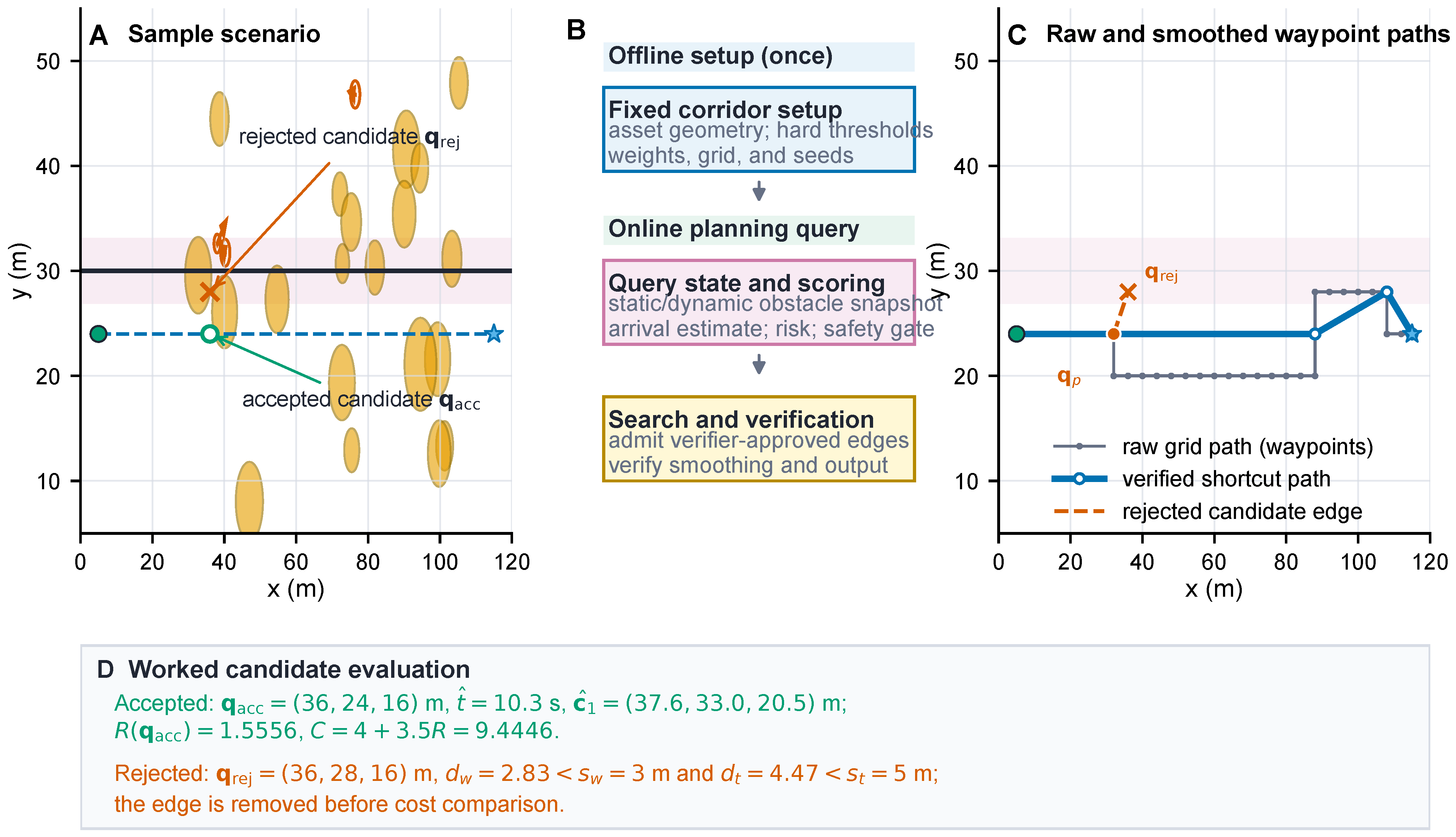
This study evaluates path planning in synthetic corridor geometry with obstacle states supplied to the planner. It does not model onboard perception, low-level flight control, wind, communication delay, or vehicle dynamics beyond a maximum-speed approximation of arrival time. The term “online” in Figure 2 denotes computation performed for a single planning query from a supplied obstacle-state snapshot; it does not imply a deployed real-time replanning system. Accordingly, PL-RiskPlanner is evaluated as a planner for power-line corridors, not as a universal obstacle-avoidance algorithm or a faster implementation of A*.

The workspace is $\mathcal{W}=[0,120]\times [0,60]\times [0,35]$ m. A planning state is the UAV-center position

$$\mathbf{q}={[x,y,z]}^{\top }\in \mathcal{W},$$

(1)

and a candidate path is an ordered sequence

$$\mathcal{P}=\{{\mathbf{q}}_0,{\mathbf{q}}_1,\dots ,{\mathbf{q}}_N\},$$

(2)

where ${\mathbf{q}}_0=(5,24,16)$ m and ${\mathbf{q}}_N=(115,24,16)$ m in the default corridor. The planning task is to connect these endpoints with segments that remain in $\mathcal{W}$ and satisfy all five sampled clearance inequalities in Equation (8), while minimizing the accumulated objective in Equation (10). The nominal inspection route is laterally displaced from a straight conductor located at $y=30$ m and $z=18$ m. Tower axes are located at $x\in \{0,40,80,120\}$ m and $y=30$ m. In the simulator, conductor distance is the perpendicular distance to the straight line, whereas tower distance is the horizontal distance to the nearest tower axis. The conceptual catenary in Figure 1 is not used in the numerical evaluation.

Conductors, towers, insulators, trees, buildings, and terrain are all kinematically static in the simulator. They are nevertheless represented as distinct semantic classes because their safety functions are not interchangeable. A conductor uses distance to a line and a conductor-specific stand-off; a tower uses horizontal distance to an axis; an insulator uses net clearance to a tagged sphere and its own threshold; and general static clutter denotes the remaining non-asset spherical proxies. Thus, “static obstacle” refers to general clutter unless a power asset is named explicitly; this distinction does not imply that conductors or towers move. In the implementation, every fixed spherical proxy, including each tagged insulator, also undergoes a generic non-contact check, with the stricter insulator threshold imposed in addition. Dynamic objects are represented as spheres with constant velocity vectors. Static and dynamic net clearances subtract both the obstacle radius and the UAV radius $r_u=0.35$ m, whereas conductor and tower thresholds are specified directly for the UAV center.

Figure 2 summarizes a complete planning query and includes a worked edge evaluation. In panel A, ${\mathbf{q}}_p$ denotes the predecessor grid state, ${\mathbf{q}}_{\mathrm{acc}}$ a candidate admitted by the hard verifier, and ${\mathbf{q}}_{\mathrm{rej}}$ a candidate rejected by that verifier. A waypoint is a retained three-dimensional vertex in an ordered path. In panel C, the raw grid path connects adjacent search waypoints. A verified shortcut connects non-consecutive raw waypoints only after SafeSeg accepts the segment. A rejected candidate edge fails the same predicate and is therefore excluded from both the search graph and the smoothed path. Section 3.4, Section 3.5 and Section 3.6 define the numerical entries and module interactions.

3.2. Scenario Families and Test Conditions

The generator deterministically constructs six scenario families from a family name, difficulty level, map index, and random seed.

Table 2. Synthetic scenario factors used in the matched benchmark.

Scenario Family	Dominant Generated Objects	Static-Count Bonus	Random Moving Objects
Straight corridor	Trees, buildings, terrain	0	No
Tower–insulator dense	Tower-adjacent objects, insulators, wire-risk objects	5	No
Tree intrusion	Trees and wire-risk objects	8	No
Building–terrain mixed	Buildings, terrain, trees	10	No
Dynamic-obstacle region	Trees, buildings, terrain	4	Yes
Heterogeneous mixed family	Trees, buildings, terrain, tower-adjacent objects	12	No

summarizes these factors. The three difficulty levels use base static-object counts of 8, 16, and 28, to which family-specific bonuses of 0–12 objects are added. Object classes are assigned cyclically in the order shown in Table 2. The tree-intrusion family follows the cycle tree–tree–wire-risk, whereas each other family cycles through its listed classes. Static centers are sampled as $x\sim \mathcal{U}(12,108)$ m and $y\sim \mathcal{U}(8,52)$ m. Heights follow $z\sim \mathcal{U}(14,22)$ m for tower-adjacent, insulator, and wire-risk objects, $z\sim \mathcal{U}(1,8)$ m for terrain, and $z\sim \mathcal{U}(3,24)$ m for trees and buildings. The base radii for trees, buildings, terrain, tower-adjacent objects, insulators, and wire-risk objects are 1.8, 3.0, 2.5, 2.0, 1.1, and 1.0 m, respectively. Each base radius is multiplied by the difficulty factor 1.00, 1.25, or 1.55 and by an independent draw from $\mathcal{U}(0.8,1.2)$.

Only the dynamic-obstacle family contains randomly generated moving objects in the general benchmark: 1, 3, or 5 objects at easy, medium, or hard difficulty, respectively. Their initial centers follow $x\sim \mathcal{U}(20,100)$ m, $y\sim \mathcal{U}(10,50)$ m, and $z\sim \mathcal{U}(10,23)$ m, while their radii follow $\mathcal{U}(0.6,1.4)$ m. Initial velocity components are sampled from $[-0.5,0.5]$ m/s in the x and y directions and $[-0.1,0.1]$ m/s in the z direction. The targeted route-crossing tests replace these random motions with controlled crossings near estimated UAV arrival times. For each generated map, the local pseudorandom generator is initialized by interpreting the first 16 hexadecimal digits of SHA-256(seed:family:difficulty:map-index) as an integer. Generated coordinates and radii are stored to three decimal places. This rule, the canonical family identifiers, and every ordered object list are retained in the released manifest and trial archive.

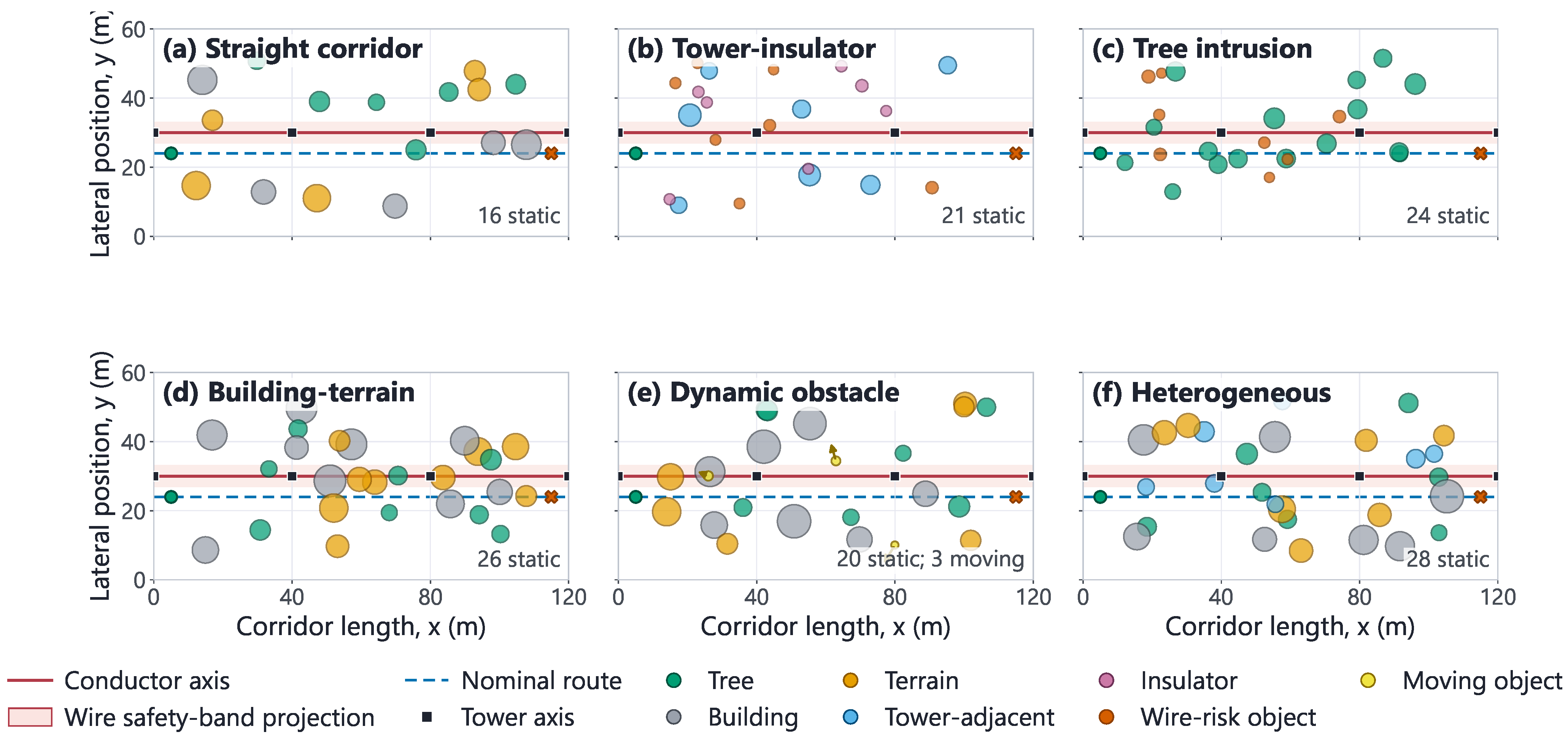
Figure 3 shows plan-view projections generated directly by the released scenario code for one matched, medium-difficulty condition. Each colored circle represents the horizontal footprint of a spherical obstacle proxy after addition of the UAV radius, and its color identifies the object class. The circular symbols in the legend denote the same classes but are not drawn to scale. In contrast, the pale annotated rectangle represents only the plan-view projection of the continuous conductor safety band; it is not another obstacle symbol. The tower–insulator and tree-intrusion families concentrate objects near power assets, the building–terrain family combines larger clutter classes, and the dynamic family adds moving objects marked with velocity vectors. Each object’s z coordinate remains active in the three-dimensional safety calculations and is not discarded by the planner.

The default safety distances are $s_w=3$ m from the conductor, $s_t=5$ m from a tower axis, and $s_i=2$ m of net clearance from tagged insulator spheres. The environment configuration also retains a 0.2 s integration step and an 800-step episode limit for compatibility with future control-policy studies; these values do not determine graph-search execution time.

3.3. Research Difficulties and Design Responses

The method addresses four specific difficulties in this planning problem. D1: Heterogeneous asset geometry. Conductors, tower axes, tagged insulators, and general clutter require distinct distance functions and thresholds. Equation (8) addresses this issue through an explicit five-part feasibility predicate. D2: Temporal coexistence. Spatial clearance alone does not reveal a route-crossing conflict. Equations (3) and (4) therefore introduce candidate-specific arrival-time prediction, with a bounded uncertainty margin when velocity estimates are noisy. D3: Constraint consistency. Unconstrained shortcutting can invalidate an edge that was accepted during search. The method therefore applies one sampled segment predicate during search, smoothing, and final evaluation, leading to Proposition 1. D4: Computational accountability. Repeated geometric checks increase query time, while algorithm-specific iteration counters are not directly comparable. We therefore report wall-clock time and expanded or sampled states and conduct an additional experiment with the same cap on hard-verifier point checks for every planner.

These design responses delimit the methodological contribution. PL-RiskPlanner does not alter the asymptotic A* search rule, nor do we claim that arrival-time prediction is novel in isolation. The contribution examined here is a testable, power-line-specific composition in which semantic constraints define admissibility, soft risk affects preference only within the feasible set, and postprocessing cannot bypass the sampled checker. The route-crossing tests address D2, the component ablation addresses D3, and the density, weight, and equal-budget analyses examine D1 and D4.

3.4. PL-RiskPlanner Workflow

PL-RiskPlanner combines five modules: approximate arrival-time prediction, a power-line risk field, a hard point-and-segment verifier, six-connected risk-aware A* search, and verifier-gated line-of-sight smoothing. The method is hybrid in composition because it couples discrete global search, time-indexed obstacle prediction, hard geometric screening, and geometric postprocessing; “hybrid” does not denote a new A* expansion rule.

Figure 2 provides a worked example from the medium-difficulty dynamic-obstacle scenario with map index 1 and seed 0. Starting from the predecessor ${\mathbf{q}}_p=(32,24,16)$ m, the candidate ${\mathbf{q}}_{\mathrm{acc}}=(36,24,16)$ m has an estimated arrival time of 10.3 s and a risk value of 1.5556, which gives an edge cost of 9.4446. The alternative ${\mathbf{q}}_{\mathrm{rej}}=(36,28,16)$ m is rejected before cost comparison because its conductor and tower distances are 2.83 m and 4.47 m, respectively, both below their hard thresholds. Panel C further shows that non-consecutive raw waypoints are connected only when the proposed shortcut passes SafeSeg. The dashed orange edge represents a rejected proposal and is not part of either returned path.

3.5. Dynamic Prediction, Risk Field, and Hard Feasibility

For a candidate state $\mathbf{q}$, the approximate arrival time is computed from the straight-line distance to the start and the configured maximum speed $v_{max}=3$ m/s:

$$\widehat{t}\left(\mathbf{q}\right)={\displaystyle \frac{{\parallel \mathbf{q}-{\mathbf{q}}_0\parallel }_2}{v_{max}}}.$$

(3)

This low-cost estimate does not integrate distance along the partially constructed path and can therefore differ from the arrival time during dynamic execution. For a moving object j with center ${\mathbf{c}}_j$, velocity ${\mathbf{v}}_j$, and radius $r_j$, the predicted center is

$${\widehat{\mathbf{c}}}_j\left(\mathbf{q}\right)={\mathbf{c}}_j+{\mathbf{v}}_j\widehat{t}\left(\mathbf{q}\right).$$

(4)

When the relative standard deviation of a velocity estimate is ${\sigma }_v$, the optional radial uncertainty margin is

$${\mu }_j\left(\mathbf{q}\right)=min\left({\mu }_{max},z{\sigma }_v{\parallel {\mathbf{v}}_j\parallel }_2\widehat{t}\left(\mathbf{q}\right)\right),$$

(5)

where $z=2.0$ and ${\mu }_{max}=6$ m by default in the uncertainty-aware tests. The margin is set to zero in the nominal matched benchmark. Dynamic net clearance is obtained by subtracting $r_j$, $r_u$, and ${\mu }_j$ from the distance between the candidate state and the predicted center.

Let $d_w$, $d_t$, $d_i$, $d_s$, $d_d$, and $d_r$ denote conductor distance, tower-axis distance, net tagged-insulator clearance, minimum net clearance to any fixed spherical proxy (including tagged insulators), predicted dynamic-object clearance, and deviation from the nominal inspection route. A normalized caution function is

$$\varphi (d;s,c)=\left\{\begin{array}{cc}1,\hfill & d\le s,\hfill \\ {\left({\displaystyle \frac{c-d}{c-s}}\right)}^2,\hfill & s<d<c,\hfill \\ 0,\hfill & d\ge c,\hfill \end{array}\right.$$

(6)

where s is the hard boundary and c is the caution distance. Conductor and tower caution distances are $2s_w$ and $2s_t$; static and dynamic caution clearances are 3 m. The soft field is

$$\begin{array}{cc}\hfill R\left(\mathbf{q}\right)=& w_w\varphi (d_w;s_w,2s_w)+w_t\varphi (d_t;s_t,2s_t)\hfill \\ \hfill & +w_s\varphi (d_s;0,3)+w_d\varphi (d_d;0,3)+w_r{d}_r.\hfill \end{array}$$

(7)

The default weights are $w_w=4.0$, $w_t=5.0$, $w_s=6.0$, $w_d=5.0$, and $w_r=0.08$. These values are prespecified engineering scaling coefficients rather than fitted probabilities. Each proximity term is dimensionless and bounded in $[0,1]$, so coefficients between 4 and 6 place the four asset and obstacle terms on a comparable scale. Route deviation is measured in meters and therefore receives the smaller coefficient of 0.08, preventing a meter-scale offset from dominating the bounded proximity terms. The defaults were fixed before the formal benchmark and were not optimized for individual scenarios or adjusted after inspection of the test outcomes. Because tagged insulators belong to the fixed-sphere pool used to compute $d_s$, they contribute to the generic static-risk term through $w_s$; the separate $d_i$ check imposes their asset-specific hard stand-off.

Soft risk never replaces feasibility. The five explicit clearance constraints have different meanings: $d_w\ge s_w$ enforces conductor-line stand-off, $d_t\ge s_t$ enforces horizontal tower-axis stand-off, $d_i\ge s_i$ enforces tagged-insulator surface clearance, $d_s>0$ prevents contact with every fixed spherical proxy, and $d_d>0$ prevents contact with a moving-object sphere at the predicted arrival time. The $d_s$ check therefore includes a zero-clearance contact test for insulators, while $d_i\ge s_i$ imposes the stricter tagged-insulator threshold. Together with the workspace bound, a point is admitted only when

$$\begin{array}{cc}\hfill Safe\left(\mathbf{q}\right)=1⟺& \mathbf{q}\in \mathcal{W},d_w\left(\mathbf{q}\right)\ge s_w,d_t\left(\mathbf{q}\right)\ge s_t,\hfill \\ \hfill & d_i\left(\mathbf{q}\right)\ge s_i,d_s\left(\mathbf{q}\right)>0,d_d\left(\mathbf{q}\right)>0.\hfill \end{array}$$

(8)

A segment is accepted only if every sampled point passes Equation (8):

$$SafeSeg({\mathbf{q}}_a,{\mathbf{q}}_b)=\prod _{\mathbf{q}\in S({\mathbf{q}}_a,{\mathbf{q}}_b)}\mathbb{I}\left[Safe\left(\mathbf{q}\right)=1\right],$$

(9)

where S includes both endpoints and at least one interior point, with a sample spacing no greater than 0.5 m. The search, final metric computation, and smoothing stages all call the same function. This sampled test provides a reproducible numerical verifier, but it does not prove continuous-time collision avoidance between samples.

3.6. Risk-Aware Search and Safety-Verified Smoothing

The global search uses a 4 m, six-connected Cartesian grid with a Euclidean heuristic. For adjacent states, the edge cost is

$$C({\mathbf{q}}_i,{\mathbf{q}}_j)={\parallel {\mathbf{q}}_j-{\mathbf{q}}_i\parallel }_2+\lambda R\left({\mathbf{q}}_j\right),\lambda =3.5,$$

(10)

subject to $SafeSeg({\mathbf{q}}_i,{\mathbf{q}}_j)=1$. The search stops when it reaches the goal or expands 20,000 nodes. If no goal path is found, the run is recorded as a planning failure, not automatically as a safety violation.

After the search, greedy line-of-sight smoothing tests the farthest remaining waypoint first. A shortcut is accepted only when it satisfies Equation (9); otherwise, the candidate endpoint is moved backward until a safe shortcut is found. During final whole-path verification, the planner falls back to the raw grid path if the smoothed result fails. Algorithm 1 summarizes this procedure.

Algorithm 1: PL-RiskPlanner for one obstacle-state snapshot.

Require: Scenario $\mathcal{S}$, start ${\mathbf{q}}_0$, goal ${\mathbf{q}}_g$, grid spacing h, weights, $\lambda$ Ensure: A verified path $\mathcal{P}$ or a planning-failure record   1: Construct the risk field and hard verifier from $\mathcal{S}$   2: Initialize the A* frontier with ${\mathbf{q}}_0$   3: while frontier is not empty and expanded nodes $<20,000$ do   4:     Pop the state with minimum accumulated cost plus Euclidean heuristic   5:     for each of its six grid neighbors ${\mathbf{q}}_j$ do   6:         Estimate $\widehat{t}\left({\mathbf{q}}_j\right)$ and predicted moving-object centers   7:         if $\neg Safe\left({\mathbf{q}}_j\right)$ or $\neg SafeSeg({\mathbf{q}}_i,{\mathbf{q}}_j)$ then   8:            continue   9:         end if 10:         Relax the edge using Equation (10) 11:     end for 12: end while 13: if the goal was not reached then 14:     return failure 15: end if 16: Reconstruct the raw grid path ${\mathcal{P}}_{\mathrm{raw}}$ 17: Greedily accept only shortcuts that pass SafeSeg 18: Verify the complete smoothed path; otherwise use ${\mathcal{P}}_{\mathrm{raw}}$ 19: return the verified path and sampled-clearance metrics

Proposition 1 (sampled-feasibility preservation).

Assume that PL-RiskPlanner returns a path $\mathcal{P}$ after its final verification. Every point in the segment sample set ${\bigcup }_{i=0}^{N-1}S({\mathbf{q}}_i,{\mathbf{q}}_{i+1})$ satisfies Equation (8), irrespective of the finite values assigned to λ and the five soft-risk weights.

Proof. 

Search inserts an edge only after SafeSeg returns 1. Smoothing replaces a subsequence only with an edge for which the same predicate also returns 1, and final verification checks every retained edge again. The risk terms are evaluated only after this admissibility test and therefore cannot authorize an infeasible edge. This property is limited to the stated 0.5 m sampling resolution and should not be interpreted as a continuous-time safety certificate.   □

For V expanded grid vertices and $E\le 6V$ neighbor edges, priority-queue search has the usual $O\left(\right(V+E)logV)$ graph overhead. If M objects and at most K segment samples are checked per edge, geometry evaluation contributes $O\left(EKM\right)$. Greedy smoothing is $O\left(N^{2}KM\right)$ in the worst case for an N-waypoint raw path. Expanded nodes, wall-clock query time, and raw/final waypoint counts are therefore reported alongside path metrics.

3.7. Executable Baselines, Ablations, and Parameters

The matched benchmark contains only algorithms that are executed for every listed trial: standard A* [11], RRT* [12], RRT-Connect [15], APF [13], DWA [14], risk-aware A*, an A*–DWA global–local hybrid [6], and PL-RiskPlanner. All baseline implementations receive the same scenario geometry and use the same hard point-and-segment verifier. They are shared-simulator implementations of algorithmic families, not claims of exact reproduction of every cited paper.

Table 3. Planner settings and algorithm-native stopping rules used in the matched simulator. Iteration-like counters are reported for reproduction and are not treated as equivalent compute units.

Planner	Main Mechanism	Algorithm-Native Stopping Rule and Fixed Parameters
Shared verifier	Hard point and segment admissibility	0.5 m maximum segment-sample spacing; common conductor, tower, insulator, static, and dynamic checks
A* [11]	Six-connected shortest-path grid search	4 m grid; 20,000-node limit; soft-risk weight 0
Risk-aware A* [11]	A* with the shared risk field	4 m grid; global risk weight 3.0; 20,000-node limit
PL-RiskPlanner	Risk-aware A* plus verified smoothing	4 m grid; global risk weight 3.5; weights $(4,5,6,5,0.08)$; 20,000-node limit
RRT* [12]	Goal-biased sampled tree with rewiring	220 samples; 6 m step; 12 m rewiring radius; goal every eighth sample
RRT-Connect [15]	Bidirectional connect search	400 samples; 6 m step; 0.70 corridor-sampling probability; 64 connect extensions
APF [13]	Greedy attractive/risk potential	90 moves; 3.5 m step; risk gain 2.0; 27 candidate directions
DWA [14]	Local three-step command rollout	90 moves; 4 m step; horizon 3; 27 commands
A*–DWA [6]	A* guide with local DWA rollouts	4 m grid; 140 local moves; 4 m step; horizon 3; 60 commands; two-node guide look-ahead

gives the complete primary settings; secondary score coefficients and all defaults are archived in configs/planner_parameters.toml. No planner was retuned separately for a test family. The A*–DWA implementation follows the global-guide/local-rollout pattern summarized in Section 2, and RRT-Connect provides a bidirectional sampling comparison. The native stopping counters in the final column are mechanism-specific safeguards, not a common compute unit: one A* node expansion, one RRT sample, and one DWA command rollout invoke different numbers of geometric checks. They are retained for exact reproduction, while the equal-verifier-budget experiment described below provides the resource-matched comparison requested for computational fairness.

The component ablation either sets the global multiplier $\lambda$ to zero (thereby disabling all soft-risk guidance), removes the tower soft term, removes the dynamic soft term, or disables smoothing while retaining the hard verifier. The archived identifier for the first condition is without_powerline_risk_field, but the figures and tables label it “w/o soft-risk guidance” to describe the implemented intervention precisely. Arrival-time prediction is examined separately in the controlled route-crossing experiment because randomly moving objects do not necessarily create a temporal conflict. In particular, “without tower cost” does not remove the hard tower-clearance constraint, and “without dynamic risk” removes only the soft dynamic term while retaining the predicted dynamic-obstacle admissibility checks. This distinction allows the ablation to test soft guidance without changing the feasible set implicitly.

3.8. Experimental Design

The main matched benchmark contains 6 families × 3 difficulty levels × 20 map indices × 5 seeds $=1800$ paired scenario instances. Executing 8 planners produces 14,400 trial records. Instances are paired by family, difficulty, map index, and seed. For a given key, every planner receives the same workspace, start and goal, conductor and tower geometry, ordered static-object list, moving-object states, radii, and safety thresholds. The component ablation applies five planner configurations to the same 1800 instances, producing 9000 additional records.

The resource-matched audit uses the same six families and three difficulty levels, map indices 0–4, seeds 0–4, and all eight planners, giving $6\times 3\times 5\times 5\times 8=3600$ additional trials. Each query is capped at 60,000 calls to the common point-level hard verifier, and every sampled point in a segment check consumes one unit of this budget. A query that reaches the cap before returning a verified path is recorded as a planning-only budget exhaustion rather than as a collision or safety violation. An algorithm may terminate earlier after reaching the goal, and the audit does not imply an equal number of floating-point operations outside the verifier. Instead, it imposes the same upper bound on calls to the shared, obstacle-dependent safety primitive and reports both the number of checks consumed and the wall-clock time.

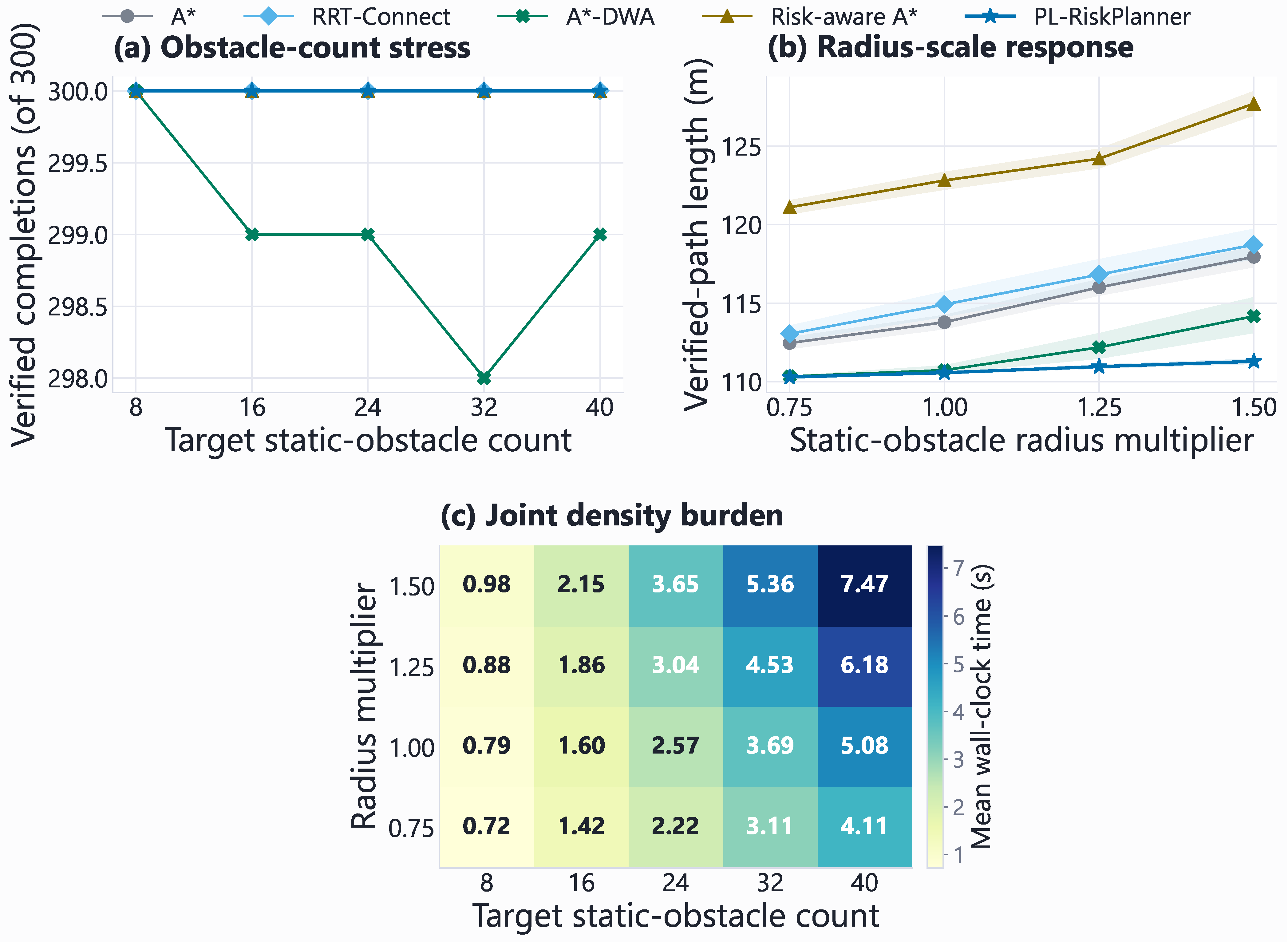
The controlled static-density experiment isolates obstacle burden at medium difficulty. It uses three clutter-focused families, five map indices, five target counts $\{8,16,24,32,40\}$, four radius multipliers $\{0.75,1.00,1.25,1.50\}$, five planners, and five seeds, producing 7500 rows. Within each family–map–seed tuple, all conditions share one canonical ordered list of obstacle centers: count selects a prefix and radius multiplier changes radii only. The reported nominal occupied-volume fraction is

$${\rho }_{\mathrm{nom}}={\displaystyle \frac{{\sum }_{k=1}^n\frac{4}{3}\pi {(r_k+r_u)}^3}{120\times 60\times 35}}.$$

(11)

Because overlapping spheres are not unioned, ${\rho }_{\mathrm{nom}}$ is a controlled density index rather than an exact free-space fraction.

The component-weight experiment uses one default condition and one-at-a-time perturbations of $\pm 25\%$ for $w_w,w_t,w_s,w_d,w_r$. Six families, three difficulty levels, five map indices, eleven conditions, and five seeds yield 4950 records. This range was selected to examine reasonable calibration variation around the fixed defaults rather than to search for a post hoc optimum.

The targeted route-crossing test uses the dynamic-obstacle family at all 3 difficulty levels, 20 map indices, and 5 seeds. It places 2, 4, or 6 moving objects near the nominal route at estimated UAV arrival times, samples their speeds from $[0.8,1.4]$ m/s, and evaluates PL-RiskPlanner, the no-prediction variant, and the no-dynamic-risk variant. This design produces 900 records. The prediction-noise test uses the same 60 maps and 5 seeds, 4 planner variants, and relative velocity-noise standard deviations ${\sigma }_v\in \{0,0.1,0.2,0.3,0.4\}$, producing 6000 records. Independent Gaussian noise with a component-wise standard deviation of ${\sigma }_v{\parallel {\mathbf{v}}_j\parallel }_2$ is added only to the velocity supplied to the planner. Clearance is then recomputed using the unperturbed moving-object velocities and the same approximate-arrival-time convention; this quantity is termed the simulator-reference dynamic clearance.

The uncertainty-margin sweep uses ten map indices per difficulty level, five seeds, noise levels $\{0.2,0.3,0.4\}$, multipliers $z\in \{1.5,2.0,2.5\}$, and caps ${\mu }_{max}\in \{4,6,8\}$ m, producing 4050 records. The setting $z=2.0$, ${\mu }_{max}=6$ m is the prespecified reference. These dynamic experiments are reported separately from the nominal benchmark to avoid generalizing results from controlled crossings or noisy velocity estimates to untested conditions.

3.9. Metrics and Statistical Analysis

The metric definitions separate four events:

• Planner-reported success: the planner returns a goal-reaching path according to its own termination and internal checks.
• Collision: sampled static or dynamic net clearance is non-positive.
• Safety violation: any sampled conductor, tower, insulator, static, or dynamic clearance violates Equation (8). A collision is therefore also a safety violation, but a search-budget failure is not.
• Verified completion: planner-reported success with neither collision nor safety violation under the independent final evaluator. A planning-only failure is a non-completion without a recorded safety violation.

Path length is

$$L\left(\mathcal{P}\right)={\displaystyle \sum _{i=0}^{N-1}}{\parallel {\mathbf{q}}_{i+1}-{\mathbf{q}}_i\parallel }_2.$$

(12)

To avoid rewarding a short path that does not pass final verification, the primary composite cost is   

$$\begin{array}{cc}\hfill J_{\mathrm{safe}}\left(\mathcal{P}\right)=& L\left(\mathcal{P}\right)\hfill \\ \hfill & +\alpha \mathbb{I}\left[\mathrm{not}\mathrm{a}\mathrm{verified}\mathrm{completion}\right],\hfill \end{array}$$

(13)

with $\alpha =1000$ m. Smoothness matches the released implementation:

$$S\left(\mathcal{P}\right)={\displaystyle \sum _{i=1}^{N-1}}\left(1-{\displaystyle \frac{\Delta {\mathbf{q}}_{i-1}^{\top }\Delta {\mathbf{q}}_i}{{\parallel \Delta {\mathbf{q}}_{i-1}\parallel }_2{\parallel \Delta {\mathbf{q}}_i\parallel }_2}}\right),$$

(14)

where zero-length segments are skipped. The reported energy value $0.1L+0.5S$ is a geometric proxy, not measured electrical energy.

For a returned path, the minimum safety margin is the smallest value, over all sampled path points, among the conductor distance minus $s_w$, tower distance minus $s_t$, tagged-insulator net clearance minus $s_i$, minimum net clearance to fixed spherical proxies, and dynamic-object net clearance. This common margin is positive only when every asset-specific sampled threshold is satisfied.

Path geometry, the energy proxy, clearance, smoothness, and search-size summaries are calculated only for verified completions. Wall-clock query time and $J_{\mathrm{safe}}$ are calculated over all trials. The timer starts immediately before deterministic scenario construction and stops when the planner returns. It therefore includes shared scenario preparation and planner-specific search and postprocessing but excludes the independent post hoc metric calculation. Algorithms are interleaved within each scenario key under the same guarded worker schedule. The resulting end-to-end times are descriptive matched measurements rather than isolated search-kernel benchmarks. In the route-crossing and velocity-noise analyses, simulator-reference dynamic clearance is also summarized over planner-returned paths before independent safety filtering, so unsafe returned paths are not hidden by complete-case selection. Outcome proportions receive Wilson 95% intervals, while mean paired differences relative to PL-RiskPlanner receive percentile-bootstrap 95% intervals from 2000 resamples using analysis seed 20260731. The complete analysis policy is stored in configs/major_revision_analysis.toml. Raw proportions are retained in the archive but are displayed in the manuscript as counts, percentages, or concise decimal values without unnecessary trailing zeros.

3.10. Implementation and Reproducibility

Experiments run on Windows 11 (build 10.0.26200; Microsoft Corporation, Redmond, WA, USA) with an Intel Core Ultra 7 270K Plus CPU (Intel Corporation, Santa Clara, CA, USA) (24 physical cores and 24 logical processors), 63.4 GB usable RAM, and an NVIDIA GeForce RTX 5090 D v2 (NVIDIA Corporation, Santa Clara, CA, USA) with 24,455 MiB memory. The planners execute on the CPU; the GPU is reported for workstation completeness and is not used to accelerate the graph or sampling planners. The software environment is Python 3.12.10, NumPy 2.4.6, pandas 3.0.3, SciPy 1.17.1, and Matplotlib 3.11.0.

Formal experiments use five seeds (0–4), process pools of at most four workers, periodic CSV checkpoints, and a resource guard that terminates a run if CPU utilization, system-memory use, GPU utilization, or GPU-memory use exceeds 90%. The run manifest records commands, package versions, workstation information, and SHA-256 hashes of the evaluated source and configuration files. The accompanying reproducibility archive contains configs/, src/, scripts/, trial-level CSV files, summary tables, figure-generation code, and the exact random seeds.

OpenAI Codex (GPT-5, OpenAI, San Francisco, CA, USA; accessed June–July 2026) assisted with experimental-protocol structuring, code editing, analysis-script organization, figure-layout refinement, and manuscript language. All formal numerical records reported here were computed by the archived local Python scripts from the stated configurations and seeds rather than accepted from model-generated text. The authors reviewed the code, numerical outputs, figures, and interpretations and remain responsible for this study.

4. Matched Benchmark and Static-Obstacle Robustness

4.1. Matched Comparison with Executable Baselines

Table 4. Matched-simulator benchmark results pooled across the six families in Table 2, three difficulty levels, map indices 0–19, and seeds 0–4 (1800 paired scenario keys per planner). Path length and the path-level minimum safety margin are summarized over verified completions, whereas wall-clock query time and safety-penalized cost are calculated over all trials.

Planner	Verified Completions	Planning-Only Failures	Safety Flags	Path Length (m)	Minimum Safety Margin (m)	Wall-Clock Time (s)	${\mathit{J}}_{\mathbf{safe}}$ (m)
A* [11]	1800/1800	0	0	114.96 ± 528	0.66 ± 39	0.366 ± 529	114.96
RRT* [12]	1788/1800	12	0	116.13 ± 355	0.63 ± 64	0.203(151)	122.74
RRT-Connect [15]	1800/1800	0	0	115.95 ± 744	0.50 ± 50	0.045 ± 21	115.95
APF [13]	1800/1800	0	0	116.84 ± 254	2.10 ± 68	0.496 ± 170	116.84
DWA [14]	1800/1800	0	0	110.80 ± 92	0.72 ± 35	1.058 ± 353	110.8
A*–DWA [6]	1799/1800	1	0	111.78 ± 770	0.73 ± 37	2.764 ± 1315	112.38
Risk-aware A* [11]	1800/1800	0	0	123.78 ± 640	1.78 ± 73	3.120 ± 2461	123.78
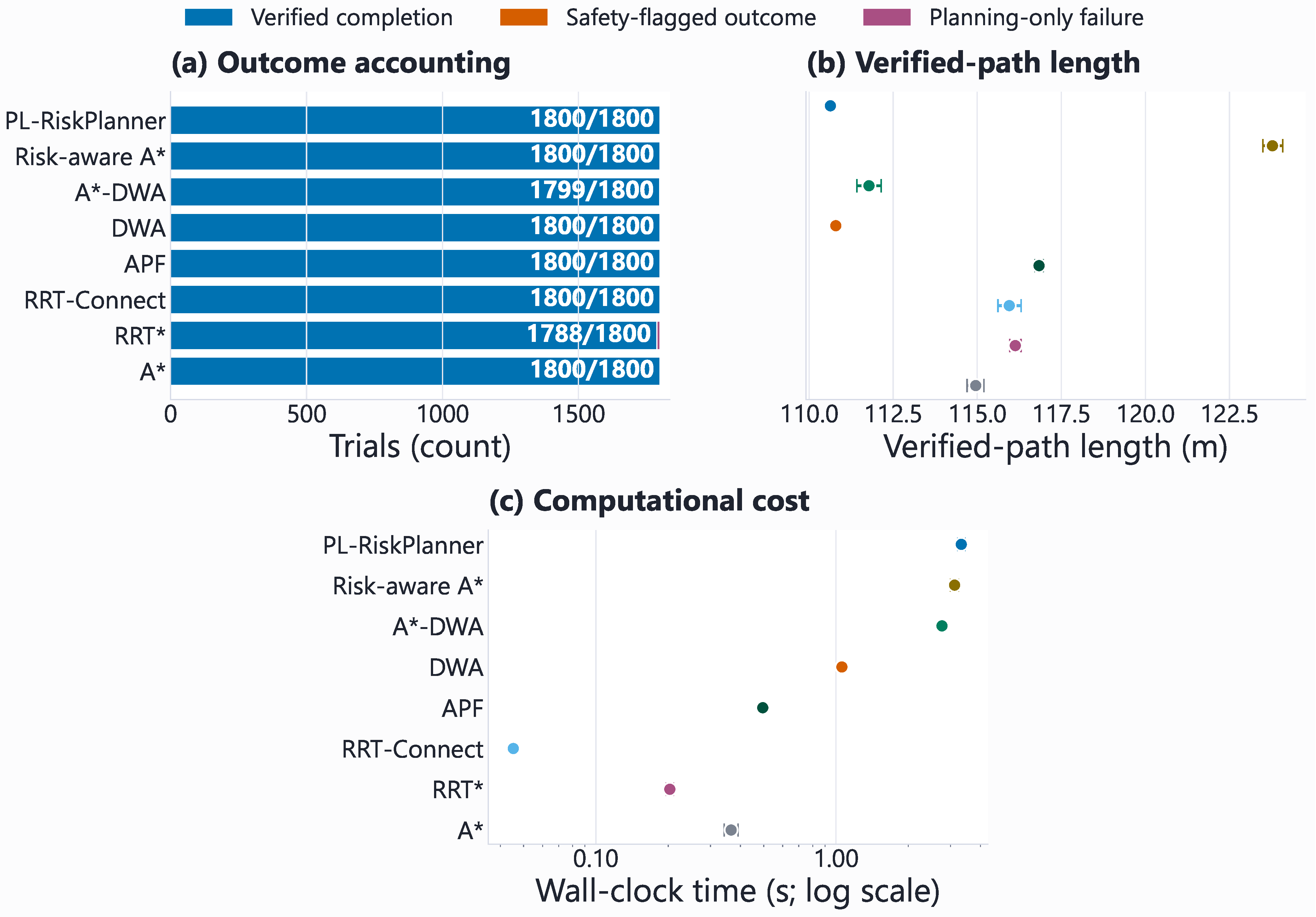
PL-RiskPlanner	1800/1800	0	0	110.64 ± 104	0.67 ± 47	3.327 ± 2541	110.64

reports results for the eight planners under identical scenario keys and distinguishes verified completions, planning-only failures, and safety flags. The table pools all six families in Table 2, all three difficulties, map indices 0–19, and seeds 0–4. This gives 1800 fully specified keys for each planner. Within each key, the start, goal, workspace, conductor and tower geometry, ordered object lists, radii, velocities, and clearance thresholds are identical across algorithms; only the planning algorithm changes. The released row identifiers and scenario generator allow every pooled entry to be reproduced, rather than only the representative maps in Figure 3. Across 1800 nominal matched trials for PL-RiskPlanner, no safety flag was recorded under the independent evaluation; the corresponding verified-completion and planning-only-failure counts are reported in the table. The absence or rarity of an observed flag is not treated as certainty: the Wilson 95% upper bound for the underlying PL-RiskPlanner flag probability is 0.21% under this protocol. Its mean path length among verified completions was 110.64 ± 1.04 m, its mean minimum safety margin was 0.67 ± 0.47 m, and its mean wall-clock query time over all trials was 3.327 s.

The similar mean path lengths of DWA and PL-RiskPlanner call for a trade-off analysis rather than a dominance claim. Across all 1800 paired keys, the mean path-length difference (DWA minus PL-RiskPlanner) was 0.160 m (95% paired-bootstrap CI [0.123, 0.199] m), indicating only a small geometric difference. DWA’s mean sampled minimum safety margin was 0.043 m greater (95% CI [0.022, 0.064] m), and its mean query time was 2.268 s shorter (95% CI [2.167, 2.372] s). In contrast, PL-RiskPlanner produced lower values for the lower-is-better smoothness measure: the mean difference (DWA minus PL-RiskPlanner) was 0.180 (95% CI [0.168, 0.192]). It also returned 25.91 fewer waypoints on average (95% CI [25.89, 25.94]) and reduced the energy proxy by 0.106 (95% CI [0.097, 0.115]). Thus, PL-RiskPlanner does not supersede DWA in either speed or sampled margin. Its observed advantage is a compact, globally searched route whose shortcuts are rechecked by the asset-specific predicate, whereas the tested DWA implementation provides lower-latency local rollouts with more returned waypoints. These roles could be combined in a future planning stack, although such integration lies outside the present simulation benchmark.

Figure 4 complements the exact table by addressing three questions. Panel (a) shows how each trial was accounted for rather than compressing outcomes into a rounded rate. Panel (b) compares path length only where the final evaluator accepted the path, and panel (c) shows the computational cost on a logarithmic axis. Among matched cases completed by both methods, the mean paired path-length difference (DWA minus PL-RiskPlanner) was 0.16 m (95% bootstrap CI [0.12, 0.2] m); their aggregate verified-path means were 110.8 and 110.64 m, respectively. This comparison concerns the shared simulator and parameter budgets in Table 3; it is not a claim that one implementation dominates every variant of the corresponding algorithmic family.

PL-RiskPlanner is not the fastest method in computational terms. Its additional query time is consistent with three-dimensional risk-weighted expansion, predicted moving-object queries at sampled states, the common segment verifier, and farthest-first shortcut checks after search. Reporting expanded nodes and raw and returned waypoint counts in Supplementary Table S3 supports this explanation rather than attributing the runtime to unspecified implementation overhead. Section 4.3 further isolates the expansion burden associated with the complete soft-risk guidance.

Table 5. Equal-verifier-budget audit with a maximum of 60,000 hard-safety point checks per query (450 paired trials per planner). Path length is summarized over each planner’s verified completions and is not compared across unequal completion subsets; the number of checks and query time are calculated over all trials.

Planner	Verified	Budget Exhausted	Other Failures	Mean Point Checks	Mean Time (s)	Verified Path Length (m)
A* [11]	450/450	0	0	5739	0.395	114.98
RRT* [12]	448/450	0	2	3737	0.225	115.96
RRT-Connect [15]	450/450	0	0	623	0.048	115.63
APF [13]	450/450	0	0	8516	0.531	116.86
DWA [14]	450/450	0	0	18,696	1.133	110.80
A*–DWA [6]	407/450	43	0	46,804	2.868	110.64
Risk-aware A* [11]	317/450	133	0	43,343	2.729	120.83
PL-RiskPlanner	292/450	158	0	45,577	2.836	110.21

separates this cost from the incomparable native counters in Table 3. Every algorithm receives the same upper bound on calls to the common obstacle-dependent point verifier; early goal completion remains allowed. Within this cap, PL-RiskPlanner completed 292/450 queries and exhausted the budget in 158, whereas DWA completed 450/450 queries without exhausting the budget. The two planners consumed a mean of 45,577 and 18,696 point checks per query, respectively. This audit is deliberately interpreted as a shared safety-query budget, not as proof that all non-verifier operations have identical cost.

The strict cap exposes, rather than eliminates, the method’s computational trade-off: PL-RiskPlanner exhausted the shared budget in 158 of 450 queries, whereas DWA did not exhaust the budget. The conditional path means in Table 5 are not used to support a superiority claim because the completion subsets differ. Together with the unrestricted native-termination times in Table 4, the audit shows that the asset-specific global search and verified shortcutting require more safety queries than DWA. This cost is compatible only with planning settings whose latency budget permits multi-second queries; reducing verifier calls and incremental replanning remain future work.

4.2. Controlled Obstacle Count and Radius

The factorial density experiment examines whether the main ordering persists as clutter increases in a controlled manner. Figure 5 separates the target object count from the radius multiplier and uses a joint heat map for PL-RiskPlanner’s wall-clock query time. At the most demanding tested cell (40 objects and radius multiplier 1.5), PL-RiskPlanner produced 75/75 verified completions. At this cell, no safety flag was recorded; its mean verified path length and all-trial wall-clock query time were 112.25 m and 7.47 s. For reference, the corresponding values at 8 objects and multiplier 0.75 were 110.12 m and 0.72 s. The controlled increase in clutter therefore added 2.14 m to the mean verified-path length while multiplying wall-clock query time by 10.4; the computational effect was larger than the geometric change over this tested range.

The heat-map cells should be read together with the outcome panels. A short path or low runtime is not evidence of robustness if the corresponding trial does not pass final verification. Full count-wise, radius-wise, and joint-cell values are retained in Supplementary Table S4a,b rather than adding another large table to the main text.

4.3. Component Ablation and Verified Smoothing

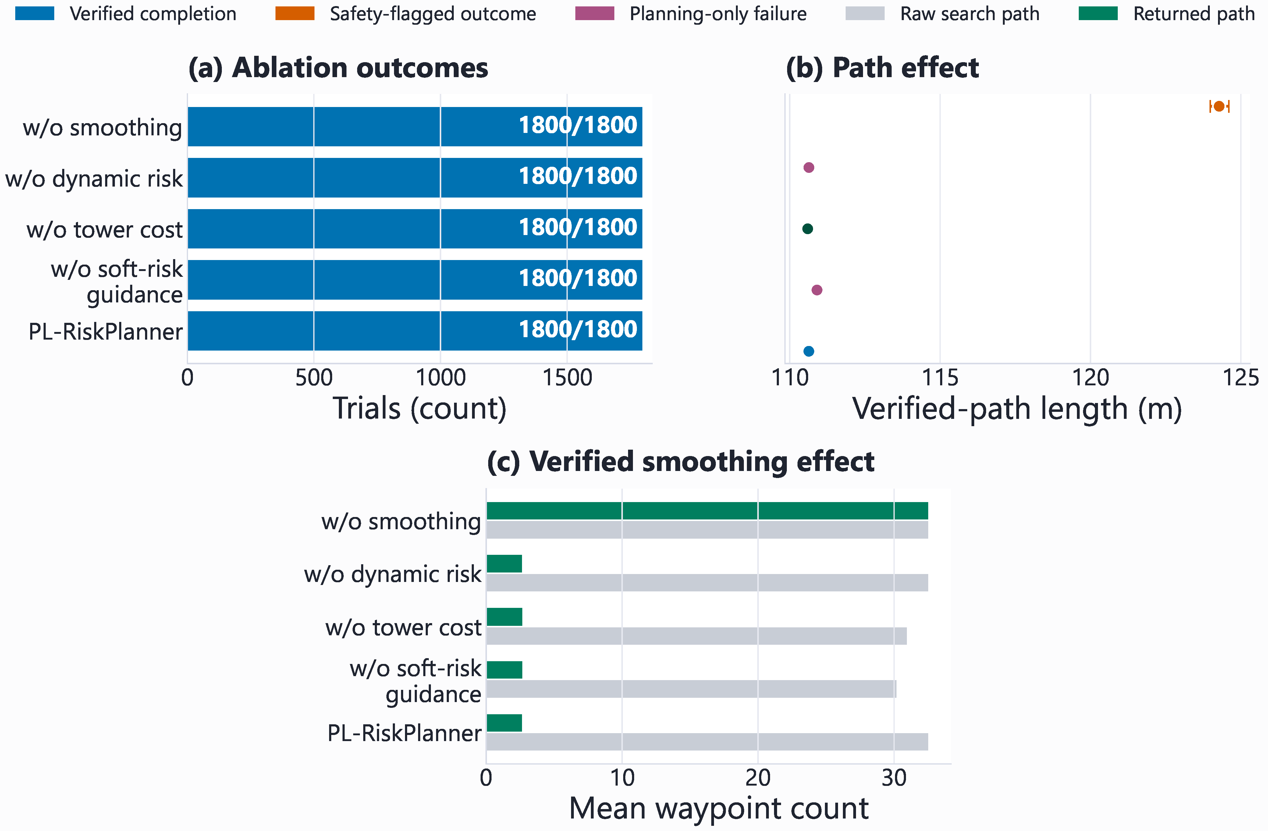
Figure 6 attributes observed changes to the soft field, tower and dynamic soft terms, and postsearch smoothing while leaving the hard feasible set unchanged. The clearest effect on path geometry is associated with smoothing: the no-smoothing configuration returned a mean path of 124.28 m, compared with 110.64 m for the complete method, a difference of 13.64 m (95% paired-bootstrap CI [13.37, 13.91] m). In the complete method, the raw grid path contained 32.6 waypoints on average and the verified returned path contained 2.7.

The ablation does not establish that every soft term is universally necessary. Instead, it shows how each term changes path preference or search burden under a fixed hard checker. In particular, the smoothing result supports the role of verified postprocessing in improving path efficiency: it removes grid-induced detours without authorizing a shortcut that was not independently sampled and checked. The complete soft-risk guidance produced a different trade-off: the complete planner expanded 950.3 nodes on average, compared with 96.4 when soft-risk guidance was disabled, while their mean verified-path lengths were 110.64 and 110.91 m and their mean minimum safety margins were 0.67 and 0.54 m, respectively. Thus, under the tested parameters, the soft field produced a modest change in path geometry and sampled margin at a measurable search cost; hard admissibility remained unchanged. The much larger change in expanded nodes than in path length indicates that broader risk-guided exploration, rather than the final shortcut pass alone, accounts for an important part of the complete planner’s additional query time.

5. Component Sensitivity and Dynamic-Risk Analysis

5.1. Local Sensitivity to Risk-Component Weights

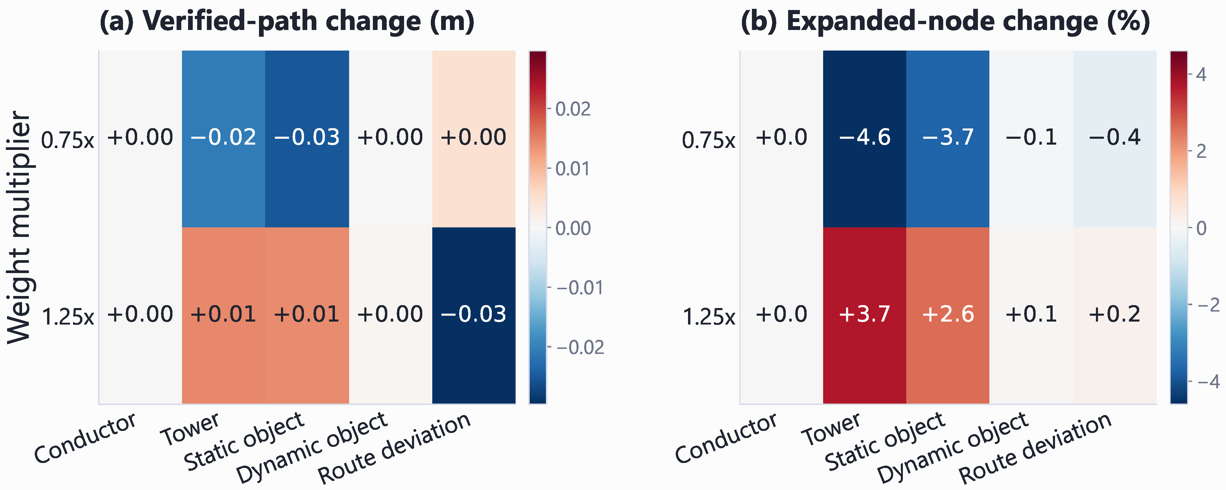
The one-at-a-time experiment perturbs each soft-risk weight by $\pm 25\%$ around the prespecified default while retaining every hard threshold. Across the 4950 trials for all weight conditions, no safety flag was recorded. The largest absolute change in mean verified-path length was 0.03 m, whereas the largest absolute change in the mean number of expanded nodes was 4.6%. Figure 7 therefore distinguishes geometric sensitivity from computational sensitivity rather than reducing the sweep to a single selected weight.

These results support the intended separation of roles. The soft weights alter how admissible alternatives are ranked, while the common verifier continues to decide whether an edge may enter the search or smoothing result. The tested $\pm 25\%$ interval is a local calibration check, not evidence that arbitrary weights are inconsequential.

5.2. Route-Crossing Test of Arrival-Time Prediction

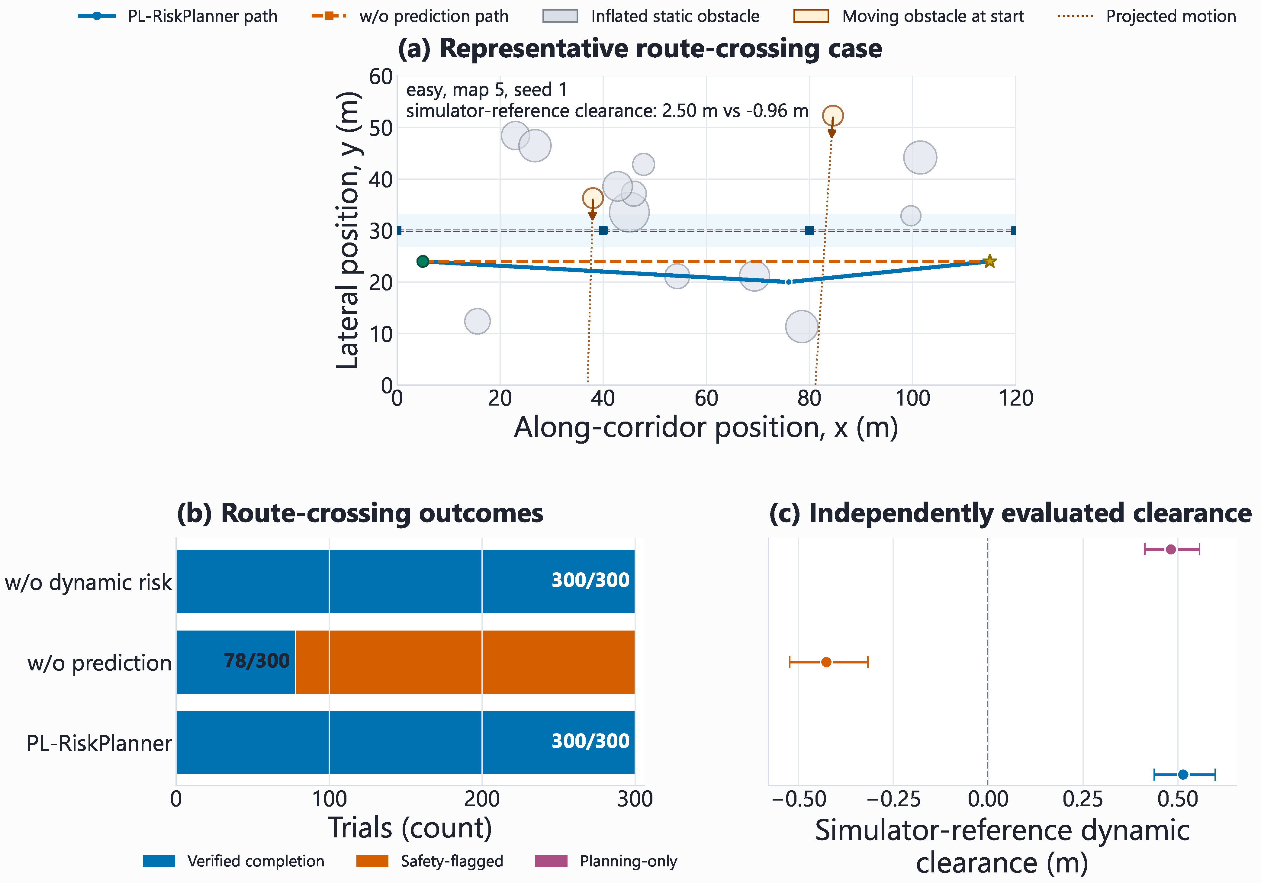
Randomly generated moving objects do not necessarily create a temporal conflict with the nominal route. The route-crossing experiment therefore places moving objects near the route at estimated UAV arrival times and evaluates three matched configurations. Each configuration included 300 trials. For PL-RiskPlanner, no safety flag was recorded. The no-prediction and no-dynamic-risk variants recorded 222 and 0 safety flags, respectively. Mean simulator-reference dynamic clearance over planner-returned paths was 0.51 m, −0.43 m, and 0.48 m, respectively. The no-dynamic-risk variant removes only the soft dynamic-risk term; it retains arrival-time prediction and the corresponding hard admissibility check. The no-prediction variant instead evaluates moving objects at their current positions in both the soft term and the hard check.

Figure 8 links these aggregate counts to a deterministically selected matched case. The selection rule requires a verified PL-RiskPlanner completion and a safety-flagged no-prediction path, prioritizes a collision if present, and then chooses the largest reference-clearance gap. The plotted paths are regenerated from the recorded family, difficulty level, map index, and seed; the regeneration script stops if their path length, clearance, or outcome flags do not match the archived CSV row.

The contrast isolates the timing mechanism more directly than the nominal benchmark. It does not imply that constant-velocity extrapolation resolves all forms of dynamic interaction; acceleration, delayed sensing, and closed-loop tracking remain outside the present simulator.

5.3. Velocity Noise and Uncertainty Margin

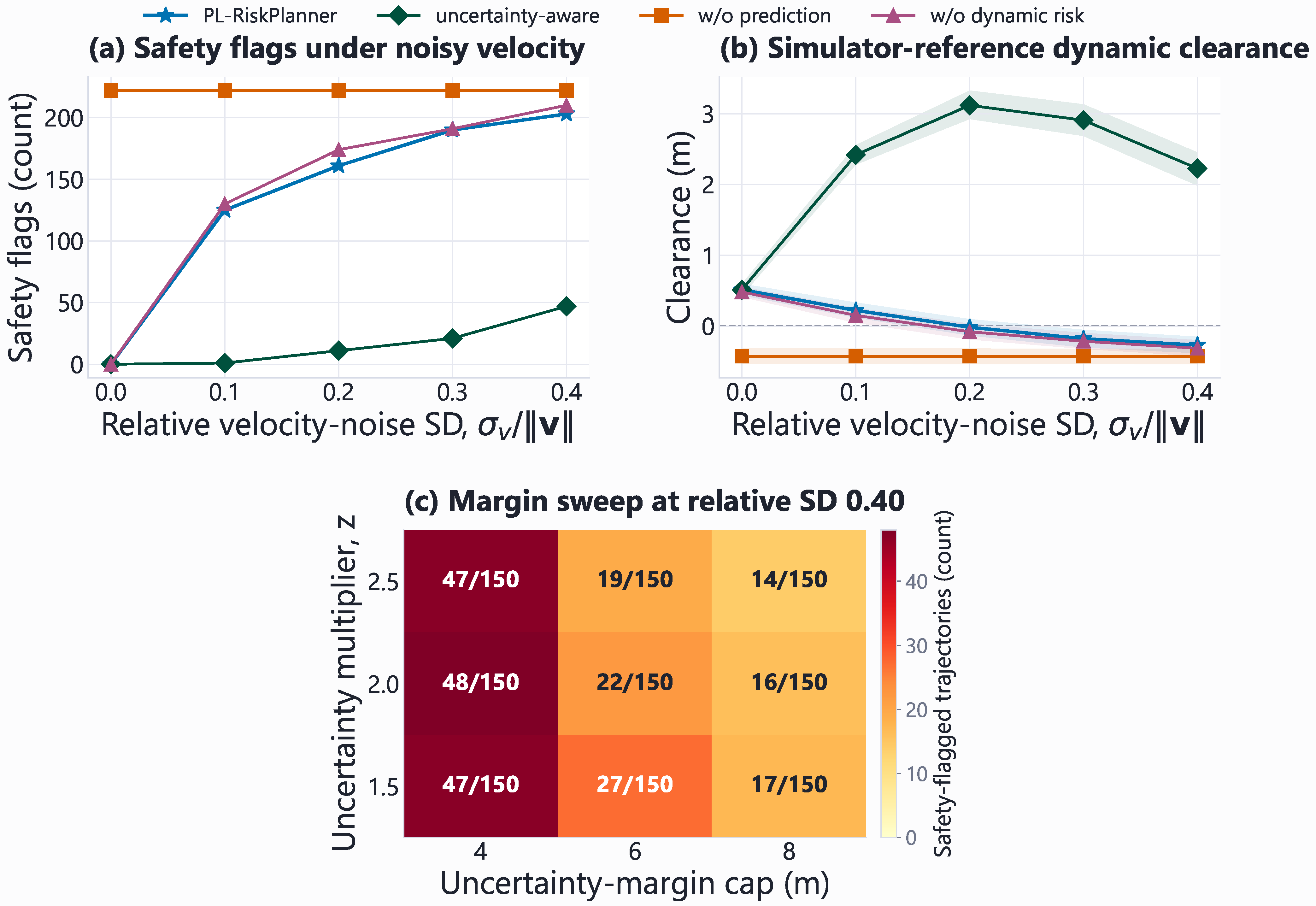
Figure 9 evaluates whether the nominal prediction remains reliable when each perceived velocity component is perturbed while clearance is recomputed from obstacle motion generated with the unperturbed velocity. At the largest tested relative standard deviation, 0.4, each planner configuration included 300 trials. The nominal PL-RiskPlanner recorded 203 safety flags and a mean simulator-reference dynamic clearance of −0.27 m on returned paths. The uncertainty-aware variant recorded 47 flags and 2.23 m clearance under the same noise level.

The uncertainty margin should therefore be interpreted as a robustness trade-off, not a certificate. Larger margins can preserve more separation but also reject candidate edges and increase search effort. Supplementary Tables S7b and S8 retain every noise and margin setting so that the reference $z=2.0$, 6 m cap can be assessed without relying on one plotted cell.

5.4. Scope and Reproducibility

The evidence in Section 4 and Section 5 was generated entirely from synthetic geometry and supplied obstacle states. Its practical value lies in making the planning assumptions and failure accounting inspectable: scenario rules, seeds, parameters, source hashes, raw rows, analysis code, and figure scripts are archived together. It does not validate perception, flight dynamics, wind, communication delay, or real-time replanning on an aircraft.

A subsequent validation program would need to replace the synthetic geometry with surveyed or digital-twin asset models, test realistic timing and sensor streams in a hardware-in-the-loop environment, and then progress through supervised trials in a non-energized mock corridor and, where appropriately authorized, in the field. Those steps are outside the present study and are stated as future requirements rather than completed experiments.

6. Conclusions

We presented PL-RiskPlanner as a safety-constrained, risk-aware planning framework for synthetic power-line corridors. Hard conductor, tower, insulator, static-object, and predicted dynamic-object checks define the sampled feasible set; the power-line risk field ranks only admissible edges; and smoothing reuses the same segment verifier. The methodological claim is therefore constraint consistency across search and postprocessing, not a new or faster A* expansion rule. Across the 1800 nominal matched trials, no safety flag was recorded under the independent sampled evaluation, and the mean verified-path length was 110.64 m. Among matched cases completed by both methods, the mean paired path-length difference (DWA minus PL-RiskPlanner) was 0.16 m (95% bootstrap CI [0.12, 0.2] m); their aggregate verified-path means were 110.8 and 110.64 m, respectively. In addition, disabling verifier-gated smoothing increased mean path length by 13.64 m (95% paired-bootstrap CI [13.37, 13.91] m).

The direct comparison with DWA places this result in context. PL-RiskPlanner’s mean verified path was only 0.160 m shorter in paired trials, while DWA’s mean sampled minimum margin was 0.043 m larger and its mean query time was 2.268 s shorter. In contrast, PL-RiskPlanner returned 25.91 fewer waypoints on average and reduced the lower-is-better smoothness measure by 0.180. It is therefore better positioned here as a compact, globally searched and verifier-gated premission route generator, whereas the tested DWA baseline is a faster local rollout method; neither is claimed to dominate the other on every criterion. The equal-verifier-budget audit further exposed the computational trade-off. Within this cap, PL-RiskPlanner completed 292/450 queries and exhausted the budget in 158, whereas DWA completed 450/450 queries without exhausting the budget. The two planners consumed a mean of 45,577 and 18,696 point checks per query, respectively.

The targeted tests clarify where the dynamic components matter. In 300 route-crossing trials per variant, the no-prediction configuration produced 222 safety flags. For the complete planner, no safety flag was recorded. At the largest tested relative velocity-noise level, the bounded uncertainty margin changed the flag count from 203 to 47 and the mean simulator-reference dynamic clearance on returned paths from −0.27 to 2.23 m. These are condition-specific simulation results rather than a claim of universal or continuous-time safety.

A further contribution is the evaluation record itself: 50,400 trial records, fixed seeds, complete planner parameters, source hashes, controlled clutter factors, ablations, weight perturbations, noise tests, a common hard-verifier-budget audit, and scripts that regenerate the statistics and figures after checking data completeness. The current model does not represent perception, full vehicle dynamics, acceleration of moving objects, or physical flight. Validation with surveyed geometry, realistic timing and sensor streams, hardware-in-the-loop tests, and a staged program of supervised flight trials would therefore be required before drawing conclusions about field operation. The separation between asset-specific distance functions, hard admissibility, and soft guidance also provides an interface for related constrained-planning studies, but transfer beyond power-line corridors remains to be tested.

References

1. Mendu, B.; Mbuli, N. State-of-the-Art Review on the Application of Unmanned Aerial Vehicles (UAVs) in Power Line Inspections: Current Innovations, Trends, and Future Prospects. Drones 2025, 9, 265. [Google Scholar] [CrossRef] [Scilit]
2. Zhang, Y.; Yuan, X.; Fang, Y.; Chen, S. UAV Low Altitude Photogrammetry for Power Line Inspection. ISPRS Int. J. Geo-Inf. 2017, 6, 14. [Google Scholar] [CrossRef] [Scilit]
3. Jalil, B.; Leone, G.R.; Martinelli, M.; Moroni, D.; Pascali, M.A.; Berton, A. Fault Detection in Power Equipment via an Unmanned Aerial System Using Multimodal Data. Sensors 2019, 19, 3014. [Google Scholar] [CrossRef] [Scilit] [PubMed]
4. Li, Y.; Dong, X.; Ding, Q.; Xiong, Y.; Liao, H.; Wang, T. Improved A-STAR Algorithm for Power Line Inspection UAV Path Planning. Energies 2024, 17, 5364. [Google Scholar] [CrossRef] [Scilit]
5. Xing, J.; Cioffi, G.; Hidalgo-Carrió, J.; Scaramuzza, D. Autonomous Power Line Inspection with Drones via Perception-Aware MPC. In Proceedings of the 2023 IEEE/RSJ International Conference on Intelligent Robots and Systems (IROS), Detroit, MI, USA, 1–5 October 2023; pp. 1086–1093. [Google Scholar] [CrossRef] [Scilit]
6. He, Y.; Hou, T.; Wang, M. A New Method for Unmanned Aerial Vehicle Path Planning in Complex Environments. Sci. Rep. 2024, 14, 9257. [Google Scholar] [CrossRef] [Scilit] [PubMed]
7. Zong, Z.; Li, D.; Dong, X.; Cui, Y.; Yang, B.; Xiang, J.; Tu, Z. Risk-Aware Enabled Path Planning for Drones Flight in Unknown Environment. J. Intell. Robot. Syst. 2025, 111, 47. [Google Scholar] [CrossRef] [Scilit]
8. Debnath, D.; Vanegas, F.; Sandino, J.; Hawary, A.F.; Gonzalez, F. A Review of UAV Path-Planning Algorithms and Obstacle Avoidance Methods for Remote Sensing Applications. Remote Sens. 2024, 16, 4019. [Google Scholar] [CrossRef] [Scilit]
9. Meng, W.; Zhang, X.; Zhou, L.; Guo, H.; Hu, X. Advances in UAV Path Planning: A Comprehensive Review of Methods, Challenges, and Future Directions. Drones 2025, 9, 376. [Google Scholar] [CrossRef] [Scilit]
10. Lan, B.; Xing, M.; Lv, H. An Improved Trajectory Generation Algorithm for Outdoor Power Line Inspection. J. Mech. Sci. Technol. 2026, 40, 1403–1415. [Google Scholar] [CrossRef] [Scilit]
11. Hart, P.E.; Nilsson, N.J.; Raphael, B. A Formal Basis for the Heuristic Determination of Minimum Cost Paths. IEEE Trans. Syst. Sci. Cybern. 1968, 4, 100–107. [Google Scholar] [CrossRef] [Scilit]
12. Karaman, S.; Frazzoli, E. Sampling-Based Algorithms for Optimal Motion Planning. Int. J. Robot. Res. 2011, 30, 846–894. [Google Scholar] [CrossRef] [Scilit]
13. Khatib, O. Real-Time Obstacle Avoidance for Manipulators and Mobile Robots. Int. J. Robot. Res. 1986, 5, 90–98. [Google Scholar] [CrossRef] [Scilit]
14. Fox, D.; Burgard, W.; Thrun, S. The Dynamic Window Approach to Collision Avoidance. Robot. Autom. Mag. 1997, 4, 23–33. [Google Scholar] [CrossRef] [Scilit]
15. Kuffner, J.J.; LaValle, S.M. RRT-Connect: An Efficient Approach to Single-Query Path Planning. In Proceedings of the 2000 IEEE International Conference on Robotics and Automation, San Francisco, CA, USA, 24–28 April 2000; Volume 2, pp. 995–1001. [Google Scholar] [CrossRef] [Scilit]
16. Luo, J.; Tian, Y.; Wang, Z. Research on Unmanned Aerial Vehicle Path Planning. Drones 2024, 8, 51. [Google Scholar] [CrossRef] [Scilit]
17. Ait Saadi, A.; Soukane, A.; Meraihi, Y.; Benmessaoud Gabis, A.; Mirjalili, S.; Ramdane-Cherif, A. UAV Path Planning Using Optimization Approaches: A Survey. Arch. Comput. Methods Eng. 2022, 29, 4233–4284. [Google Scholar] [CrossRef] [Scilit]
18. Gao, W.; Li, L.; Pang, D. Urban Low-Altitude UAV Path Planning by Fusing an Enhanced A* Algorithm with an Adaptive Artificial Potential Field Method. Sci. Rep. 2026, 16, 18275. [Google Scholar] [CrossRef] [Scilit] [PubMed]
19. Ahmed, G.; Sheltami, T. Novel Energy-Aware 3D UAV Path Planning and Collision Avoidance Using Receding Horizon and Optimization-Based Control. Drones 2024, 8, 682. [Google Scholar] [CrossRef] [Scilit]
20. Debnath, D.; Hawary, A.F.; Ramdan, M.I.; Vanegas Alvarez, F.; Gonzalez, F. QuickNav: An Effective Collision Avoidance and Path-Planning Algorithm for UAS. Drones 2023, 7, 678. [Google Scholar] [CrossRef] [Scilit]
21. Xie, R.; Meng, Z.; Wang, L.; Li, H.; Wang, K.; Wu, Z. Unmanned Aerial Vehicle Path Planning Algorithm Based on Deep Reinforcement Learning in Large-Scale and Dynamic Environments. IEEE Access 2021, 9, 24884–24900. [Google Scholar] [CrossRef] [Scilit]
22. Zhang, X.; Tan, L.; Chai, J. Direction Aware and Self-Adaptive A* Algorithm with PPO Heuristic for UAV Path Planning of Smart City. Sci. Rep. 2026, 16, 6174. [Google Scholar] [CrossRef] [Scilit] [PubMed]
23. Henderson, P.; Islam, R.; Bachman, P.; Pineau, J.; Precup, D.; Meger, D. Deep Reinforcement Learning That Matters. In Proceedings of the AAAI Conference on Artificial Intelligence, New Orleans, LA, USA, 2–7 February 2018; Volume 32. [Google Scholar] [CrossRef] [Scilit]
24. Tang, H.; Zhu, Q.; Qin, B.; Song, R.; Li, Z. UAV Path Planning Based on Third-Party Risk Modeling. Sci. Rep. 2023, 13, 22259. [Google Scholar] [CrossRef] [Scilit] [PubMed]
25. Braßel, H.; Zeh, T.; Lindner, M.; Fricke, H. Risk-Aware UAV Trajectory Optimization Using Open Urban GIS Data and Target Level of Safety Constraints. Drones 2025, 9, 666. [Google Scholar] [CrossRef] [Scilit]
26. Wang, J.; Zhao, Z.; Qu, J.; Chen, X. APPA-3D: An Autonomous 3D Path Planning Algorithm for UAVs in Unknown Complex Environments. Sci. Rep. 2024, 14, 1231. [Google Scholar] [CrossRef] [Scilit] [PubMed]
27. Xu, L.; Xi, M.; Gao, R.; Ye, Z.; He, Z. Dynamic Path Planning of UAV with Least Inflection Point Based on Adaptive Neighborhood A* Algorithm and Multi-Strategy Fusion. Sci. Rep. 2025, 15, 8563. [Google Scholar] [CrossRef] [Scilit] [PubMed]
28. Zhang, W.; Li, J.; Yu, W.; Ding, P.; Wang, J.; Zhang, X. Algorithm for UAV Path Planning in High Obstacle Density Environments: RFA-Star. Front. Plant Sci. 2024, 15, 1391628. [Google Scholar] [CrossRef] [Scilit] [PubMed]
29. Zhang, Z.; Liu, X.; Feng, B. Research on Obstacle Avoidance Path Planning of UAV in Complex Environments Based on Improved Bézier Curve. Sci. Rep. 2023, 13, 16453. [Google Scholar] [CrossRef] [Scilit] [PubMed]
30. Mellinger, D.; Kumar, V. Minimum Snap Trajectory Generation and Control for Quadrotors. In Proceedings of the 2011 IEEE International Conference on Robotics and Automation, Shanghai, China, 9–13 May 2011; pp. 2520–2525. [Google Scholar] [CrossRef] [Scilit]
Figure 1. Inspection-corridor elements represented in the planning model.
Electronics 15 03676 g001
Figure 2. PL-RiskPlanner workflow and notation. Panel (A) identifies the predecessor, accepted candidate, and rejected candidate; panel (B) distinguishes fixed offline configuration from query-specific computation; panel (C) shows the raw waypoint path, verifier-approved shortcuts, and a rejected edge; and panel (D) gives the corresponding example calculations.
Electronics 15 03676 g002
Figure 3. Representative plan views of the six scenario families at medium difficulty (map index 2, seed 0). Colored circles are inflated spherical-object footprints, black squares are tower axes, and the pale rectangle is the projected conductor safety band. The green circle and orange cross mark the start and goal, respectively. In panel (e), yellow circles and arrows mark moving-object initial positions and velocity directions. Footprints clipped at panel borders extend beyond the plotted workspace boundary and do not represent missing data.
Electronics 15 03676 g003
Figure 4. Matched benchmark. (a) Trial-level outcome accounting; (b) mean path length with 95% bootstrap intervals among verified completions, using the same top-to-bottom planner order as panel (a); (c) mean wall-clock query time with 95% bootstrap intervals over all trials. Counts describe the tested sample and are not interpreted as unconditional probabilities. The colored circular markers in panels (b) and (c) identify the planners listed on the ordinate. No orange segment appears in panel (a) because no safety flag was recorded; the purple segments represent one A*–DWA and 12 RRT* planning-only failures and are narrow on the 1800-trial scale.
Electronics 15 03676 g004
Figure 5. Controlled static-obstacle stress. (a) Verified-completion counts as the target object count changes; (b) verified-path length as obstacle radii are scaled; (c) PL-RiskPlanner wall-clock query time for every count–radius combination. Centers are nested across count conditions, so the plots isolate the controlled burden factors rather than unrelated map draws.
Electronics 15 03676 g005
Figure 6. Component ablation. (a) Outcome accounting for the complete planner and four soft-guidance/postprocessing variants; (b) mean verified-path length with 95% bootstrap intervals in the same top-to-bottom order as panel (a); (c) raw and returned waypoint counts. The no-soft-guidance variant sets λ = 0 but retains the hard verifier; the no-tower-cost variant retains the hard tower clearance, and every smoothing shortcut is rechecked by the common segment verifier. Colored circular markers in panel (b) identify the variants listed on the ordinate. No orange or purple segment appears in panel (a) because all five configurations produced 1800 verified completions and no safety-flagged or planning-only outcome in this benchmark.
Electronics 15 03676 g006
Figure 7. One-at-a-time component-weight sensitivity relative to the default planner. (a) Change in mean verified-path length; (b) percentage change in mean number of expanded nodes. Positive and negative cells indicate increases and decreases relative to the same matched scenarios; hard feasibility is not changed by the perturbation.
Electronics 15 03676 g007
Figure 8. Controlled route-crossing analysis. (a) A matched plan-view case showing the conductor band, inflated static objects, moving-object starts and projected motion, and paths with and without arrival-time prediction; (b) outcome accounting for the three configurations; (c) simulator-reference dynamic clearance on planner-returned paths with 95% bootstrap intervals, using the same top-to-bottom configuration order as panel (b). Clearance in panel (c) is evaluated before safety filtering so that unsafe returned paths remain visible. In panel (a), the green circle and gold star mark the start and goal, respectively; orange circles, arrows, and dotted lines indicate moving-object initial positions, velocity directions, and projected motion. In panels (b,c), blue, orange, and purple identify PL-RiskPlanner, the no-prediction variant, and the no-dynamic-risk variant, respectively. No purple segment appears in panel (b) because no planning-only failure occurred.
Electronics 15 03676 g008
Figure 9. Velocity-noise and uncertainty-margin analysis. (a) Safety-flag counts across five relative velocity-noise levels; (b) mean simulator-reference dynamic clearance on planner-returned paths with 95% bootstrap intervals; (c) safety-flag counts for the z–cap margin sweep at the largest tested noise level. The zero-clearance line in panel (b) distinguishes positive separation from sampled collision.
Electronics 15 03676 g009