Scene-Adaptive Task Offloading in Heterogeneous Edge Networks via Graph Neural Network-Enhanced Deep Reinforcement Learning

Abstract

Efficient task offloading in UAV-assisted heterogeneous mobile edge computing (MEC) networks is increasingly challenged by the co-existence of operationally distinct workload scenarios—including high-demand bursts, resource-constrained periods, and balanced operational states—each demanding fundamentally different assignment strategies. In such networks, mobile executor nodes (e.g., UAVs or vehicle-mounted edge servers) must be dispatched to the vicinity of geographically distributed tasks, making assignment decisions jointly dependent on node mobility, the quality of sensing data, and dynamic resource availability. Conventional approaches based on combinatorial optimization with fixed parameters or greedy heuristics fail to adapt to these varying conditions, leading to resource depletion under sequential workloads or underutilization under high-demand bursts. To address these limitations, this paper proposes SAGE (Scene-Adaptive Graph-Enhanced offloading), a task-offloading framework that combines a heterogeneous graph neural network (HeteroGNN) with a dueling double DQN meta-controller and a mixed-integer linear programming (MILP) solver. At the state-representation level, a heterogeneous bipartite graph is constructed over mobile executor nodes and tasks, with type-specific projection layers encoding the semantic features of each node type and three-dimensional edge features—comprising task success probability, normalized service distance, and link quality—integrated via edge-gated message passing. At the decision level, the meta-controller perceives the current workload scenario through a seven-dimensional situational state vector fused with the graph embedding, selects an appropriate offloading strategy from a learned discrete action space, and drives the MILP solver to perform task-chain assignment under the selected configuration. Experiments on 60 fixed evaluation episodes spanning three representative workload scenarios demonstrate that SAGE achieves an overall reward improvement of 15.9% over the best fixed-strategy baseline, reduces the resource depletion rate to 16.7%, and maintains a high-priority task completion rate of 84.7%. Particularly under resource-constrained conditions, SAGE reduces the reward deficit by 72.3% relative to the best fixed strategy (from $-0.531$ to $-0.147$), demonstrating strong scene-adaptive decision-making capability.

1. Introduction

Driven by the explosive growth of latency-sensitive applications and the proliferation of heterogeneous IoT devices, mobile edge computing (MEC) has emerged as a pivotal paradigm that offloads computation from resource-limited end devices to geographically distributed edge nodes, enabling real-time processing at the network periphery [1,2]. In practical MEC deployments, executor nodes exhibit substantial heterogeneity in computing capacity, communication bandwidth, and task compatibility, while task streams arrive with diverse priority levels, deadline constraints, and resource demands, forming a complex heterogeneous executor-task interaction structure [3,4]. The co-existence of operationally distinct workload conditions—including high-demand task bursts, resource-constrained periods, and stable equilibrium states—further requires that assignment strategies adapt fundamentally to prevailing system states, posing substantial challenges to the intelligent orchestration of heterogeneous edge networks [5,6]. Secure communication and reliable data aggregation have also attracted attention in heterogeneous aerial and satellite-assisted networks, including dynamic group-key agreement for cross-domain heterogeneous data aggregation and authentication mechanisms for UAV flying ad hoc networks [7,8].

Existing approaches to task assignment in heterogeneous MEC environments span combinatorial optimization formulations, heuristic algorithms, and learning-based methods, yet they share a common fundamental limitation: assignment strategies and their associated optimization weights are determined offline and remain fixed throughout deployment, regardless of the prevailing workload scenario [9,10]. While combinatorial optimization methods can yield high-quality solutions under well-specified parameters, their objective coefficients and resource-constraint thresholds are typically hand-tuned for a single workload assumption and cannot be reconfigured in response to dynamic shifts in task arrival rates, node availability, or capacity utilization [1,2]. Heuristic and meta-heuristic algorithms, though computationally efficient, make myopic, greedy decisions that maximize immediate local utility without accounting for cross-task resource coordination or long-term capacity sustainability, leading to node resource depletion under sequential high-demand workloads [6,11]. Reinforcement learning offers strong adaptive potential, yet existing formulations predominantly rely on scalar or low-dimensional state vectors that fail to capture the relational structure between heterogeneous executor nodes and tasks, limiting their effectiveness in multi-node edge environments [12,13].

Motivation. The inability of existing methods to adapt assignment strategies to workload context carries significant operational consequences. Under resource-constrained conditions, scenario-agnostic policies tend to over-commit executor nodes, causing resource depletion and leaving the system unable to handle subsequent task arrivals; conversely, under high-demand bursts, overly conservative policies leave available node capacity underutilized and fail to meet task deadlines [5,11]. As edge systems are increasingly expected to operate autonomously across the full spectrum of workload conditions without manual reconfiguration, the capacity to perceive the system state and dynamically adjust assignment behavior becomes a prerequisite for sustained quality of service rather than an optional enhancement [14,15]. Developing a workload-adaptive task assignment framework that bridges situational awareness and precise resource allocation therefore represents both a pressing engineering need and a meaningful research gap in the intelligent orchestration of heterogeneous edge networks [12].

Challenges. Realizing a scene-adaptive task-offloading framework for heterogeneous edge networks entails three principal technical challenges. First, the bipartite interaction structure between heterogeneous executor nodes and incoming tasks involves two semantically distinct entity types with different feature spaces—including node-computing capacity, link quality, and task resource demand—requiring dedicated relational encoders that go beyond homogeneous graph neural network architectures [12,13]. Second, the system state of a heterogeneous edge deployment is characterized by a high-dimensional, dynamically evolving context vector spanning node utilization, task-queue depth, deadline urgency, and workload intensity, making it non-trivial to extract discriminative scenario features that reliably condition the assignment policy to the current operational regime [5,14]. Third, integrating a learned meta-controller with an MILP solver—wherein the reinforcement learning agent selects problem-formulation parameters that steer the solver toward workload-appropriate solutions—introduces a challenging bi-level optimization structure: the effect of the agent’s strategy selection is mediated through the solver’s deterministic optimization process, creating structural delay between action and reward; moreover, the same strategic action can yield substantially different returns across environmental instances due to varying scene configurations—different task distributions and node states—amplifying reward variance and complicating policy convergence [12,16].

Contributions. To address the above challenges, this work makes the following contributions:

• Heterogeneous Graph-State Representation: We construct a bipartite graph over executor nodes and tasks with type-specific projection layers and edge-gated message passing. Three-dimensional edge features encoding task-success probability, normalized service distance, and link quality are integrated to yield a situationally aware graph embedding that captures the relational structure of the heterogeneous edge network, providing the policy with an expressive representation of executor-task interactions.
• Scene-Adaptive Meta-Controller: We design a dueling double DQN meta-controller that fuses the graph embedding with a seven-dimensional situational state vector to perceive the current workload regime and select among a set of discrete offloading strategies. Each strategy configures the MILP solver with a distinct total assignment budget, chain quality threshold, and deadline-sensitivity weight, enabling the system to adapt its resource allocation behavior to the prevailing workload scenario without manual reconfiguration.
• Principled Action-Space Design via Grid Scanning and Clustering: Rather than manually specifying offloading strategies, we conduct a systematic grid scan over the joint space of assignment budget, chain quality threshold and deadline-sensitivity weight; evaluate each configuration across representative workload scenarios; and apply clustering to identify K behaviorally distinct strategy prototypes. By compressing the continuous parameter space into a compact, discrete action set with well-separated behavioral profiles, this design reduces per-action return variance, sharpens the action–reward correspondence, and thereby alleviates the training difficulty inherent to the bi-level optimization structure.
• Comprehensive Evaluation: We conduct extensive experiments on 60 fixed evaluation episodes spanning three representative workload scenarios. Systematic comparisons with five fixed-strategy baselines, a greedy heuristic, and an end-to-end MAPPO baseline, together with ablation studies, parameter sensitivity analyses, and repeated-run statistical validation with three SAGE training seeds, collectively validate SAGE’s adaptability, resource efficiency, and generalization.

2. Related Work

Task offloading in mobile edge computing is a fundamental research problem involving distributed computing, network resource management, and combinatorial optimization. With the rapid proliferation of resource-constrained IoT devices and latency-sensitive applications, effective offloading mechanisms have become critical for maintaining quality of service in heterogeneous edge environments. Existing approaches can be broadly categorized into two research lines: (i) optimization-based methods, which formulate task offloading as integer programming, convex optimization, or combinatorial optimization problems and seek exact or near-optimal solutions under given system parameters, and (ii) learning-based methods, including deep reinforcement learning, meta-reinforcement learning, multi-agent reinforcement learning, and graph neural network-enhanced approaches, which learn task-offloading policies through interaction with the environment. Although both lines of research have advanced the field in different ways, existing methods still struggle to simultaneously achieve scenario awareness, heterogeneous node representation, constraint feasibility, and multi-round task-service capability in complex heterogeneous environments.

Optimization-based methods. Combinatorial optimization formulations have been widely adopted for MEC task offloading due to their explicit objective functions and constraint representations. Mao et al. [1] proposed a latency-optimal joint task assignment and resource allocation framework for heterogeneous MEC systems. Zhang et al. [2] further considered task dependency constraints and developed a two-stage alternating optimization method to decouple offloading decisions from resource allocation. Kang et al. [17] investigated incentive-aware dependent task offloading from an economic perspective and proposed an iterative combinatorial auction mechanism. Sardellitti et al. [18] jointly optimized radio and computational resources in multicell MEC systems through successive convex approximation. Dinh et al. [16] studied task allocation and computational frequency scaling, using semidefinite relaxation to optimize the trade-off between delay and energy consumption under frequency constraints. Although these methods can obtain high-quality solutions when system parameters are well specified, their objective functions, weighting coefficients, and constraint thresholds are typically predefined, making it difficult to automatically adjust the decision logic in response to changes in task arrivals, node states, and resource availability.

Learning-based methods. Deep reinforcement learning has been widely applied to MEC task offloading because of its ability to learn dynamic offloading policies through environmental interaction. Tang and Wong [3] combined LSTM, dueling DQN, and double DQN to address task offloading in heterogeneous MEC systems. He et al. [6] and Zhao et al. [19] applied multi-agent DRL to D2D MEC and UAV-assisted MEC scenarios, respectively, to model cooperative decision-making among multiple nodes. To improve cross-scenario adaptability, Wang et al. [5] and Li et al. [20] introduced meta-reinforcement learning mechanisms that enable offloading policies to adapt quickly to new environments. Furthermore, GNNs have been employed to enhance topology awareness in edge networks. Sun et al. [12] applied graph reinforcement learning to online computational offloading, Xu et al. [13] proposed TransEdge to capture the spatial correlations of task requests in transportation systems, and Li et al. [21] proposed GASTO to enable fast policy transfer across edge topologies. Shao et al. [22] and Eisen and Ribeiro [23] further demonstrated the generalization capability of GNNs in scalable network resource allocation. Although learning-based methods improve the dynamism and generalization of offloading decisions, most DRL methods still rely on relatively flat state representations, which makes it difficult to fully characterize the relational structure between task nodes and executor nodes. Meanwhile, existing GNN-enhanced methods often lack type-specific modeling for heterogeneous node roles and are rarely integrated with exact combinatorial optimization solvers. As a result, they remain limited in terms of constraint feasibility, decision interpretability, and task-chain-level precise allocation.

As shown in

Table 1. Comparative summary of task-offloading approaches in heterogeneous MEC networks.

Works	Scenario-Aware	Hetero. Nodes	Exact Opt.	Explainable	Multi-Round	Method
Optimization-based methods
Mao [1]	×	✓	✓	✓	×	Opt.
Zhang [2]	×	✓	✓	✓	×	Opt.
Hong [17]	×	×	✓	✓	×	Auction+Opt.
Sardellitti [18]	×	×	✓	✓	×	SCA-Opt.
Dinh [16]	×	✓	✓	✓	×	SDR-Opt.
Learning-based methods
Tang [3]	✓	✓	×	×	×	DRL
He [6]	✓	×	×	×	✓	MARL
Wang [5]	✓	×	×	×	×	Meta-RL
Li [20]	✓	×	×	×	×	Meta-RL
Zhao [19]	✓	✓	×	×	×	MARL
Sun [12]	✓	✓	×	×	×	Graph RL
Xu [13]	✓	✓	×	×	×	GNN+RL
Li [21]	✓	✓	×	×	×	GNN+Meta-RL
Shao [22]	✓	✓	×	×	×	GNN
Eisen [23]	×	×	×	×	×	GNN+RL
Zeng [11]	×	✓	×	×	✓	MARL
Yu [24]	✓	×	×	×	✓	MARL (MAPPO)
Ours	✓	✓	✓	✓	✓	HetGNN+RL+MILP

Note: Opt.: optimization-based method; SCA: successive convex approximation; SDR: semidefinite relaxation; DRL: deep reinforcement learning; MARL: multi-agent reinforcement learning; Meta-RL: meta-reinforcement learning; Graph RL: graph reinforcement learning; Exact Opt.: exact or mathematically grounded optimization solver; Multi-Round: multi-round task execution. ✓ indicates support, and × indicates no support.

, the proposed method integrates type-specific heterogeneous graph representation, high-level learning-based strategy selection, and MILP-based exact task-chain allocation within a unified framework, thereby simultaneously supporting scenario awareness, heterogeneous node modeling, exact optimization, decision interpretability, and multi-round task execution.

3. System Model and Problem Formulation

We study a multi-round task-offloading system in which a heterogeneous UAV-assisted edge network serves a stream of geographically distributed computational tasks arriving with deadlines and priority weights. Executor nodes are modeled as mobile edge computing (MEC) nodes—such as UAVs or vehicle-mounted edge servers—that can be dispatched to the vicinity of tasks, enabling on-site low-latency computation. The objective is to maximize the cumulative weighted task success over a finite episode horizon while managing resource utilization and preventing executor-node depletion.

3.1. Network Architecture

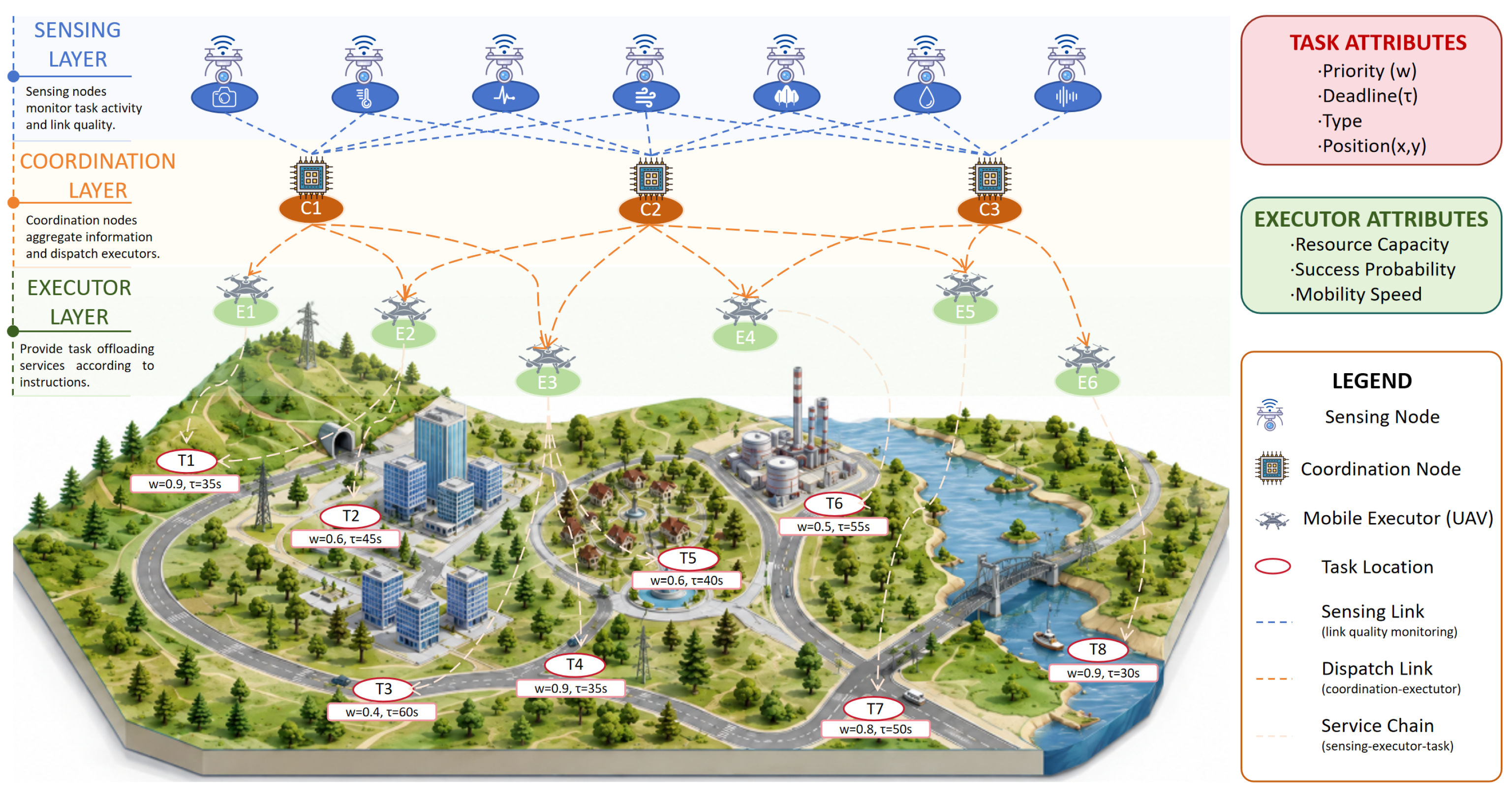
The heterogeneous edge network consists of three types of nodes, as illustrated in Figure 1.

• Sensing nodes ($\mathcal{S}=\{1,\dots ,N_S\}$): Fixed IoT devices or lightweight ground monitoring agents are deployed across the service area. Each sensing node (s) continuously measures the quality of links to reachable executor nodes ($R_{s,i}$), monitors task activity in its vicinity, and forwards task metadata and sensing observations to coordination nodes. The spatial proximity of sensing node s to task j determines the quality of task-related sensing data, which directly influences task execution success probability. $C_{s,j}\in [0,1]$ denotes the observation link quality between sensing node s and task j, modeled analogously to $R_{s,i}$ but over the sensing-to-task channel rather than the sensing-to-executor channel.
• Coordination nodes ($\mathcal{C}=\{1,\dots ,N_C\}$) are ground-based edge controllers that aggregate task information from sensing nodes, maintain task queues, and relay dispatch instructions to executor nodes. The communication relay delay (${\Delta }_{s,i}$) between sensing node s and executor i is incurred through the coordination layer and is incorporated into the feasibility constraint of each service chain.
• Executor nodes ($\mathcal{I}=\{1,\dots ,N_I\}$) are Mobile edge computing nodes (e.g., UAVs or vehicle-mounted servers) that are dispatched to the vicinity of assigned tasks to perform computation on site. Each executor ($i\in \mathcal{I}$) is characterized by remaining resource capacity (${\rho }_i\in [0,{\rho }_i^{\max }]$), a task-type-specific base success probability profile ($P_{i,·}^{\mathrm{base}}$), and maximum flight/travel speed ($v_i$).

Communication between sensing and executor nodes is modeled as a sparse graph ($G=(\mathcal{S}\cup \mathcal{I},\mathcal{E})$). For an edge ($(s,i)\in \mathcal{E}$), the link quality ($R_{s,i})\in [0,1]$ captures channel reliability, and ${\mathrm{Reach}}_{s,i}\in \{0,1\}$ encodes whether sensing node s can reach executor i within its communication range.

3.2. Task Model

Let ${\mathcal{J}}^{\mathrm{pool}}$ denote a global task pool of size $N_{\mathrm{pool}}$. At each round (t), a subset (${\mathcal{J}}_t\subseteq {\mathcal{J}}^{\mathrm{pool}}$) of $|{\mathcal{J}}_t|$ active tasks is available. Each active task ($j\in {\mathcal{J}}_t$) is described by priority weight ($w_j\in (0,1]$), remaining deadline (${\tau }_j\in (0,T_{\max }]$), task type (${\mathrm{type}}_j$), position (${\mathbf{p}}_j\in {\mathbb{R}}^2$), and baseline maximum executor count ($M_j^{\mathrm{base}}$). The system operates for up to $T_{\mathrm{rounds}}$ decision rounds per episode.

3.3. Service-Chain Model

Each assignment decision is a service chain $(s,i,j,k)$, representing a complete execution pathway in which sensing node s provides task monitoring data, and mobile executor i is dispatched to the vicinity of task j at service distance level k (near, mid, far) and performs the computation on site. The $d_k$ parameter denotes the corresponding service-radius threshold.

The task success probability of a service chain captures two independent degradation effects: (i) executor-side degradation, where operating at service distance $d_k$ from the task reduces computation quality due to limited sensing coverage and communication fidelity, and (ii) sensing-side degradation, where a larger spatial separation between sensing node s and task j implies lower quality of task-related observations forwarded to the executor. These are modeled multiplicatively as follows:

$$P_{\mathrm{succ}}(s,i,j,k)=P_{i,{\mathrm{type}}_j}^{\mathrm{base}}·\exp (-\mu ·d_k)·\exp (-\nu ·{\parallel {\mathbf{p}}_s-{\mathbf{p}}_j\parallel }_2),$$

(1)

where $P_{i,{\mathrm{type}}_j}^{\mathrm{base}}$ is the base success rate of executor i for task type ${\mathrm{type}}_j$ and $\mu ,\nu >0$ are distance-decay coefficients. When multiple chains are assigned to task j, their contributions are combined via cooperative probability aggregation:

$${\widehat{P}}_j=1-\prod _{(s,i,j,k)\in {\mathcal{A}}_j}\left(1-P_{\mathrm{succ}}(s,i,j,k)\right).$$

(2)

The flight time for executor i to reach the service radius of task j at level k is $T_{i,j,k}^{\mathrm{fly}}=\max (0,{\parallel {\mathbf{p}}_i-{\mathbf{p}}_j\parallel }_2-d_k)/v_i$, where $v_i$ is the executor’s maximum travel speed. A service chain $(s,i,j,k)$ is feasible only if the total response time satisfies $T_{i,j,k}^{\mathrm{fly}}+{\Delta }_{s,i}\le {\tau }_j$, where ${\Delta }_{s,i}$ is the coordination relay delay between sensing node s and executor i.

3.4. Dynamic Per-Task Executor Limit

To prevent resource over-commitment under constrained conditions, we introduce a dynamic per-task executor limit ($M_j^{\mathrm{eff}}$) that adapts to the current system state. Let $\overline{\rho }={\displaystyle \frac{1}{N_I}}{\sum }_i{\rho }_i/{\rho }_i^{\max }$ be the average resource ratio. The effective limit is

$$M_j^{\mathrm{eff}}=\min \left(M_j^{\mathrm{base}},\mathrm{cap}\left(\overline{\rho }\right)\right),$$

(3)

where

$$\mathrm{cap}\left(\overline{\rho }\right)=\left\{\begin{array}{cc}1\hfill & \overline{\rho }<0.3\hfill \\ 2\hfill & 0.3\le \overline{\rho }<0.6\hfill \\ 3\hfill & \overline{\rho }\ge 0.6\hfill \end{array}\right.,$$

(4)

with the cap increased by one level (up to 3) for high-priority tasks ($w_j\ge 0.65$) or imminent deadlines (${\tau }_j\le 3.0$). The thresholds in Equation (4) partition the normalized average resource ratio into three operating regimes rather than being tuned on the evaluation episodes. When $\overline{\rho }<0.3$, the system is treated as being close to resource depletion, so, at most, one executor is assigned to each task to preserve future service capability. When $0.3\le \overline{\rho }<0.6$, the system has moderate remaining capacity and can support limited cooperation with two executors per task. When $\overline{\rho }\ge 0.6$, the system has sufficient resource headroom, and allowing up to three executors improves the completion probability of urgent or high-priority tasks. This coarse three-level rule also avoids frequent solver reconfiguration caused by small fluctuations in $\overline{\rho }$ while keeping the effect of the dynamic cap interpretable.

3.5. Problem Formulation

The round reward is

$$r_t={\displaystyle \frac{{\sum }_{j\in {\mathcal{J}}_t}{\widehat{P}}_j·w_j}{{\sum }_{j\in {\mathcal{J}}_t}{w}_j}}-\kappa \sum _{j\in {\mathcal{J}}_t^{\exp }}{w}_j-\delta ·\mathbb{1}\left[\mathrm{depletion}\right]·V_{\mathrm{pool}},$$

(5)

where ${\mathcal{J}}_t^{\exp }\subseteq {\mathcal{J}}_t$ is the set of tasks whose deadlines expire in round t without completion; $V_{\mathrm{pool}}={\sum }_{j\in {\mathcal{J}}^{\mathrm{pool}}\setminus {\mathcal{J}}^{\mathrm{seen}}}{w}_j$ is the total priority weight of tasks remaining unspawned in the pool at the moment of resource depletion, serving as an amplifier that makes the depletion penalty proportional to the magnitude of missed opportunity; $\kappa =0.3$ is the per-task deadline-miss coefficient; and $\delta =0.3$ is the resource-depletion coefficient. The value of $\delta =0.3$ is selected to keep the resource-depletion penalty comparable in scale to the deadline-miss penalty while still preserving the normalized task-success term as the primary reward component. In other words, one unit of unserved future task priority caused by complete resource depletion is penalized at the same coefficient level as an expired active task, reflecting the fact that early depletion removes the ability to serve subsequent tasks rather than merely reducing the success probability of the current round. This setting is further examined in the sensitivity analysis in Table 12, where $\delta =0.3$ achieves the lowest depletion rate while retaining competitive overall reward and completion performance. The cumulative objective over an episode is

$$\underset{\pi }{\max }\mathbb{E}\left[{\displaystyle \sum _{t=1}^{T_{\mathrm{rounds}}}}{\gamma }^{t-1}{r}_t\right].$$

(6)

4. Methodology

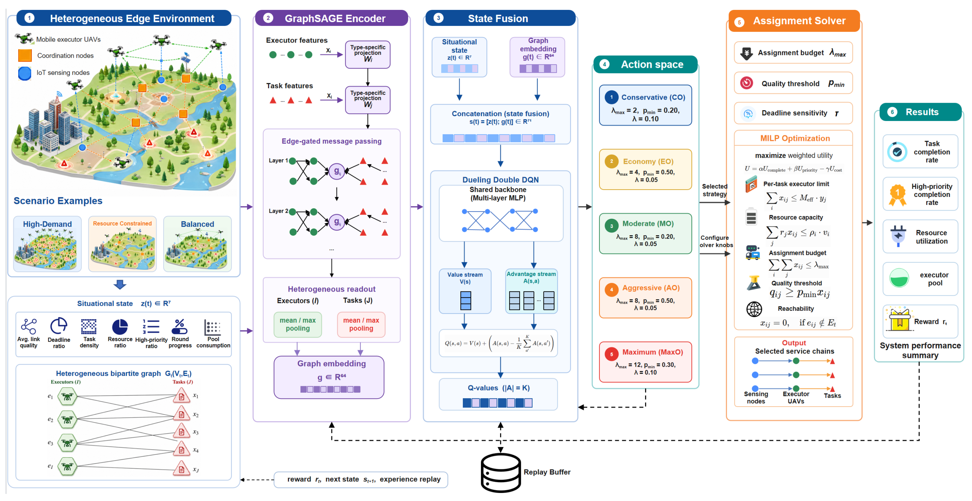
The proposed SAGE framework decouples task offloading into two levels: a meta-controller that perceives the workload scenario and selects an offloading strategy and an MILP solver that executes precise task-chain assignment under the selected configuration. Figure 2 illustrates the overall architecture.

4.1. Heterogeneous Graph-State Representation

4.1.1. Graph Construction

At each decision round (t), we construct a bipartite graph ($G_t=({\mathcal{V}}_t,{\mathcal{E}}_t)$) over executor nodes ($\mathcal{I}$) and active tasks (${\mathcal{J}}_t$). Representing both node types within a unified graph allows the encoder to capture spatial proximity relationships between mobile executors and tasks, directly governing dispatch feasibility and success probability.

Although the MILP decision variable ($x_{s,i,j,k}$) spans a four-tuple (sensing node, executor, task, sand ervice distance level), the GNN graph intentionally omits sensing nodes and service distance levels as explicit vertices. The meta-controller operates at the strategy level and does not need to select individual sensing nodes; instead, sensing-side communication is compactly exposed through an aggregated communication-support feature on each executor-task edge. Specifically, the edge feature includes the maximum reachable sensing-to-executor link quality (${\max }_{s\in \mathcal{S}}{\mathrm{Reach}}_{s,i}{R}_{s,i}$), allowing the controller to observe the communication condition that also appears in the MILP surrogate objective while avoiding an unnecessarily larger tripartite graph. Service distance level (k) is an internal enumeration variable within each service chain and is fully handled by the MILP solver; the meta-controller need not select k explicitly—only the strategy configuration that governs the solver’s feasibility constraints. The GNN therefore captures the relational executor–task structure and the aggregated communication support needed for workload-scenario perception while delegating fine-grained $(s,i,j,k)$ chain selection to the MILP solver—a deliberate separation of responsibilities between the two levels of the bi-level framework.

Node features. Executor node i is represented by ${\mathbf{x}}_i^{\left(I\right)}$, encoding its resource ratio, position, velocity, and capability profile. Task j is represented by ${\mathbf{x}}_j^{\left(J\right)}$, encoding its priority weight, remaining deadline, position, and type.

Edge features. For each feasible pair $(i,j)$, a three-dimensional edge feature vector is constructed, representing the base success probability, normalized service distance, and aggregated sensing-to-executor communication support:

$${\mathbf{e}}_{ij}=\left[P_{i,{\mathrm{type}}_j}^{\mathrm{base}},{\displaystyle \frac{{\parallel {\mathbf{p}}_i-{\mathbf{p}}_j\parallel }_2}{2d_{\max }}},\underset{s\in \mathcal{S}}{\max } {\mathrm{Reach}}_{s,i}{R}_{s,i}\right]\in {\mathbb{R}}^3,$$

(7)

The third component is computed over reachable sensing nodes and exposes the same communication-quality factor ($R_{s,i}$) that influences the MILP objective while still preserving the compact executor–task bipartite graph used by the meta-controller.

4.1.2. Heterogeneous GraphSAGE Encoder

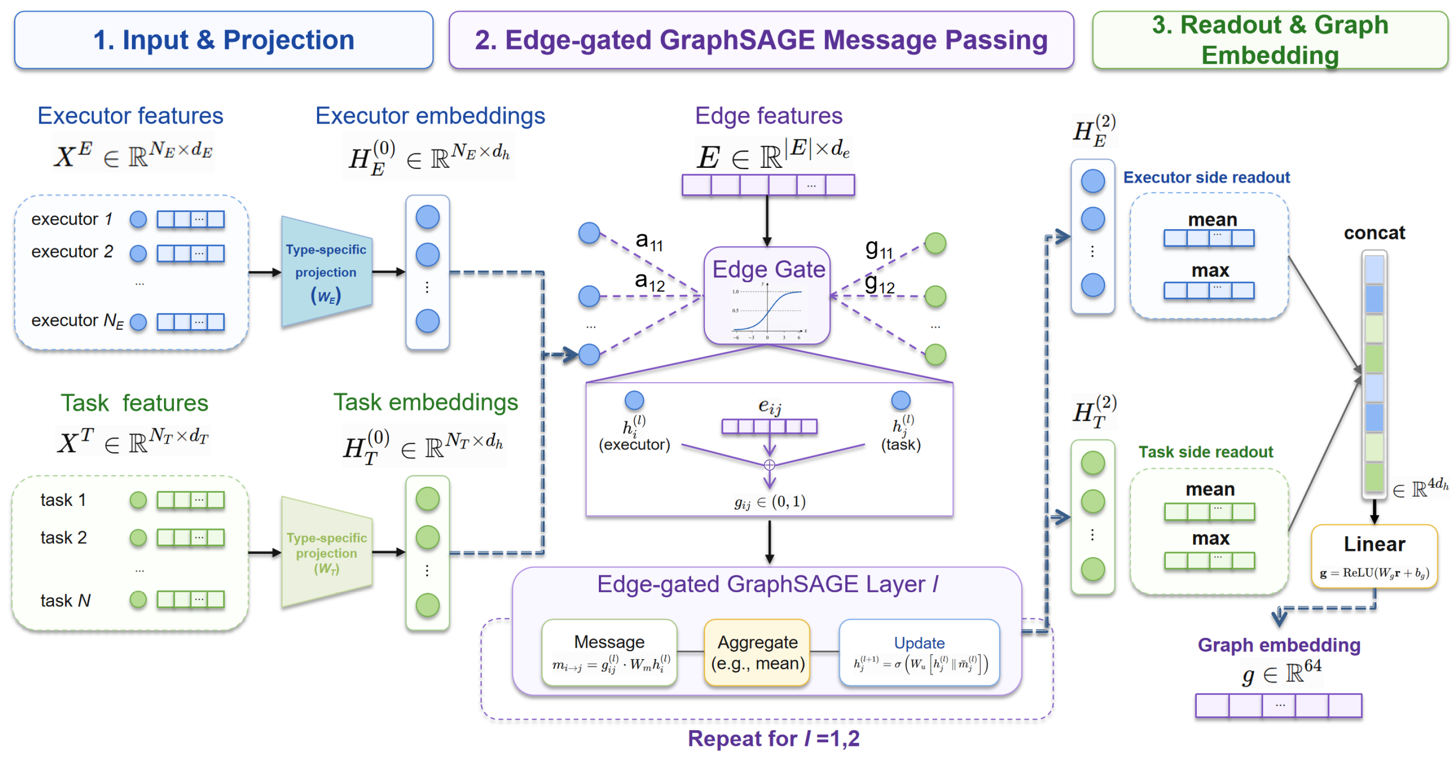
Given the constructed graph, a key challenge is that executor nodes and task nodes carry semantically distinct feature spaces and play fundamentally different roles in the assignment process. A shared graph encoder would conflate these differences. We therefore adopt a Heterogeneous GraphSAGE encoder that applies type-specific input projections before message passing so that each node type is embedded in a meaningful way before neighborhood aggregation begins. The encoder consists of two layers of edge-gated GraphSAGE aggregation (Figure 3).

For reproducibility, the heterogeneous GraphSAGE encoder is implemented as a lightweight PyTorch module without relying on external graph-learning libraries. The executor and task input projections are two independent linear layers with an output dimension of $d_h=64$. Each of the two message-passing layers uses a separate edge-gate layer that maps the three-dimensional edge feature (${\mathbf{e}}_{ij}$) to a scalar gate through a linear transformation followed by a sigmoid activation. The weighted adjacency matrix is obtained by element-wise multiplication of the binary adjacency with the learned edge gate. The aggregated neighbor representation is concatenated with the node’s previous hidden representation, then passed through a linear layer and ReLU activation. After two such layers, executor-side and task-side embeddings are pooled separately using both mean and max pooling, producing four 64-dimensional summary vectors that are concatenated and mapped by a final linear readout layer to the 64-dimensional graph embedding used by the meta-controller. The implementation uses the same padded node order in all batches: executor nodes are placed before active task slots, and inactive task slots are represented by zero features with zero adjacency entries.

Heterogeneous input projection. Executor and task nodes are projected to a shared $d_h=64$-dimensional space via separate linear layers:

$${\mathbf{h}}_i^{\left(0\right)}=\mathrm{ReLU}\left({\mathbf{W}}^{\left(I\right)}{\mathbf{x}}_i^{\left(I\right)}\right),{\mathbf{h}}_j^{\left(0\right)}=\mathrm{ReLU}\left({\mathbf{W}}^{\left(J\right)}{\mathbf{x}}_j^{\left(J\right)}\right),$$

(8)

where ${\mathbf{W}}^{\left(I\right)},{\mathbf{W}}^{\left(J\right)}\in {\mathbb{R}}^{d_h\times d_n}$ are type-specific projection matrices.

Edge-gated message passing. At each layer (ℓ), the edge gate modulates neighbor contributions. A small positive stabilization constant ($ϵ>0$) is included in the normalization denominator to avoid division by zero for isolated or fully gated neighborhoods:

$$\begin{array}{cc}\hfill g_{ij}^{(\ell )}& =\sigma \left({\mathbf{w}}_{\mathrm{gate}}^{(\ell )\top }{\mathbf{e}}_{ij}+b_{\mathrm{gate}}^{(\ell )}\right),\hfill \end{array}$$

(9)

$$\begin{array}{cc}\hfill {\mathbf{m}}_v^{(\ell )}& ={\displaystyle \frac{{\sum }_{u\in \mathcal{N}\left(v\right)}{A}_{uv}{g}_{uv}^{(\ell )}{\mathbf{h}}_u^{(\ell -1)}}{{\sum }_u{A}_{uv}{g}_{uv}^{(\ell )}+ϵ}},\hfill \end{array}$$

(10)

$$\begin{array}{cc}\hfill {\mathbf{h}}_v^{(\ell )}& =\mathrm{ReLU}\left({\mathbf{W}}_{\mathrm{conv}}^{(\ell )}\left[{\mathbf{h}}_v^{(\ell -1)}\parallel {\mathbf{m}}_v^{(\ell )}\right]\right),\hfill \end{array}$$

(11)

where $\sigma$ is sigmoid, $A_{uv}$ is the bipartite adjacency, and $\parallel ·\parallel$ denotes concatenation.

Heterogeneous readout. The graph embedding is obtained by separately pooling executor and task sides:

$$\mathbf{g}={\mathbf{W}}_{\mathrm{out}}\left[\mathrm{mean}\left({\mathbf{H}}^{\left(I\right)}\right)\parallel \max \left({\mathbf{H}}^{\left(I\right)}\right)\parallel \mathrm{mean}\left({\mathbf{H}}^{\left(J\right)}\right)\parallel \max \left({\mathbf{H}}^{\left(J\right)}\right)\right]\in {\mathbb{R}}^{64}.$$

(12)

4.2. Situational State Vector

To complement the graph embedding with global workload context, we construct a seven-dimensional state vector:

$$\mathbf{z}\left(t\right)=\left[z_0,\dots ,z_6\right]\in {\mathbb{R}}^7,$$

(13)

where $z_0$ is the average link quality, $z_1$ is the average remaining deadline ratio ($\overline{\tau }/T_{\max }$), $z_2$ is the active task density, $z_3$ is the average executor resource ratio ($\overline{\rho }$), $z_4$ is the high-priority task ratio, $z_5$ represents round progress ($t/T_{\mathrm{rounds}}$), and $z_6$ is the task-pool consumption ratio. The full state fed to the Q-network is $\mathbf{s}\left(t\right)=[\mathbf{z}\left(t\right)\parallel \mathbf{g}\left(t\right)]\in {\mathbb{R}}^{71}$. This fused representation enables the meta-controller to condition strategy selection on both the local executor-task interaction structure captured by the graph and the global workload context captured by the situational vector.

4.3. Scene-Adaptive Meta-Controller

4.3.1. Action Space

The meta-controller selects from $K=5$ discrete offloading strategies, each specifying a configuration that directly parameterizes the MILP solver via three control variables: the total assignment budget (${\Lambda }^{\max }$), the chain quality threshold ($p_{\min }$), and the deadline sensitivity weight ($\lambda$) on the latency-risk penalty in the objective function.

Action-space design via grid scanning and clustering. Rather than hand-tuning strategy configurations, we derive the action set through a data-driven procedure. We generate episodes from three representative workload scenario types: high-demand (dense, high-priority tasks and ample executor resources), resource-constrained (low executor resource availability), and balanced (moderate task density and resource levels). For each episode, we exhaustively evaluate all parameter combinations over a discrete grid, i.e., ${\Lambda }^{\max }\in \{2,4,6,8,10,12\}$, $p_{\min }\in \{0.2,0.3,0.4,0.5,0.6\}$, and $\lambda \in \{0.0,0.05,0.10,0.15,0.20\}$, yielding 150 candidate configurations, and record the best-performing configuration for that episode. The resulting set of per-episode best-configuration vectors is then clustered using K-means with $K=5$ into behaviorally distinct prototypes, and each cluster center is snapped to the nearest grid point to obtain the final action set. This procedure ensures that the five actions collectively cover the full spectrum of workload conditions, with well-separated behavioral profiles that reduce per-action return variance and sharpen the action-reward signal during policy learning. The resulting five strategy configurations are shown in

Table 2. Discrete offloading strategy configurations.

ID	Name	Max Assign.	${\mathit{p}}_{\min }$	$\mathit{\lambda }$	Intended Scenario
0	Conservative (CO)	2	0.20	0.10	Severe resource shortage
1	Economy (EO)	4	0.50	0.05	Moderate resource constraint
2	Moderate (MO)	8	0.20	0.05	Balanced, broad coverage
3	Aggressive (AO)	8	0.50	0.05	High demand, quality-focused
4	Maximum (MaxO)	12	0.30	0.10	High demand, full deployment

.

To avoid information leakage, the episodes used for action-space construction are generated independently from the episodes used for DQN training and final evaluation. The prototype-building set shares only the scenario-family definitions with the training and evaluation sets while using disjoint random seeds and no overlapping episode instances.

4.3.2. Dueling Double DQN

The Q-network adopts the dueling DQN architecture [25], decomposing the action-value function into state-value and advantage streams:

$$Q(\mathbf{s},a;\mathit{\theta })=V(\mathbf{s};{\mathit{\theta }}_V)+A(\mathbf{s},a;{\mathit{\theta }}_A)-{\displaystyle \frac{1}{K}}\sum _{a^{\prime }}A(\mathbf{s},a^{\prime };{\mathit{\theta }}_A),$$

(14)

where V and A are two-layer MLPs (hidden dimension of 256) sharing feature extraction layers. The double DQN target [26] decouples action selection from value estimation:

$$y_t=r_t+\gamma ·Q\left({\mathbf{s}}_{t+1},\arg \underset{a^{\prime }}{\max }Q({\mathbf{s}}_{t+1},a^{\prime };\mathit{\theta });{\mathit{\theta }}^{-}\right),$$

(15)

where ${\mathit{\theta }}^{-}$ are the parameters of the target network, updated every 20 episodes. Once action $a_t$ is selected, it configures the MILP solver by instantiating ${\Lambda }^{\max }$, $p_{\min }$, and $\lambda$ according to Table 2, which then determines the service-chain assignments for round t.

4.4. MILP-Based Task Assignment Solver

Given the action configuration selected by the meta-controller, the MILP solver computes the optimal task-chain assignment. The decision variable ($x_{s,i,j,k}\in \{0,1\}$) indicates whether service chain $(s,i,j,k)$ is selected. The solver maximizes a weighted utility that balances task success against deadline risk:

$$\underset{\mathbf{x}}{\max }\sum _{(s,i,j,k)}{x}_{s,i,j,k}\left[w_j·R_{s,i}·P_{\mathrm{succ}}(s,i,j,k)-\lambda ·\mathrm{Esc}(s,i,j,k)\right],$$

(16)

where $\mathrm{Esc}(s,i,j,k)=\min \left(\max \left(0,{\displaystyle \frac{T_{i,j,k}^{\mathrm{fly}}+{\Delta }_{s,i}}{{\tau }_j}}\right),1\right)$ is the normalized latency risk of chain $(s,i,j,k)$ and $\lambda$ is the deadline sensitivity weight set by the selected action, subject to the following:

$$\begin{array}{cc}\hfill \sum _{s,k}{x}_{s,i,j,k}& \le 1,\forall i,j,\hfill \end{array}$$

(17)

$$\begin{array}{cc}\hfill \sum _{s,j,k}{x}_{s,i,j,k}& \le 1,\forall i,\hfill \end{array}$$

(18)

$$\begin{array}{cc}\hfill \sum _{s,i,k}{x}_{s,i,j,k}& \le M_j^{\mathrm{eff}},\forall j,\hfill \end{array}$$

(19)

$$\begin{array}{cc}\hfill \sum _{s,j,k}{x}_{s,i,j,k}·r_{i,k}& \le {\rho }_i,\forall i,\hfill \end{array}$$

(20)

$$\begin{array}{cc}\hfill \sum _{s,i,j,k}{x}_{s,i,j,k}& \le {\Lambda }^{\max },\hfill \end{array}$$

(21)

$$\begin{array}{cc}\hfill P_{\mathrm{succ}}(s,i,j,k)·x_{s,i,j,k}& \ge p_{\min }·x_{s,i,j,k},\forall s,i,j,k,\hfill \end{array}$$

(22)

$$\begin{array}{cc}\hfill x_{s,i,j,k}& \le {\mathrm{Reach}}_{s,i},\forall s,i,j,k.\hfill \end{array}$$

(23)

The first newly added constraint ensures that, for any executor–task pair, at most, one service chain can be selected across different sensing nodes and service distance levels. The second, newly added constraint further enforces the physical scheduling assumption that each mobile executor can serve, at most, one task in a decision round, preventing one executor from being assigned to multiple spatially separated tasks simultaneously. Constraints (19) and (20) enforce per-task executor limits and per-executor resource capacity. Constraint (21) bounds the total assignment count. Constraint (22) filters chains with insufficient success probability. Constraint (23) ensures reachability.

Remark (surrogate objective). The MILP objective (16) is a linear surrogate for the round reward (5). The true reward aggregates per-task cooperative success probability (${\widehat{P}}_j$) via a nonlinear multi-chain combination, which would render the MILP non-convex and computationally intractable. The surrogate replaces ${\widehat{P}}_j$ with a chain-level linear term ($w_j·R_{s,i}·P_{\mathrm{succ}}(s,i,j,k)$), preserving the qualitative incentive structure—higher-quality, higher-priority chains are preferred—while keeping the formulation MILP-tractable for branch-and-bound solvers. The gap between surrogate and true reward is absorbed by the meta-controller: because the DQN is trained end-to-end on the actual environmental reward ($r_t$), it implicitly learns to select strategies whose solver solutions yield high true reward, even though the solver itself optimizes only the surrogate.

Small-instance surrogate fidelity check. To quantify the mismatch between the linear surrogate and the nonlinear true reward, we conducted an exhaustive enumeration check on randomly generated small instances that preserve the structural scale of each decision round: 8 sensing nodes, 12 executor nodes, 5–8 active tasks, and 5 service distance levels. For each assignment budget (${\Lambda }^{\max }\in \{4,8,12\}$), 1000 valid instances were generated. All feasible assignments satisfying executor exclusivity and task-capacity constraints were enumerated, and the assignment selected by the linear surrogate was compared with the assignment that maximizes the nonlinear true reward based on cooperative success aggregation. The surrogate does not always select the identical true-reward-optimal assignment, but the true-reward loss remains small, on average, as summarized below (

Table 3. Small-instance surrogate fidelity between the MILP surrogate and nonlinear true reward.

${\Lambda }^{\max }$	Same Assign.	Lower True Reward	Avg. Rel. Gap	Max Rel. Gap
4	40.9%	59.1%	4.57%	26.95%
8	47.0%	53.0%	2.37%	20.86%
12	49.7%	50.3%	2.05%	20.86%

).

These results show that the surrogate may choose a different assignment in roughly half of the enumerated instances, but the average relative true-reward gap remains limited to 2.05–4.57%. Thus, the surrogate should be interpreted as a tractable approximation rather than an exact reformulation of the nonlinear reward; nevertheless, under the assignment constraints used in this work, its empirical fidelity is sufficient to provide reliable solver feedback to the meta-controller.

The solver is implemented using PySCIPOpt with a 3.0 s time limit per round; given the problem scale (at most, 12 executor nodes, 45 task slots, and 5 service distance levels), SCIP consistently reaches a near-zero optimality gap well within this budget in practice, and the time limit serves as a safeguard against pathological instances rather than a binding constraint. The MILP solution determines which service chains are executed; the environment then computes the round reward ($r_t$) and advances to state ${\mathbf{s}}_{t+1}$, completing one step of the bi-level interaction loop. The meta-controller is trained on the resulting transitions as described below.

4.5. Training Procedure

The meta-controller is trained via experience replay and $\epsilon$-greedy exploration. Key hyperparameters: learning rate of $\eta =3\times {10}^{-4}$, discount factor of $\gamma =0.95$, batch size of $B=256$, replay buffer size of 50,000, minimum buffer before training of 1000, exploration decay over 1500 steps ($\epsilon$: $1.0\to 0.05$), and 8000 total training episodes. At each round, the agent observes state ${\mathbf{s}}_t$, selects action $a_t$, drives the MILP solver, receives reward $r_t$, stores the transition $(s_t,a_t,r_t,s_{t+1})$, and updates the Q-network via mini-batch gradient descent on the double DQN loss.

5. Simulation and Results

This section evaluates the proposed framework from three complementary perspectives: overall performance against baselines, ablation analysis of key architectural components, and sensitivity to critical design parameters. Under a shared evaluation protocol consisting of 60 fixed episodes spanning three representative workload scenarios, the proposed SAGE method is compared against five fixed offloading strategies, a greedy heuristic, and an end-to-end MAPPO baseline, assessing its adaptability across varying workload conditions and its advantage over both non-adaptive and learning-based alternatives. Ablation experiments are then conducted to quantify the individual contributions of edge-gated graph encoding, heterogeneous node projection, and the dynamic per-task executor limit. Sensitivity analyses examine how the depletion penalty coefficient ($\delta$) and the number of discrete actions (K) affect reward and resource efficiency, identifying robust operating points.

5.1. Experimental Setup

Evaluation protocol. All methods are evaluated on a fixed set of 60 episodes generated prior to any training, comprising 20 episodes each from three representative workload scenarios: High-Demand (HD), Resource-Constrained (RC), and Balanced (BL). These 60 held-out episodes are used exclusively for final performance comparison and are not involved in action-space construction, DQN training, hyperparameter selection, or model checkpoint selection. Fixed evaluation scenes eliminate sampling noise and ensure fair comparison.

Workload scenarios. Three scenario types are defined by distinct parameter ranges governing task density, resource availability, and task priority composition, as summarized in

Table 4. Quantitative parameter ranges for the three evaluation scenarios.

Parameter	High-Demand (HD)	Resource-Constrained (RC)	Balanced (BL)
Link quality ($R_{\mathrm{scale}}$)	0.70–1.00	0.70–1.00	0.75–1.00
Graph density	0.40–0.70	0.40–0.70	0.50–0.80
Resource ratio ($\rho$ )	0.70–1.00	0.10–0.35	0.70–1.00
Task count (n)	36–45	24–45	18–36
High-priority ratio	0.65–1.00	0.20–0.50	0.20–0.50

. (1) High-Demand (HD): The largest task pool (36–45 tasks), with a high proportion of high-priority tasks ($w_j$ ratio: 0.65–1.0) and ample executor resources ($\rho$: 0.7–1.0), stressing assignment throughput. (2) Resource-Constrained (RC): Executor nodes begin with severely limited resources ($\rho$: 0.1–0.35), the defining characteristic that distinguishes this scenario and creates strong pressure for conservative strategy selection. (3) Balanced (BL): Moderate task count (18–36), intermediate priority composition (0.2–0.5), and sufficient resources ($\rho$: 0.7–1.0), representing the nominal operating condition.

Workload generation and fixed simulation parameters. To improve reproducibility,

Table 5. Fixed simulation and workload-generation parameters.

Item	Setting
Network size and coordinates	8 sensing nodes, 12 mobile executor nodes, and 5 coordination nodes; all node and task coordinates are uniformly sampled in a $100\times 100$ two-dimensional region.
Episode horizon and resources	Each episode lasts at most 8 decision rounds. Executor resources are consumed irreversibly, with no resource replenishment during an episode. Each selected service chain consumes one resource unit.
Task process	The task-pool size follows the scenario-specific task count in Table 4. Initially, 5–8 tasks are active. When the active-task count falls below 5, waiting tasks are sequentially activated until the active set is restored to a randomly sampled size between 5 and 8 or the waiting pool is exhausted.
Task attributes	Tasks are categorized into five service classes represented by one-hot type labels; two latency-critical classes are treated as high-priority tasks. The service tolerance (${\tau }_j$) is sampled from $U(3,6)$, the maximum number of executors per task is sampled from $\{1,2,3\}$, and the task resource cost is 1.0.
Deadline and mobility	The remaining lifetime ($t_j^{\mathrm{remain}}$) is sampled from $U(4,12)$ for high-priority tasks and from $U(12,30)$ for other tasks. Task mobility speeds are sampled from $U(1.5,3.5)$ and $U(0.5,2.0)$ for high-priority and other tasks, respectively, with a uniformly sampled movement direction and boundary reflection.
Executor attributes	Executor types are uniformly assigned among heavy, light, and intercept nodes. Their speed/resource ranges are 15–25/6–12, 25–40/6–9, and 40–60/3–6, respectively.
Communication layer	A sparse communication graph is generated with the graph-density range in Table 4. Sensing–executor pairs under different coordination nodes are unreachable. For reachable pairs, link quality is computed from shortest-path hops with small Gaussian noise, then scaled by $R_{\mathrm{scale}}$; communication delay is $0.01$ times the hop count.
Success and penalty coefficients	The success-probability decay coefficients are $\mu =0.1$ and $\nu =0.005$. The deadline-miss and resource-depletion penalty coefficients are both set to 0.3.

reports the fixed simulation parameters and workload-generation rules used across all training and evaluation episodes. All random variables are sampled independently under the seed assigned to each episode.

The workload generator follows a deterministic seed-controlled pipeline. For each episode, the scenario label first determines the sampling intervals reported in the scenario-parameter table. The episode seed is then used to sample the graph density, communication-quality scale, executor resource ratio, total task-pool size, and high-priority ratio. Based on these sampled values, the generator creates the sensing nodes, mobile executor nodes, coordination nodes, sparse communication topology, and task pool. The task pool is maintained as a sequential workload: only 5–8 tasks are active at initialization, and after each decision round, new waiting tasks are activated whenever the active set falls below five. The same episode seed also fixes task mobility, deadline countdown, stochastic task-success realization, and resource-consumption evolution within the simulation. For the final evaluation, 20 seeds per scenario are materialized before training and reused unchanged by all compared methods.

Software, hardware, and statistical settings. 

Table 6. Software, hardware, and training/statistical configuration.

Item	Setting
Runtime environment	Windows 10; Python 3.11.7; PyTorch 2.3.1; PySCIPOpt 5.4.1 with SCIP.
Hardware	NVIDIA GeForce RTX 2060 GPU; AMD64 Family 23 Model 96 CPU; 15.87 GB RAM.
SAGE training	Dueling Double DQN; 8000 training episodes; Adam optimizer; learning rate of $3\times {10}^{-4}$; batch size of 256; discount factor of 0.95; replay buffer of 50,000; minimum replay size of 1000; target-network update every 20 episodes.
Exploration and seeds	$\epsilon$-greedy exploration decays from 1.0 to 0.05 over 1500 steps. SAGE repeated-run training seeds are 24, 25, and 26. The original held-out evaluation seeds are 20–79, with 20 episodes per scenario.
Baselines	Fixed and greedy strategies have no trainable parameters and are evaluated deterministically on the same held-out episodes. MAPPO is trained for 5000 episodes with seed 42, a learning rate of $3\times {10}^{-4}$, discount factor of 0.95, PPO clip of 0.2, entropy coefficient of 0.01, GAE parameter of 0.95, value-loss coefficient of 0.5, four PPO update epochs and 0.5 gradient clipping.
Statistical protocol	95% confidence intervals use the Student t distribution. Significance is tested with paired t-tests using scenario and episode seeds as the pairing key; for SAGE, the three training seeds are averaged per evaluation episode before paired comparison.

summarizes the implementation environment, training configuration, and statistical protocol used for the learning-based models and baselines. Fixed-strategy baselines and the greedy heuristic are deterministic once the evaluation episode is fixed; therefore, they do not involve optimizer, batch-size, or training-seed settings. For SAGE, repeated-run validation is conducted with three independently trained dueling double DQN models. MAPPO is evaluated from the available trained checkpoint on the same held-out episodes, and this single-checkpoint limitation is explicitly considered when interpreting the MAPPO comparison.

5.2. Evaluation Metrics

Six metrics are reported: (i) overall reward (primary; Equation (5)), the normalized cumulative weighted task success minus deadline-miss and depletion penalties; (ii) the task completion rate, the fraction of all activated tasks successfully completed within their deadlines; (iii) the high-priority completion rate, the completion rate restricted to tasks with high priority weights ($w_j\ge 0.65$); (iv) Resource Utilization, the fraction of total executor node resources consumed across the episode; (v) the resource depletion rate, the fraction of episodes in which all executor resources are exhausted before the episode horizon; and (vi) the mean $P_{\mathrm{succ}}$, the average per-assignment task success probability (Equation (1)) over all service chains executed in an episode, reflecting the quality of individual offloading decisions independently of resource consumption.

5.3. Baseline Methods

Seven baselines spanning three categories are evaluated. Fixed-strategy baselines (1–5). Each baseline corresponds to one of the five discrete offloading strategies in Table 2 and applies that strategy uniformly across all decision rounds, regardless of the current workload scenario. Conservative (CO) uses the smallest assignment budget (${\Lambda }^{\max }=2$) and is designed for severe resource shortage, Economy (EO) sets ${\Lambda }^{\max }=4$ with a strict quality threshold ($p_{\min }=0.5$) for moderate constraints, Moderate (MO) allows up to eight assignments with a relaxed threshold to maximize coverage under balanced conditions, Aggressive (AO) combines ${\Lambda }^{\max }=8$ with the strict threshold to prioritize quality under high demand, and Maximum (MaxO) deploys the full budget (${\Lambda }^{\max }=12$) for intensive workloads. These baselines collectively test whether a single fixed configuration can match the performance of scene-adaptive selection across all scenarios.

Greedy heuristic. At each round, all feasible service chains are enumerated and ranked in descending order of $P_{\mathrm{succ}}(s,i,j,k)\times w_j$; chains are greedily selected in this order until each executor’s resource capacity is exhausted or no feasible chains remain. Unlike the MILP solver, the greedy approach makes no attempt at global resource coordination or per-task executor-count control, serving as a strong non-learning baseline that validates the necessity of exact combinatorial optimization.

End-to-end MAPPO. In a multi-agent proximal policy optimization baseline [24,27] in which each of the 12 executor nodes acts as an independent agent, each agent observes a 231-dimensional local observation (own resource state plus features of all task slots) and selects one of 46 discrete actions (idle or offload to one of 45 task slots) with action masking to suppress infeasible choices. A centralized critic conditioned on the 79-dimensional global state is used during training (CTDE paradigm), while execution is fully decentralized. This baseline directly compares end-to-end multi-agent RL against the proposed two-level meta-controller plus MILP-solver architecture, isolating the contribution of the MILP solver for global resource-constrained assignment.

MAPPO implementation details. For reproducibility, the MAPPO baseline is trained for 5000 episodes, with each episode lasting, at most, eight decision rounds and containing 12 executor agents. Each episode produces one trajectory, followed by four PPO update epochs. Curriculum learning is used during training: the balanced and high-demand scenarios are used in the first 2000 episodes, and the resource-constrained scenario is introduced from episode 2001. The learning rate is 3 $\times {10}^{-4}$, the discount factor is 0.95, the PPO clipping coefficient is 0.2, the entropy coefficient is 0.01, the generalized advantage estimation parameter is 0.95, the value-loss coefficient is 0.5, the gradient-clipping threshold is 0.5, and the training seed is 42. Actor parameters are shared by executor type, yielding three actor networks for heavy, light, and intercept executors, each with a 231-128-128-46 multilayer perceptron; the centralized critic uses a 79-256-256-1 multilayer perceptron. The total parameter counts are 156,426 for the actors and 86,529 for the critic. The action mask keeps no-op always feasible and permits task-slot actions only when the executor is available and has at least one remaining resource unit and the task is active; logits of infeasible actions are set to a large negative value before sampling. Training uses masked categorical sampling, whereas evaluation uses deterministic argmax from the final checkpoint. Unlike SAGE, MAPPO does not call the SCIP-based MILP solver; instead, agents directly select task slots, and the environment retains the highest-success assignments up to each task’s executor limit. It is therefore used as a decentralized multi-agent baseline under the same scenario generator, episode horizon, and penalty definitions rather than as a solver-assisted counterpart to SAGE.

5.4. Comparison with Baseline Methods

5.4.1. Overall Performance

Table 7. Overall performance comparison across 60 evaluation episodes (mean ± std).

Method	Reward	Compl. Rate	HP Compl.	Res. Util.	Depl. Rate	Mean ${\mathit{P}}_{\mathbf{succ}}$
SAGE (Ours)	2.878 ± 2.637	76.3% ± 20.4%	84.7% ± 20.6%	71.7% ± 15.3%	16.7% ± 37.6%	0.488 ± 0.071
CO (max = 2)	0.845 ± 1.894	56.8% ± 10.4%	69.9% ± 21.1%	33.7% ± 18.4%	18.3% ± 39.0%	0.569 ± 0.049
EO (max = 4)	1.773 ± 2.199	67.5% ± 16.3%	79.9% ± 22.4%	49.5% ± 12.9%	21.7% ± 41.5%	0.533 ± 0.039
MO (max = 8)	2.165 ± 3.101	74.7% ± 21.1%	84.0% ± 21.3%	72.2% ± 14.1%	40.0% ± 49.4%	0.461 ± 0.052
AO (max = 8)	2.484 ± 2.739	74.8% ± 20.9%	82.3% ± 21.5%	66.6% ± 12.2%	25.0% ± 43.7%	0.488 ± 0.047
MaxO (max = 12)	2.179 ± 3.163	74.9% ± 21.5%	83.4% ± 22.6%	75.7% ± 15.5%	43.3% ± 50.0%	0.443 ± 0.051
Greedy	1.867 ± 3.187	72.2% ± 22.4%	81.3% ± 24.0%	76.9% ± 15.4%	50.0% ± 50.4%	0.385 ± 0.042
MAPPO	0.722 ± 2.432	59.8% ± 15.5%	70.2% ± 23.5%	57.4% ± 13.5%	31.7% ± 46.9%	0.334 ± 0.044

presents performance averaged across all 60 evaluation episodes. Unless otherwise specified, bold entries indicate the best results and underlined entries indicate the second-best results for each metric; for the resource depletion rate, lower values are better, whereas higher values are better for the other metrics. The proposed SAGE method achieves the highest overall reward of $2.878\pm 2.637$, outperforming the best fixed strategy (AO: $2.484\pm 2.739$) by 15.9% and the greedy baseline ($1.867\pm 3.180$) by 54.1%. The proposed method also attains the lowest resource depletion rate (16.7%), substantially below AO (25.0%), MO (40.0%), MaxO (43.3%), and Greedy (50.0%), demonstrating that scene-adaptive strategy selection effectively prevents over-commitment under resource-constrained conditions while maintaining competitive task completion. Notably, MAPPO achieves the lowest overall reward ($0.722\pm 2.432$), falling even below the weakest fixed strategy (CO: $0.845$). This is attributable to the absence of a global resource coordination mechanism: without an MILP solver to enforce cross-agent capacity constraints, the 12 independently acting executor agents greedily consume local resources in the early rounds, causing systematic resource depletion that leaves subsequent tasks unserviceable. The result confirms that end-to-end multi-agent RL, despite its expressive policy class, cannot substitute for explicit combinatorial feasibility enforcement when agents share a common resource pool.

Repeated-run statistical validation. To address run-to-run variability, SAGE is additionally trained with three independent random seeds (24, 25, and 26) and re-evaluated on the same 60 held-out episodes used in the main comparison. The corresponding mean rewards of the three SAGE models are 2.878, 2.553, and 2.697, indicating stable training behavior around the main reported model. For statistical testing, the three SAGE rewards are averaged for each evaluation episode and compared with each baseline on the matched scenario–episode pair. As shown in the

Table 8. Repeated-run statistical validation on the original 60 held-out evaluation episodes.

Comparison	Baseline Reward	Mean Diff.	95% CI of Diff.	p-Value
SAGE vs. CO	0.845	1.864	[1.481, 2.247]	$6.62\times {10}^{-14}$
SAGE vs. EO	1.773	0.936	[0.703, 1.169]	$4.63\times {10}^{-11}$
SAGE vs. MO	2.165	0.544	[0.291, 0.797]	$6.60\times {10}^{-5}$
SAGE vs. AO	2.484	0.226	[0.095, 0.356]	$1.01\times {10}^{-3}$
SAGE vs. MaxO	2.179	0.530	[0.268, 0.792]	$1.51\times {10}^{-4}$
SAGE vs. Greedy	1.867	0.842	[0.533, 1.152]	$1.05\times {10}^{-6}$
SAGE vs. MAPPO	0.765	1.944	[1.670, 2.218]	$1.06\times {10}^{-20}$

Note: This table reports the repeated-run statistical validation results, where SAGE is evaluated over three training seeds and the paired tests use the same scenario and episode seed for SAGE and each baseline. Therefore, the MAPPO baseline value here corresponds to the repeated-run validation protocol and may differ from the single-checkpoint aggregate reported in the main comparison table. The repeated-run SAGE mean reward is 2.709, with a 95% CI of [2.311, 3.108].

, SAGE remains significantly better than all compared baselines under paired t-tests. In particular, relative to the strongest fixed strategy, AO, SAGE obtains a positive mean reward difference of 0.226, with a 95% confidence interval of [0.095, 0.356] and $p=0.0010$, confirming that the main ranking is not caused by a single favorable training seed.

5.4.2. Per-Scenario Breakdown

Table 9. Per-scenario reward comparison (mean ± std; 20 episodes per scenario).

Method	High-Demand	Resource-Constrained	Balanced
SAGE (Ours)	4.338 ± 0.507	−0.147 ± 2.594	4.443 ± 0.384
CO	1.599 ± 0.225	−0.816 ± 2.586	1.753 ± 0.188
EO	2.814 ± 0.291	−0.531 ± 2.542	3.036 ± 0.257
MO	3.899 ± 1.158	−1.720 ± 2.053	4.317 ± 0.610
AO	4.011 ± 0.510	−0.822 ± 2.321	4.262 ± 0.599
MaxO	4.023 ± 1.120	−1.829 ± 2.000	4.344 ± 0.621
Greedy	3.386 ± 1.709	−2.017 ± 1.969	4.232 ± 0.741
MAPPO	2.279 ± 0.190	−2.467 ± 1.481	2.353 ± 0.290
Relative gain/deficit reduction †	+7.8%	72.3% deficit reduction	+2.3%

^† For High-Demand and Balanced scenarios, values denote percentage reward improvement over the best fixed baseline. For Resource-Constrained, both SAGE and the best fixed strategy (EO) yield negative rewards; the reported value denotes the reduction in reward deficit ($-0.531\to -0.147$).

presents the per-scenario breakdown. Under the High-Demand scenario, the proposed method achieves 4.338, surpassing the best fixed baseline (MaxO: 4.023) by 7.8%. In this scenario, the agent predominantly selects aggressive strategies (AO: 44.4%; MaxO: 36.2%), effectively matching task demand. Under the Resource-Constrained scenario, the advantage is most pronounced: the proposed method achieves $-0.147$, compared to $-0.531$ for the best fixed strategy (EO), reducing the reward deficit by 72.3%, reflecting the system’s ability to recognize resource scarcity and shift toward conservative strategies (CO: 58.4%, EO: 22.4%). Under the Balanced scenario, a modest 2.3% improvement confirms that the adaptive controller does not incur a penalty when conditions are stable.

Comparison against the greedy baseline validates the two-level architecture of SAGE. SAGE outperforms Greedy by 54.1% overall, with a particularly large gap in the resource-constrained scenario ($-0.147$ vs. $-2.017$). The Greedy depletion rate of 50.0%—three times higher than that of SAGE—confirms that myopic chain selection without resource coordination leads to systematic over-commitment and executor depletion.

Comparison against the MAPPO end-to-end baseline further validates the necessity of the MILP solver. MAPPO achieves an overall reward of only $0.722\pm 2.432$, which is substantially below that of SAGE ($2.878\pm 2.637$). The gap is most severe under the resource-constrained scenario ($-2.467$ vs. $-0.147$), where MAPPO’s depletion rate reaches 95.0%: without a global MILP constraint to coordinate resource consumption across twelve independently acting agents, MAPPO systematically over-depletes executor resources within the first few decision rounds. By contrast, SAGE embeds resource constraints directly into the MILP solver, producing allocation plans that respect per-executor capacity limits by construction and thereby maintaining the lowest depletion rate (16.7%) among all baselines.

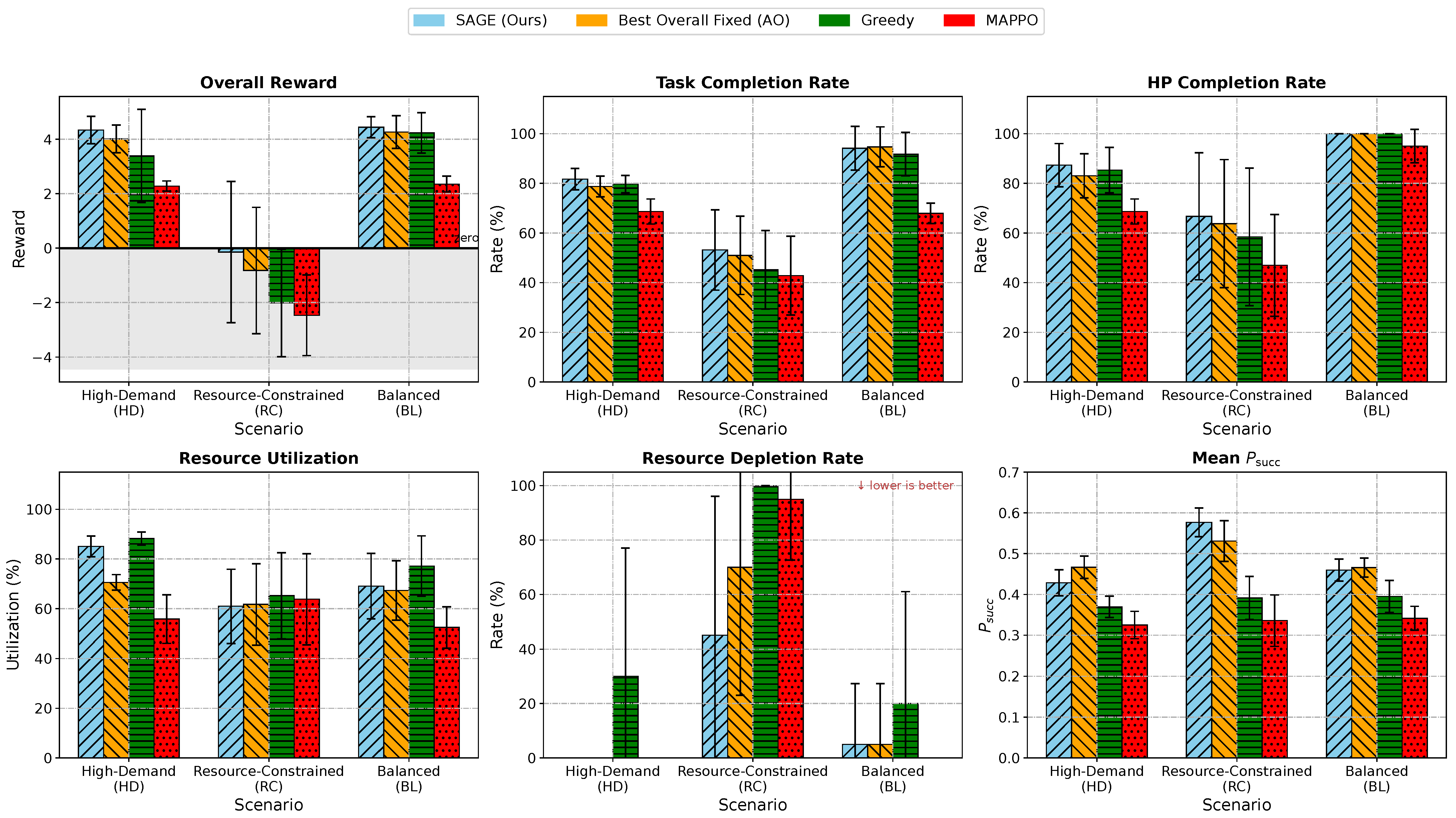
Figure 4 visualizes the per-scenario breakdown across six metrics. The “Best Overall Fixed” bar corresponds to AO, the fixed strategy with the highest average reward across all 60 episodes; note that the per-scenario best fixed strategy differs (MaxO in HD and BL and EO in RC), so AO does not dominate in every individual scenario. In the Overall Reward subplot, all methods yield negative mean rewards under the resource-constrained condition; however, SAGE substantially limits the deficit ($-0.147$) compared to Greedy ($-2.017$), MAPPO ($-2.467$), and the best fixed strategy ($-0.531$) and achieves positive rewards in both the high-demand and balanced scenarios. The Task Completion Rate and HP Completion Rate subplots show that SAGE achieves competitive or leading completion rates across all three scenarios, with the gap over MAPPO particularly pronounced under the high-demand condition. In the Resource Utilization subplot, SAGE maintains balanced utilization without the over-commitment observed in Greedy or the under-utilization seen in MAPPO. The Resource Depletion Rate subplot most clearly illustrates the adaptive advantage: SAGE holds a near-zero depletion rate in the balanced scenario and a substantially lower rate than all baselines in the resource-constrained scenario, where MAPPO reaches approximately 95%. Finally, in the Mean $P_{\mathrm{succ}}$ subplot, SAGE maintains competitive executor–task matching quality across scenarios, confirming that conservative strategy selection under resource pressure does not substantially degrade assignment effectiveness.

5.5. Ablation Study

We conduct three ablation experiments to isolate the contributions of key architectural decisions. Experiment A (

Table 10. Ablation study: GNN architecture components ($2\times 2$ factorial design; mean ± std over 60 evaluation episodes).

Variant	Reward	Compl. Rate	HP Compl.	Res. Util.	Depl. Rate	Mean ${\mathit{P}}_{\mathbf{succ}}$
SAGE (Ours)	2.878 ± 2.637	76.3% ± 20.4%	84.7% ± 20.6%	71.7% ± 15.3%	16.7% ± 37.6%	0.488 ± 0.071
w/o type projection	2.621 ± 2.891	74.1% ± 23.0%	81.9% ± 23.7%	73.9% ± 16.3%	28.3% ± 45.4%	0.486 ± 0.061
$\Delta$	−8.9%	−2.9%	−3.3%	+3.1%	+69.5%	−0.5%
w/o edge features	2.743 ± 2.652	74.8% ± 21.3%	82.8% ± 22.6%	71.6% ± 16.1%	18.3% ± 39.0%	0.479 ± 0.075
$\Delta$	−4.7%	−2.0%	−2.2%	−0.1%	+9.6%	−1.8%
w/o both (HomoGNN)	2.766 ± 2.697	75.6% ± 21.2%	84.3% ± 21.8%	71.8% ± 15.2%	21.7% ± 41.5%	0.475 ± 0.062
$\Delta$	−3.9%	−0.9%	−0.5%	+0.1%	+29.9%	−2.6%
MLP (matched params)	2.646 ± 2.690	75.5% ± 21.6%	83.7% ± 22.3%	68.7% ± 15.1%	23.8% ± 42.9%	0.490 ± 0.064
$\Delta$	−8.1%	−1.0%	−1.2%	−4.2%	+42.5%	+0.5%

) evaluates the GNN encoding module via a factorial design over two binary factors—type-specific node projection and three-dimensional edge features—yielding four GNN variants, together with a parameter-matched MLP baseline that removes graph structure entirely. Experiment B (

Table 11. Ablation study: dynamic vs. fixed per-task executor limit ($M_j$) (mean ± std over 60 evaluation episodes).

Variant	Reward	Compl. Rate	HP Compl.	Res. Util.	Depl. Rate	Mean ${\mathit{P}}_{\mathbf{succ}}$
SAGE (Ours)	2.878 ± 2.637	76.3% ± 20.4%	84.7% ± 20.6%	71.7% ± 15.3%	16.7% ± 37.6%	0.488 ± 0.071
Fixed $M_j=2$	2.753 ± 2.669	76.5% ± 20.7%	84.9% ± 20.6%	72.5% ± 15.6%	18.3% ± 39.0%	0.465 ± 0.066
$\Delta$	−4.3%	+0.3%	+0.2%	+1.1%	+9.6%	−4.9%
Fixed $M_j=3$	2.594 ± 2.573	73.7% ± 19.7%	82.8% ± 20.6%	75.2% ± 15.1%	18.3% ± 39.0%	0.428 ± 0.086
$\Delta$	−9.9%	−3.4%	−2.2%	+4.9%	+9.6%	−12.4%
Fixed $M_j=4$	2.427 ± 2.481	72.2% ± 19.0%	82.0% ± 20.6%	75.5% ± 14.6%	20.0% ± 40.3%	0.411 ± 0.098
$\Delta$	−15.7%	−5.4%	−3.2%	+5.3%	+19.8%	−15.8%

) examines the dynamic per-task executor limit ($M_j$) by substituting it with fixed constants ($M_j\in \{2,3,4\}$), directly testing whether the adaptive limit contributes independently of the meta-controller’s strategy selection. Each variant is evaluated on the same 60 fixed episodes under the shared three-scenario protocol.

Table 10 reveals a clear hierarchy among the GNN variants. The two dominant factors are type-specific projection and graph structure. Removing type-specific projection (w/o type projection) causes the largest single-factor reward drop ($-8.9\%$) and more than doubles the depletion rate ($+69.5\%$), indicating that without separate linear projections for executor and task nodes, the encoder conflates structurally distinct node types and loses the feature contrast needed for conservative resource management. Replacing the entire GNN with a parameter-matched MLP reduces the reward by $8.1\%$ and raises depletion by $42.5\%$, confirming that graph-structured relational encoding—not merely representational capacity—is the primary driver of performance. Removing edge features (w/o edge features) yields a more modest reward penalty ($-4.7\%$) and a moderate depletion increase ($+9.6\%$), suggesting that the three-dimensional edge features contribute positively to assignment quality but are not individually decisive. The homogeneous variant (w/o both) degrades the reward by $3.9\%$ and raises depletion by $29.9\%$; notably, its reward gap is smaller than either single-factor ablation, suggesting partial mutual compensation when both biases are introduced simultaneously.

Table 11 reveals a monotonic degradation pattern as the fixed executor limit increases. A fixed $M_j=2$ incurs a modest reward loss ($-4.3\%$) and a $9.6\%$ depletion increase, as the tight limit passively prevents over-commitment, even without adaptive control. A fixed $M_j=3$ produces a larger reward drop ($-9.9\%$) while sharing the same depletion penalty, indicating that at moderate limits, the system begins to lose assignment flexibility without gaining additional resource safety. A fixed $M_j=4$ is the most damaging configuration: the reward falls by $15.7\%$, the task completion rate drops by $5.4\%$, high-priority completion declines by $3.2\%$, and the mean $P_{\mathrm{succ}}$ plunges by $15.8\%$, suggesting that a permissive fixed limit removes the friction that motivates conservative assignments while simultaneously reducing the effective executor capacity per task. Thus, the dynamic $M_j$ mechanism provides automatic resource pacing that is complementary to rather than redundant for the meta-controller’s discrete strategy selection.

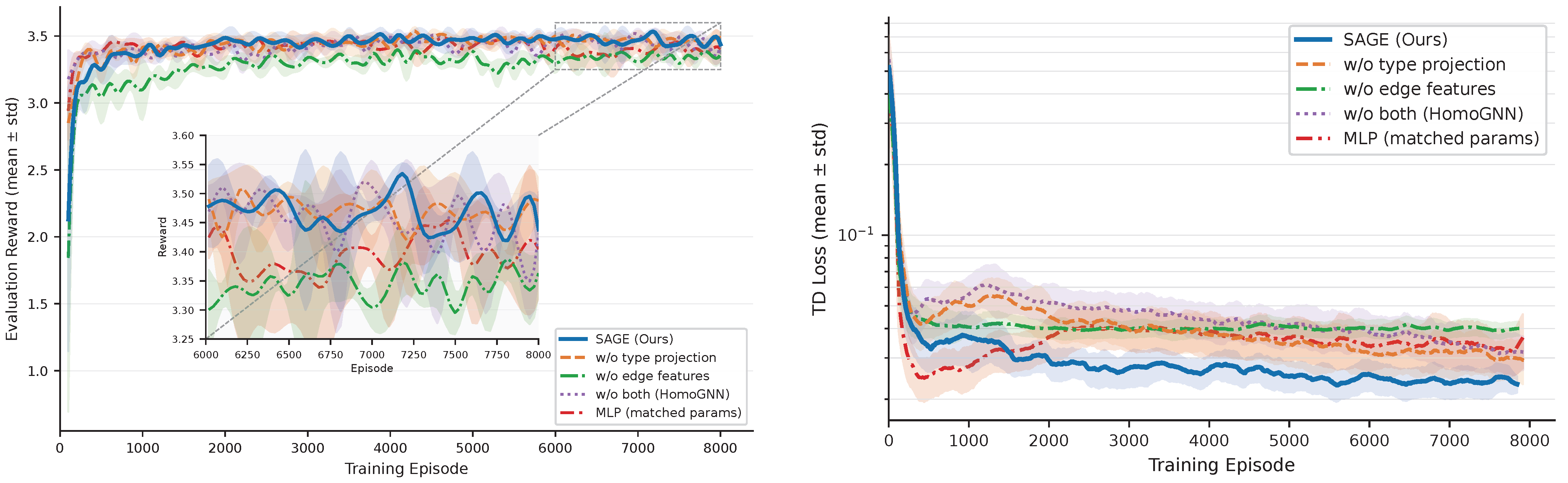
Figure 5 presents the training dynamics of all GNN ablation variants across 8000 episodes. All variants exhibit a rapid initial reward rise within the first 1000 episodes, driven primarily by the MILP solver: once the meta-controller commits to any strategy, the solver immediately produces feasible high-quality assignments, providing a strong reward floor that substantially compresses the exploration phase relative to end-to-end RL approaches. Beyond this early phase, the training curves diverge according to architectural completeness. SAGE sustains steady reward improvement throughout training as the meta-controller progressively refines its scene-to-strategy mapping, whereas ablation variants plateau earlier and at lower reward levels. The TD loss curves mirror this pattern: SAGE achieves the lowest Bellman residual throughout, while ablation variants settle at visibly higher loss levels, indicating weaker Q-function self-consistency. The narrow confidence bands for SAGE across both metrics confirm stable convergence across different random seeds, in contrast to the wider bands of the w/o edge features variant, which reflects increased training variance when relational edge signals are absent.

5.6. Sensitivity Analysis

5.6.1. Depletion Penalty Coefficient ($\delta$)

Table 12. Sensitivity to depletion penalty coefficient ($\delta$) (mean ± std over 60 evaluation episodes; ⋆ denotes the proposed setting).

$\mathit{\delta }$	Reward	Compl. Rate	HP Compl.	Res. Util.	Depl. Rate	Mean ${\mathit{P}}_{\mathbf{succ}}$
0.1	3.150 ± 1.882	75.5% ± 20.8%	84.6% ± 21.4%	72.4% ± 15.7%	25.0% ± 43.7%	0.479 ± 0.068
0.2	2.923 ± 2.305	75.3% ± 21.2%	83.1% ± 22.9%	71.8% ± 15.1%	20.0% ± 40.3%	0.474 ± 0.064
0.3 ⋆	2.878 ± 2.637	76.3% ± 20.4%	84.7% ± 20.6%	71.7% ± 15.3%	16.7% ± 37.6%	0.488 ± 0.071
0.5	2.431 ± 3.550	75.8% ± 21.6%	83.5% ± 22.7%	71.3% ± 14.9%	18.3% ± 39.0%	0.479 ± 0.064

reports the effect of $\delta$ on all six evaluation metrics. At $\delta =0.1$, the agent achieves the highest reward (3.150) but incurs the worst depletion rate (25.0%), indicating that a weak penalty provides insufficient deterrence against resource over-consumption. Increasing $\delta$ to 0.2 reduces depletion to 20.0% at the cost of a moderate reward drop. At $\delta =0.5$, the agent becomes excessively conservative, and the reward falls to 2.431 while task completion and the high-priority hit rate also decline. The selected $\delta =0.3$ achieves the lowest depletion rate (16.7%) while retaining competitive reward (2.878) and the highest completion rates, confirming it as the best-balanced operating point.

5.6.2. Number of Discrete Actions (K)

Table 13. Sensitivity to the number of discrete offloading strategies (K) (mean ± std over 60 evaluation episodes; ⋆ denotes the proposed setting).

K	Reward	Compl. Rate	HP Compl.	Res. Util.	Depl. Rate	Mean ${\mathit{P}}_{\mathbf{succ}}$
3	2.593 ± 2.804	74.9% ± 21.6%	83.9% ± 22.3%	71.5% ± 15.0%	23.3% ± 42.7%	0.472 ± 0.055
4	2.674 ± 2.806	75.6% ± 21.3%	84.4% ± 22.3%	67.5% ± 12.3%	25.0% ± 43.7%	0.487 ± 0.046
5 ⋆	2.878 ± 2.637	76.3% ± 20.4%	84.7% ± 20.6%	71.7% ± 15.3%	16.7% ± 37.6%	0.488 ± 0.071
6	2.840 ± 2.656	74.7% ± 21.7%	82.5% ± 22.4%	71.6% ± 15.1%	18.3% ± 39.0%	0.483 ± 0.070
7	2.765 ± 2.649	75.3% ± 21.6%	83.7% ± 22.0%	71.3% ± 14.9%	20.0% ± 40.3%	0.482 ± 0.066

summarizes the effect of K across all six metrics. $K=5$ achieves the highest reward (2.878) and the lowest depletion rate (16.7%), with the best task completion and high-priority hit rates. At $K=3$, the coarse-grained action space limits the policy’s ability to differentiate between workload scenarios, reducing the reward to 2.593. At $K=4$, resource utilization drops noticeably (67.5%), and depletion rises to 25.0%, suggesting that four strategies cannot adequately cover both aggressive and conservative regimes. For $K\ge 6$, the action space becomes fragmented, making it harder for the agent to associate strategies with specific operational contexts within the fixed 8000-episode training budget, and both reward and completion rates decline monotonically.

5.7. Computational Complexity and Runtime Scalability

Let I denote the number of executor nodes, J represent the number of active tasks, S denote the number of sensing nodes, N = I + J be the graph size used by the HeteroGNN encoder, L be the number of graph message-passing layers, and d represent the hidden dimension. With the dense adjacency representation used in the present implementation, one HeteroGNN forward pass has a time complexity of $O\left(L{N}^{2}d\right)$ and memory complexity of $O(N^2+Nd)$. The MILP stage first enumerates feasible sensing–executor–task candidate chains whose pre-filtered count is upper bounded by $O\left(SIJ\right)$. The resulting mixed-integer optimization problem contains one binary decision variable per feasible candidate chain, together with resource-capacity, task-cardinality, assignment-budget, and feasibility constraints. As with general MILP problems, the worst-case solve complexity is exponential in the number of binary variables; in practice, reachability filtering, success-probability thresholds, dynamic per-task executor limits, and the selected assignment budget substantially reduce the effective candidate set.

To quantify practical runtime scalability,

Table 14. Runtime scalability across increasing problem sizes (mean ± std over 20 cases).

Scale	$(\mathit{S},\mathit{I},\mathit{J})$	Graph Nodes	Candidate Chains	GNN Forward (ms)	MILP Solve (ms)	Total Decision (ms)
Small	(4, 6, 4)	10	94.2 ± 8.0	0.376 ± 0.009	8.01 ± 0.56	8.38 ± 0.56
Original	(8, 12, 8)	20	440.4 ± 35.9	0.401 ± 0.023	24.17 ± 1.69	24.57 ± 1.70
Medium	(12, 18, 12)	30	1272.6 ± 96.5	0.443 ± 0.036	72.83 ± 11.31	73.28 ± 11.31
Large	(16, 24, 16)	40	2284.8 ± 123.0	0.460 ± 0.031	148.57 ± 24.45	149.03 ± 24.46

reports wall-clock decision time across four problem scales. Each scale contains 20 independently generated cases. The MILP timing includes candidate filtering, model construction, SCIP optimization, and solution extraction; HeteroGNN timing is measured by repeated CPU forward passes of the implemented HeteroGNN encoder. All cases are solved to optimality within the 3 s SCIP time limit. At the original evaluation scale, the average total decision time is 24.57 ms. Even at the largest tested scale, with 40 graph nodes and 2284.8 candidate chains, on average, the total decision time remains 149.03 ms, indicating that the proposed two-level learning-optimization pipeline is computationally feasible for the problem sizes considered in this study. The runtime is dominated by the MILP solver, whereas the HeteroGNN forward pass remains below 0.5 ms across all tested scales.

5.8. Scene-Adaptive Strategy Selection Analysis

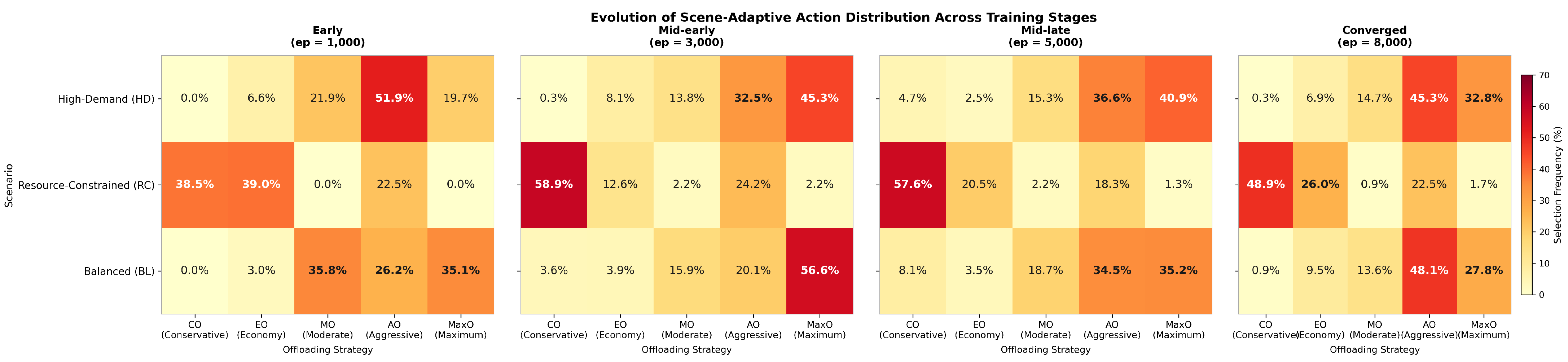
Figure 6 traces the evolution of the learned action distribution across four training stages, providing interpretable evidence of how scene-adaptive behavior emerges over the course of training.

The Resource-Constrained scenario exhibits the earliest and most stable differentiation. As early as episode 1000, the agent already assigns 38.5% to CO and 39.0% to EO, with MaxO entirely absent—indicating that the penalty signal from resource depletion is strong enough to drive conservative preferences within the first training phase. By episode 3000, CO consolidates to 58.9% and remains dominant through convergence (48.9%), confirming that the mapping from resource scarcity to conservative strategy is among the first associations the meta-controller acquires.

In contrast, the High-Demand and Balanced scenarios require more training to differentiate. At episode 1000, the two scenarios show similar distributions, dominated by AO and MO, with the agent not yet reliably distinguishing between them. By episode 3000, the HD distribution shifts toward MaxO (45.3%), while the BL distribution temporarily concentrates on MaxO (56.6%) as well, reflecting an intermediate stage where the agent has learned to be aggressive but has not yet learned to modulate intensity. By convergence, the two scenarios separate clearly: HD stabilizes at AO (45.3%) and MaxO (32.8%), while BL shifts toward AO (48.1%), with a reduced MaxO share (27.8%) and a growing conservative component, reflecting the more moderate resource conditions of the balanced scenario.

To further clarify feature-level interpretability,

Table 15. Feature-level interpretation of workload-dependent strategy selection.

Scenario	Dominant State Cues	Observed Policy Transition	Interpretation
Resource-Constrained	Low executor resource ratio; high depletion risk	CO/EO dominate from the early stage and remain dominant after convergence	Resource scarcity is treated as the primary trigger for conservative assignment budgets.
High-Demand	High task density; high high-priority ratio; sufficient resources	Strategy preference shifts from MO/AO toward AO/MaxO as training progresses	The controller increases assignment intensity when urgent high-value workload justifies larger resource expenditure.
Balanced	Moderate task density; sufficient resources; weaker urgency signal	AO remains dominant, while MaxO is reduced and conservative actions reappear at convergence	The policy avoids unnecessary maximum-budget actions when workload pressure is moderate.

links the dominant situational cues in the seven-dimensional state vector to the observed action-frequency transitions. The analysis shows that the average executor resource ratio is the most decisive cue for conservative policy selection: when the resource ratio is low, the policy rapidly shifts toward CO and EO to suppress depletion. In contrast, high active-task density and a high-priority task ratio increase the preference for AO and MaxO, indicating that the policy uses aggressive strategies mainly when the workload contains enough urgent or valuable tasks to justify higher resource expenditure. Balanced scenarios combine moderate task density with sufficient resources; the policy therefore keeps AO as the dominant action but retains non-negligible conservative selections, preventing the controller from behaving as a uniformly aggressive policy.

Taken together, the four-panel progression confirms that scene discrimination is learned incrementally: resource-constrained recognition emerges early from strong depletion signals, while finer discrimination between high-demand and balanced conditions develops gradually as the meta-controller accumulates sufficient experience to distinguish their subtler differences in task density and resource availability.

6. Conclusions

This paper presented SAGE, a scene-adaptive task-offloading framework for heterogeneous edge networks combining a heterogeneous graph neural network encoder, a dueling double DQN meta-controller, and an MILP solver. The key insight is to decouple task offloading into two levels: a learned meta-controller that perceives the workload scenario through a fused graph-plus-situational-state representation and selects a suitable offloading strategy and a combinatorial solver that executes precise task-chain assignment under the selected configuration.

Experiments on 60 fixed evaluation episodes across three representative workload scenarios demonstrate that SAGE achieves a 15.9% improvement in overall reward over the best fixed-strategy baseline and a 54.1% improvement over a greedy heuristic. Under resource-constrained conditions, SAGE reduces the reward deficit by 72.3% (from $-0.531$ to $-0.147$), driven by the agent’s learned ability to automatically shift toward conservative strategies when executor resources are scarce. Ablation studies confirm the individual contributions of edge-gated GNN encoding, heterogeneous node projection, and the dynamic per-task executor-limit mechanism. Sensitivity analyses identify $\delta =0.3$ and $K=5$ as robust operating points.

The present evaluation is simulation-based, which enables controlled comparison across independently generated and seed-fixed workload scenarios but does not yet replace validation on physical edge-computing testbeds or public operational traces. Future work will therefore validate SAGE under hardware-in-the-loop or real testbed deployments, calibrate the workload generator with operational traces when available, and examine the robustness of the learned strategy-selection policy under sensing noise, communication uncertainty, and device-level execution delays.

Future work will also investigate multi-agent extensions in which decentralized meta-controllers coordinate across multiple edge clusters and the integration of real-time workload prediction to proactively reconfigure assignment strategies before scenario transitions occur.