Optimized Design of Multi-Layer LEO Satellite Constellations for Integrated Communication and Signal-of-Opportunity Doppler Positioning

Abstract

Future low Earth orbit (LEO) communication constellations are evolving into integrated multi-mission infrastructure. Their signals of opportunity (SoP) are therefore becoming attractive for Doppler positioning. However, the conventional coverage- or rate-optimized configurations may not provide favorable Doppler geometry under realistic link-quality constraints. This paper considers this emerging requirement at the constellation-configuration design level and proposes a multi-layer Walker optimization framework for integrated communication and SoP Doppler positioning. A system-level positioning metric is developed to move beyond visibility and dilution-of-precision indicators. A link-quality-constrained multi-epoch Fisher information matrix (FIM) incorporates $C/N_0$-based link measurability and a general carrier-to-noise-density-dependent Doppler-noise formulation. In the reported simulations, $C/N_0$ controls observation admission, while all admitted Doppler observations use a fixed noise standard deviation of 0.5 m/s. An effective position-error bound is then obtained by marginalizing clock-drift and frequency-bias nuisance states. Based on a unified satellite–ground geometry, weighted service coverage, weighted best-link achievable rate, and the proposed positioning metric are jointly optimized using a constrained mixed-integer multi-objective artificial hummingbird algorithm (CMI-MOAHA). The FIM-based metric is consistent with the positioning root mean square error (RMSE) from a separately implemented nonlinear Doppler solver under matched observation and noise assumptions. With the total number of satellites fixed at 2000, the Pareto archive reveals clear trade-offs among coverage, best-link achievable rate, and positioning. When the positioning objective is included, the best obtained positioning metric decreases across all tested constellation sizes, with a maximum reduction of 77.1%. These results show that constellation-level joint optimization is warranted when LEO communication satellites also serve as SoP for Doppler positioning.

1. Introduction

Low Earth orbit (LEO) satellite constellations are becoming key infrastructure for future space–air–ground integrated networks because they can provide low-latency, wide-area, and flexible non-terrestrial services [1,2]. Their system-level performance is mainly determined by constellation configuration. Comparative studies of broadband LEO systems have shown that orbital altitude, inclination, number of orbital planes, and satellite distribution lead to different trade-offs among coverage, capacity, latency, and deployment scale [3]. Recent surveys further indicate that LEO constellation design is moving from single-purpose systems toward integrated communication, positioning, sensing, and network-level services [4]. Walker constellations provide a compact representation of this design space [5]; for example, Wei et al. [6] used Walker parameters to design an efficient LEO global navigation constellation satisfying multiple-coverage and position dilution of precision (PDOP) constraints.

Communication-oriented constellation design has progressed from geometric coverage to service-aware optimization. Jiang et al. [7] optimized a regional LEO constellation according to user requirements and satellite cost. Deng et al. [8] studied ultra-dense LEO deployment for global terrestrial-satellite backhaul, and Wang et al. [9] showed that multi-layer constellations can reduce the number of satellites required for seamless coverage under traffic-sensitive backhaul requirements. More recent work has incorporated user-distribution matching [10], genetic-algorithm-based mega-constellation coverage optimization [11], diversified quality-of-service (QoS) and capacity constraints [12], and regional traffic demand and network invulnerability [13]. These studies clarify how constellation geometry affects communication services but do not include positioning performance as a design objective.

Studies of integrated and multi-mission constellations are more closely related to the present work. Yang et al. [14] and Huang et al. [15] investigated the design of LEO communication–navigation constellations, while Qin et al. [16] considered a cross-domain fusion constellation for communication, navigation, and remote sensing. Guan et al. [17] optimized Walker constellations for LEO-based Global Navigation Satellite System (GNSS) augmentation, and Xu et al. [18] studied multi-layer LEO constellation optimization for GLONASS augmentation. Wang et al. [19] studied composite multi-layer LEO constellations with communication and navigation functions, and Pan et al. [20] proposed a unified framework for hybrid LEO constellations. Several of these studies exploit multi-layer orbital diversity, but they generally characterize positioning using visibility, geometric dilution of precision (GDOP), PDOP, or resource-coverage indicators rather than Doppler positioning accuracy under link-quality constraints.

LEO signals of opportunity (SoP) further motivate integrated constellation design. Morales-Ferre et al. [21] compared existing LEO constellations using code- and Doppler-based GDOP. Psiaki [22] demonstrated the potential of carrier-Doppler navigation using large LEO constellations, and Baron et al. [23] derived practical Doppler navigation Jacobians and dilution metrics. Allahvirdi-Zadeh et al. [24] evaluated multi-constellation broadband LEO Doppler positioning under realistic observation restrictions. A recent survey summarizes LEO SoP positioning [25], while related work has examined clock-error compensation and ill-conditioned Doppler positioning equations [26,27]. These works provide an observation-level foundation for LEO Doppler positioning but generally evaluate existing constellations rather than optimizing constellation configurations jointly for positioning and communication performance.

Satellite links may also be affected by external interference. Zhang et al. [28] analyzed spatially random interference in satellite–aerial downlinks, while Liu et al. [29] investigated time-domain anti-jamming methods for satellite navigation receivers. More recently, jamming-signal recognition and classification have been studied to support the selection of anti-jamming strategies [30]. These studies address interference at the link and receiver levels, whereas the implications of interference for integrated communication and SoP constellation design remain less explored.

The remaining gap therefore lies at the constellation-design level. GDOP/PDOP metrics characterize observation geometry, whereas visible-satellite counts characterize observation availability; neither directly captures link-dependent measurability or noise. In SoP Doppler positioning, received link quality can affect both whether an observation is usable and the noise it contributes. A constellation optimized only for coverage or rate may therefore lack sufficient multi-epoch Doppler observability. This motivates a constellation-level optimization model that evaluates communication links and Doppler positioning using the same satellite–ground geometry. The model represents Doppler positioning performance with a link-quality-constrained, multi-epoch Fisher information matrix (FIM)-based objective.

Table 1. Comparison of representative LEO constellation configuration optimization studies.

Study	Type and Architecture	Positioning Metric	Communication Metric	Link-Quality Model	Optimization Variables
Qin et al. [16] (2023)	Communication + navigation + remote sensing; cross-domain fusion	GDOP	Resource coverage	Resource-level service model	$h,i,N$, payload deployment
Sun et al. [10] (2025)	Communication; Walker-Delta constellation	Not considered	User-distribution matching and access performance	Access-performance model	$h,i,T/P/F$
Zhao et al. [12] (2025)	Communication; dual-layer LEO constellation	Not considered	QoS, capacity, coverage, and cost	QoS/capacity constraints	$h_l,i_l,P_l,S_l$, $l=1,2$
Wang et al. [19] (2025)	Communication + navigation; multi-layer composite LEO	PDOP	Not jointly optimized as an objective	Not Doppler-FIM-based	$h,i,N/P/F,l$
Pan et al. [20] (2026)	Communication + navigation + remote sensing; hybrid LEO	Visibility uniformity and PNTRC capability	Coverage and service capability	Not Doppler-FIM-based	$h,i,P,S,C_{\mathsf{\Omega }},C_F$
This work (2026)	Communication + SoP positioning; multi-layer Walker	Link-quality-constrained multi-epoch Doppler FIM with $a_{\mathrm{pos}}\left(Y\right)$	Weighted best-link achievable rate	Link-budget model + Doppler-noise weighting	$h_l,i_l,P_l,S_l$, $l=1,\dots ,L$

compares representative studies across the relevant design dimensions.

To address this gap, this paper proposes a multi-layer LEO constellation optimization framework for integrated communication and SoP Doppler positioning. The constellation is represented as $Y=\left(Y^{\left(1\right)},Y^{\left(2\right)},\dots ,Y^{\left(L\right)}\right)$, where the l-th layer is parameterized by $Y^{\left(l\right)}=\left(h_l,i_l,P_l,S_l\right)$, $l=1,\dots ,L$. With the total number of satellites fixed at $N_{\mathrm{total}}$, the framework optimizes the altitude, inclination, number of orbital planes, and satellites per plane for each independently configured layer. This structure allows coverage continuity, link quality, and Doppler-geometry diversity to be balanced within a fixed satellite budget. The objectives are the weighted service coverage $f_{\mathrm{cov}}\left(Y\right)$, the weighted best-link achievable-rate metric $f_{\mathrm{com}}\left(Y\right)$, and the FIM-based positioning metric $g_{\mathrm{pos}}\left(Y\right)$, with the positioning availability $a_{\mathrm{pos}}\left(Y\right)$ imposed as a reliability constraint.

The main contributions of this paper are summarized as follows.

• A multi-layer Walker constellation model and a weighted global service model are established for integrated communication and SoP Doppler positioning. Multiple independently configured orbital layers are optimized with the total number of satellites fixed at $N_{\mathrm{total}}$, and $f_{\mathrm{cov}}\left(Y\right)$ and $f_{\mathrm{com}}\left(Y\right)$ are evaluated using ground-cell weights and satellite–ground link conditions.
• A link-quality-constrained multi-epoch FIM-based Doppler positioning metric is developed for constellation-level optimization. Unlike visible-satellite counts and GDOP- or PDOP-based indicators, the metric formulates Doppler observations in the pseudo-range-rate domain, incorporates link measurability, provides a general formulation for link-quality-dependent measurement noise, and obtains effective position information after marginalizing the receiver-common bias, drift, and time-tag states.
• The constellation design problem is formulated as a constrained mixed-integer multi-objective optimization problem with objectives $-f_{\mathrm{cov}}\left(Y\right)$, $-f_{\mathrm{com}}\left(Y\right)$, and $g_{\mathrm{pos}}\left(Y\right)$, subject to the fixed total number of satellites and the positioning-availability constraint $a_{\mathrm{pos}}\left(Y\right)\ge a_{min}$. A CMI-MOAHA method is developed for the mixed-integer Pareto search. Numerical experiments examine the proposed metric, analyze the trade-offs among coverage, best-link achievable rate, and positioning, and compare the optimized dual-layer constellation with a single-layer Walker architecture and reference constellation designs under the adopted evaluation model.

2. System Modeling

2.1. Multi-Layer Walker Constellation Configuration Modeling

A multi-layer Walker constellation is adopted for optimization. Compared with optimizing the orbital parameters of individual satellites, the Walker structure characterizes the constellation using a compact set of parameters, thereby reducing the dimensionality of the system-level design problem. For L independently designed orbital layers, the constellation configuration is denoted by $Y=\left(Y^{\left(1\right)},Y^{\left(2\right)},\dots ,Y^{\left(L\right)}\right)$, where $Y^{\left(l\right)}=\left(h_l,i_l,P_l,S_l\right)$, $l=1,\dots ,L$, represents the configuration of the l-th layer. Here, $h_l$ and $i_l$ denote the orbital altitude and inclination, respectively. $P_l$ is the number of orbital planes, and $S_l$ is the number of satellites per plane. Thus, the number of satellites in the l-th layer is $N_{\mathrm{sat}}^{\left(l\right)}=P_l{S}_l$, and the total number of satellites is $N_{\mathrm{sat}}={\sum }_{l=1}^L{P}_l{S}_l$.

All satellites within a layer are assumed to follow circular orbits at the same altitude and inclination, while the layers are configured independently. The semi-major axis of the l-th layer is $a_l=R_{\mathrm{E}}+h_l$, where $R_{\mathrm{E}}$ is the mean Earth radius. The Walker phase factor is fixed at $F_0$ and is not optimized. The satellite states are propagated from these orbital elements and transformed into the Earth-centered Earth-fixed frame with Earth rotation accounted for. The position and velocity of satellite k at time t are denoted by ${\mathbf{r}}_k(t;Y)$ and ${\mathbf{v}}_k(t;Y)$, respectively, where $k=1,2,\dots ,N_{\mathrm{sat}}$. Thus, Y determines the spatiotemporal distribution of the constellation and serves as the decision variable in the subsequent system-level optimization.

2.2. Ground Modeling

To evaluate constellation configuration Y at the system level, the Earth’s surface is discretized into a finite number of ground service cells. An equal-latitude–longitude grid samples high-latitude regions more densely and may introduce latitude-dependent statistical bias. An approximate equal-area partitioning method is therefore adopted [10]. The global service region is divided into Q ground cells of approximately equal area, denoted by $\mathcal{K}=\{K_q\mid q=1,2,\dots ,Q\}$. Each cell $K_q$ is represented by its geometric center, whose longitude and latitude are denoted by $({\lambda }_q,{\phi }_q)$.

To represent spatially nonuniform service demand, each ground cell is assigned a weight ${\omega }_q$. Following user-demand-oriented LEO constellation design methods [7], the weight combines a global baseline term, a population term, a terrestrial infrastructure term, and a remote-region compensation term. The population and infrastructure terms are derived from the Gridded Population of the World Version 4 (GPWv4) population-density dataset distributed through the National Aeronautics and Space Administration (NASA) Socioeconomic Data and Applications Center (SEDAC) and the OpenCellID cell-tower dataset, respectively [31,32].

Let $po{p}_q$ and $bas{e}_q$ denote the normalized population density and normalized base-station density of $K_q$, respectively. The compensation term is defined as $promot{e}_q=1-max\left(po{p}_q,bas{e}_q\right)$. The service weight of $K_q$ is then given by

$${\omega }_q={\alpha }_0+{\alpha }_{1}po{p}_q+{\alpha }_{2}bas{e}_q+{\alpha }_{3}promot{e}_q,$$

(1)

where ${\alpha }_0$, ${\alpha }_1$, ${\alpha }_2$, and ${\alpha }_3$ are adjustable weighting coefficients satisfying ${\alpha }_0+{\alpha }_1+{\alpha }_2+{\alpha }_3=1$. Here, ${\alpha }_0$ sets the baseline weight, ${\alpha }_1$ and ${\alpha }_2$ control the population and infrastructure terms, and ${\alpha }_3$ controls the remote-region compensation. The weights are then normalized to satisfy ${\sum }_{q=1}^Q{\omega }_q=1$.

This ground model provides representative cell positions and spatial weights for the coverage, best-link achievable-rate, and SoP positioning metrics.

2.3. Single-Satellite Coverage and Service Coverage Metric

Coverage performance characterizes whether a constellation can provide continuous and effective service over the target ground region. A satellite overpass alone does not guarantee service availability because the satellite–ground link must also satisfy the minimum elevation angle, link-quality threshold, and minimum number of serviceable satellites. The single-satellite geometric coverage model is therefore combined with link-quality constraints to define cell-level service coverage and the weighted global objective.

The geometric coverage of a single satellite is determined first. Following the basic LEO constellation coverage model in [7], let $R_{\mathrm{E}}$ denote the Earth radius, $h_k$ denote the orbital altitude of satellite k, and ${\theta }_{min}$ denote the minimum service elevation angle. The auxiliary angle associated with the satellite–ground geometry is given by

$${\psi }_k=arcsin\left({\displaystyle \frac{R_{\mathrm{E}}}{R_{\mathrm{E}}+h_k}}cos{\theta }_{min}\right).$$

(2)

The corresponding single-satellite coverage area on the Earth surface is

$$S_k=2\pi R_{\mathrm{E}}^2\left[1-sin\left({\theta }_{min}+{\psi }_k\right)\right].$$

(3)

For a fixed ${\theta }_{min}$, a higher orbit usually enlarges $S_k$ but also increases the satellite–ground propagation distance. Geometric coverage is therefore necessary but insufficient for service availability; link quality must also be considered.

For ground cell $K_q$ at time t, the geometric visibility set is

$${\mathcal{V}}_q(t;Y)=\left\{k:{\theta }_{qk}(t;Y)\ge {\theta }_{min}\right\}.$$

(4)

The received power is computed from a compact link-budget model,

$$P_{qk}^{\mathrm{rx}}(t;Y)={\displaystyle \frac{P_k^{\mathrm{tx}}{G}_k^{\mathrm{tx}}\left({\alpha }_{qk}(t;Y)\right)G_q^{\mathrm{rx}}\left({\theta }_{qk}(t;Y)\right)}{L_{qk}^{\mathrm{tot}}\left(d_{qk}(t;Y),{\theta }_{qk}(t;Y)\right)}},d_{qk}(t;Y)=∥{\mathbf{r}}_k(t;Y)-{\mathbf{u}}_q∥.$$

(5)

Here, $P_k^{\mathrm{tx}}{G}_k^{\mathrm{tx}}\left({\alpha }_{qk}\right)$ is the direction-dependent satellite equivalent isotropically radiated power (EIRP), $G_q^{\mathrm{rx}}\left({\theta }_{qk}\right)$ is the receive antenna gain, and $L_{qk}^{\mathrm{tot}}$ includes free-space path loss, atmospheric and rain attenuation, polarization loss, and other distance- and elevation-dependent losses. The instantaneous received signal-to-noise ratio (SNR) and carrier-to-noise-density ratio ($C/N_0$) are then

$${\mathsf{\Gamma }}_{qk}(t;Y)={\displaystyle \frac{P_{qk}^{\mathrm{rx}}(t;Y)}{N_0{B}_q}},{\left({\displaystyle \frac{C}{N_0}}\right)}_{qk}(t;Y)={\displaystyle \frac{P_{qk}^{\mathrm{rx}}(t;Y)}{N_0}}={\mathsf{\Gamma }}_{qk}(t;Y)B_q.$$

(6)

The positioning-observable and communication-serviceable satellite sets are defined as

$${\mathcal{M}}_q(t;Y)=\left\{k\in {\mathcal{V}}_q(t;Y):{\left(C/N_0\right)}_{qk}(t;Y)\ge {\left(C/N_0\right)}_{\mathrm{meas}}\right\},$$

(7)

$${\mathcal{S}}_q(t;Y)=\left\{k\in {\mathcal{V}}_q(t;Y):{\mathsf{\Gamma }}_{qk}(t;Y)\ge {\mathsf{\Gamma }}_{\mathrm{srv}}\right\}.$$

(8)

Here, ${(C/N_0)}_{\mathrm{meas}}$ is the SoP Doppler measurement threshold, and ${\mathsf{\Gamma }}_{\mathrm{srv}}$ is the communication service threshold.

The two sets are evaluated sequentially using different receive-gain directions. During service-link screening, $G_q^{\mathrm{rx}}$ is evaluated at boresight, and the satellite with the highest SNR in ${\mathcal{S}}_q(t;Y)$ is selected as the serving satellite. Its direction defines the receiver boresight for positioning-link screening. The receive gain of each visible positioning candidate is then evaluated at its angular separation from this direction. If ${\mathcal{S}}_q(t;Y)$ is empty, no receiver boresight is defined and no positioning observation is admitted. Thus, ${\mathcal{M}}_q(t;Y)$ and ${\mathcal{S}}_q(t;Y)$ remain distinct, while ${\mathsf{\Gamma }}_{\mathrm{srv}}$ affects positioning only indirectly through service availability and receiver pointing.

The link-budget model assumes nominal noise-limited operation and excludes external intentional interference. Such interference can reduce effective link quality and degrade Doppler estimation, while jamming-signal detection and classification can support the selection of anti-jamming strategies [30]. The reported results therefore apply to nominal non-jammed conditions.

The coverage metric is based on ${\mathcal{S}}_q(t;Y)$. Satellite k provides effective service coverage for $K_q$ at time t if $k\in {\mathcal{S}}_q(t;Y)$. Let $K_{\mathrm{cov}}$ denote the minimum number of serviceable satellites required for coverage. The coverage status of $K_q$ is

$$C_q^{\mathrm{cov}}(t;Y)=\left\{\begin{array}{cc}1,\hfill & \left|{\mathcal{S}}_q(t;Y)\right|\ge K_{\mathrm{cov}},\hfill \\ 0,\hfill & \left|{\mathcal{S}}_q(t;Y)\right|<K_{\mathrm{cov}}.\hfill \end{array}\right.$$

(9)

The case $K_{\mathrm{cov}}=1$ corresponds to basic service coverage, while $K_{\mathrm{cov}}>1$ represents a multiple-coverage requirement.

For a simulation set $\mathcal{T}$ with T time samples, the time-averaged coverage ratio of $K_q$ is

$$f_{\mathrm{cov},q}\left(Y\right)={\displaystyle \frac{1}{T}}{\displaystyle \sum _{t=1}^T}{C}_q^{\mathrm{cov}}(t;Y).$$

(10)

Aggregating all cells with the spatial weights ${\omega }_q$ gives the global coverage objective

$$f_{\mathrm{cov}}\left(Y\right)={\displaystyle \sum _{q=1}^Q}{\omega }_q{f}_{\mathrm{cov},q}\left(Y\right).$$

(11)

Thus, the coverage optimization objective is to maximize $f_{\mathrm{cov}}\left(Y\right)$.

2.4. Weighted Best-Link Achievable-Rate Metric

The weighted best-link achievable-rate metric is evaluated over the communication-serviceable set ${\mathcal{S}}_q(t;Y)$ defined in Section 2.3. It characterizes how constellation geometry affects the strongest serviceable satellite–ground link through satellite visibility, link distance, antenna gain, and received signal-to-noise ratio. For each ground cell and time sample, the serviceable satellite with the largest Shannon achievable rate is selected. The resulting values are averaged over time and aggregated using the spatial weights [33].

The metric isolates the effect of constellation geometry and does not represent network-level resource allocation. Each ground cell is evaluated independently under a common reference bandwidth and transmit-power setting. No cross-cell coupling is imposed through satellite beam limits, power allocation, bandwidth sharing, user association, or co-channel interference, and feeder-link capacity is not constrained. Multiple cells may therefore select the same satellite without sharing its resources. Under these assumptions, $f_{\mathrm{com}}\left(Y\right)$ describes the achievable-rate potential of the best satellite–ground links supported by the constellation geometry rather than aggregate network throughput.

For ground cell $K_q$ and satellite $k\in {\mathcal{S}}_q(t;Y)$, the instantaneous achievable rate at time t is defined as

$$R_{qk}(t;Y)=B_q{log}_2\left(1+{\mathsf{\Gamma }}_{qk}(t;Y)\right),$$

(12)

where $B_q$ is the reference bandwidth of $K_q$, and ${\mathsf{\Gamma }}_{qk}(t;Y)$ is the instantaneous received signal-to-noise ratio.

At each time instant, $K_q$ selects the satellite with the largest achievable rate from ${\mathcal{S}}_q(t;Y)$. If ${\mathcal{S}}_q(t;Y)\ne \varnothing$, the serving satellite index is $k_q^{★}(t;Y)=arg{max}_{k\in {\mathcal{S}}_q(t;Y)}{R}_{qk}(t;Y)$. The instantaneous best-link achievable rate of $K_q$ is then

$$R_q(t;Y)=\left\{\begin{array}{cc}{R}_{q{k}_q^{★}(t;Y)}(t;Y),\hfill & {\mathcal{S}}_q(t;Y)\ne \varnothing ,\hfill \\ 0,\hfill & {\mathcal{S}}_q(t;Y)=\varnothing .\hfill \end{array}\right.$$

(13)

Thus, the rate is zero when no satellite satisfies the communication service threshold.

For a simulation set $\mathcal{T}$ with T time samples, the time-averaged best-link achievable rate of $K_q$ is

$$f_{\mathrm{com},q}\left(Y\right)={\displaystyle \frac{1}{T}}{\displaystyle \sum _{t=1}^T}{R}_q(t;Y).$$

(14)

Aggregating all cells with the spatial weights ${\omega }_q$ gives

$$f_{\mathrm{com}}\left(Y\right)={\displaystyle \sum _{q=1}^Q}{\omega }_q{f}_{\mathrm{com},q}\left(Y\right).$$

(15)

The metric $f_{\mathrm{com}}\left(Y\right)$ represents the weighted time-averaged best-link achievable rate over the ground service region. Higher values indicate better best-link performance under the stated assumptions; the objective is therefore to maximize $f_{\mathrm{com}}\left(Y\right)$.

2.5. SoP Positioning Performance Metric

LEO communication constellations can support both broadband services and Doppler positioning because of their high orbital velocities and wide-area visibility. Doppler positioning exploits the line-of-sight relative motion between satellites and receivers; the resulting carrier-frequency shift constrains the receiver position. Unlike dedicated navigation constellations, communication satellites are not primarily designed for positioning. Their positioning capability depends on satellite–ground geometry, link measurability, Doppler measurement noise, and non-geometric error sources. Consequently, visible-satellite counts and conventional geometric dilution indicators do not fully characterize SoP positioning performance under communication-link constraints. This subsection develops a multi-epoch FIM-based position-error lower-bound metric for constellation configuration Y by combining pseudo-range-rate observations, link-quality-dependent noise, nuisance-state marginalization, and positioning availability.

2.5.1. Pseudo-Range-Rate Observation Model

The Doppler measurement is first expressed in the pseudo-range-rate domain, removing the direct dependence of the observation magnitude on carrier frequency when different satellites or signals use different wavelengths. Following common LEO Doppler navigation and SoP positioning models [22,23,24], let ${\lambda }_k$ denote the wavelength of satellite k, and let $f_{D,qk,m}$ denote the Doppler shift observed by ground cell $K_q$ at the m-th sampling epoch. The pseudo-range-rate observation is defined as $z_{qk,m}=-{\lambda }_k{f}_{D,qk,m}$, where the negative sign follows the range-rate convention and $z_{qk,m}$ is expressed in $\mathrm{m}/\mathrm{s}$.

For a static ground cell located at ${\mathbf{u}}_q$, the theoretical pseudo-range rate induced by satellite k at epoch $t_m$ is

$${\widehat{\rho }}_{qk,m}({\mathbf{u}}_q;Y)={\displaystyle \frac{{\left({\mathbf{r}}_k(t_m;Y)-{\mathbf{u}}_q\right)}^T{\mathbf{v}}_k(t_m;Y)}{∥{\mathbf{r}}_k(t_m;Y)-{\mathbf{u}}_q∥}}.$$

(16)

This term is the projection of the satellite velocity onto the satellite–ground line of sight. The constellation configuration Y therefore affects Doppler positioning through the satellite positions and velocities.

Practical SoP Doppler observations contain receiver frequency-reference and time-tag errors, together with satellite-dependent transmitter, ephemeris, and propagation errors. Established carrier-Doppler formulations distinguish receiver- and satellite-side errors by jointly estimating receiver clock offset and clock-rate states with the receiver state while representing satellite ephemerides and transmitter clock-frequency terms separately for each link [22,23,24]. Following this convention, the constellation-level metric models the receiver-side residuals with ${\mathsf{\eta }}_q={[{\beta }_q,{\dot{\beta }}_q,\delta {\tau }_q]}^T$. Here, ${\beta }_q$ and ${\dot{\beta }}_q$ represent a receiver-common pseudo-range-rate bias and its drift, and $\delta {\tau }_q$ is the receiver time-tag mismatch. This common state represents errors shared at the receiver rather than a common oscillator error across independent satellite transmitters.

Within one observation window, the receiver-common bias is approximated as $b_q\left(t_m\right)\approx {\beta }_q+{\dot{\beta }}_q(t_m-\tau )$, where $\tau$ is the starting epoch. This constant-plus-linear form provides a first-order model of a smoothly varying receiver frequency reference over a short interval [26]. The equivalent time-offset state is introduced through

$${\widehat{\rho }}_{qk}(t_m+\delta {\tau }_q;{\mathbf{u}}_q,Y)\approx {\widehat{\rho }}_{qk}(t_m;{\mathbf{u}}_q,Y)+g_{qk,m}\delta {\tau }_q,$$

(17)

where $g_{qk,m}={\left.\partial {\widehat{\rho }}_{qk}(t;{\mathbf{u}}_q,Y)/\partial t\right|}_{t=t_m}$ is the local range-acceleration sensitivity of the Doppler observation. This low-dimensional first-order model [26] captures residual effects common to the receiver observations but excludes independent satellite oscillator offsets, higher-order clock variations, ephemeris errors, and abrupt propagation anomalies. These effects require corresponding satellite-specific or time-varying terms [22,24].

The single-link pseudo-range-rate observation model is then

$$z_{qk,m}={\widehat{\rho }}_{qk,m}({\mathbf{u}}_q;Y)+{\beta }_q+{\dot{\beta }}_q(t_m-\tau )+g_{qk,m}\delta {\tau }_q+{\nu }_{qk,m},$$

(18)

where ${\nu }_{qk,m}$ denotes the Doppler pseudo-range-rate measurement noise.

2.5.2. Multi-Epoch Observation Window and General Link-Quality-Dependent Noise Formulation

A single Doppler observation provides only one line-of-sight range-rate constraint. Rapid LEO motion changes the satellite–ground geometry over short intervals, allowing multi-epoch observations to provide stronger position information. For an observation window starting from $\tau$, the sampling epoch set is ${\mathcal{T}}_{\tau }=\{t_m=\tau +m\mathsf{\Delta }t,m=0,1,\dots ,M-1\}$, where $\mathsf{\Delta }t$ is the sampling interval and M is the number of samples. The window length is $T_{\mathrm{obs}}=(M-1)\mathsf{\Delta }t$.

Only satellites in the positioning-observable set ${\mathcal{M}}_q(t_m;Y)$ are used. The available observation set in the window is

$${\mathcal{O}}_q(\tau ;Y)=\left\{(k,m):t_m\in {\mathcal{T}}_{\tau },k\in {\mathcal{M}}_q(t_m;Y)\right\}.$$

(19)

Thus, observation availability depends jointly on the constellation configuration, visibility, and link measurability.

The measurement variance depends on link quality. The carrier-to-noise-density ratio is

$${\left({\displaystyle \frac{C}{N_0}}\right)}_{qk,m}={\displaystyle \frac{P_{qk}^{\mathrm{rx}}(t_m;Y)}{N_0}}={\mathsf{\Gamma }}_{qk}(t_m;Y)B_q,$$

(20)

where $P_{qk}^{\mathrm{rx}}(t_m;Y)$ is the received power, $N_0$ is the noise power spectral density, and $B_q$ is the reference bandwidth.

Based on the Cramer–Rao lower bound for frequency estimation or the thermal-noise approximation of carrier tracking, the Doppler frequency-estimation error variance is modeled as [34,35,36]

$${\sigma }_{f,qk,m}^2={\displaystyle \frac{{\kappa }_f}{{\left(C/N_0\right)}_{qk,m}{T}_{\mathrm{int}}^3}}+{\sigma }_{f,\mathrm{floor}}^2,$$

(21)

where ${\kappa }_f$ depends on the waveform and frequency estimator, $T_{\mathrm{int}}$ is the equivalent coherent integration time, and ${\sigma }_{f,\mathrm{floor}}^2$ is the frequency-estimation error floor determined by the tracking architecture and receiver hardware. The corresponding pseudo-range-rate noise variance is

$${\sigma }_{qk,m}^2={\lambda }_k^2{\sigma }_{f,qk,m}^2+{\sigma }_{\mathrm{mp}}^2\left({\theta }_{qk,m}\right),$$

(22)

where ${\sigma }_{\mathrm{mp}}^2\left({\theta }_{qk,m}\right)$ denotes the elevation-dependent residual multipath and propagation term. This term can be set to zero when environment-dependent errors are not modeled. The measurement noise is therefore ${\nu }_{qk,m}\sim \mathcal{N}\left(0,{\sigma }_{qk,m}^2\right)$. Link quality affects positioning performance through both observation availability and the Fisher-information weight $1/{\sigma }_{qk,m}^2$. Equations (21) and (22) provide a general signal-specific noise formulation whose parameters are selected for the signal and receiver under consideration.

2.5.3. Fisher Information Matrix

The position-error lower bound is derived from the Fisher information matrix [35,36]. After linearizing the observation model around $({\mathbf{u}}_q,{\mathsf{\eta }}_q)$, let ${\rho }_{qk,m}=∥{\mathbf{r}}_k(t_m;Y)-{\mathbf{u}}_q∥$ and ${\mathbf{e}}_{qk,m}=({\mathbf{r}}_k(t_m;Y)-{\mathbf{u}}_q)/{\rho }_{qk,m}$ denote the satellite–ground distance and the line-of-sight unit vector, respectively. The Jacobian with respect to the position parameter is

$${\mathbf{h}}_{u,qk,m}={\displaystyle \frac{\partial {\widehat{\rho }}_{qk,m}({\mathbf{u}}_q;Y)}{\partial {\mathbf{u}}_q}}=-{\displaystyle \frac{{\mathbf{v}}_k^T(t_m;Y)\left(\mathbf{I}-{\mathbf{e}}_{qk,m}{\mathbf{e}}_{qk,m}^T\right)}{{\rho }_{qk,m}}}.$$

(23)

This term shows that Doppler positioning depends on both line-of-sight geometry and satellite velocity.

The Jacobian with respect to the nuisance state is ${\mathbf{h}}_{\eta ,qk,m}=[1,t_m-\tau ,g_{qk,m}]$, and the total Jacobian of one observation is ${\mathbf{H}}_{qk,m}=\left[{\mathbf{h}}_{u,qk,m}{\mathbf{h}}_{\eta ,qk,m}\right]$. Local identifiability of the nuisance parameters requires the stacked nuisance-state Jacobian to have full column rank. Multiple epochs provide the temporal variation needed to distinguish ${\beta }_q$ from ${\dot{\beta }}_q$, while variation in $g_{qk,m}$ across satellites and epochs distinguishes $\delta {\tau }_q$ from these two states. Joint position–nuisance identifiability further requires the stacked ${\mathbf{H}}_{qk,m}$ to have full column rank and acceptable conditioning, consistent with multi-epoch Doppler observability analyses [22,23].

The FIM is conditioned on the nominal ground-cell position and constellation geometry. For each candidate Y, the distance, elevation angle, $C/N_0$, and measurement variance are first evaluated at ${\mathbf{u}}_q$. During the subsequent local linearization, these variances are treated as known fixed weights, as in conventional weighted Doppler-positioning formulations [22,23,24]. The resulting conditional, or frozen-covariance, observation FIM within window $\tau$ is

$${\mathbf{J}}_q^{\mathrm{obs}}(\tau ;Y)=\sum _{(k,m)\in {\mathcal{O}}_q(\tau ;Y)}{\displaystyle \frac{1}{{\sigma }_{qk,m}^2}}{\mathbf{H}}_{qk,m}^T{\mathbf{H}}_{qk,m}.$$

(24)

Equation (24) therefore contains the Jacobian contribution from the conditional measurement mean but no derivative of the measurement covariance. If the position dependence of the covariance were treated as information, the full Gaussian FIM would include an additional covariance-derivative trace term. This extension is outside the conditional model adopted here; the derivative term vanishes for constant measurement covariance.

The nuisance states may also be constrained by clock-calibration or receiver-characterization information available before the current window. This information is represented by the prior covariance matrix

$${\mathbf{Q}}_{\eta ,q}=\mathrm{diag}\left({\sigma }_{\beta ,q}^2,{\sigma }_{\dot{\beta },q}^2,{\sigma }_{\tau ,q}^2\right),$$

(25)

with the corresponding prior information matrix

$${\mathbf{J}}_q^{\mathrm{prior}}=\left[\begin{array}{cc}{\mathbf{0}}_{3\times 3}& {\mathbf{0}}_{3\times 3}\\ {\mathbf{0}}_{3\times 3}& {\mathbf{Q}}_{\eta ,q}^{-1}\end{array}\right].$$

(26)

The joint Fisher information matrix is then ${\mathbf{J}}_q(\tau ;Y)={\mathbf{J}}_q^{\mathrm{obs}}(\tau ;Y)+{\mathbf{J}}_q^{\mathrm{prior}}$. Here, ${\mathbf{J}}_q^{\mathrm{prior}}$ represents receiver calibration or characterization information available before the current window rather than additional measurement noise. This prior information is distinct from observation-based local identifiability, which is determined by the rank and conditioning of the stacked observation Jacobian.

Partitioning ${\mathbf{J}}_q(\tau ;Y)$ by the position and nuisance parameters gives

$${\mathbf{J}}_q(\tau ;Y)=\left[\begin{array}{cc}{\mathbf{J}}_{uu}& {\mathbf{J}}_{u\eta }\\ {\mathbf{J}}_{\eta u}& {\mathbf{J}}_{\eta \eta }\end{array}\right].$$

(27)

The nuisance state is then marginalized by the Schur complement, yielding the effective position information matrix

$${\mathbf{J}}_q^{\mathrm{pos}}(\tau ;Y)={\mathbf{J}}_{uu}-{\mathbf{J}}_{u\eta }{\mathbf{J}}_{\eta \eta }^{-1}{\mathbf{J}}_{\eta u}.$$

(28)

The position-error lower bound of $K_q$ in window $\tau$ is defined as

$${\epsilon }_q(\tau ;Y)=\sqrt{\mathrm{tr}\left[{\left({\mathbf{J}}_q^{\mathrm{pos}}(\tau ;Y)\right)}^{-1}\right]}.$$

(29)

If ${\mathbf{J}}_q^{\mathrm{pos}}(\tau ;Y)$ is singular or ill-conditioned, the window is treated as invalid because the available observations do not provide a reliable position constraint.

2.5.4. Positioning Availability and Global Positioning Objective

Let $\mathcal{W}$ denote the set of starting epochs of all observation windows. The window-validity indicator is

$$I_q(\tau ;Y)=\left\{\begin{array}{cc}1,\hfill & {\mathbf{J}}_q^{\mathrm{pos}}(\tau ;Y)\mathrm{is}\mathrm{nonsingular}\mathrm{and}\mathrm{satisfies}\mathrm{the}\mathrm{conditioning}\mathrm{threshold},\hfill \\ 0,\hfill & {\mathbf{J}}_q^{\mathrm{pos}}(\tau ;Y)\mathrm{is}\mathrm{singular}\mathrm{or}\text{ill-conditioned}.\hfill \end{array}\right.$$

(30)

The valid positioning-window set of $K_q$ is ${\mathcal{W}}_q\left(Y\right)=\{\tau \in \mathcal{W}:I_q(\tau ;Y)=1\}$, and the corresponding positioning availability is $a_q\left(Y\right)=\left|{\mathcal{W}}_q\left(Y\right)\right|/\left|\mathcal{W}\right|$.

Over the valid windows, the average position-error lower-bound metric of $K_q$ is

$$g_q\left(Y\right)={\displaystyle \frac{1}{\left|{\mathcal{W}}_q\left(Y\right)\right|}}\sum _{\tau \in {\mathcal{W}}_q\left(Y\right)}{\epsilon }_q(\tau ;Y).$$

(31)

If ${\mathcal{W}}_q\left(Y\right)=\varnothing$ for any ground cell $K_q$, the constellation configuration Y is infeasible and is excluded from the objective aggregation. Otherwise, aggregation with the spatial weights ${\omega }_q$ gives the global FIM-based positioning objective $g_{\mathrm{pos}}\left(Y\right)={\sum }_{q=1}^Q{\omega }_q{g}_q\left(Y\right)$ and the global positioning availability $a_{\mathrm{pos}}\left(Y\right)={\sum }_{q=1}^Q{\omega }_q{a}_q\left(Y\right)$. The metric $g_{\mathrm{pos}}\left(Y\right)$ is the weighted average position-error lower bound over valid windows, while $a_{\mathrm{pos}}\left(Y\right)$ is the weighted temporal availability of reliable positioning windows. To prevent low errors over only a few valid windows from masking poor availability, positioning availability is constrained by $a_{\mathrm{pos}}\left(Y\right)\ge a_{min}$, where $a_{min}$ is the required minimum availability. Under this constraint, the positioning objective is to minimize $g_{\mathrm{pos}}\left(Y\right)$.

3. Multi-Objective Constellation Optimization

3.1. Multi-Objective Optimization Problem Formulation

The system model in Section 2 links a multi-layer Walker configuration to service coverage, best-link achievable rate, and SoP Doppler positioning performance. The same variables affect these metrics differently: higher orbits enlarge coverage footprints but increase link distance, whereas lower orbits provide stronger links and faster Doppler-geometry variation but require denser plane–satellite allocation for global continuity. The resulting constellation-design problem is therefore multi-objective, with the total number of satellites fixed.

Let Y denote the multi-layer Walker configuration defined in Section 2.1. For each feasible Y, the simulation-based performance model provides the weighted coverage objective $f_{\mathrm{cov}}\left(Y\right)$, the best-link achievable-rate objective $f_{\mathrm{com}}\left(Y\right)$, the FIM-based positioning objective $g_{\mathrm{pos}}\left(Y\right)$, and the positioning availability $a_{\mathrm{pos}}\left(Y\right)$. Since $f_{\mathrm{cov}}\left(Y\right)$ and $f_{\mathrm{com}}\left(Y\right)$ are maximized, whereas $g_{\mathrm{pos}}\left(Y\right)$ is minimized, the optimization problem is written in the unified minimization form

$$\underset{Y\in \mathcal{Y}}{min}\mathbf{F}\left(Y\right)=\underset{Y\in \mathcal{Y}}{min}\left[-f_{\mathrm{cov}}\left(Y\right),-f_{\mathrm{com}}\left(Y\right),g_{\mathrm{pos}}\left(Y\right)\right].$$

(32)

Here, $\mathbf{F}\left(Y\right)$ denotes the objective vector, and $\mathcal{Y}$ is the feasible configuration set. The objectives are retained separately because they represent different physical quantities and expose the trade-offs among coverage continuity, best-link achievable rate, and SoP positioning accuracy. To prevent improvement solely by increasing the constellation scale, the fixed-budget cases enforce $N_{\mathrm{sat}}=N_{\mathrm{total}}$ through ${\sum }_{l=1}^L{P}_l{S}_l=N_{\mathrm{total}}$, where $N_{\mathrm{total}}$ is the prescribed satellite budget. The optimizer thus selects each layer’s altitude, inclination, number of orbital planes, and satellites per plane under the fixed budget.

The feasible set is defined as

$$\mathcal{Y}=\left\{Y:\begin{array}{c}{\displaystyle {\sum }_{l=1}^L}{P}_l{S}_l=N_{\mathrm{total}},\hfill \\ h_{min}\le h_l\le h_{max},l=1,\dots ,L,\hfill \\ i_{min}\le i_l\le i_{max},l=1,\dots ,L,\hfill \\ P_{min}\le P_l\le P_{max},P_l\in {\mathbb{Z}}^{+},l=1,\dots ,L,\hfill \\ S_{min}\le S_l\le S_{max},S_l\in {\mathbb{Z}}^{+},l=1,\dots ,L,\hfill \\ {\mathcal{W}}_q\left(Y\right)\ne \varnothing ,q=1,\dots ,Q,\hfill \\ a_{\mathrm{pos}}\left(Y\right)\ge a_{min}\hfill \end{array}\right\}.$$

(33)

Here, $h_{min}$ and $h_{max}$ are the altitude bounds, $i_{min}$ and $i_{max}$ are the inclination bounds, and $P_{min}$, $P_{max}$, $S_{min}$, and $S_{max}$ define the allowable integer ranges of the Walker structure parameters. The nonempty-window condition defines the positioning objective for every ground cell. The availability constraint prevents configurations with low positioning error over only a small fraction of valid windows from being accepted as feasible.

For two feasible configurations $Y_a,Y_b\in \mathcal{Y}$, $Y_a$ dominates $Y_b$ if $F_j\left(Y_a\right)\le F_j\left(Y_b\right)$ for $j=1,2,3$, and the inequality is strict for at least one objective. A feasible configuration $Y^{★}$ is Pareto optimal if no other feasible configuration dominates it. The image of the Pareto-optimal set in the objective space forms the Pareto front, from which representative constellation designs can be selected according to different mission preferences.

3.2. Constrained Mixed-Integer Multi-Objective Artificial Hummingbird Optimization

Standard continuous multi-objective optimizers cannot directly handle this problem. Each objective evaluation requires constellation propagation, visibility screening, link-budget calculation, and Doppler positioning-window aggregation. The decision vector combines grid-based orbital variables with integer Walker structure variables, while the fixed satellite budget and positioning-availability constraint create a discontinuous feasible region. A constrained mixed-integer multi-objective artificial hummingbird algorithm (CMI-MOAHA) is constructed by adapting the artificial hummingbird algorithm (AHA) [37]. Guided, territorial, and migration foraging provide search moves. Feasibility mapping handles the mixed-integer and fixed-budget structure, while constrained Pareto dominance and external archive maintenance follow established evolutionary multi-objective optimization principles [38,39].

3.2.1. Encoding and Feasibility Mapping

Each population member represents one candidate multi-layer constellation and is encoded as

$$Y_i={\left[h_1,i_1,P_1,S_1,\dots ,h_L,i_L,P_L,S_L\right]}_i,i=1,2,\dots ,N_{\mathrm{pop}},$$

(34)

where $N_{\mathrm{pop}}$ is the population size. For a candidate with a defined positioning objective, the objective vector is

$$\mathbf{F}\left(Y_i\right)={\left[-f_{\mathrm{cov}}\left(Y_i\right),-f_{\mathrm{com}}\left(Y_i\right),g_{\mathrm{pos}}\left(Y_i\right)\right]}^T.$$

(35)

The AHA search operators generate raw vectors in a continuous space. Before simulation, each raw vector $\tilde{Y}$ is converted into a structurally admissible Walker configuration by the feasibility mapping $Y=\mathsf{\Pi }(\tilde{Y})$. The mapping first clips $h_l$ and $i_l$ to their specified bounds and snaps them to the corresponding design grids. The integer components are rounded and clipped to their allowable ranges. The fixed-satellite-budget constraint is then enforced by projection onto the admissible integer catalog

$${\mathcal{C}}_N=\left\{{\left(P_l,S_l\right)}_{l=1}^L:\begin{array}{c}{P}_{min}\le P_l\le P_{max},P_l\in {\mathbb{Z}}^{+},l=1,\dots ,L,\hfill \\ S_{min}\le S_l\le S_{max},S_l\in {\mathbb{Z}}^{+},l=1,\dots ,L,\hfill \\ {\displaystyle {\sum }_{l=1}^L}{P}_l{S}_l=N_{\mathrm{total}}\hfill \end{array}\right\}.$$

(36)

Let $\widehat{\mathbf{z}}$ be the rounded integer vector before this repair and let $\mathbf{z}=(P_1,S_1,\dots ,P_L,S_L)$. The repaired integer vector is selected as

$${\mathbf{z}}^{★}=arg\underset{\mathbf{z}\in {\mathcal{C}}_N}{min}{∥{\mathbf{W}}_N(\mathbf{z}-\widehat{\mathbf{z}})∥}_2,$$

(37)

where ${\mathbf{W}}_N$ is a diagonal normalization matrix that balances the integer-variable ranges. Any active layer-ordering or altitude-separation rules are applied after this projection so that the final mapped vector remains an evaluable multi-layer Walker configuration.

The hard validity condition ${\mathcal{W}}_q\left(Y\right)\ne \varnothing$ for all q is evaluated after propagation. A candidate that violates this condition is classified as infeasible, assigned $\mathrm{CV}\left(Y\right)=+\infty$, and not assigned an aggregated positioning objective. For the remaining candidates, the positioning-availability constraint is represented by $c_1\left(Y\right)=a_{min}-a_{\mathrm{pos}}\left(Y\right)\le 0$. For a general set of R inequality constraints $c_r\left(Y\right)\le 0$, the total constraint violation is

$$\mathrm{CV}\left(Y\right)={\displaystyle \sum _{r=1}^R}max\left(0,c_r\left(Y\right)\right).$$

(38)

A candidate is feasible when $\mathrm{CV}\left(Y\right)=0$ and infeasible otherwise.

3.2.2. Constrained Pareto Dominance and External Archive

Candidate configurations are compared by feasibility and objective dominance. For two configurations $Y_a$ and $Y_b$, $Y_a$ constrained-dominates $Y_b$, denoted by $Y_a{\prec }_c{Y}_b$, if one of the following conditions is satisfied:

• $Y_a$ is feasible and $Y_b$ is infeasible;
• both $Y_a$ and $Y_b$ are infeasible, and $\mathrm{CV}\left(Y_a\right)<\mathrm{CV}\left(Y_b\right)$;
• both $Y_a$ and $Y_b$ are feasible, and $Y_a$ Pareto-dominates $Y_b$.

This rule prioritizes feasibility and uses Pareto dominance only after the constraints are satisfied.

An external archive $\mathcal{A}$ stores the constrained non-dominated configurations found during the search. At each generation, the current population, new candidates, and archive members are merged and filtered by constrained dominance. If the number of archive members exceeds the archive capacity $N_{\mathcal{A}}$, crowding distance is used to retain a diverse approximation of the Pareto front. After sorting the archive members by the j-th objective, the normalized crowding-distance increment of an interior solution $Y_i$ is

$$D_i^{\left(j\right)}={\displaystyle \frac{F_j\left(Y_{i+1}\right)-F_j\left(Y_{i-1}\right)}{F_j^{max}-F_j^{min}}}.$$

(39)

Boundary solutions are assigned $D_i=\infty$ to preserve the extreme points. If $F_j^{max}=F_j^{min}$, the j-th objective contributes zero to the distance. The total crowding distance is $D_i={\sum }_{j=1}^3{D}_i^{\left(j\right)}$, and candidates with larger crowding distances are preferentially retained during archive truncation.

3.2.3. Artificial Hummingbird Search Operators

Let $Y_i^{\left(g\right)}$ denote the i-th individual in generation g, and let $n_{\mathrm{var}}=4L$ be the dimension of the encoded constellation vector. CMI-MOAHA maintains a visit table ${\mathbf{V}}^{\left(g\right)}=\left[v_{ij}^{\left(g\right)}\right]$, where $v_{ij}^{\left(g\right)}$ records the number of generations since individual i last visited individual j. The flight-direction mask ${\mathbf{d}}_i^{\left(g\right)}\in {\{0,1\}}^{n_{\mathrm{var}}}$ defines the axial, diagonal, or omnidirectional components of the masked terms in the search equations.

In guided foraging, individual i chooses a least recently visited target j according to ${\mathbf{V}}^{\left(g\right)}$ and generates

$${\tilde{Y}}_i^{\left(g\right)}=Y_i^{\left(g\right)}+{\alpha }_g{\mathbf{r}}_1\odot {\mathbf{d}}_i^{\left(g\right)}\odot \left(Y_j^{\left(g\right)}-Y_i^{\left(g\right)}\right)+{\sigma }_g{\mathsf{\xi }}_1\odot {\mathbf{d}}_i^{\left(g\right)}.$$

(40)

Here, ⊙ denotes the Hadamard product, ${\mathbf{r}}_1\sim U{(0,1)}^{n_{\mathrm{var}}}$, ${\mathsf{\xi }}_1$ is a zero-mean perturbation vector, and ${\alpha }_g$ and ${\sigma }_g$ control the directed step size and random perturbation strength, respectively.

In territorial foraging, the search is refined around the current individual and a representative non-dominated solution. Let $Y_a^{\left(g\right)}$ be selected from the external archive or the current non-dominated set. The raw candidate is generated as

$${\tilde{Y}}_i^{\left(g\right)}=Y_i^{\left(g\right)}+{\sigma }_g{\mathsf{\xi }}_2\odot {\mathbf{d}}_i^{\left(g\right)}+{\gamma }_g{\mathbf{r}}_2\odot \left(Y_a^{\left(g\right)}-Y_i^{\left(g\right)}\right),$$

(41)

where ${\mathbf{r}}_2\sim U{(0,1)}^{n_{\mathrm{var}}}$, ${\mathsf{\xi }}_2$ is a zero-mean perturbation vector, and ${\gamma }_g$ is the archive-guidance coefficient. The step parameters decrease with the generation index to shift the search from global exploration to local refinement. For example,

$${\alpha }_g=\left(1-{\displaystyle \frac{g-1}{G_{max}-1}}\right){\alpha }_{\mathrm{start}}+{\displaystyle \frac{g-1}{G_{max}-1}}{\alpha }_{\mathrm{end}},$$

(42)

where $G_{max}$ is the maximum number of generations. The perturbation strength ${\sigma }_g$ follows the same scheduling principle.

Migration foraging restores population diversity. Every $G_{\mathrm{mig}}$ generations, the number of regenerated individuals is set to $N_{\mathrm{mig}}=max\left(1,\mathrm{round}\left({\rho }_{\mathrm{mig}}{N}_{\mathrm{pop}}\right)\right)$, where ${\rho }_{\mathrm{mig}}$ is the migration fraction. Low-ranking individuals are regenerated, repaired by $\mathsf{\Pi }(·)$, and evaluated. The external archive is preserved during this operation, retaining the constrained non-dominated configurations already obtained.

After guided foraging, territorial foraging, or migration, each raw vector is mapped before evaluation as $Y_i^{(g,\mathrm{new})}=\mathsf{\Pi }\left({\tilde{Y}}_i^{\left(g\right)}\right)$. The mapped configuration is then simulated to obtain $\mathbf{F}\left(Y\right)$ when defined, together with $a_{\mathrm{pos}}\left(Y\right)$ and $\mathrm{CV}\left(Y\right)$.

3.2.4. Population Update and Algorithm Procedure

At each generation, parents and new candidates are combined and ranked by constrained dominance. Crowding distance is the secondary selection criterion within the same non-dominated level. Simulation-based objective evaluation dominates the computational cost. The search terminates when $G_{max}$ is reached or a specified evaluation budget is exhausted. With at most one candidate generated for each population member per generation, including scheduled migration replacements, the number of objective evaluations satisfies $N_{\mathrm{eval}}\le N_{\mathrm{pop}}(G_{max}+1)$. The algorithm performs Pareto search without scalar objective weights.

The main procedure of CMI-MOAHA is summarized in

Table 2. Main procedure of CMI-MOAHA for multi-layer constellation configuration optimization.

Step	Operation
1	Input $N_{\mathrm{pop}}$, $G_{max}$, $N_{\mathcal{A}}$, $N_{\mathrm{total}}$, and the design-constraint parameters.
2	Initialize the population; apply $\mathsf{\Pi }(·)$ to obtain evaluable mixed-integer Walker configurations.
3	Evaluate $f_{\mathrm{cov}}\left(Y\right)$, $f_{\mathrm{com}}\left(Y\right)$, $g_{\mathrm{pos}}\left(Y\right)$, $a_{\mathrm{pos}}\left(Y\right)$, and $\mathrm{CV}\left(Y\right)$ for each mapped candidate, omitting the positioning objective when hard validity fails.
4	Initialize the external archive $\mathcal{A}$ using constrained dominance and initialize the visit table $\mathbf{V}$.
5	Generate raw candidates using guided or territorial foraging, with migration applied on schedule.
6	Repair each raw candidate by $\mathsf{\Pi }(·)$ and evaluate the mapped configuration.
7	Merge parents, offspring, and archive members; update the population and $\mathcal{A}$ using constrained dominance and crowding distance.
8	Stop when $G_{max}$ is reached or the evaluation budget is exhausted; otherwise, update $\mathbf{V}$ and return to Step 5.
9	Output the archive $\mathcal{A}$ as the obtained set of feasible non-dominated constellation configurations.

.

CMI-MOAHA converts continuous AHA moves into evaluable mixed-integer Walker configurations through $\mathsf{\Pi }(·)$, evaluates simulation-dependent constraints through $\mathrm{CV}\left(Y\right)$, and preserves diverse constrained non-dominated solutions in the external archive. The final archive supports performance comparison and mission-oriented selection.

CMI-MOAHA extends conventional AHA/MOAHA to the constrained mixed-integer Walker problem by combining AHA search moves with the fixed-budget mapping $\mathsf{\Pi }(·)$ and constraint-aware population updates. Its principal difference from the mixed-integer NSGA-II baseline is candidate generation: tournament selection, crossover, and mutation in NSGA-II versus visit-table-guided and archive-guided foraging over the repaired design space in CMI-MOAHA. Constrained dominance, external archiving, and crowding-based selection are established mechanisms. The paired benchmark below holds the repair, objectives, constraints, initial population, and evaluator fixed to compare the search operators for one initialization.

Recent self-organized mega-constellation and computation-oriented LEO designs address post-deployment coordination and in-space task offloading [40,41,42]. These techniques complement the design-stage optimizer: CMI-MOAHA selects the Walker configuration, while autonomous control and offloading adapt resources to time-varying demand.

4. Simulation Results and Performance Analysis

The simulations evaluate the multi-layer formulation in Section 2 and Section 3 using single-layer and dual-layer Walker constellations. Each candidate configuration requires constellation propagation, visibility screening, link-budget calculations, and multi-epoch aggregation of Doppler positioning windows over the global ground grid. Optimizing additional layers would further expand the mixed-integer search space and increase the cost of each Pareto search. Moreover, most reference designs considered for comparison are single-layer or dual-layer constellations adopted from previous studies. The single-layer Walker constellation is therefore used as the baseline architecture, and the dual-layer Walker constellation as the main optimized configuration under the proposed multi-layer framework.

4.1. Simulation Scenario

The numerical experiments use a common global simulation setting. Unless otherwise specified, all cases use the same ground grid, link-budget model, time sampling, and Doppler observation-window setting. The main optimization case uses $N_{\mathrm{total}}=2000$. When constellation architectures or optimization objectives are compared, the total number of satellites is held constant so that performance differences primarily reflect the constellation configuration. The key parameters are summarized in

Table 3. Simulation and optimization parameters used in the numerical experiments.

Parameter	Value
Total satellite budget, $N_{\mathrm{total}}$	1800, 2000, 2200, 2500, and 3000
Walker phase factor, $F_0$	0
Propagation duration/temporal resolution	$\mathrm{14,400}\mathrm{s}$/$30\mathrm{s}$
Orbital altitude of layer l, $h_l$	$300:50:1200\mathrm{km}$
Orbital inclination of layer l, $i_l$	$30:0.5:{80}^{\circ }$
Planes/satellites per plane, $(P_l,S_l)$	$P_l=5:1:100$,    $S_l=5:1:150$
Number of ground cells, Q	Approximately 1000 equal-area global cells
Service-weight coefficients	$({\alpha }_0,{\alpha }_1,{\alpha }_2,{\alpha }_3)=(0.05,0.55,0.30,0.10)$
Minimum elevation angle, ${\theta }_{min}$	${25}^{\circ }$
Carrier frequency	$12\mathrm{GHz}$
Link bandwidth, $B_q$	$10\mathrm{MHz}$
Transmit power, $P_k^{\mathrm{tx}}$	$27\mathrm{W}$
Satellite transmit antenna	ITU-R S.1528 [43]; $G_{\mathrm{tx},\max }=35\mathrm{dBi}$
Ground receive antenna	ITU-R S.1428 [44]; $G_{\mathrm{rx},\max }=38\mathrm{dBi}$
Link-loss model	FSPL (ITU-R P.525)clutter loss (ITU-R P.2108)atmospheric-gas attenuation (ITU-R P.676)tropospheric scintillation (ITU-R P.618)rain attenuation (ITU-R P.618, with ITU-R P.837, P.838, and P.839)
Service thresholds	${\mathsf{\Gamma }}_{\mathrm{srv}}=5\mathrm{dB}$,    ${(C/N_0)}_{\mathrm{meas}}=35\mathrm{dB}\mathrm{Hz}$
Doppler pseudo-range-rate noise standard deviation, ${\sigma }_D$	$0.5\mathrm{m}{\mathrm{s}}^{-1}$
Sampling interval/number of epochs, $(\mathsf{\Delta }t,M)$	$30\mathrm{s}$/5
Window length/start-time stride	$120\mathrm{s}$/$240\mathrm{s}$
Prior standard deviations	${\sigma }_{\beta ,q}=5\mathrm{m}{\mathrm{s}}^{-1}$,    ${\sigma }_{\dot{\beta },q}=0.05\mathrm{m}{\mathrm{s}}^{-2}$,    ${\sigma }_{\tau ,q}=0.01\mathrm{s}$
Prior covariance, ${\mathbf{Q}}_{\eta ,q}$	$diag\left(25,2.5\times {10}^{-3},1.0\times {10}^{-4}\right)$
FIM condition-number limit	${cond}_{max}={10}^{12}$
Minimum positioning availability, $a_{min}$	$0.98$
Population size/maximum generations	$N_{\mathrm{pop}}=60$/$G_{max}=40$
Migration interval/fraction	10 generations/$0.15$
Stopping criterion	$G_{max}=40$; no separate finite objective-evaluation cap

.

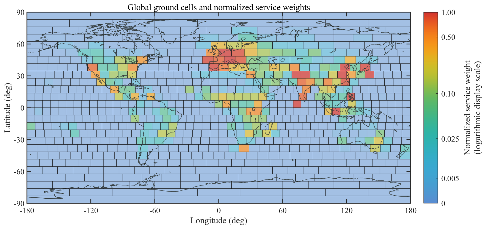
The global service region is discretized into approximately equal-area ground cells. The normalized service weight ${\omega }_q$ combines a baseline term, population density, terrestrial base-station density, and remote-region compensation. Figure 1 shows the resulting ground cells and their spatial weights. This model gives higher weights to demand-intensive regions while retaining nonzero weights in sparsely populated areas.

The best-link achievable-rate and positioning metrics are evaluated using the same satellite–ground visibility and link-budget data. The bandwidth and transmit-power values in Table 3 are applied independently to each evaluated ground-cell link; they do not represent simultaneous multi-cell resource allocation. At each epoch, each ground cell selects the serviceable satellite with the largest achievable rate. For Doppler positioning, visible satellites that satisfy the ${(C/N_0)}_{\mathrm{meas}}$ threshold under the selected service-beam direction enter the observation-window screening, subject to the observability and conditioning criteria defined in Section 2.5.

The parameters ${\kappa }_f$, $T_{\mathrm{int}}$, and ${\sigma }_{f,\mathrm{floor}}^2$ are signal- and receiver-specific because they depend on the waveform, frequency estimator, integration strategy, and receiver hardware, whereas ${\sigma }_{\mathrm{mp}}^2\left({\theta }_{qk,m}\right)$ is environment-specific. These components are therefore not instantiated separately in the reported numerical experiments. Instead, the overall conditional pseudo-range-rate measurement noise is represented by the fixed standard deviation ${\sigma }_{qk,m}={\sigma }_D=0.5\mathrm{m}/\mathrm{s}$, following the fixed Doppler-noise setting in [45]. Consequently, $C/N_0$ is used only to determine whether a Doppler observation is admitted and does not generate link-specific measurement variances in the reported simulations.

4.2. Validation of the Doppler Positioning Metric

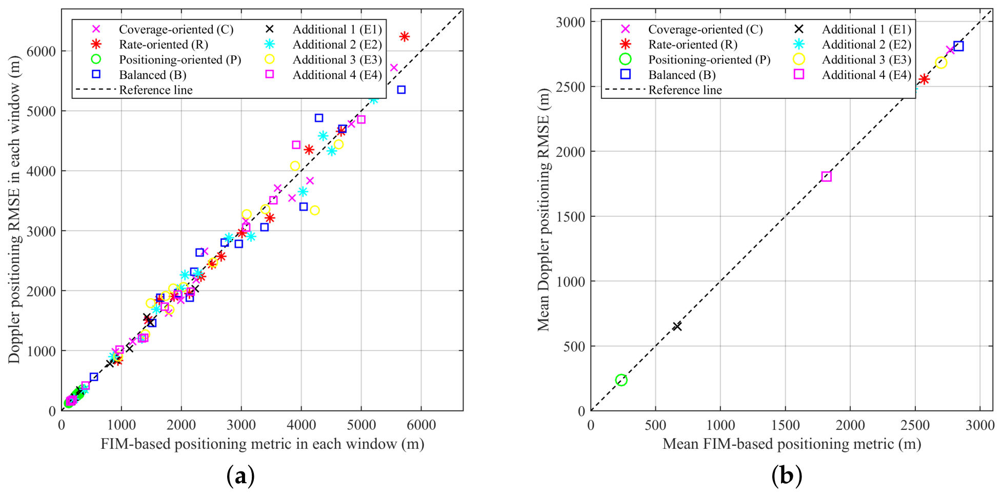
The SoP positioning objective $g_{\mathrm{pos}}\left(Y\right)$ is derived from the Fisher information matrix rather than computed with a receiver-level nonlinear Doppler positioning solver. This formulation is computationally efficient for constellation-level optimization because it avoids executing a full positioning algorithm for every candidate configuration. Its consistency with receiver-level positioning errors is examined under the simulation setting used for the optimization case with $N_{\mathrm{total}}=2000$.

Eight feasible dual-layer constellations are selected from the Pareto archive. They include the C, R, P, and B configurations and four additional configurations spanning intermediate regions of the feasible archive. For each constellation, 60 valid positioning windows are extracted according to the observability, link-quality, and conditioning criteria used to define ${\mathcal{W}}_q\left(Y\right)$. In each window, ${\epsilon }_q(\tau ;Y)$ is compared with the RMSE produced by a separately implemented multi-epoch nonlinear least-squares Doppler solver that jointly estimates the receiver position and nuisance states. Each RMSE is computed from 100 Monte Carlo noise realizations, giving 480 windows and 48,000 positioning trials in total. Both the FIM calculation and the Monte Carlo solver use the same observation model and the fixed-noise assumption ${\sigma }_D=0.5\mathrm{m}/\mathrm{s}$. This matched-model experiment is therefore a simulation-based consistency check rather than an independent physical validation.

Figure 2 presents the results at the window and configuration levels. At the window level, the FIM metric and Monte Carlo RMSE have a Pearson correlation coefficient of $0.9939$, a regression slope of $0.9953$, and a mean absolute percentage difference of $5.28\%$. After the 60 windows are averaged for each configuration, the corresponding values are $0.9999$, $0.9996$, and $0.76\%$, respectively. All nonlinear positioning trials converged. The validation is performed at the highest-weight ground cell; therefore, the configuration-level means in Figure 2b are local validation quantities rather than the globally aggregated objective $g_{\mathrm{pos}}\left(Y\right)$.

Under the adopted matched model, the FIM-based metric reproduces both the window-level error trend and the relative performance of the tested constellation configurations. These results support its use as a computationally efficient positioning objective for the constellation-level optimization considered here.

4.3. Sensitivity to Evaluation Thresholds

The local sensitivity of the reported metrics to ${(C/N_0)}_{\mathrm{meas}}$ and ${\mathsf{\Gamma }}_{\mathrm{srv}}$ is evaluated using the fixed C, R, P, and B configurations. Each threshold is varied separately around its baseline value without re-optimizing the constellations.

Table 4. Sensitivity of representative configurations to the Doppler and communication thresholds.

Threshold Setting	$\mathsf{\Delta }{\mathit{f}}_{\mathbf{cov}}$ (Percentage Points)	$\mathsf{\Delta }{\mathit{f}}_{\mathbf{com}}$ (%)	$\mathsf{\Delta }{\mathit{g}}_{\mathbf{pos}}$ (%)	$\mathsf{\Delta }{\mathit{a}}_{\mathbf{pos}}$ (Percentage Points)	Feasible Cases
${(C/N_0)}_{\mathrm{meas}}=33\mathrm{dB}\mathrm{Hz}$	0	0	$-32.9$ to $-16.0$	$+0.04$ to $+0.43$	$4/4$
${(C/N_0)}_{\mathrm{meas}}=37\mathrm{dB}\mathrm{Hz}$	0	0	$+22.1$ to $+166.0$	$-0.43$ to $-0.03$	$3/4$
${\mathsf{\Gamma }}_{\mathrm{srv}}=3\mathrm{dB}$	$+0.83$ to $+2.59$	$+0.26$ to $+0.84$	$-23.0$ to $+4.1$	$+0.64$ to $+1.44$	$4/4$
${\mathsf{\Gamma }}_{\mathrm{srv}}=7\mathrm{dB}$	$-4.01$ to $-2.53$	$-1.66$ to $-0.99$	$-16.7$ to $+6.7$	$-2.81$ to $-1.99$	$0/4$

reports the range of changes across the four configurations. The feasibility count uses the baseline requirement $a_{\mathrm{pos}}\left(Y\right)\ge 0.98$.

Changing ${(C/N_0)}_{\mathrm{meas}}$ leaves $f_{\mathrm{cov}}$ and $f_{\mathrm{com}}$ unchanged because this threshold screens only Doppler observations. A lower threshold admits more observations and reduces $g_{\mathrm{pos}}$ by $16.0$–$32.9\%$, whereas a threshold of $37\mathrm{dB}\mathrm{Hz}$ increases $g_{\mathrm{pos}}$ by $22.1$–$166.0\%$ and makes configuration P infeasible. In the adopted model, changing ${\mathsf{\Gamma }}_{\mathrm{srv}}$ modifies service-link availability and the selected receiver boresight, thereby indirectly changing the positioning-observation set and geometry. All four configurations remain feasible at $3\mathrm{dB}$, whereas none meets $a_{\mathrm{pos}}\left(Y\right)\ge 0.98$ at $7\mathrm{dB}$. Because $g_{\mathrm{pos}}$ is averaged over the valid-window set ${\mathcal{W}}_q\left(Y\right)$, which also varies with the thresholds, its aggregate response need not be monotonic.

A retention analysis is also performed on the 73 Pareto configurations generated with $a_{min}=0.980$. Applying $a_{min}=0.985$ and $0.990$ retains 44 and 12 configurations, respectively; neither case involves re-optimization. These results show how the feasibility of the reported Pareto set depends on the adopted thresholds.

4.4. Pareto Optimization Results and Positioning-Objective Ablation

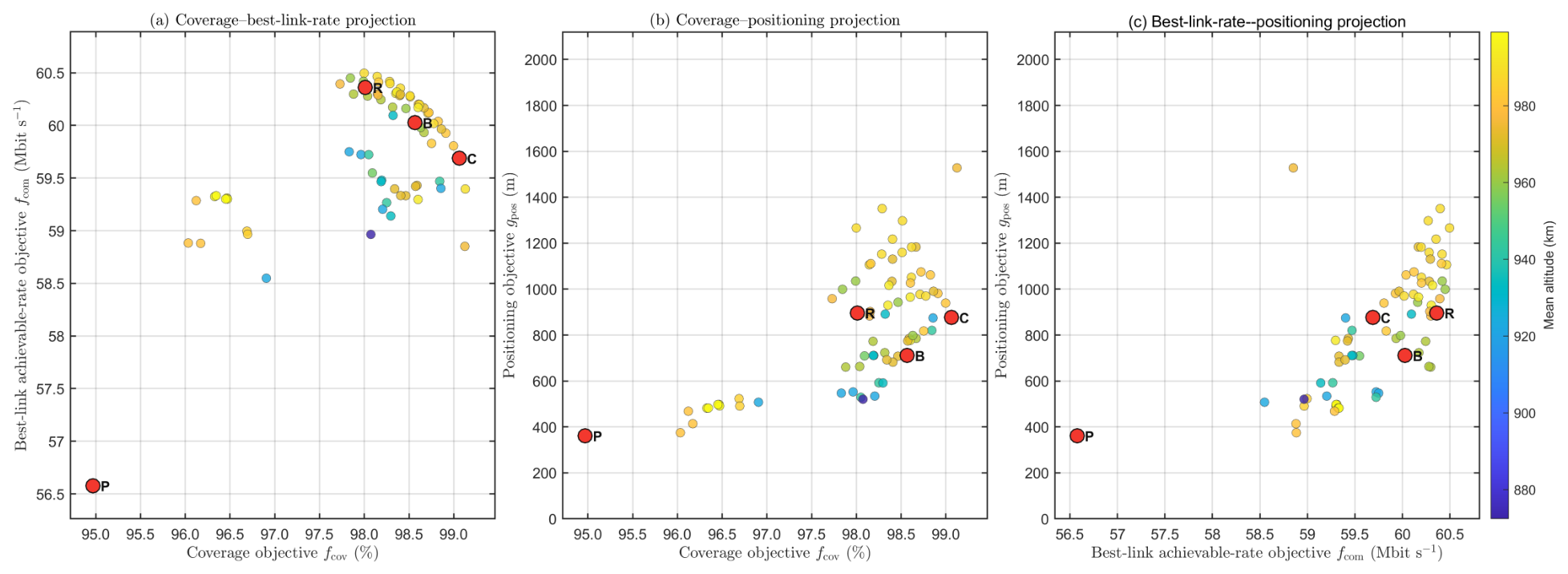
This subsection reports the Pareto archive obtained by the proposed CMI-MOAHA method and evaluates the effect of explicitly including the SoP positioning objective. The case with $N_{\mathrm{total}}=2000$ is used as the main optimization scenario. This constellation scale provides broad global service while retaining non-trivial trade-offs among coverage, best-link achievable rate, and Doppler positioning performance. The final feasible archive contains 73 dual-layer configurations. The weighted coverage objective ranges from $94.97\%$ to $99.13\%$, and the best-link achievable-rate objective ranges from $56.58\mathrm{Mbit}/\mathrm{s}$ to $60.50\mathrm{Mbit}/\mathrm{s}$. The smallest positioning objective is $361.4\mathrm{m}$. All feasible configurations satisfy $a_{\mathrm{pos}}\left(Y\right)\ge 0.98$, with $a_{\mathrm{pos}}\left(Y\right)$ ranging from $98.0\%$ to $99.5\%$.

Figure 3 shows the pairwise projections of the feasible archive. Each point represents one dual-layer constellation configuration, and the color indicates the mean constellation altitude. The four highlighted configurations denote coverage-oriented (C), rate-oriented (R), positioning-oriented (P), and balanced (B) solutions. The balanced solution B is selected according to the normalized objectives $f_{\mathrm{cov}}\left(Y\right)$, $f_{\mathrm{com}}\left(Y\right)$, and $-g_{\mathrm{pos}}\left(Y\right)$.

The Pareto projections indicate that the three objectives are coupled but not interchangeable. The positioning-oriented region favors a different altitude–inclination allocation and achieves a substantially lower $g_{\mathrm{pos}}\left(Y\right)$, whereas the coverage- and rate-oriented configurations retain stronger service metrics. The archive therefore exhibits a clear trade-off between service and positioning performance, with no single metric dominating the others.

Table 5. Representative configurations selected from the feasible Pareto archive for the dual-layer constellation case with $N_{\mathrm{total}}=2000$.

Label	Preference	Layer 1	Layer 2	${\mathit{f}}_{\mathbf{cov}}$ (%)	${\mathit{f}}_{\mathbf{com}}$ (Mbit/s)	${\mathit{g}}_{\mathbf{pos}}$ (m)	${\mathit{a}}_{\mathbf{pos}}$ (%)
C	Coverage	$(900,31.5,37\times 32,1184)$	$(1100,79.5,24\times 34,816)$	99.1	59.69	877.0	99.3
R	Best-link achievable rate	$(800,34.5,36\times 31,1116)$	$(1200,80.0,26\times 34,884)$	98.0	60.36	896.0	98.2
P	Positioning	$(650,78.0,28\times 28,784)$	$(1100,36.5,38\times 32,1216)$	95.0	56.58	361.4	98.3
B	Balanced	$(800,33.0,37\times 32,1184)$	$(1200,79.5,24\times 34,816)$	98.6	60.03	711.5	98.8

reports the orbital parameters and performance metrics of the four highlighted configurations.

Configurations C and R emphasize service coverage and best-link achievable rate, respectively, while both keep the positioning metric below $900\mathrm{m}$. Configuration P gives the smallest positioning objective, $g_{\mathrm{pos}}=361.4\mathrm{m}$, but its coverage and best-link achievable-rate objectives decrease to $95.0\%$ and $56.58\mathrm{Mbit}/\mathrm{s}$. Configuration B provides a more balanced operating point. Compared with R, B reduces the positioning metric by about $20.6\%$, while $f_{\mathrm{com}}\left(Y\right)$ decreases by only $0.33\mathrm{Mbit}/\mathrm{s}$. This comparison shows that the FIM-based positioning metric can be substantially improved near the rate-oriented region with only a limited reduction in the best-link achievable-rate objective.

The smallest FIM-based value, $g_{\mathrm{pos}}=361.4\mathrm{m}$, is of the same order of magnitude as results reported in several LEO Doppler SoP studies. Carrier-Doppler positioning using Iridium, Orbcomm, and Starlink signals has been reported on the order of ${10}^2\mathrm{m}$ [26]. Historical TRANSIT fixes achieved an accuracy of approximately $200\mathrm{m}$ [22], and a two-satellite ORBCOMM experiment reported a horizontal positioning error of $358\mathrm{m}$ [24]. Numerical investigations also show that the attainable error can range from tens to hundreds of meters across different LEO constellations under a range-rate measurement noise of $0.1\mathrm{m}/\mathrm{s}$ [23]. However, this value is a model-conditioned position-error lower-bound metric rather than a prediction of field accuracy. Satellite-specific clock and ephemeris errors, atmospheric propagation errors, multipath, and receiver implementation effects are not fully represented. The literature values therefore provide only order-of-magnitude context for the reported metric.

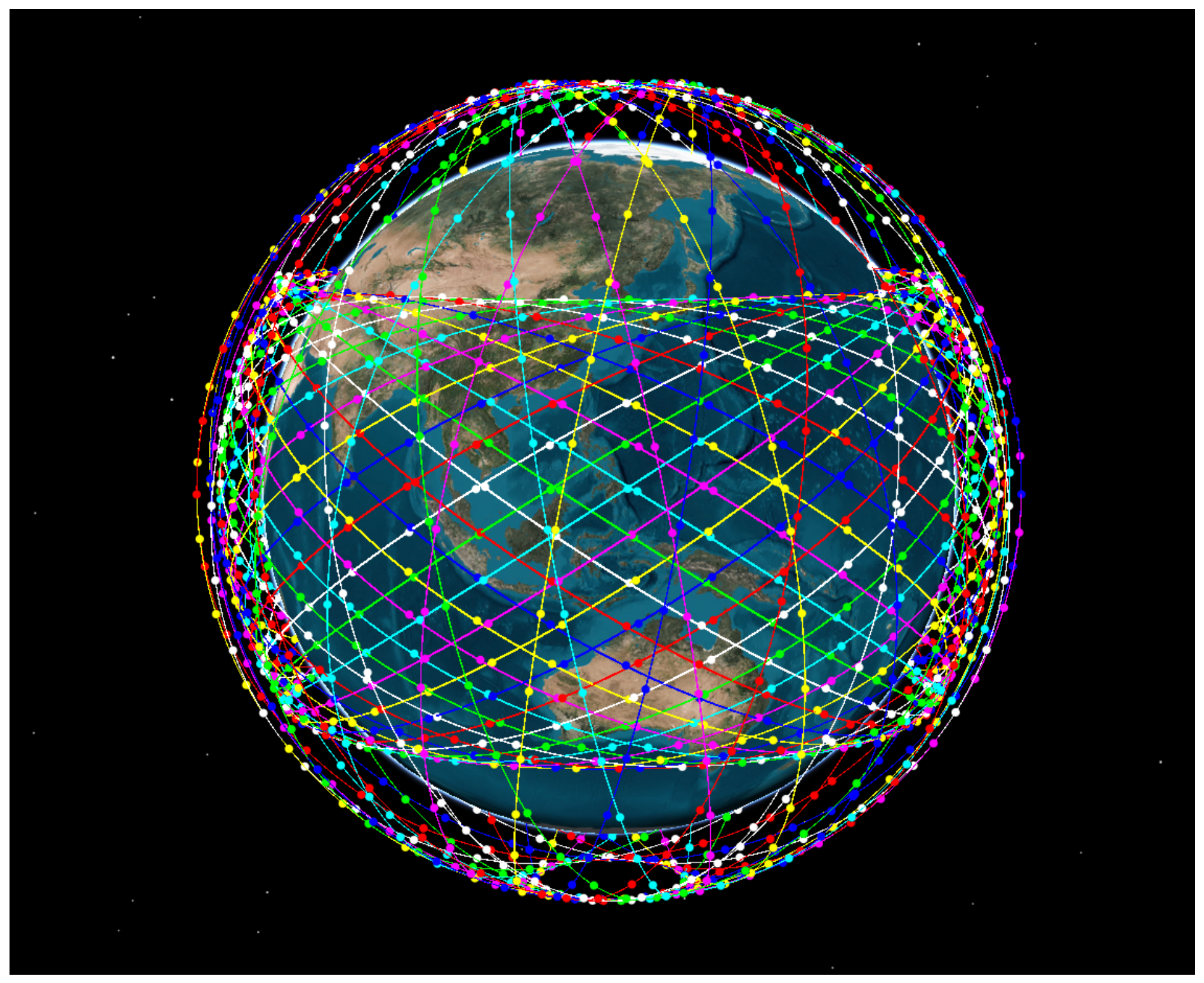
The visualization of the balanced 2000-satellite constellation configuration is shown in Figure 4.

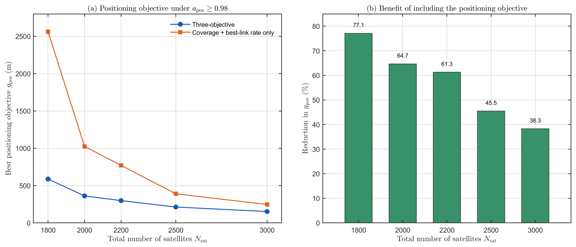
To examine the role of the positioning objective, the proposed three-objective optimization is compared with a two-objective optimization of coverage and best-link achievable rate. The comparison is performed for different total numbers of satellites. In the two-objective case, $g_{\mathrm{pos}}\left(Y\right)$ is not used during the search and is evaluated only after the candidate constellations are obtained. Only configurations satisfying $a_{\mathrm{pos}}\left(Y\right)\ge 0.98$ are included.

The ablation results in Figure 5 show that explicitly including the positioning objective reduces the best obtained $g_{\mathrm{pos}}\left(Y\right)$ across all tested values of $N_{\mathrm{total}}$. The largest reduction occurs when $N_{\mathrm{total}}=1800$, for which the best $g_{\mathrm{pos}}\left(Y\right)$ decreases from $2562.0\mathrm{m}$ to $587.7\mathrm{m}$, corresponding to a $77.1\%$ reduction. For $N_{\mathrm{total}}=2000$, the best $g_{\mathrm{pos}}\left(Y\right)$ in the main 2000-satellite Pareto archive decreases from $1023.9\mathrm{m}$ in the coverage-and-best-link-rate-only optimization to $361.4\mathrm{m}$ when the positioning objective is included, corresponding to a $64.7\%$ reduction.

The relative reduction decreases with $N_{\mathrm{total}}$ over the tested range but remains substantial. When $N_{\mathrm{total}}=3000$, the best positioning objective decreases from $246.7\mathrm{m}$ to $152.1\mathrm{m}$, giving a $38.3\%$ reduction. As the constellation becomes denser, improved visibility and link availability can also benefit Doppler positioning. However, the coverage and best-link achievable-rate objectives do not directly minimize the position-error bound. The explicit positioning objective therefore remains important for identifying positioning-favorable Pareto solutions, especially when the total number of satellites is limited.

Table 6. Configuration-wise paired results of the three-objective and coverage-and-best-link-rate-only optimizations under different total satellite numbers. Each row reports the orbital parameters and performance metrics of one specific feasible configuration. The layer tuple is $(h_l,i_l,P_l\times S_l,N_{\mathrm{sat}}^{\left(l\right)})$.

${\mathit{N}}_{\mathbf{total}}$	Optimization Objectives	Layer 1	Layer 2	${\mathit{f}}_{\mathbf{cov}}$(%)	${\mathit{f}}_{\mathbf{com}}$(Mbit/s)	${\mathit{g}}_{\mathbf{pos}}$(m)	${\mathit{a}}_{\mathbf{pos}}$(%)
1800	Three-objective	$(900,33.0,36\times 32,1152)$	$(1150,78.5,27\times 24,648)$	95.1	55.60	587.7	98.5
	Coverage + best-link rate	$(850,32.5,35\times 30,1050)$	$(1150,78.0,15\times 50,750)$	98.6	57.60	2562.0	98.4
2000	Three-objective	$(650,78.0,28\times 28,784)$	$(1100,36.5,38\times 32,1216)$	95.0	56.58	361.4	98.3
	Coverage + best-link rate	$(900,30.0,37\times 32,1184)$	$(1100,79.0,34\times 24,816)$	98.9	58.59	1023.9	99.5
2200	Three-objective	$(800,77.5,32\times 35,1120)$	$(1000,35.5,36\times 30,1080)$	95.2	59.70	298.4	98.0
	Coverage + best-link rate	$(850,33.5,35\times 30,1050)$	$(1100,79.5,25\times 46,1150)$	98.5	61.86	770.6	99.0
2500	Three-objective	$(750,42.0,44\times 32,1408)$	$(1150,77.5,28\times 39,1092)$	96.5	62.53	212.5	98.3
	Coverage + best-link rate	$(900,36.5,43\times 36,1548)$	$(1150,79.5,28\times 34,952)$	99.3	63.35	389.7	99.6
3000	Three-objective	$(550,46.5,56\times 33,1848)$	$(950,80.0,32\times 36,1152)$	97.0	65.00	152.1	98.1
	Coverage + best-link rate	$(800,33.0,40\times 35,1400)$	$(1000,80.0,32\times 50,1600)$	99.4	66.49	246.7	99.6

complements the best-value comparison by reporting the orbital parameters and performance metrics of representative feasible configurations for the two formulations at each tested constellation size.

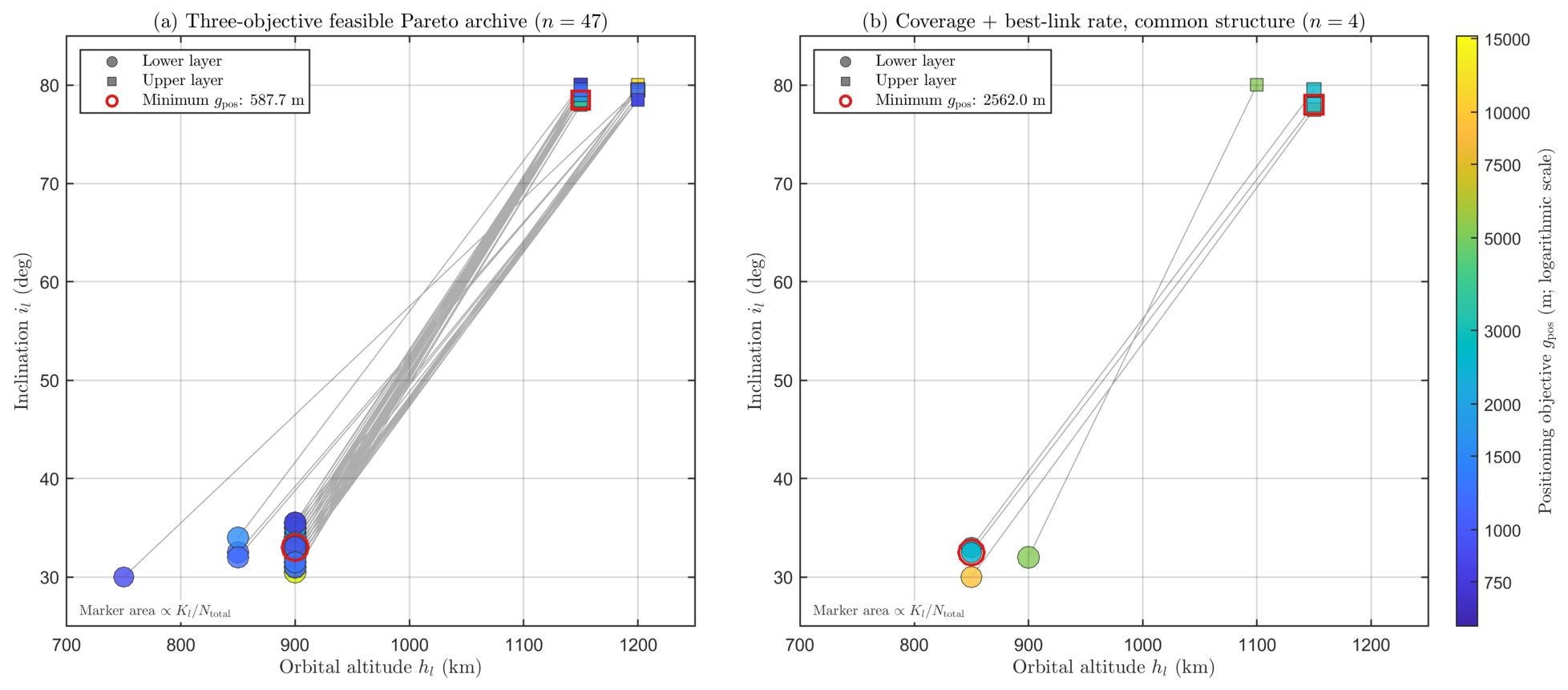
To examine the orbital characteristics associated with the largest reduction, Figure 6 compares the 47 configurations in the three-objective feasible Pareto archive with the four positioning-feasible two-objective configurations that share the same broad altitude–inclination structure.

The two displayed sets of configurations exhibit a similar broad structure. In the three-objective archive, the lower layer lies at 750–$900\mathrm{km}$ with inclinations of $30.0^{\circ }$–$35.5^{\circ }$, while the upper layer lies at 1150–$1200\mathrm{km}$ with inclinations of $78.0^{\circ }$–$80.0^{\circ }$. The four two-objective configurations place the lower layer at 850–$900\mathrm{km}$ and $30.0^{\circ }$–$33.0^{\circ }$, and the upper layer at 1100–$1150\mathrm{km}$ and $77.5^{\circ }$–$80.0^{\circ }$. This common altitude–inclination organization is therefore favored by both formulations and is not, by itself, a distinctive effect of the positioning objective.

The main observed difference lies in the near-polar layer allocation. The three-objective archive uses 21–30 near-polar orbital planes and places 23–30 satellites in each plane. The four two-objective configurations use 15–21 near-polar planes and place 26–50 satellites in each plane. Thus, the positioning-oriented solutions distribute the near-polar population over more orbital planes rather than concentrating more satellites within each plane. This pattern provides a configuration-level explanation for the positioning gain without attributing it to a single altitude or inclination value.

4.5. Single-Initialization Paired Benchmark Against NSGA-II

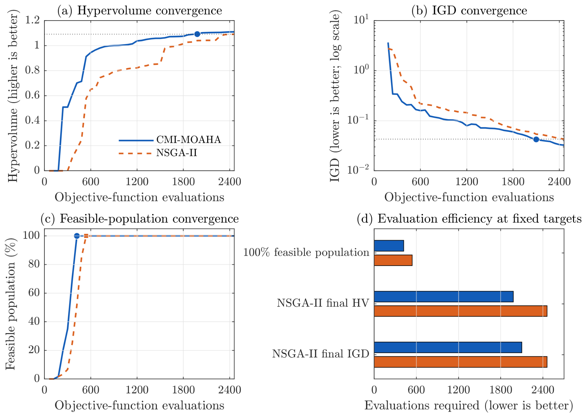
For the single tested initialization, CMI-MOAHA is compared with a constrained mixed-integer NSGA-II baseline in a paired run under the main 2000-satellite scenario. Both algorithms start from the same 60 repaired constellation designs and use $N_{\mathrm{pop}}=60$, $G_{max}=40$, $N_{\mathcal{A}}=160$, random seed 71, and exactly 2460 objective-function evaluations; evaluation caching is disabled. The NSGA-II baseline uses binary tournament selection, simulated-binary crossover with a probability of 0.90 and a distribution index of 20, and polynomial mutation with probability $1/n_{\mathrm{var}}$ and a distribution index of 20. Both methods share the constellation encoding, feasibility mapping $\mathsf{\Pi }(·)$, objectives, constraints, and simulation evaluator. For hypervolume (HV) and inverted generational distance (IGD), the objective values are normalized over the union of the final feasible archives. The empirical non-dominated union serves as the IGD reference front, and the normalized HV reference point is $(1.10,1.10,1.10)$ [46]. A larger HV and a smaller IGD indicate better aggregate Pareto-search quality.

As shown in Figure 7, the final HV for this single paired run is $1.10991$ for CMI-MOAHA and $1.09133$ for NSGA-II, corresponding to a $1.70\%$ increase. The final CMI-MOAHA IGD is $0.032464$, which is $24.01\%$ lower than the NSGA-II value of $0.042722$. The two populations reach full feasibility after 420 and 540 evaluations, respectively; thus, CMI-MOAHA requires $22.2\%$ fewer evaluations in this run. CMI-MOAHA also reaches the final NSGA-II HV and IGD after 1980 and 2100 evaluations, respectively, corresponding to $19.5\%$ and $14.6\%$ fewer evaluations than the full 2460-evaluation budget. To exclude startup and initial-evaluation overhead from the runtime comparison, wall-clock runtime is accumulated after generation 3. The corresponding values are $5391.1\mathrm{s}$ for CMI-MOAHA and $5339.4\mathrm{s}$ for NSGA-II, indicating comparable post-initialization costs for this run. For this initialization, CMI-MOAHA reaches a fully feasible population earlier and produces a higher final HV and a lower final IGD at a similar post-initialization runtime. Independent runs are needed to assess stochastic variability and determine whether these differences persist.

4.6. Comparison Between Optimized Dual-Layer and Single-Layer Constellations

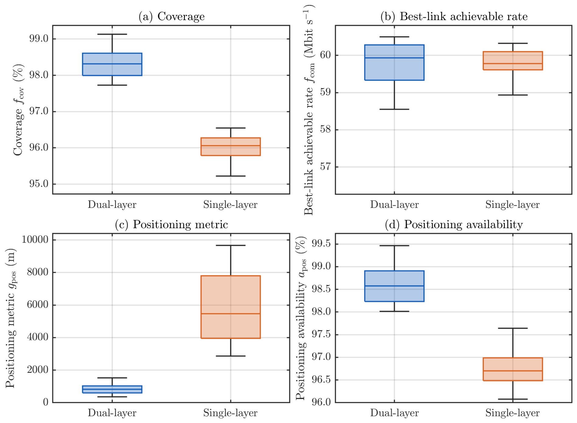
To examine the effect of constellation architecture, the dual-layer constellation is compared with a single-layer Walker constellation under the same total number of satellites and evaluation model. Both cases use $N_{\mathrm{total}}=2000$, and the formal feasibility criterion $a_{\mathrm{pos}}\left(Y\right)\ge 0.98$ is applied consistently. The single-layer architecture places all satellites in one orbital shell, whereas the dual-layer architecture distributes them between two independently configured Walker layers.

The dual-layer search produces 73 configurations satisfying the formal positioning-availability criterion. In contrast, no candidate returned by the single-layer search satisfies $a_{\mathrm{pos}}\left(Y\right)\ge 0.98$. Figure 8 therefore compares the feasible dual-layer archive with a diagnostic single-layer population. The latter is retained to quantify the performance shortfall but is not treated as a feasible solution set. The two distributions have similar $f_{\mathrm{com}}\left(Y\right)$ ranges, whereas the dual-layer archive achieves higher coverage and substantially smaller $g_{\mathrm{pos}}\left(Y\right)$. Its positioning availability remains above $98.0\%$, while all single-layer candidates remain below the required threshold.

Table 7. Configuration-wise performance of the dual-layer feasible solution and the single-layer diagnostic candidate for the $N_{\mathrm{total}}=2000$ case.

Architecture	Status	Configuration	${\mathit{f}}_{\mathbf{cov}}$(%)	${\mathit{f}}_{\mathbf{com}}$(Mbit/s)	${\mathit{g}}_{\mathbf{pos}}$(m)	${\mathit{a}}_{\mathbf{pos}}$(%)
Dual-layer	Feasible	L1: $(650,78.0,28\times 28,784)$	95.0	56.58	361.4	98.3
		L2: $(1100,36.5,38\times 32,1216)$
Single-layer	Infeasible diagnostic	$(1200,75.0,50\times 40,2000)$	96.1	59.52	2867.7	97.0

reports configuration-wise metrics for two positioning-oriented candidates: the best-positioning feasible dual-layer configuration and the best-positioning candidate in the diagnostic single-layer population. All four metrics in each row are evaluated for the same constellation configuration, and the feasibility status is stated explicitly.

The architecture comparison shows that layer allocation provides additional freedom to jointly shape service continuity and Doppler observation geometry. The diagnostic single-layer candidate retains a comparable best-link achievable-rate value, but its positioning availability is below the formal requirement and its $g_{\mathrm{pos}}\left(Y\right)$ is substantially larger. Within the examined design space and search setting, only the dual-layer search returned configurations satisfying the formal feasibility criterion. This finding does not imply that every single-layer constellation is incapable of meeting the positioning-availability requirement.

4.7. Comparison with Reference Constellation Designs

Three published reference cases are considered. Sun-TNSM denotes the user-distribution-oriented Walker-Delta configuration in [10], while PA-ICD-r and PA-ICD-DL denote the r-priority single-layer and dual-layer configurations in [41], respectively.

The proposed constellation corresponds to solution B in Table 5. The reference constellation designs retain the orbital parameters reported in the corresponding studies and are not re-optimized under the proposed objective functions. The notation $h_l/i_l/P_l\times S_l/N_{\mathrm{sat}}^{\left(l\right)}$ is used to describe each layer, where $h_l$ is the orbital altitude, $i_l$ is the inclination, $P_l$ is the number of orbital planes, $S_l$ is the number of satellites per plane, and $N_{\mathrm{sat}}^{\left(l\right)}=P_l{S}_l$ is the number of satellites in that layer. All cases are evaluated using the same ground grid, link-budget model, time sampling, Doppler observation-window setting, and positioning-availability criterion. Because the total satellite numbers differ, this analysis compares the reference designs under a common evaluation model but does not constitute a controlled comparison at equal constellation size.

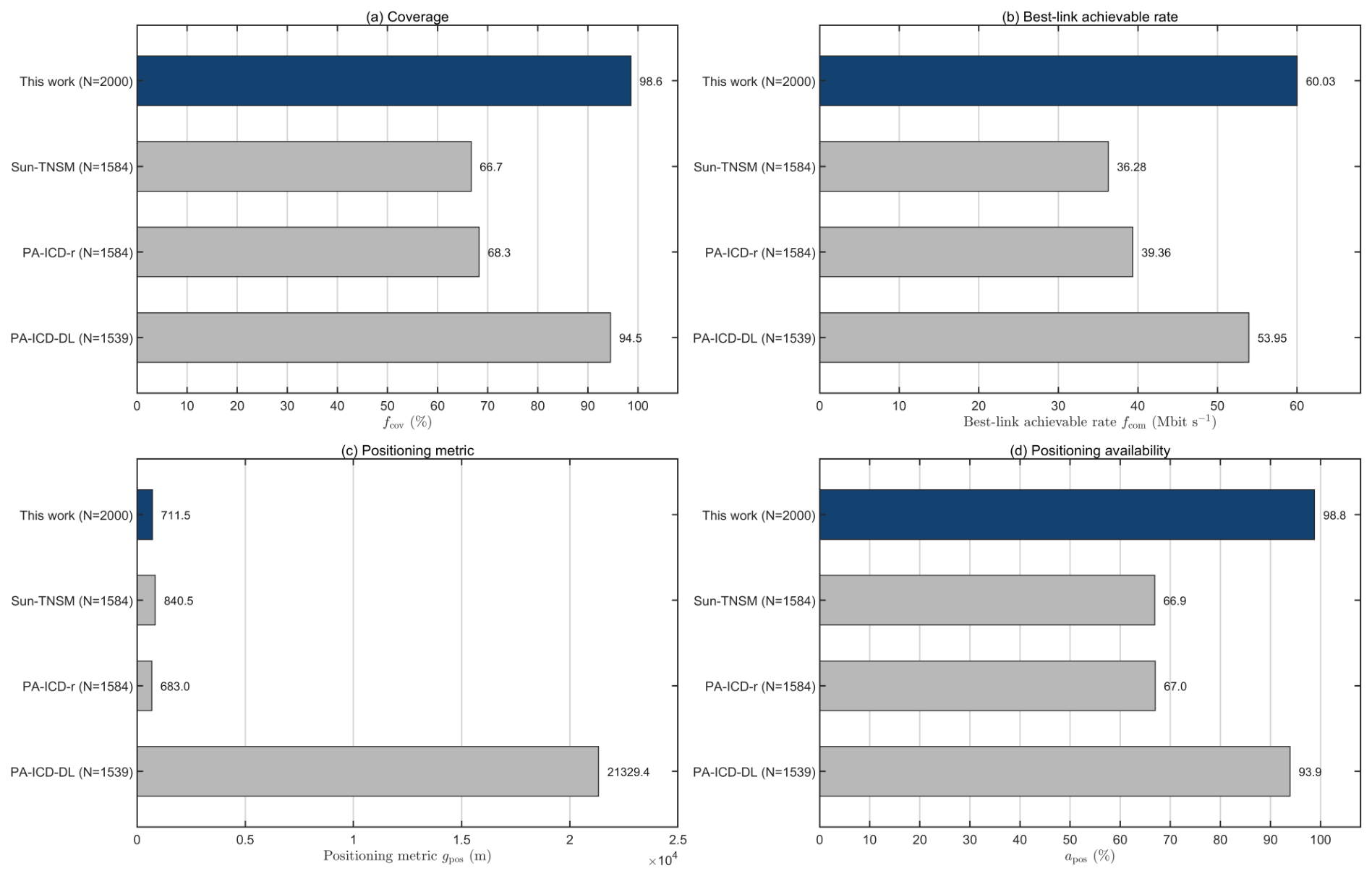
Figure 9 compares the four cases in terms of coverage, best-link achievable rate, the FIM-based positioning metric, and positioning availability. The proposed constellation achieves $98.6\%$ coverage, a best-link achievable-rate value of $60.03\mathrm{Mbit}/\mathrm{s}$, $g_{\mathrm{pos}}\left(Y\right)=711.5\mathrm{m}$, and $98.8\%$ positioning availability. Under the adopted evaluation model, it gives the highest $f_{\mathrm{cov}}\left(Y\right)$, $f_{\mathrm{com}}\left(Y\right)$, and $a_{\mathrm{pos}}\left(Y\right)$ values among the four cases. PA-ICD-r gives a slightly smaller $g_{\mathrm{pos}}\left(Y\right)$ of $683.0\mathrm{m}$, so no single case is best in all four metrics.

The numerical results are summarized in

Table 8. Performance comparison between the proposed balanced constellation and reference constellation designs.

Case	${\mathit{N}}_{\mathbf{sat}}$	Configuration	Mean alt.(km)	${\mathit{f}}_{\mathbf{cov}}$(%)	${\mathit{f}}_{\mathbf{com}}$(Mbit/s)	${\mathit{g}}_{\mathbf{pos}}$(m)	${\mathit{a}}_{\mathbf{pos}}$(%)
Proposed-B	2000	L1: $800/33.0/37\times 32/1184$;	963.2	98.6	60.03	711.5	98.8
		L2: $1200/79.5/24\times 34/816$
Sun-TNSM	1584	$1150/36.0/72\times 22/1584$	1150.0	66.7	36.28	840.5	66.9
PA-ICD-r	1584	$620/43.0/72\times 22/1584$	620.0	68.3	39.36	683.0	67.0
PA-ICD-DL	1539	L1: $1015/76.0/9\times 37/333$;	1257.9	94.5	53.95	21,329.4	93.9
		L2: $1325/44.0/18\times 67/1206$

. Sun-TNSM and PA-ICD-r provide about 67–$68\%$ weighted coverage and positioning availability under the adopted global service model. PA-ICD-r gives a slightly smaller $g_{\mathrm{pos}}\left(Y\right)$ than the proposed solution but substantially lower service continuity. PA-ICD-DL provides higher coverage and a larger $f_{\mathrm{com}}\left(Y\right)$ value than the single-layer reference cases, with $94.5\%$ coverage and $f_{\mathrm{com}}\left(Y\right)=53.95\mathrm{Mbit}/\mathrm{s}$. However, its positioning metric is much larger, indicating that a multi-layer architecture alone does not ensure favorable SoP positioning geometry.

Taken together, the comparison places the proposed balanced solution within the service–positioning trade-offs represented by the published constellation designs. The proposed solution combines high service continuity and best-link achievable rate with $98.8\%$ positioning availability, whereas PA-ICD-r attains a slightly smaller positioning metric at substantially lower coverage and availability. The reference cases use different satellite numbers and retain the configurations reported in their original studies. The results should therefore be interpreted as a descriptive comparison under a common evaluation model rather than as a controlled benchmark of the proposed optimization method. They further suggest that constellation designs developed for coverage- or computing-oriented objectives should be re-evaluated or re-optimized before being applied to an integrated communication and SoP positioning task.

5. Conclusions

This paper presented a multi-layer LEO constellation optimization framework for integrated communication and SoP Doppler positioning. Weighted service coverage, weighted best-link achievable rate, and Doppler positioning performance were modeled under a unified satellite–ground geometry and link-budget setting. A link-quality-constrained multi-epoch FIM metric was introduced for constellation-level positioning evaluation. The resulting constrained mixed-integer multi-objective problem was solved using CMI-MOAHA to generate constrained non-dominated constellation configurations.

The matched-model comparison showed that the proposed positioning metric closely tracks the Monte Carlo RMSE from a separately implemented nonlinear Doppler positioning solver, supporting its use as an efficient optimization objective under the adopted assumptions. For $N_{\mathrm{total}}=2000$, the feasible Pareto archive revealed clear trade-offs among coverage, best-link achievable rate, and Doppler positioning performance. The ablation results showed that including the positioning objective guides the search toward configurations with more favorable SoP geometry. Within the examined design space and search setting, only the dual-layer search returned configurations satisfying the formal positioning-availability criterion. The diagnostic single-layer population retained a comparable $f_{\mathrm{com}}\left(Y\right)$ range but had lower positioning availability and poorer positioning performance.

The descriptive comparison with reference constellation designs suggests that coverage- or rate-oriented configurations may require re-evaluation or re-optimization before being applied to the integrated service-positioning problem. However, the reference cases use different satellite numbers and retain their originally reported configurations, so the comparison is not a controlled benchmark of the proposed optimization method. Overall, the results support joint optimization of coverage, best-link achievable rate, and link-quality-constrained Doppler positioning when LEO communication satellites also serve as SoP for Doppler positioning.

The best-link achievable-rate objective isolates geometry-dependent rate potential under a common reference link budget rather than aggregate network throughput, while the FIM-based positioning metric is a model-conditioned position-error lower bound rather than a prediction of field accuracy. The reported results apply to nominal noise-limited, non-jammed conditions. The separation of orbital propagation from performance evaluation allows more detailed communication-performance models to be incorporated without changing the Walker constellation representation and orbital-propagation model. Existing studies have considered shared bandwidth and co-channel interference [8], SINR-based rates and differentiated QoS requirements [12], and topology- and traffic-aware interference [13]. Future work will incorporate these elements, together with beam and resource allocation, feeder-link constraints, and dynamic traffic demand, and compare the constellation configurations obtained by re-optimization under different communication assumptions. Further extensions will consider intentional interference, jamming-aware link availability, robust Doppler processing, inter-satellite networking, and refined clock and orbit error models. Future work will also benchmark additional constrained multi-objective methods over multiple independent initializations and integrate constellation configuration with self-organized network control and cross-layer in-space computation offloading.