1. Introduction
Software defect prediction is an important software quality assurance activity that aims to identify software entities that are likely to contain defects before testing, inspection, and maintenance resources are allocated. Reliable defect prediction can help practitioners prioritize limited verification effort, focus code review on high-risk components, and reduce the cost of late defect discovery. At class level, defect prediction is commonly formulated as a binary classification task in which each class is labeled as defective or clean based on historical defect information. This granularity is particularly relevant for object-oriented systems because classes are central units of design, implementation, testing, and maintenance.
Traditional class-level defect prediction has relied heavily on static software metrics that summarize structural properties of software entities, such as size, complexity, coupling, cohesion, inheritance, and documentation. Object-oriented metrics, including the Chidamber and Kemerer metric suite, have been widely used because they provide interpretable indicators of structural quality and fault-proneness [
1]. Several empirical studies and benchmarks have shown that such metrics can be useful predictors of defects and that rigorous comparative evaluation is essential when assessing defect-prediction models [
2,
3,
4,
5,
6,
7]. From a software quality perspective, these metrics remain important not only because they are easy to compute and interpret, but also because they provide strong baselines for evaluating whether newer learned representations add practical predictive value.
Recent advances in machine learning for software engineering, particularly deep learning and pre-trained code representation learning, have created new opportunities for defect prediction. Deep learning-based defect prediction has been increasingly studied in empirical software engineering, with recent reviews highlighting both its promise and its methodological challenges, including dataset selection, prediction granularity, class imbalance, validation protocol, and baseline choice [
8,
9,
10]. Pre-trained code models such as CodeBERT, GraphCodeBERT, CodeT5, and UniXcoder learn dense representations of source code from large corpora and can be adapted to downstream software engineering tasks [
11,
12,
13,
14]. Because these models encode lexical, syntactic, and semantic information from source code, they are attractive for defect prediction, where researchers may wish to replace or complement manually designed software metrics with learned code representations.
However, the practical value of pre-trained code models for class-level defect prediction remains an open empirical question. In many studies, learned code representations are evaluated primarily in terms of predictive performance, while less attention is given to three methodological issues that are central for software quality prediction. First, class-level Java entities can be much longer than the effective input budget of common Transformer-based code encoders. If only the first window of tokens is retained, the resulting representation may exclude large parts of the class body. Second, input truncation may not be randomly distributed. If defective classes are more likely to be long and therefore more likely to overflow the model input budget, then truncation may disproportionately affect the instances that defect prediction models are intended to identify. Third, traditional metrics already capture several size- and structure-related factors associated with defect-proneness. Therefore, a pre-trained code model should not only perform well in isolation; it should also be evaluated for its incremental value beyond strong metric-based baselines and size controls.
These concerns are particularly important because recent defect-prediction studies have begun to use CodeBERT and related pre-trained representations directly. For example, Pan et al. evaluated CodeBERT-based models for software defect prediction [
15], Sahar et al. proposed a supervised contrastive learning approach using CodeBERT [
16], and Yang et al. proposed a CodeBERT-driven collaborative generative adversarial learning approach for defect prediction [
17]. Other recent studies have combined learned semantic or structural representations with traditional software features [
18,
19,
20]. These studies demonstrate the growing interest in learned code representations for software quality prediction. At the same time, they motivate a more direct empirical question: do pre-trained code models provide predictive value beyond established software metrics when input coverage, long-code representation, and chronological cross-version generalization are explicitly considered?
This paper investigates that question through a class-level empirical study of pre-trained code models for defect prediction. Rather than treating input truncation as a minor preprocessing detail, the study treats input coverage as a methodological validity issue. The central premise is that a learned representation cannot be assumed to be reliable if a large and label-dependent portion of the source code is excluded before representation learning. Similarly, a pre-trained code model cannot be assumed to improve software quality prediction unless its contribution is evaluated against strong metric baselines, size-only controls, and realistic cross-version splits.
The study evaluates three pre-trained code models: CodeBERT, GraphCodeBERT, and CodeT5. CodeBERT is included as a widely used reference model for programming language and natural language representation learning [
11]. GraphCodeBERT is included because it extends code representation learning by incorporating data-flow information [
12]. CodeT5 is included because it is an identifier-aware encoder–decoder model for code understanding and generation tasks [
13]. By evaluating more than one pre-trained code model, the study avoids drawing conclusions from a single encoder and allows input coverage and predictive value to be examined across different pre-training designs.
The study also evaluates multiple input-representation strategies. Truncation-based baselines include First-window, Last-window, and Head-tail representations. These baselines reflect common ways of forcing long classes into a fixed input budget. Long-code-aware strategies include simple split–encode–aggregate representations, such as chunk-mean and chunk-max pooling, and a lightweight trainable chunk-attention model. This design is motivated by prior long-code research showing that splitting, encoding, and aggregating code blocks can be a practical way to handle long code with existing pre-trained models [
21]. More specialized long-code architectures, such as LongCoder and Bridge and Hint, further demonstrate that long-code modeling is an active research problem [
22,
23]. In this study, however, the goal is not to propose a new long-code architecture. Instead, the goal is to test whether increasingly stronger input-coverage strategies actually improve class-level defect prediction and whether any improvement is large enough to matter beyond traditional metrics.
To support realistic evaluation, the study uses the class-level PROMISE subset of the Unified Bug Dataset [
24]. The dataset is cleaned through source-code mapping and filtering to retain production class-level instances and to remove anonymous, local, synthetic, generated, test-source, and empty-code entries. The final dataset contains 16,237 Java classes from six projects: Ant, Camel, JEdit, Lucene, Poi, and Synapse. Models are evaluated using 11 chronological cross-version train–validation–test splits; where earlier version(s) are used for training, the next version is used for validation, and a later version is used for testing. This setting is more realistic than random cross-validation because it reflects the practical scenario in which historical versions are used to support quality prediction for future releases.
The study addresses the following research questions:
- RQ1.
How often do class-level Java entities exceed the effective input budget of commonly used pre-trained code models?
- RQ2.
Is input overflow associated with defect labels, and does this association remain after controlling for size-related factors and project-version effects?
- RQ3.
Do long-code-aware representation strategies improve defect prediction over truncation-based representations?
- RQ4.
Do pre-trained code representations provide incremental predictive value beyond traditional software metrics and size controls?
- RQ5.
Does supervised fine-tuning change the conclusions obtained from frozen pre-trained representations?
The design separates several issues that are often conflated in pre-trained-code-model defect prediction. The input-coverage analysis examines whether class-level entities fit within the effective input budgets of the evaluated models. The label-dependence analysis examines whether input overflow is associated with the defect label and therefore represents a possible validity threat. The comparison between truncation, fixed chunk aggregation, and trainable chunk attention evaluates whether representing more code improves prediction. The metric-only, code-only, and metric-plus-code models test whether learned representations provide incremental value beyond traditional software-quality indicators. Finally, the fine-tuning robustness check examines whether conclusions based on frozen representations change when the pre-trained encoders are adapted to the defect-prediction task.
Our earlier studies compared learning algorithms using pooled software-metric records from the Unified Bug Dataset [
6,
7]. The present study instead evaluates whether representations from pre-trained code models add predictive value beyond metric-based predictors under chronological future-version evaluation. The shared dataset ancestry, defect labels, metric definitions, and overlapping baseline learner families are treated as empirical foundations rather than new contributions;
Section 2.7 provides a detailed comparison.
The main contributions of this paper are as follows:
We treat input coverage as a methodological validity issue in class-level defect prediction with pre-trained code models and quantify how often class-level Java entities exceed model-specific input budgets.
We examine whether input overflow is label-dependent and whether the overflow–defect association remains after controlling for size-related factors and project-version effects.
We compare truncation-based representations, simple chunk aggregation, and trainable chunk attention to evaluate whether long-code-aware representation strategies improve class-level defect prediction.
We evaluate whether learned code representations from multiple pre-trained code models add predictive value beyond traditional software metrics, LOC-only controls, and token-count-only controls under chronological cross-version evaluation.
We include a targeted supervised fine-tuning robustness check to distinguish the transferability of frozen pre-trained representations from the additional effect of task-specific adaptation.
We provide practical recommendations for empirical studies of pre-trained-code-model defect prediction, including reporting token coverage, evaluating multiple truncation and long-code strategies, using strong metric-based baselines, and testing incremental value in both directions.
Overall, this study aims to provide a cautious and constructive empirical assessment of pre-trained code models as machine-learning representations for class-level software defect prediction. The goal is not to argue that traditional metrics are sufficient or that pre-trained code models are ineffective. Rather, the goal is to clarify under what conditions learned code representations provide additional software-quality value, how input coverage affects that value, and whether long-code aggregation and fine-tuning are enough to improve cross-version generalization beyond established metric-based baselines.
2. Background and Related Work
This section reviews class-level defect prediction, software-metric baselines, pre-trained code representations, long-code strategies, feature fusion, and the use of frozen and fine-tuned representations, before explicitly comparing the present study with our earlier metric-based investigations in
Section 2.7.
2.1. Class-Level Software Defect Prediction
Software defect prediction aims to identify software entities that are likely to contain defects so that testing, inspection, and maintenance effort can be prioritized. Depending on the granularity of analysis, prediction can be performed at package, file, class, method, change, or line level. This study focuses on class-level defect prediction, where each Java class is treated as a prediction instance and labeled as defective or clean based on historical defect information.
Class-level prediction is particularly relevant for object-oriented software systems because classes are central units of design, implementation, testing, and maintenance. Many defect-prediction datasets represent classes using static software metrics that summarize properties such as size, complexity, coupling, cohesion, and inheritance. Prior systematic reviews show that defect prediction has been extensively studied and that reported performance is affected by dataset choice, prediction granularity, feature representation, class imbalance, learning algorithm, and validation protocol [
25,
26]. More recent reviews of deep learning-based software defect prediction also emphasize that methodological choices, including dataset construction, model comparison, validation setting, and baseline selection, remain central concerns when evaluating neural approaches [
8,
9,
10].
A key issue in defect-prediction evaluation is whether the validation protocol reflects realistic software evolution. Random cross-validation can overestimate performance when similar classes from the same project version appear in both training and test folds. Cross-version prediction is more realistic because models are trained using earlier software versions and evaluated on later versions. This setting reflects the practical scenario in which historical project data are used to support quality prediction for future releases. Therefore, this study adopts chronological cross-version train–validation–test splits rather than random cross-validation.
2.2. Traditional Software Metrics as Strong Baselines
Traditional defect prediction has relied heavily on static software metrics. These metrics summarize structural properties of software entities, including size, complexity, coupling, cohesion, inheritance, and documentation. The Chidamber and Kemerer metric suite is among the most influential object-oriented metric suites and includes measures such as Weighted Methods per Class (WMC), Depth of Inheritance Tree (DIT), Number of Children (NOC), Coupling Between Object Classes (CBO), Response for a Class (RFC), and Lack of Cohesion in Methods (LCOM) [
1].
Several empirical studies have validated the relationship between object-oriented metrics and fault-proneness. Basili et al. examined object-oriented design metrics as quality indicators [
2], and Gyimothy et al. evaluated object-oriented metrics on open-source software for fault prediction [
3]. Benchmark studies have also shown that defect-prediction results depend strongly on the choice of learning algorithm, evaluation setting, and comparison baseline [
4,
5]. These studies remain important because they establish software metrics as more than historical baselines: metrics continue to provide interpretable and competitive predictors of defect risk.
Traditional metrics are especially important when evaluating pre-trained code models. A learned representation may perform well in isolation, but this does not necessarily mean that it provides useful information beyond size, complexity, or coupling. For example, a pre-trained model may partly encode class length or lexical regularities that are already captured by metrics such as lines of code, number of methods, or complexity-related measures. Therefore, comparing code models only against weak baselines can lead to overestimating their practical software-quality value.
In this study, traditional metrics serve three roles. First, they are used as metric-only baselines through Logistic Regression, Random Forest, and XGBoost. Second, LOC-only and token-count-only models are used as size controls. Third, metrics are combined with learned code representations to test whether pre-trained code models provide incremental value beyond established structural indicators.
2.3. Pre-Trained Code Models for Software Engineering
Pre-trained code models have become increasingly important in machine learning for software engineering. These models learn dense representations of source code from large corpora and can be adapted to downstream tasks such as code search, code summarization, clone detection, vulnerability detection, and defect prediction. They are attractive for defect prediction because they may capture lexical, syntactic, and semantic information that is not explicitly represented by hand-crafted software metrics.
CodeBERT is a widely used pre-trained model for programming languages and natural language [
11]. It is trained on bimodal natural-language–code data and unimodal code data, and it provides general-purpose source-code representations for downstream tasks. GraphCodeBERT extends this line of work by incorporating data-flow information into pre-training, thereby introducing semantic structure beyond plain token sequences [
12]. CodeT5 is an identifier-aware encoder–decoder model designed for code understanding and generation tasks [
13]. UniXcoder further explores unified cross-modal pre-training for code representation, including multiple forms of code-related information [
14]. Together, these models represent different design choices in pre-trained code representation learning.
Recent software defect prediction studies have started to evaluate CodeBERT and related pre-trained representations directly. Pan et al. conducted an empirical study of CodeBERT-based models for software defect prediction [
15]. Sahar et al. proposed DP-CCL, a supervised contrastive learning approach using CodeBERT for defect prediction [
16]. Yang et al. proposed CoCo-GAN, a CodeBERT-driven collaborative generative adversarial learning approach for software defect prediction [
17]. These studies show that pre-trained code models are an active direction in software-quality prediction.
However, the practical value of pre-trained code models in class-level defect prediction remains an empirical question. It is not sufficient to ask whether such models can produce reasonable predictive performance. A stronger question is whether they add information beyond traditional metrics under realistic cross-version evaluation. This study therefore evaluates pre-trained code models not only as standalone predictors, but also as potential complements to metric-based baselines.
2.4. Input Coverage and Long-Code Representation
Transformer-based models face a fundamental challenge with long input sequences because self-attention has computational and memory costs that grow with input length [
27]. In natural language processing, several architectures have been proposed to support longer contexts more efficiently. Longformer uses sparse attention patterns to scale to longer documents [
28], while BigBird combines sparse attention mechanisms with theoretical guarantees for long-sequence modeling [
29].
The long-input problem is also important for source code. Class-level Java entities may contain many fields, constructors, methods, nested structures, and long implementation bodies. When such classes are encoded using a fixed-length pre-trained model, only part of the class may be represented. This creates an input-coverage issue: the model’s representation may be incomplete before the defect-prediction classifier is even trained. The problem becomes more serious if overflow is associated with defect labels or size-related factors, because truncation may affect defective and clean classes differently.
Long-code modeling has received increasing attention in code intelligence. Hu et al. proposed SEA, a split–encode–aggregate approach for long code search, showing that long code snippets can be truncated by Transformer-based code models and that splitting and aggregating code blocks can improve long-code representation [
21]. Guo et al. proposed LongCoder, a long-range pre-trained language model for code completion that uses sparse attention and global tokens to better exploit long code context [
22]. Chen et al. proposed Bridge and Hint, which extends pre-trained language models for long-range code by adding mechanisms for contextual continuity and important global information [
23]. These studies show that long-code representation is an active research topic.
This study does not aim to introduce a new long-code architecture. Instead, it evaluates whether increasingly stronger input-coverage strategies improve class-level defect prediction when compared with truncation baselines and strong metric baselines. The evaluated strategies include First-window, Last-window, Head-tail, fixed chunk aggregation, and trainable chunk attention. This design allows the study to test whether representing more of the class body is sufficient, or whether more selective aggregation mechanisms are needed to identify defect-relevant regions.
2.5. Feature Fusion and Incremental Value
Feature fusion combines different sources of predictive information. In software defect prediction, this is important because defect-proneness may depend on multiple factors, including source-code semantics, size, complexity, coupling, change history, and process characteristics. Traditional software metrics capture structural properties, while pre-trained code representations may capture lexical and semantic information from the source code. These feature types may therefore be complementary.
Recent work supports the general usefulness of combining multiple feature sources, although the effectiveness depends on the representation, classifier, dataset, and evaluation protocol. Zhou et al. combined semantic information from abstract syntax trees, structural information from dependency networks, and hand-crafted features for defect prediction [
18]. Liu et al. proposed PM2-CNN, which uses source-code information and external natural-language information for semantic feature learning in defect prediction [
19]. Abdu et al. investigated semantic and traditional feature fusion using a hybrid deep learning model [
20]. These studies motivate the idea that learned representations and traditional metrics may provide complementary signals.
However, fusion must be interpreted carefully. If adding metrics to a learned code representation improves prediction, this shows that metrics help the code model. It does not necessarily show that the learned representation helps a strong metric baseline. For practical software-quality prediction, the more important question is whether adding a pre-trained code representation to a strong metric model improves performance consistently across future-version test sets. Therefore, this study evaluates incremental value in both directions: whether metrics improve code-model performance and whether code representations improve metric-based baselines.
2.6. Frozen Representations and Fine-Tuning
Pre-trained code models can be used in different ways. In a frozen-representation setting, the pre-trained encoder is used only to extract embeddings, and a separate downstream classifier is trained for the defect-prediction task. This setting is useful for empirical analysis because it isolates the transferability of the representation and makes it easier to compare input strategies such as truncation, chunk pooling, and chunk attention. It also reduces the risk that conclusions are driven by fine-tuning instability on small or imbalanced training splits.
In a fine-tuning setting, the pre-trained model parameters are updated using defect-prediction labels. Fine-tuning may improve performance because the model can adapt its representation to the target task. However, fine-tuning also introduces additional methodological concerns. Performance may depend on learning rate, batch size, early stopping, class imbalance handling, random seed, and the number of defective examples available in each training split. In chronological cross-version prediction, these concerns are particularly important because early training versions may contain relatively few defective classes.
This study therefore uses a two-level design. Frozen representations form the main controlled analysis because they allow direct comparison of model families and input-coverage strategies. Supervised fine-tuning is included as a targeted robustness check to test whether conclusions based on frozen representations change when the encoder is adapted to the defect-prediction task. This separation avoids conflating representation transfer, input truncation, long-code aggregation, and task-specific adaptation.
2.7. Relationship to Earlier Metric-Based Studies
The two publications most closely related to the present manuscript are our earlier metric-based studies of class-level defect prediction [
6,
7]. The first study [
6] used the full Unified Bug Dataset, containing 47,618 class records and 60 software metrics, to compare eight conventional and ensemble machine-learning techniques. It applied metric normalization and feature selection and evaluated the resulting models using random ten-fold cross-validation. Its primary research question concerned which learning technique was most effective when software metrics were used as predictors.
The second study [
7] also used the 47,618 class records and 60 software metrics from the full Unified Bug Dataset. It compared eight machine-learning and deep-learning approaches, including conventional classifiers and neural models, under ten-fold cross-validation. Its primary purpose was similarly to compare the predictive performance of learning algorithms given software-metric inputs. Thus, although the two studies considered different learner families, both were principally algorithm-comparison studies conducted on pooled metric records.
The present study shares part of this empirical foundation. Its sample is a source-mapped and filtered derivative of six PROMISE projects contained in the Unified Bug Dataset, and it retains the corresponding defect labels and software-metric definitions. Logistic Regression and Random Forest overlap with learner families evaluated in both earlier studies, while XGBoost was also evaluated in the second study. These models are retained because they provide strong metric-based baselines, not because the algorithms themselves constitute a contribution. Accordingly, the present sample should be understood as a filtered, source-linked subset of the same dataset family rather than as a new independent defect dataset. All metric baselines are trained and evaluated again under the present chronological protocol; aggregate performance results from the earlier publications are not used as results in the current experiments.
The present study differs in its research objective, predictor representation, data requirements, and evaluation protocol. It uses raw source code as input to CodeBERT, GraphCodeBERT, and CodeT5; quantifies tokenizer-specific input coverage and label-dependent overflow; compares truncation with long-code aggregation; evaluates code-only, metric-only, size-only, and metric-plus-code models; uses project-specific chronological train–validation–test splits; and contrasts frozen representations with supervised fine-tuning. The resulting evidence therefore concerns representation validity, incremental predictive value, and future-version generalization rather than another ranking of learning algorithms on a pooled software-metric table.
Table 1 summarizes these relationships.
2.8. Positioning of This Study
As
Table 1 shows, the present study is not positioned as another comparison of general-purpose learning algorithms on pooled software-metric records. Instead, it evaluates whether representations from established pre-trained code models provide incremental predictive value beyond strong metric-based and size-only baselines when model-specific input coverage, long-code handling, and chronological future-version prediction are made explicit. The study does not claim novelty in the Unified Bug Dataset, the defect labels or software metrics, the baseline learners, the pre-trained encoder architectures, or general-purpose long-code modeling.
The empirical findings remain bounded to the six legacy Java projects, the evaluated model families, and the chronological protocol used in this study. They should not be generalized directly to other languages, datasets, prediction granularities, cross-project settings, or modern industrial systems without further replication. The broader methodological implication is that evaluations of pre-trained code models for defect prediction should report input coverage, preserve release chronology when future-version prediction is the target, compare against strong established predictors, and test incremental rather than only standalone predictive value.
3. Materials and Methods
3.1. Overview and Evaluation Design
This section describes the empirical methodology used to evaluate whether pre-trained code models provide practical value beyond traditional software metrics in class-level defect prediction, and how this value is affected by input coverage, long-code aggregation, and cross-version generalization. The study is designed as an empirical software engineering investigation rather than as a proposal of a new neural architecture. The main goal is to test assumptions that are often implicit in pre-trained-code-model defect prediction: that learned code representations capture defect-relevant information, that representing more of a class body improves prediction, and that such representations add value beyond established software metrics.
The empirical design addresses the five research questions stated in the Introduction through a chronological cross-version evaluation protocol. For each project, earlier version(s) are used for training, the next version is used for validation, and a later version is used for testing. The model configurations are fixed before test evaluation. The validation version is used for model selection, early stopping, fusion-weight selection, and threshold tuning. The test version is used only for final evaluation.
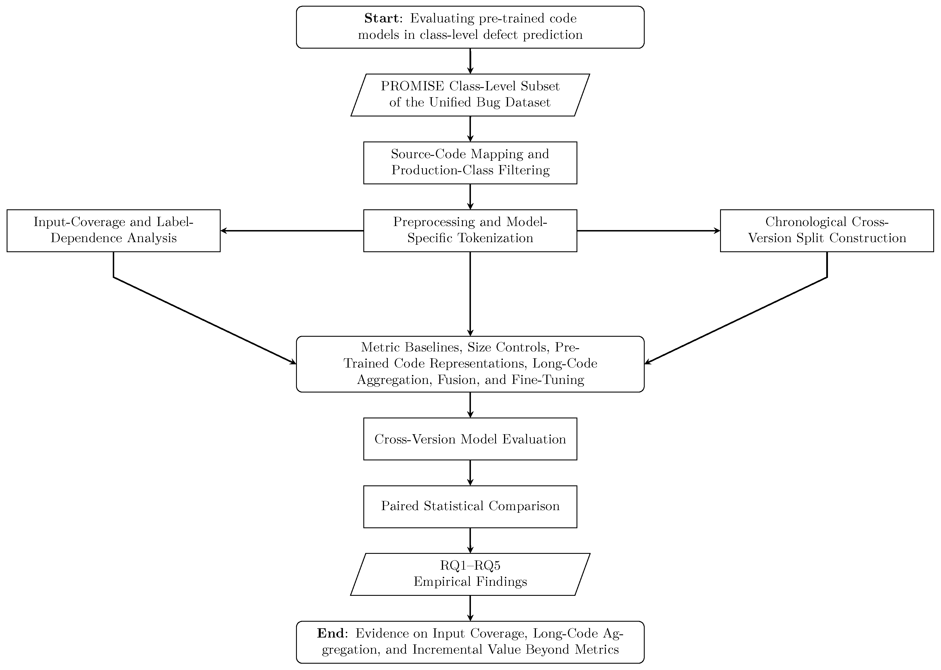
Figure 1 summarizes the empirical workflow followed in this study.
3.2. Dataset and Prediction Units
The study uses the class-level PROMISE subset of the Unified Bug Dataset [
24]. The full Unified Bug Dataset integrates records originating from several source datasets and includes both class-level and file-level prediction units. The present study requires a consistent combination of class-level defect labels, object-oriented software metrics, corresponding version-specific Java source code, and at least three chronologically ordered releases to construct separate training, validation, and test partitions. The class-level PROMISE subset was selected because it provides this combination for multiple projects. Focusing on class-level prediction also aligns the source-code unit with the object-oriented metric baselines and reduces ambiguity when mapping source code to defect labels.
The unit of analysis is a Java class. Each class is treated as one prediction instance and is assigned a binary label: defective or clean. A class is labeled as defective if it is associated with at least one recorded defect in the corresponding dataset version; otherwise, it is labeled as clean. The study focuses on class-level prediction because classes are natural units of design, implementation, testing, and maintenance in object-oriented systems.
The class-level PROMISE projects were screened according to the requirements of the experimental design. A project was eligible for the main predictive analysis when corresponding source-code archives were available, class records could be mapped reliably to production source code, and at least three chronologically ordered releases were available. The project also had to support at least one train–validation–test split satisfying the defective-instance criteria defined in
Section 3.4. Applying these requirements retained Ant, Camel, JEdit, Lucene, Poi, and Synapse. Project selection was therefore determined by data availability and protocol eligibility rather than by the observed predictive performance of the evaluated models.
After source-code mapping and filtering, the cleaned production dataset contains 16,237 class-level instances, including 2522 defective classes and 13,715 clean classes.
Table 2 summarizes the projects used in the study.
3.3. Source-Code Mapping and Filtering
The PROMISE class-level files provide class identifiers, source-code locations, defect labels, and metric values. For each class-level row, we recover the corresponding Java source code using the available metadata fields, including the fully qualified class name, source path, and line-span information. The mapping procedure consists of four steps.
First, the source-code archive for each project version is extracted. Second, all Java files are indexed using normalized relative paths. Third, each class-level dataset row is matched to a Java file using its recorded path and class name, allowing for differences in source-root structure. Fourth, the recorded class span is checked against the extracted source code to verify that the expected class declaration appears in the mapped region.
Rows are excluded from the main dataset if they do not represent ordinary production class-level prediction units. Specifically, we exclude anonymous classes, local classes, synthetic classes, parser-error entries, generated-source classes, test-source classes, and empty-code entries. Test-source classes are identified using path-based patterns such as src/test, src/testcases, /test/, /tests/, and /testcases/. We do not exclude a class only because its name contains the word Test, because production APIs may legitimately use this term. This filtering step is intended to reduce noise and ensure that the prediction instances correspond to production classes.
3.4. Chronological Cross-Version Protocol
The main evaluation protocol is chronological cross-version prediction. For each project, the model is trained on earlier version(s), tuned on the next version, and evaluated on a later version. This protocol reflects the practical setting in which historical project data are used to support quality prediction for future releases.
The rolling procedure generated 12 candidate chronological train–validation–test splits. A candidate split was retained in the main predictive evaluation when the training partition contained at least 20 defective instances, the validation partition contained at least 20 defective instances, and the test partition contained at least 20 defective instances. These values are operational split-support criteria rather than universal minimum requirements for defect-prediction studies.
Eleven candidate splits satisfied these criteria.
Table 3 reports their release assignments. The excluded candidate would have used JEdit 3.2, 4.0, and 4.1 for training, JEdit 4.2 for validation, and JEdit 4.3 for testing. JEdit 4.3 contained 11 defective instances and therefore did not meet the minimum test-partition requirement.
Within each chronological split, median imputation, feature standardization, class-weight calculation, and model fitting are performed using the training partition only. The fitted preprocessing transformations are then applied unchanged to the validation and test partitions. The validation partition is used for model selection, neural-model early stopping, classification-threshold selection, and late-fusion weight selection. Once these choices have been made, the resulting configuration is fixed and applied to the test partition. The test partition is not used during preprocessing estimation, model fitting, model selection, early stopping, threshold tuning, or fusion-weight selection.
3.5. Preprocessing and Tokenization
For each mapped class, the source code corresponding to the verified class span is extracted from the recovered Java file. In the primary preprocessing condition, Java line, block, and Javadoc comments are removed before literal masking and whitespace normalization. The comment scanner preserves comment delimiters occurring inside standard Java string and character literals. Identifiers are retained because class, method, and field names may contain information useful to the pre-trained code models.
Each pre-trained model is evaluated using its corresponding tokenizer. Because the evaluated tokenizers may segment the same Java class differently, input coverage is computed separately for each model. For a model m, let denote the effective code-token budget after reserving positions for the required special tokens. A class is considered overflowing for model m when its number of model-specific code tokens exceeds .
For each class and model tokenizer, we compute the following input-coverage statistics:
the number of model-specific code tokens;
an overflow indicator;
the number of chunks required to encode the class;
the number of tokens discarded under First-window truncation; and
the discarded-token ratio under First-window truncation.
Overflow severity is defined relative to the model-specific token budget :
no overflow: token count ;
mild overflow: ;
moderate overflow: ; and
severe overflow: token count .
This model-specific definition avoids assuming that all tokenizers produce the same token count for the same Java class.
Using the tokenizer-specific coverage framework defined above, we conducted a targeted comment-retention sensitivity analysis to assess whether removing comments disadvantages the learned source-code representations. The sensitivity condition retains all comments available within the verified class span while applying the same literal masking and whitespace normalization as the primary condition.
For each evaluated model, both preprocessing conditions use a 512-position input with an effective code-token budget of , together with the same First-window representation, model checkpoint, tokenizer, frozen encoder, balanced Logistic Regression classifier, random seed 42, and validation-based classification-threshold grid. Comment retention is therefore the only intended preprocessing difference between the two conditions. GraphCodeBERT remains a token-only encoder in this sensitivity analysis.
The coverage component of the sensitivity analysis uses all 16,237 cleaned class-version instances. The predictive component uses the 15,223 unique instances appearing in the 11 retained chronological splits. For each split, the training releases are used to fit the classifier, validation MCC is used to select the classification threshold, and the fitted classifier and selected threshold are then applied unchanged to the held-out test release.
3.6. Pre-Trained Code Models
The main experiments evaluate three pre-trained code models: CodeBERT, GraphCodeBERT, and CodeT5. These models are selected because they represent widely used families of pre-trained code encoders and allow the study to move beyond a CodeBERT-only analysis.
CodeBERT is included as a reference model because it is one of the most widely used pre-trained models for programming language and natural language representations [
11]. GraphCodeBERT is included because it extends pre-trained code representation learning by incorporating data-flow information during pre-training [
12]. CodeT5 is included because it is an identifier-aware encoder–decoder model designed for code understanding and generation tasks [
13].
Table 4 summarizes the pre-trained models used in the study.
The main frozen-representation experiments use each model as an encoder and train a downstream defect classifier separately for each chronological split. The encoder parameters are not updated in the frozen setting. For encoder-only models, the final hidden representation of the classification token is used as the sequence representation. For CodeT5, the class representation is obtained by mean pooling over the final encoder hidden states corresponding to non-padding tokens. The exact representation-extraction strategy is fixed before model evaluation and is applied consistently across all splits.
3.7. GraphCodeBERT Data-Flow Sensitivity Protocol
The main GraphCodeBERT experiments use the public microsoft/graphcodebert-base checkpoint with token-sequence input only. To determine whether this choice underestimates GraphCodeBERT, we conducted a targeted sensitivity analysis using the frozen First-window representation and the same 11 chronological train–validation–test splits.
Three conditions were evaluated. The first was the original token-only condition with a maximum of 510 code subtokens. The second was a budget-matched token-only condition with a maximum of 382 code subtokens. The third supplied a maximum of 382 code subtokens together with up to 128 Java data-flow graph (DFG) nodes. The budget-matched token-only condition controls for the reduction in code-token capacity caused by reserving input positions for data-flow nodes.
Java source code was parsed using Tree-sitter 0.25.2 and tree-sitter-java 0.23.5. Data flow was extracted from the verified class source span. The explicit data-flow condition included code tokens, DFG nodes, DFG-to-code mappings, DFG-to-DFG edges, GraphCodeBERT position indices, and a graph-guided two-dimensional attention mask supplied to the model forward pass. Instances producing an empty DFG were retained using an empty data-flow component rather than being removed.
All three conditions used identical class-version instances and chronological partitions. The GraphCodeBERT encoder remained frozen, and the same downstream Logistic Regression classifier, class-weighting procedure, random seed, and validation-based threshold-selection rule were used. The primary planned comparisons were: (i) the original 510-token condition versus the 382-token condition, which measures the effect of reducing the token budget; and (ii) the 382-token condition versus the explicit data-flow condition, which isolates the incremental effect of data-flow input under a matched code-token budget. Holm correction was applied across these two comparisons. The direct comparison between the original token-only and data-flow conditions was treated as contextual because it changes both the code-token budget and the downstream input structure.
3.8. Input-Representation Strategies
To evaluate the effect of input coverage, each pre-trained model is tested using a controlled progression of truncation-based and long-code-aware representations. First-window represents the common default of retaining the beginning of an overlength input, while Last-window and Head-tail test whether retaining alternative source-code regions changes prediction under the same token budget. Chunk-mean and Chunk-max use the same non-overlapping chunks and frozen encoder but add no trainable aggregation parameters, thereby isolating the effect of increased source-code coverage. Chunk attention uses the same chunk embeddings but learns a scalar weight for each chunk, allowing us to test whether trainable aggregation improves over fixed pooling.
Other long-code strategies are available, including overlapping windows, method-level or hierarchical aggregation, learned chunk selection, sparse-attention models, and dedicated long-context encoders. These alternatives change the segmentation scheme, encoder architecture, or model capacity and are therefore outside the scope of the present controlled comparison. The selected strategies are intended as reproducible baselines rather than an exhaustive evaluation of all long-code architectures.
3.8.1. Truncation Baselines
The truncation baselines represent common fixed-window strategies used when a class exceeds the model input budget. For a model with effective token budget , we evaluate the following views:
First-window. The first code tokens are retained and the rest of the class is discarded.
Last-window. The last code tokens are retained and the earlier part of the class is discarded.
Head-tail. The first and last code tokens are retained and concatenated.
The First-window strategy reflects the common default behavior of truncating inputs from the end. The Last-window and Head-tail strategies are included to test whether defect-relevant information is more likely to appear near the end of the class or distributed between the beginning and end.
3.8.2. Simple Chunk Aggregation
The simple long-code baselines split each class into non-overlapping chunks of at most code tokens. Each chunk is encoded independently using the same frozen pre-trained model. The resulting chunk embeddings are then aggregated into a single class-level vector.
We evaluate two simple aggregation strategies:
These strategies test whether increasing input coverage alone is sufficient to improve defect prediction. They are intentionally simple and serve as reproducible long-code-aware baselines rather than as new model architectures. To limit the computational and memory requirements of extremely long classes, the number of retained chunks is capped at . This was a fixed experimental setting rather than a searched hyperparameter. Classes requiring more than 32 chunks are truncated at this cap.
3.8.3. Trainable Chunk Attention
Because fixed mean and maximum pooling cannot learn whether some chunks should contribute more strongly than others, we also evaluate a lightweight trainable chunk-attention model. For a class with
retained chunks, indexed by
, the unnormalized attention score assigned to chunk
i is
where
is the frozen
d-dimensional representation of chunk
i,
is a trainable attention-weight vector, and
is a trainable bias. Padded chunk positions are masked before normalization.
Let
denote the set of valid, non-padding chunks. The normalized weight assigned to a valid chunk is
where
j is the summation index over the set
of valid, non-padding chunks. For padded positions,
. Thus,
and
. The class-level representation is
The vector is passed to a trainable linear classifier with weight vector and bias , followed by a sigmoid transformation to obtain the defective-class probability. The trainable parameters are therefore , , , and ; the pre-trained encoder remains frozen.
The attention layer and final classifier are fitted using only the training partition of each chronological split. The validation partition is used for early stopping and classification-threshold selection. Class imbalance is handled using the weighted binary cross-entropy procedure described in
Section 3.12.
To examine whether the model learned differentiated chunk weighting, we conducted a diagnostic-only rerun of the existing chunk-attention configurations using the same cached chunk embeddings, chronological splits, random seed, training settings, early-stopping rule, and threshold-selection procedure. For each validation and test instance, we recorded the learned attention weights, normalized attention entropy, effective number of attended chunks, highest-weight chunk position, and cosine similarity between the attention-pooled representation and the corresponding Chunk-mean representation. Normalized entropy was calculated only for instances containing at least two valid chunks because a one-chunk instance necessarily receives an attention weight of one.
3.9. Traditional Metric Baselines and Size Controls
Traditional software metrics are used as strong baselines and as controls for interpreting the value of learned code representations. The metric set is taken from the Unified Bug Dataset and includes size, complexity, coupling, cohesion, inheritance, and related object-oriented measures.
We evaluate the following metric-based models:
Logistic Regression using the complete 80-predictor metric set;
Random Forest using the complete 80-predictor metric set;
XGBoost using the complete 80-predictor metric set;
Logistic Regression using only lines of code;
Logistic Regression using only model-specific token count.
For the three full-metric baselines, the same 80 software-metric predictors were used across all 11 chronological splits. The predictor set comprises 60 metrics from the common OpenStaticAnalyzer suite added during construction of the Unified Bug Dataset and 20 metrics retained from the original PROMISE dataset. The Unified Bug Dataset retains the original metrics alongside the common OpenStaticAnalyzer suite because similarly named metrics calculated by different tools may differ in their definitions or calculation procedures [
24]. The exact predictor names are listed in
Appendix A. No feature-selection or dimensionality-reduction procedure was applied.
The LOC-only and token-count-only models serve as size controls. They test whether predictive performance is mainly driven by class size rather than by richer structural or semantic information.
For metric-based models, missing values are imputed using medians computed from the training partition of each split. Standardization is fitted on the training partition and applied to validation and test partitions for Logistic Regression. Tree-based models use imputed but unstandardized features.
The class-imbalance procedures applied across all model families are described separately in
Section 3.12.
3.10. Incremental-Value and Fusion Analysis
A central goal of the study is to determine whether pre-trained code representations add predictive value beyond traditional software metrics. For this reason, the primary comparison is not only between code models and metric models, but also between metric-only models and metric-plus-code models.
We evaluate two forms of fusion.
3.10.1. Early Fusion
Early fusion concatenates a learned code representation with the software-metric feature vector. The combined vector is then used to train a downstream classifier. For frozen pre-trained representations, early fusion is evaluated using Logistic Regression and, where appropriate, a tree-based classifier.
The complete early-fusion condition uses the 80-predictor metric set described in
Section 3.9. An auxiliary early-fusion condition excludes eight LOC-family measures from the complete metric set, leaving 72 predictors. We refer to this condition as the LOC-excluded metric set.
The primary early-fusion comparison is:
This comparison tests whether the learned representation contains defect-relevant information that is not already captured by traditional metrics.
3.10.2. Late Fusion
Late fusion combines predicted probabilities from a metric-based model and a pre-trained-code model. Let
denote the probability produced by the metric model and
denote the probability produced by the code-representation model. The fused probability is:
The parameter controls the relative contribution of the two models: corresponds to the metric-only prediction, whereas corresponds to the code-only prediction. For each chronological split, the metric-based classifier with the highest validation MCC was first selected from Logistic Regression, Random Forest, and XGBoost. The selected metric model was then paired separately with each frozen pre-trained encoder and input-representation configuration.
For each resulting combination, and the classification threshold were selected jointly using the validation partition. The fusion-weight grid was , and the threshold grid was . The pair that maximized validation MCC was retained. Ties were resolved deterministically by retaining the first pair encountered in ascending grid order. The selected fusion weight and threshold were then fixed and applied unchanged to the corresponding test partition. Test-set performance was not used in metric-model selection, fusion-weight selection, or threshold selection. The selected split-specific fusion weights are provided in the replication package.
Late fusion tests whether independently trained metric and code models provide complementary decision-level information.
3.11. Fine-Tuning Robustness Check
The main experiments use frozen encoders because this setting isolates the transferability of pre-trained code representations and makes the comparison between truncation, aggregation, and metric baselines easier to interpret. However, conclusions based only on frozen representations may underestimate the value of pre-trained code models. Therefore, we include supervised fine-tuning as a targeted robustness check.
To avoid an unmanageable number of configurations, fine-tuning is applied only to the First-window input strategy for each pre-trained model. The purpose is not to optimize every possible long-code configuration, but to test whether task-specific adaptation changes the main conclusion about the value of pre-trained code models beyond metrics.
For each chronological split, the encoder and classification head are fine-tuned using only the training version(s). Each encoder–split condition is repeated using three predetermined random seeds, , yielding 99 fine-tuning runs. The seed set was fixed before inspecting the multi-seed predictive results and was not selected according to validation or test performance.
The fine-tuning configuration is fixed across all seeds: a 512-position First-window input, AdamW optimization with learning rate
and weight decay 0.01, batch size 8, a linear learning-rate schedule with no warm-up, a maximum of five epochs, and early-stopping patience of two. Class imbalance is handled using the weighted cross-entropy procedure defined in
Section 3.12. No separate hyperparameter search is conducted for individual seeds.
The fine-tuning experiments use Python 3.10.20, NumPy 2.2.6, and PyTorch 2.8.0 with CUDA 12.8. For every run, the corresponding seed is applied to the Python standard-library random generator, the NumPy random-number generator, and the PyTorch CPU and CUDA random-number generators. The seed also controls model-head initialization, dropout, and shuffled training-batch order. DataLoader workers are not used (num_workers=0). The best epoch is selected using validation MCC. The classification threshold is then selected from using the selected checkpoint’s validation probabilities, with the first threshold in ascending order retained when MCC ties. The selected checkpoint and threshold are applied unchanged to the held-out test version. PyTorch deterministic algorithms are not enabled, so some residual GPU-level nondeterminism may remain.
The fine-tuning robustness check supports the following interpretation. If fine-tuned models substantially outperform frozen representations and add value beyond metric baselines, then frozen representations underestimate the potential of pre-trained code models. If fine-tuned models still fail to improve over strong metric baselines, then the evidence suggests that traditional software metrics remain difficult baselines to beat under chronological class-level prediction.
3.12. Class-Imbalance Treatment
The cleaned dataset is imbalanced, containing 2522 defective and 13,715 clean class-version instances. Because defect prevalence varies across project releases and chronological splits, all class-imbalance parameters are calculated separately from the training partition of each split. Let and denote the numbers of clean and defective training instances, respectively. The model-specific procedures are as follows:
Logistic Regression-based classifiers and Random Forest use class_weight=balanced;
XGBoost uses scale_pos_weight;
trainable chunk attention uses weighted binary cross-entropy with pos_weight = ; and
supervised fine-tuning uses weighted cross-entropy with class weights .
No oversampling, undersampling, or synthetic resampling is used. The validation and test partitions retain their observed class distributions and are not altered using information from the training partition.
Cost-sensitive weighting was selected because it preserves the observed set of historical training instances, avoids introducing duplicated or synthetic class records, and provides a consistent imbalance treatment across the traditional classifiers, frozen-representation classifiers, trainable chunk-attention model, and fine-tuned encoders. This choice is not claimed to be universally optimal. Alternative oversampling, undersampling, or hybrid procedures may produce different defect-detection and false-positive trade-offs, and their systematic comparison remains outside the representation-focused scope of this study.
To make the resulting operational trade-offs visible, performance is evaluated using MCC together with precision, recall, F1-score, PR-AUC, G-mean, and balanced accuracy, as described in
Section 3.14. Classification thresholds are selected using only the validation partition and are applied unchanged to the corresponding held-out test release.
3.13. Label-Dependence and Size-Controlled Analysis
RQ2 examines whether input overflow is associated with defect labels. We first compare overflow rates between defective and clean classes using contingency tables, odds ratios, chi-square tests, and Fisher’s exact tests. We then examine the defective-class ratio across overflow severity groups.
Because defective classes may also be larger or more complex than clean classes, we perform a size-controlled analysis. Specifically, we fit logistic regression models of the following form:
A second model replaces the binary overflow indicator with overflow severity. The goal of this analysis is not to claim that overflow causes defects. Rather, the goal is to determine whether input overflow is associated with the defect label after accounting for basic size and project-version effects. If overflow remains associated with defect labels, then truncation should be treated as a representation-validity concern because incomplete input coverage is not randomly distributed across defective and clean classes.
3.14. Evaluation Metrics
The primary evaluation metric is Matthews Correlation Coefficient (MCC). MCC is used because class-level defect prediction is typically imbalanced and MCC accounts for all four entries of the confusion matrix. We also report precision, recall, F1-score, area under the ROC curve (AUC-ROC), area under the precision–recall curve (PR-AUC), G-mean, and balanced accuracy.
Because class-imbalance treatment and threshold selection can alter the trade-off between detecting defective classes and generating false positives, we interpret recall and precision jointly with MCC, F1, PR-AUC, G-mean, and balanced accuracy rather than relying on accuracy alone.
For models that produce probabilities, the classification threshold is selected separately within each chronological split using the validation partition. Candidate thresholds are evaluated over
, and the threshold that maximizes validation MCC is retained. When multiple thresholds produce the same MCC, the first threshold encountered in ascending order is retained. The selected threshold is then applied unchanged to the corresponding test partition. For late fusion, the threshold is selected jointly with the fusion weight, as described in
Section 3.10.2.
The primary reported performance values are computed on the test versions of the 11 chronological splits. We report mean and median performance across splits, together with per-split values in the replication package. Reporting per-split values is important because average performance can hide substantial project-version variability.
3.15. Statistical Analysis
Model comparisons are performed using paired split-level results. For each comparison, both models are evaluated on the same chronological split, producing paired performance values. The primary statistical analysis uses MCC because it is the main evaluation metric.
We use the Wilcoxon signed-rank test for paired comparisons because the number of splits is small and normality cannot be assumed. Since multiple comparisons are performed, Holm correction is applied to control the family-wise error rate. In addition to corrected p-values, we report Cliff’s delta as a non-parametric effect-size measure. Positive Cliff’s delta values indicate that the candidate model tends to outperform the baseline model, whereas negative values indicate the opposite.
Holm correction is applied separately within each coherent family of comparisons associated with a research question or targeted sensitivity analysis, rather than across every statistical test reported in the study. These families include the long-code representation comparisons for RQ3, the incremental-value and fusion comparisons for RQ4, the three encoder-specific fine-tuning comparisons for RQ5, and the comparisons within each targeted sensitivity analysis. Comparisons within a family address the same inferential objective and are interpreted together.
This family-level approach controls the family-wise error rate for each related set of claims while avoiding a single study-wide correction that would combine conceptually distinct hypotheses, baselines, and experimental questions. Accordingly, each Holm-adjusted p-value should be interpreted relative to its corresponding comparison family and should not be interpreted as controlling the probability of any false-positive result across all statistical analyses reported in the manuscript.
For RQ5, individual seed runs are not treated as independent observations. Each test metric is first averaged arithmetically across the three seeds within each chronological split. The resulting 11 split-level means are then compared with the corresponding frozen First-window values. Within-split sample standard deviations and ranges are reported descriptively to characterize stochastic variation; seed probabilities are not ensembled.
The main statistical comparisons are:
long-code aggregation versus truncation baselines;
trainable chunk attention versus fixed chunk pooling;
pre-trained-code-only models versus metric-only models;
metric-plus-code fusion models versus metric-only models;
fine-tuned models versus corresponding frozen models.
The most important comparison for practical interpretation is whether adding a pre-trained code representation to a strong metric baseline improves performance consistently across chronological splits. This comparison directly tests the incremental value of learned code representations beyond established software-quality indicators.
Here, and denote the numbers of clean and defective instances, respectively, in the corresponding training partition, and p denotes the number of predictor features.
3.16. Computational-Cost Profiling
To characterize the implementation trade-offs among the evaluated method families, we profiled the existing implementations on the Lucene-1 chronological split, comprising Lucene 2.0 for training, Lucene 2.2 for validation, and Lucene 2.4 for testing. The split contains 496 training, 891 validation, and 896 test class-version instances, for a total of 2283 instances. It was selected before profiling because its total instance count equals the median across the 11 retained chronological splits and its model-specific token and chunk workloads fall within the interquartile range.
Wall-clock time was measured using time.perf_counter. For GPU-based stages, the GPU was synchronized immediately before and after each timed region, and peak allocated GPU memory was measured using torch.cuda.max_memory_allocated. Model and tokenizer loading, local checkpoint loading, downloads, environment setup, and queue time were excluded.
Except for supervised fine-tuning, each encoder-specific stage was evaluated using one warm-up followed by three measured repetitions, and the median was reported. Fine-tuning was measured once for each of CodeBERT, GraphCodeBERT, and CodeT5 because it required end-to-end encoder optimization; the reported family-level value is the median across the three encoder-specific measurements. For other rows representing all three encoders, the reported value is the median of the encoder-specific medians. Complete per-encoder and per-repetition measurements are provided in the replication package.
For frozen models, representation extraction was measured separately from downstream classifier fitting because the resulting embeddings can be cached and reused. The reported frozen-extraction times cover the training, validation, and test partitions, whereas the reported milliseconds per class are calculated from a separate test-only extraction measurement. Chunk encoding was measured separately from fixed pooling and trainable chunk attention. For early and late fusion, the costs of generating the underlying representations or probabilities were not counted again. The metric-model measurements assume that the software metrics are already available and therefore do not include the upstream cost of extracting static metrics from source code.
The measurements were obtained using an NVIDIA GeForce RTX 5070 Ti Laptop GPU with 12,227 MiB of GPU memory, an Intel Core Ultra 9 275HX CPU, and 31.4 GiB of system memory. They are intended to support relative comparison under the reported implementation and hardware rather than to provide hardware-independent runtime estimates.
3.17. Reproducibility Measures
The main fixed-configuration experiments use a random seed of 42 where applicable. This seed controls Python, NumPy, PyTorch CPU, PyTorch CUDA, and the random-state parameters of the traditional classifiers. Supervised fine-tuning is repeated using three predetermined seeds, . For fine-tuning, each seed is applied independently before model construction and DataLoader initialization. Seed-specific test metrics are averaged within each chronological split before paired statistical analysis. PyTorch deterministic algorithms are not enforced; consequently, some residual GPU-level nondeterminism may remain.
The fixed model configurations, random seeds, and validation-based selection procedures are summarized in
Table 5. Classification thresholds are selected on the validation partition by maximizing MCC. For chunk attention and supervised fine-tuning, validation MCC is also used for best-epoch selection with patience-based early stopping.
The experiments were conducted with Python 3.10.20, NumPy 2.2.6, scikit-learn 1.7.2, XGBoost 3.2.0, PyTorch 2.8.0 with CUDA 12.8, and Transformers 4.26.0.
4. Results
This section reports the empirical findings for RQ1–RQ5. All predictive results are computed on the held-out test versions of the 11 chronological cross-version splits. The validation versions are used only for model selection, threshold tuning, fine-tuning early stopping, and late-fusion weight selection. MCC is the primary metric. F1, PR-AUC, AUC-ROC, recall, and balanced accuracy are reported as secondary metrics.
4.1. RQ1: Input Coverage Across Pre-Trained Code Models
RQ1 examines input coverage under the main token-only representation protocol. Although all three checkpoints in this main analysis use a 512-position input window, input coverage is not identical across models because token counts are tokenizer-specific. After reserving positions for the required special tokens, we use an effective code-token budget of 510 tokens for the window-based and chunk-based representations. Overflow is therefore computed separately for each model–tokenizer pair.
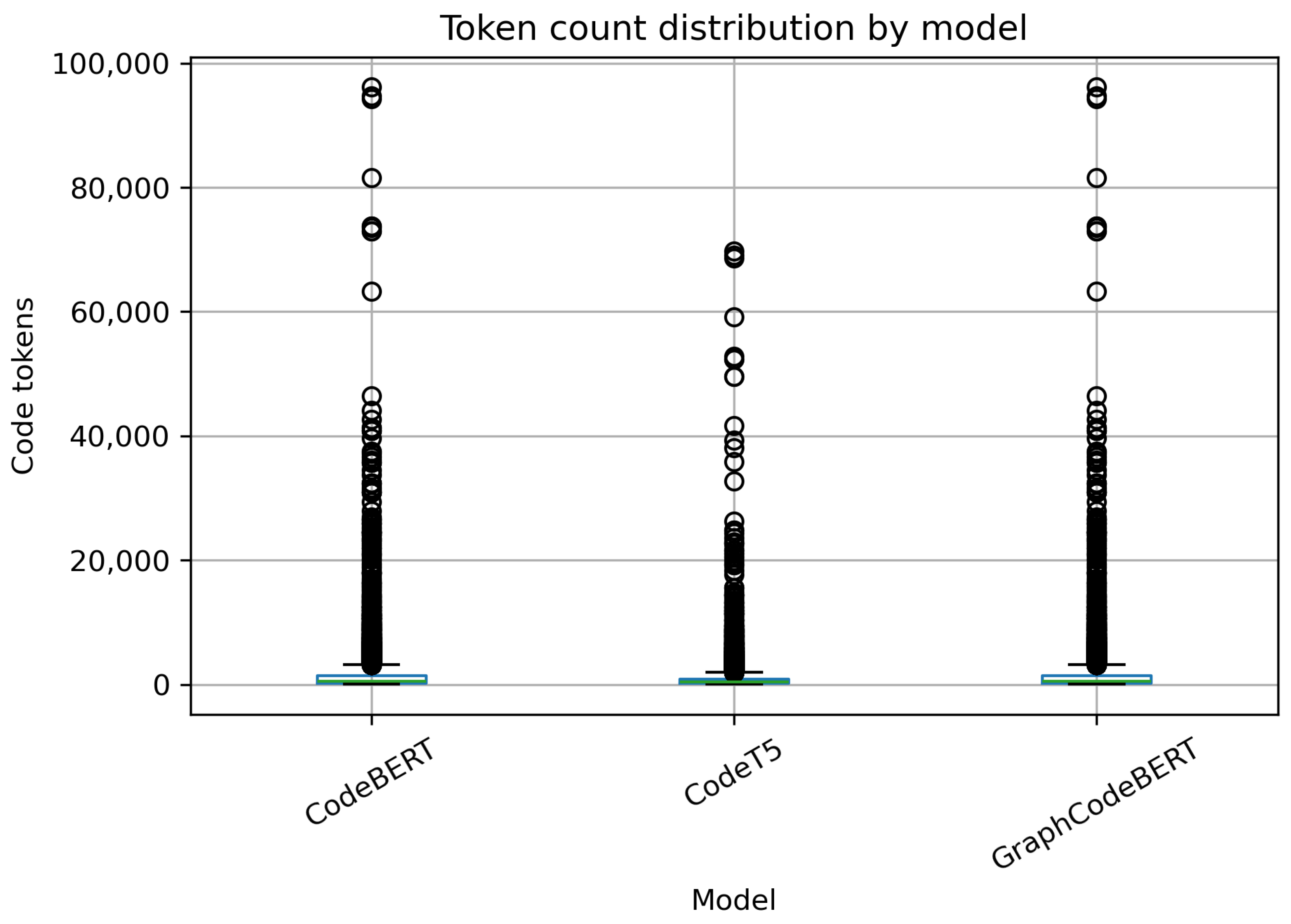
Table 6 and
Figure 2 show that input overflow is common for all evaluated models. CodeBERT and GraphCodeBERT overflow for 8238 of 16,237 classes, corresponding to an overflow rate of 50.7%. CodeT5 has a lower overflow rate, with 6327 overflowing classes, corresponding to 39.0% of the dataset.
The lower overflow rate for CodeT5 does not mean that the underlying Java classes are shorter. Rather, it reflects tokenizer-specific segmentation: the same Java class can produce fewer CodeT5 tokens than CodeBERT or GraphCodeBERT tokens. Accordingly, overflow rates should be interpreted as model-tokenizer-specific input coverage statistics rather than model-independent source-code length measures.
The identical input-coverage statistics for CodeBERT and GraphCodeBERT indicate that, in this experiment, both models use the same tokenization profile for the token-only input setting. Their downstream differences therefore reflect differences in representation learning and model behavior rather than differences in token-count coverage.
The chunk-distribution results further confirm that many classes require multiple input windows. CodeBERT and GraphCodeBERT require a mean of 3.31 chunks per class, with a median of 2 chunks, a 90th percentile of 7 chunks, a 95th percentile of 11 chunks, and a 99th percentile of 27 chunks. CodeT5 requires fewer chunks on average, with a mean of 2.29 chunks and a median of 1 chunk, but its 95th and 99th percentiles are still 7 and 16 chunks.
Answer to RQ1. Class-level input overflow is common across the evaluated pre-trained code models. The severity differs by tokenizer, with CodeT5 producing fewer overflowing inputs than CodeBERT and GraphCodeBERT, but even CodeT5 overflows for 39.0% of classes. These results show that input coverage is a non-trivial issue for class-level defect prediction with fixed-length pre-trained code models and should be reported at the model-tokenizer level.
4.2. RQ2: Label-Dependent Overflow and Size-Controlled Analysis
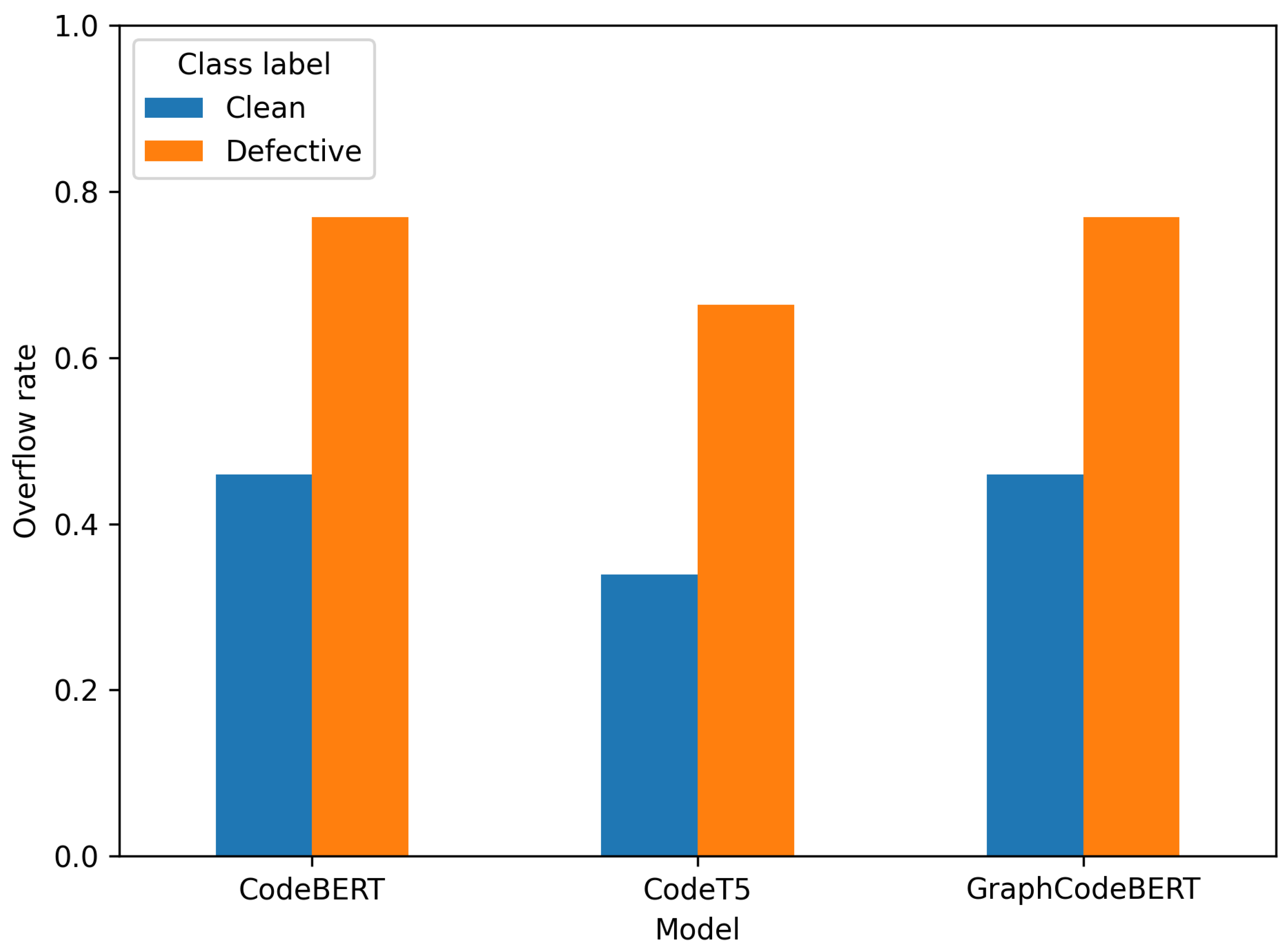
RQ2 examines whether input overflow is associated with defect labels. The label-based overflow results are shown in
Table 7 and
Figure 3. For all evaluated models, defective classes overflow substantially more often than clean classes.
For CodeBERT and GraphCodeBERT, 76.9% of defective classes overflow, compared with 45.9% of clean classes. The corresponding odds ratio is 3.93. For CodeT5, 66.4% of defective classes overflow, compared with 33.9% of clean classes. The corresponding odds ratio is 3.84. The Fisher exact tests in
Table 8 indicate very small
p-values in the uncontrolled association analysis.
The token-count differences by label are also large. For CodeBERT and GraphCodeBERT, defective classes have a median length of 1343 tokens, whereas clean classes have a median length of 435 tokens. For CodeT5, defective classes have a median length of 852.5 tokens, whereas clean classes have a median length of 291 tokens.
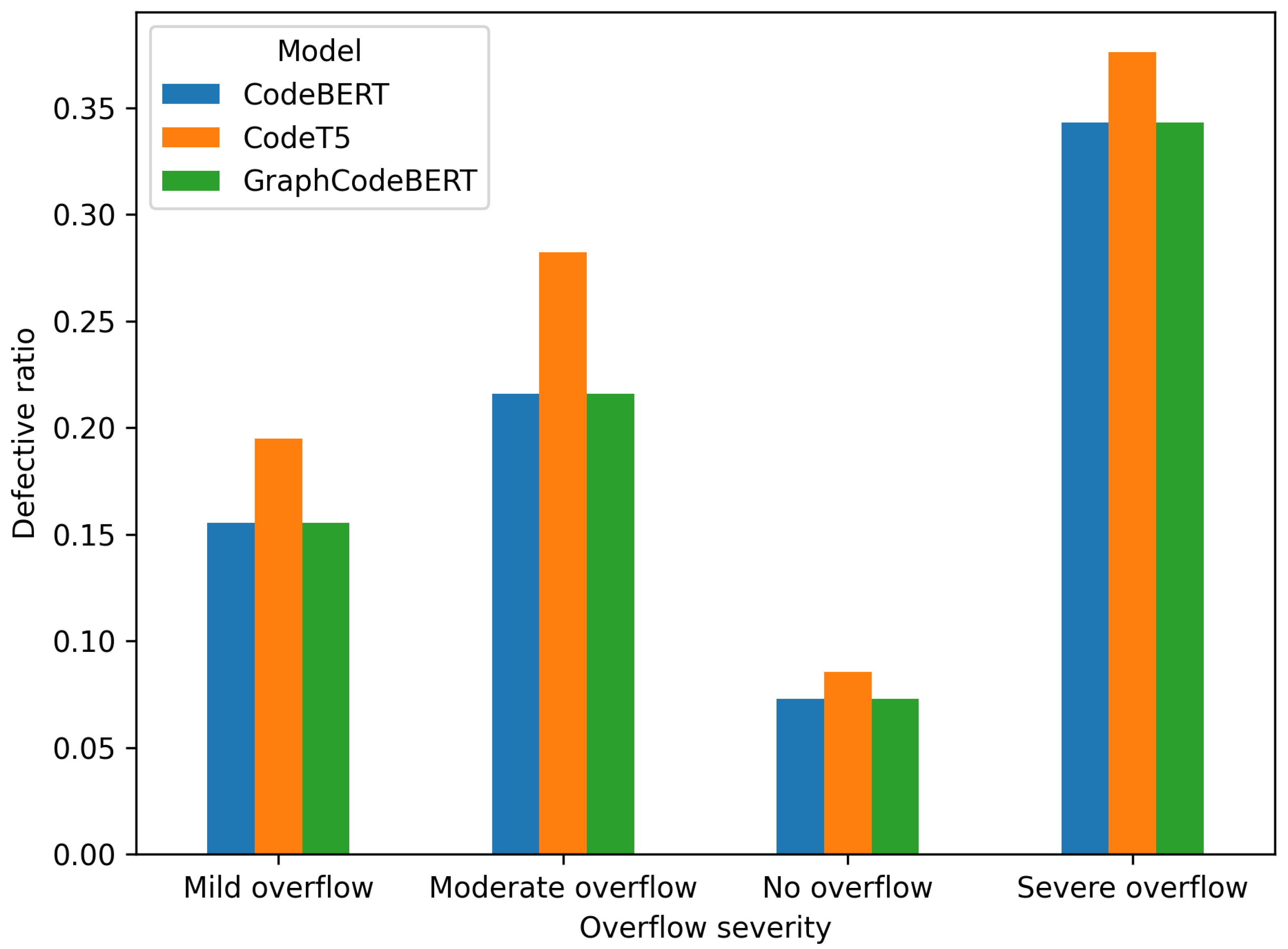
Figure 4 shows the relationship between overflow severity and the defective-class ratio. For CodeBERT and GraphCodeBERT, the defective ratio increases from 7.3% in the no-overflow group to 15.5% in the mild-overflow group, 21.6% in the moderate-overflow group, and 34.3% in the severe-overflow group. For CodeT5, the corresponding ratios are 8.6%, 19.5%, 28.2%, and 37.6%.
Table 9 reports selected coefficients from the controlled overflow models. Model A uses a binary overflow indicator, while Model B uses overflow severity. The controlled models include log LOC, log token count, project terms, and version terms. The results show that the overflow coefficients remain positive after accounting for size-related and project-version factors. For the binary overflow indicator, the odds ratios are 1.325 for CodeBERT and GraphCodeBERT and 1.333 for CodeT5. For severe overflow, the odds ratios are 2.266 for CodeBERT and GraphCodeBERT and 1.644 for CodeT5. All reported confidence intervals are above 1.0 and all Wald
p-values are below 0.001, indicating that the controlled associations remain statistically supported. Although these effects are smaller than the uncontrolled odds ratios reported in
Table 8, they show that overflow remains positively associated with defect labels after controlling for size-related and project-version factors.
Answer to RQ2. The uncontrolled results show a strong association between input overflow and defect labels for all evaluated models. Defective classes are much more likely to overflow than clean classes, and the defective-class ratio increases with overflow severity. The controlled logistic models show that overflow remains positively associated with defect labels after controlling for size-related and project-version factors. The effect is smaller than the uncontrolled association but remains statistically supported: the overflow-indicator odds ratios are 1.325 for CodeBERT and GraphCodeBERT and 1.333 for CodeT5, while the severe-overflow odds ratios are 2.266 for CodeBERT and GraphCodeBERT and 1.644 for CodeT5. Therefore, input overflow is not only common but also label-dependent, which supports treating input coverage as a representation-validity concern in class-level defect prediction with fixed-length pre-trained code models.
4.3. RQ3: Long-Code Aggregation Versus Truncation
RQ3 evaluates whether long-code-aware representation strategies improve defect prediction over truncation-based representations.
Table 10 reports the mean MCC of the code-only representation strategies across the 11 chronological splits.
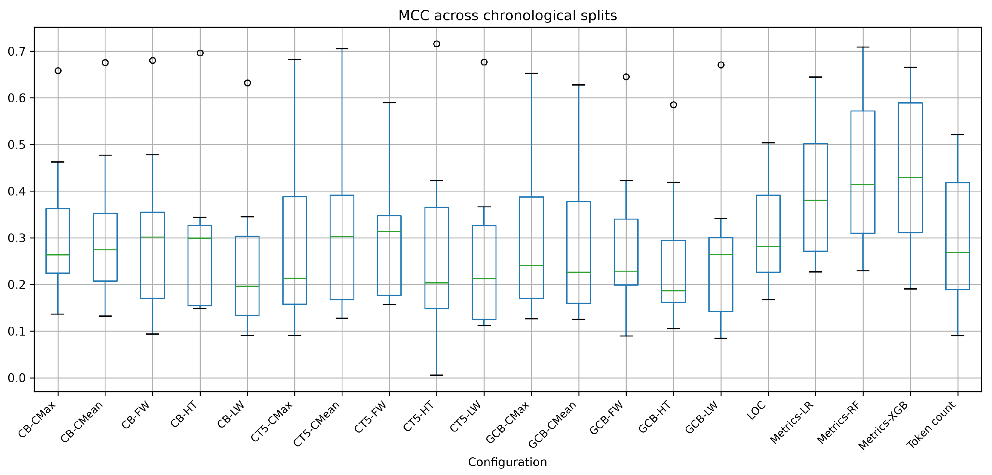
Figure 5 shows the split-level MCC distributions.
For CodeBERT-only models, chunk-max obtains the highest mean MCC of 0.315, followed by chunk-mean with 0.307 and first-window truncation with 0.298. Head-tail and last-window truncation obtain lower mean MCC values of 0.286 and 0.240, respectively. The trainable chunk-attention model obtains a lower mean MCC of 0.129.
For CodeT5-only models, chunk-mean obtains the highest mean MCC of 0.309, followed by chunk-attention with 0.295 and first-window truncation with 0.291. For GraphCodeBERT-only models, chunk-max obtains the highest mean MCC of 0.292, followed by chunk-mean with 0.286 and first-window truncation with 0.283.
Table 11 reports selected paired MCC comparisons between long-code strategies and first-window truncation. All Holm-corrected
p-values in these selected comparisons are 1.000.
The fixed chunk-pooling improvements are small. CodeBERT chunk-max improves over first-window by 0.017 MCC, with six wins and five losses across the 11 splits. CodeT5 chunk-mean improves over first-window by 0.018 MCC, with seven wins and four losses. GraphCodeBERT chunk-max improves over first-window by 0.009 MCC, with five wins and six losses. None of these improvements survives Holm correction.
The trainable chunk-attention results are mixed. CodeT5 chunk-attention is only 0.004 MCC above first-window, while CodeBERT and GraphCodeBERT chunk-attention are below first-window by 0.169 and 0.038 MCC, respectively. For CodeBERT, chunk-attention is also lower than chunk-max by 0.186 MCC; this comparison has an uncorrected Wilcoxon , but the Holm-corrected value is 0.498. Thus, no corrected statistical claim is made for chunk-attention.
To examine the behavior of the learned attention mechanism, we analyzed the attention weights produced for the validation and test instances. For instances containing at least two chunks, median normalized attention entropy ranged from 0.996 to 0.999 across the encoder and partition summaries, where a value of one denotes uniform weighting. The median cosine similarity between the attention-pooled and Chunk-mean representations was at least across all encoder and partition summaries, indicating that the two representations were nearly identical.
The model therefore did not generally collapse onto a single chunk. Instead, it assigned mostly diffuse weights and produced class representations that were nearly indistinguishable from mean pooling. This behavior helps explain why the learned attention mechanism did not provide a robust predictive improvement.
Answer to RQ3. Long-code-aware strategies provide only limited and inconsistent improvements over truncation. Fixed chunk pooling produces small positive mean MCC changes for some model–strategy combinations, but none of the improvements survives Holm correction. The trainable chunk-attention model does not provide a robust improvement in the evaluated setting.
4.4. RQ4: Incremental Value Beyond Traditional Metrics
RQ4 evaluates whether pre-trained code representations add predictive value beyond traditional software metrics and size controls.
Table 12 summarizes selected mean test performance values across the 11 chronological splits. The table includes standalone metric baselines, size-only controls, the strongest code-only configurations, early fusion, late fusion, and fine-tuned models.
The metric-only baselines remain strong. Random Forest trained on traditional software metrics obtains the best standalone mean MCC of 0.451. XGBoost obtains an MCC of 0.439, and Logistic Regression obtains an MCC of 0.397. The validation-selected best-metric baseline, which is selected separately within each split using validation data, obtains a mean MCC of 0.443.
The best code-only model is CodeBERT chunk-max with mean MCC of 0.315. This is close to the LOC-only baseline, which obtains MCC of 0.313, and slightly above the token-count-only baseline, which obtains MCC of 0.302. However, it remains below the metric LR, XGBoost, and RF baselines. The best CodeT5-only and GraphCodeBERT-only configurations obtain MCC values of 0.309 and 0.292, respectively.
Table 13 reports selected incremental-value comparisons. The code-only comparisons against metric RF are negative for all three selected code-only models. CodeBERT chunk-max is lower than metric RF by 0.135 MCC, with 0 wins and 11 losses across the chronological splits. CodeT5 chunk-mean is lower by 0.141 MCC, with 2 wins and 9 losses. GraphCodeBERT chunk-max is lower by 0.159 MCC, with 0 wins and 11 losses. These comparisons do not reach significance after Holm correction, although the effect directions are consistently negative.
Early fusion does not improve over the validation-selected best metric baseline. The strongest early-fusion row in
Table 12 is CodeBERT chunk-max with the complete metric set, which obtains a mean MCC of 0.372. The corresponding condition using the LOC-excluded metric set obtains a mean MCC of 0.368. In the paired incremental-value comparison, CodeBERT chunk-max with the complete metric set has ΔMCC of −0.071 relative to the validation-selected best metric baseline, with 1 win and 10 losses.
Late fusion performs better than early fusion, but the improvement remains small and does not survive Holm correction. The strongest late-fusion configuration averaged over all 11 splits is GraphCodeBERT chunk-mean late fusion, with a mean MCC of 0.459. Relative to the validation-selected best metric baseline, this corresponds to ΔMCC of 0.016, with six wins, four losses, one tie, Holm , and Cliff’s . CodeBERT chunk-max late fusion has ΔMCC of 0.010, while CodeT5 chunk-max late fusion has ΔMCC of 0.001. These values indicate small improvements in some splits, but not Holm-adjusted statistical evidence of robust incremental value.
The selected late-fusion weights also indicate substantial reliance on the metric component. Across the 165 split- and configuration-specific selections, the mean metric weight is 0.811. Thus, on average, the validation-selected late-fusion models place considerably greater weight on the metric-based probability than on the code-based probability.
Answer to RQ4. The results do not provide corrected statistical evidence that pre-trained code representations add substantial incremental value beyond traditional software metrics. Metric-based Random Forest remains the strongest standalone baseline by mean MCC. Code-only models are close to size-only controls but below the strongest metric baselines. Early fusion does not improve over metrics, and late fusion produces only small, non-significant improvements after Holm correction.
4.5. RQ5: Fine-Tuning Robustness Check
RQ5 examines whether supervised fine-tuning changes the conclusions obtained from frozen representations. The analysis is limited to First-window inputs for CodeBERT, GraphCodeBERT, and CodeT5. Each encoder–split condition is evaluated using three predetermined seeds, and the seed-specific test metrics are averaged within each chronological split before the split-level comparisons.
As shown in
Table 12, fine-tuning increases mean MCC relative to the corresponding frozen First-window representation for all three encoders. CodeBERT improves from 0.298 to 0.358, an increase of 0.060 MCC. CodeT5 improves from 0.291 to 0.364, an increase of 0.073 MCC. GraphCodeBERT improves from 0.283 to 0.375, an increase of 0.092 MCC.
Table 14 reports the paired comparisons based on the 11 split-level seed means. The fine-tuned model exceeds its frozen counterpart on eight of the 11 splits for CodeBERT and on 10 of the 11 splits for both CodeT5 and GraphCodeBERT. The raw Wilcoxon
p-values are 0.0420 for CodeBERT, 0.0322 for CodeT5, and 0.0244 for GraphCodeBERT. However, none of the comparisons remains statistically significant after Holm correction; all three adjusted
p-values are 0.0732. Cliff’s
is positive for CodeBERT (0.223), CodeT5 (0.372), and GraphCodeBERT (0.339), indicating that the effect direction favors fine-tuning.
The seed-level results also show non-negligible stochastic variation. Mean within-split MCC standard deviations are 0.033 for CodeBERT, 0.025 for CodeT5, and 0.038 for GraphCodeBERT. The corresponding maximum within-split MCC ranges are 0.157, 0.081, and 0.169. All three seeds outperform the frozen baseline in six CodeBERT splits, eight CodeT5 splits, and nine GraphCodeBERT splits, while mixed seed directions occur in two, two, and one splits, respectively.
Among the seed-averaged fine-tuned models, GraphCodeBERT obtains the highest mean MCC of 0.375, followed by CodeT5 with 0.364 and CodeBERT with 0.358. Nevertheless, GraphCodeBERT remains below the metric Logistic Regression, XGBoost, and Random Forest baselines, which obtain corrected mean MCC values of 0.397, 0.439, and 0.451, respectively.
Answer to RQ5. Supervised fine-tuning increases mean MCC relative to frozen First-window representations for all three encoders and improves performance on most chronological splits after averaging across the predetermined seeds. However, none of the paired improvements remains statistically significant after Holm correction, and the best seed-averaged fine-tuned model remains below the strong traditional metric baselines. Fine-tuning therefore strengthens the descriptive performance of the code representations but does not change the main conclusion concerning their limited incremental value in the evaluated setting.
4.6. GraphCodeBERT Data-Flow Sensitivity Results
The explicit data-flow pipeline successfully processed all 15,223 unique class-version instances appearing in the 11 retained prediction splits. Java parsing succeeded for all instances, and 14,324 instances (94.09%) produced a non-empty DFG. The remaining 899 instances (5.91%) produced an empty DFG but were retained in the analysis. Code subtokens were truncated in 44.12% of instances, and DFG nodes were truncated in 32.79%. All instances completed a frozen GraphCodeBERT forward pass.
Table 15 summarizes predictive performance. Reducing the token-only budget from 510 to 382 subtokens did not materially reduce average MCC: the mean changed from 0.283 to 0.295. The budget-matched condition improved in six splits and declined in five, with a mean paired difference of ΔMCC = 0.0119. This comparison was not statistically supported (Wilcoxon raw
, Holm-adjusted
; Cliff’s
).
Explicit data-flow input did not improve over the budget-matched token-only condition. Mean MCC decreased from 0.295 to 0.244, and median MCC decreased from 0.254 to 0.202. The data-flow condition improved in three splits and declined in eight, with a mean paired difference of ΔMCC = −0.0505. The comparison yielded a Wilcoxon raw p-value of 0.0244, a Holm-adjusted value of 0.0488, and Cliff’s .
The contextual comparison between the original 510-token condition and the data-flow condition produced a mean paired difference of ΔMCC = −0.0386, with three improvements and eight declines for the data-flow condition (raw ).
These results do not support the concern that the token-only use of GraphCodeBERT underestimated the frozen First-window model in the evaluated setting. This finding is limited to the present class-level, frozen-encoder, chronological prediction design and does not imply that explicit data flow is generally unhelpful for GraphCodeBERT or other software-engineering tasks.
4.7. Comment-Retention Sensitivity Analysis
Comments were present in 12,328 of the 16,237 verified class spans (75.93%). They occurred in 2269 of 2522 defective spans (89.97%) and 10,059 of 13,715 clean spans (73.34%).
Retaining comments substantially increased tokenizer-specific input length. For CodeBERT and GraphCodeBERT, the mean token count increased by 437.38 tokens, and the overflow rate increased from 50.74% to 57.12%. For CodeT5, the mean token count increased by 310.39 tokens, and the overflow rate increased from 38.97% to 47.10%. Thus, retaining comments increased the amount of natural-language information available to the encoders but also caused more source content to exceed the fixed First-window budget.
Table 16 reports the predictive comparison. The effects were small and encoder-dependent. CodeBERT changed from mean MCC 0.298 to 0.299, GraphCodeBERT changed from 0.283 to 0.299, and CodeT5 changed from 0.291 to 0.283. None of the three retained-versus-removed comparisons was statistically supported after Holm correction.
The retained-comment conditions also remained below metric Random Forest, whose corrected mean MCC was 0.451. The retained-comment models obtained mean MCC values ranging from 0.283 to 0.299. Comment retention therefore did not overturn the conclusion that the traditional metric baseline was stronger in the evaluated setting.
4.8. Illustrative Split-Level Results
Table 17 reports illustrative split-level results for Ant-1 and Camel-1. These examples are not used as isolated evidence of model superiority. They are included to show the variability that motivates reporting paired results across all 11 chronological splits.
In Ant-1, the validation-selected metric baseline is Metrics RF with an MCC of 0.291, while the best metric row on the held-out test split is Metrics XGBoost with an MCC of 0.403. The best code-only row is CodeT5 first-window with an MCC of 0.174, while the best late-fusion row is GraphCodeBERT first-window late fusion with an MCC of 0.304. In Camel-1, the validation-selected metric baseline obtains an MCC of 0.229, while the best test-split metric row is LOC-only LR with an MCC of 0.258. The best code-only configuration is GraphCodeBERT last-window with an MCC of 0.264, and the best late-fusion configuration is GraphCodeBERT first-window late fusion with an MCC of 0.331. These examples continue to illustrate that model rankings vary by split, which is why the main conclusions are based on paired comparisons across all chronological splits.
4.9. Computational Cost
Table 18 reports representative computational costs on the Lucene-1 chronological split.
Given the precomputed software metrics, Logistic Regression, Random Forest, and XGBoost each required less than one second for model fitting and validation-threshold selection. These measurements do not include the upstream cost of extracting the static software metrics from source code.
The main computational cost of the frozen pre-trained models was representation extraction. Across the three encoders, the median First-window extraction time for the complete training, validation, and test split was 31.098 s. The corresponding test-only encoding latency was 13.684 milliseconds per class. Chunk-based extraction required 96.070 s and 43.084 milliseconds per test class because classes could require multiple encoder forward passes. The encoder-specific median extraction times ranged from 30.709 to 31.139 s for First-window representations and from 69.784 to 96.437 s for chunk-based representations.
Once the representations were cached, downstream modeling was comparatively inexpensive. The frozen code classifier and early-fusion classifier required approximately 0.129 and 0.164 s, respectively. Fixed mean or maximum pooling over cached chunk embeddings required approximately 0.013 s, while trainable chunk attention required approximately 1.216 s. The late-fusion validation search required approximately 1.442 s, whereas combining the already generated test probabilities added less than 0.001 milliseconds per class.
Among the measured method families, supervised fine-tuning had the highest computational requirement. Its median training time across CodeBERT, GraphCodeBERT, and CodeT5 was 153.077 s, with encoder-specific values ranging from 152.761 to 153.838 s. It reached a peak allocated GPU memory of 7857.9 MiB, equivalent to 7.67 GiB.
These measurements show that the cost of frozen pre-trained models is concentrated primarily in representation extraction and can be amortized when embeddings are cached and reused. Long-code chunking increases this cost by requiring multiple encoder passes, whereas fixed aggregation and downstream classification over cached representations add relatively little overhead. Fine-tuning incurs end-to-end encoder optimization and a substantially higher memory requirement. Because the profiling was conducted on one representative chronological split and one hardware environment, the results should be interpreted as relative implementation costs rather than universal runtime estimates.
4.10. Summary of Findings
The results provide five main empirical observations. First, class-level Java inputs frequently exceed the effective input budgets of fixed-length pre-trained code models. Second, overflow is strongly associated with defect labels in the uncontrolled analysis, and the defective-class ratio increases with overflow severity. Third, simple long-code aggregation strategies provide only small and inconsistent improvements over truncation baselines, and no long-code improvement survives Holm correction. Fourth, traditional software metrics remain stronger than code-only representations, and adding code representations to metric baselines does not provide a robust incremental gain. Fifth, three-seed supervised fine-tuning improves mean performance for all three encoders and on most chronological splits, but none of the paired gains survives Holm correction, and the metric-based baselines remain stronger.
5. Discussion
The results provide a cautious empirical perspective on the use of pre-trained code models for class-level software defect prediction. The main finding is not that pre-trained code models are ineffective, nor that traditional software metrics are sufficient for all settings. Rather, the results show that the practical value of pre-trained code representations depends on input coverage, aggregation strategy, task adaptation, and comparison against strong metric-based baselines. Under the chronological cross-version setting used in this study, traditional software metrics remain difficult to outperform, and the additional value of pre-trained code representations is limited and not statistically robust after Holm correction.
5.1. Input Coverage as a Methodological Validity Issue
The input-coverage analysis shows that fixed-length pre-trained code models can represent only part of many class-level Java entities. Although the experimental input window is 512 tokens for all evaluated checkpoints, the actual overflow rate depends on the model-specific tokenizer. CodeBERT and GraphCodeBERT overflow for 50.7% of classes, whereas CodeT5 overflows for 39.0%. This difference does not mean that the underlying Java classes are shorter for CodeT5; it reflects tokenizer-specific segmentation. Therefore, input coverage should be reported at the model–tokenizer level rather than treated as a model-independent property of the source code.
This finding has important methodological implications. If a large proportion of classes exceed the effective input budget, then the learned representation used by the defect-prediction model is incomplete for many instances. This is particularly relevant at class level, where a class may contain multiple methods, fields, control-flow structures, and implementation regions that are not all visible within a single 512-token window. In this setting, truncation is not merely a preprocessing detail. It defines which parts of the class are available to the model and which parts are excluded before prediction.
The label-dependent overflow results strengthen this concern. Defective classes overflow more often than clean classes for all evaluated tokenizers, and the defective-class ratio increases with overflow severity. The uncontrolled association is large, although the size-controlled analysis reduces the effect. The controlled models show that overflow remains positively associated with defect labels after accounting for size-related and project-version factors. This indicates that truncation is not uniformly distributed across the dataset. The classes most important for defect prediction are also more likely to be affected by incomplete input coverage. This supports the use of token-coverage reporting as a standard diagnostic step in class-level studies that use fixed-length code encoders.
The comment-retention analysis illustrates that preprocessing choices can alter input coverage without necessarily producing a corresponding predictive gain. Comments were common, particularly among defective class spans, but retaining them also increased overflow by 6.38 percentage points for CodeBERT and GraphCodeBERT and by 8.13 percentage points for CodeT5. Predictive effects were small and mixed, and none remained statistically supported after Holm correction. All retained-comment models also remained below metric Random Forest.
This comparison cannot separate the natural-language information provided by comments from the additional token-budget pressure that they introduce. Improvement may reflect useful maintenance information, greater source coverage, or both, whereas deterioration may reflect displacement of executable code, project-specific textual noise, or both. The results therefore do not imply that comments are generally uninformative; they show that retaining comments did not provide a robust advantage under the evaluated fixed-window setting.
5.2. Representing More Code Is Not Sufficient by Itself
A natural expectation is that long-code-aware representations should improve prediction over truncation because they encode more of the class body. The results only partially support this expectation. Fixed chunk pooling gives small mean MCC improvements for some model–strategy combinations. For example, CodeBERT chunk-max and CodeT5 chunk-mean improve over their corresponding first-window baselines by small margins. However, these improvements do not survive Holm correction, and the split-level effects are inconsistent.
This suggests that input coverage alone is not enough. Encoding more tokens can increase the amount of available information, but fixed mean or maximum pooling may not identify which chunks are defect-relevant. A long class may contain many regions that are unrelated to the defect label, and averaging across all chunks may dilute localized defect-related signals. Maximum pooling can preserve strong activation values, but it does not model the order, dependency, or semantic relationship among chunks. Thus, simple split–encode–aggregate strategies are useful as reproducible baselines, but they should not be assumed to solve the long-code problem in class-level defect prediction.
The trainable chunk-attention findings provide a more specific explanation of why representing more code did not produce a reliable improvement. As reported in
Section 4.3, the learned attention distributions were close to uniform for instances containing multiple valid chunks, and the resulting attention-pooled representations were nearly identical to the corresponding Chunk-mean representations. Thus, the attention mechanism did not generally collapse onto a single chunk. Instead, it assigned mostly diffuse weights and behaved similarly to fixed mean pooling, leaving little additional representational differentiation to support a consistent predictive gain.
This finding should be interpreted narrowly. It concerns the evaluated lightweight linear attention scorer trained over frozen chunk embeddings under the chronological cross-version protocol. It does not establish that attention-based or hierarchical aggregation is generally unsuitable for defect prediction. More structured approaches may require method-level organization, explicit control-flow or data-flow information, deeper hierarchical modeling, or joint optimization of the encoder and aggregation mechanism. The attention weights are therefore treated only as diagnostics of model behavior and not as causal explanations of defect-prone source-code regions.
The GraphCodeBERT data-flow sensitivity analysis provides a related caution against assuming that structurally richer input will necessarily improve defect prediction. Explicit DFG input performed worse than the budget-matched token-only condition in the evaluated frozen First-window setting. Because reducing the code-token budget alone did not produce a comparable decline, the lower performance of the explicit data-flow condition is unlikely to be explained solely by the smaller code-token allocation.
However, the analysis does not identify a single cause for this result. The fixed input allocation truncated code subtokens and DFG nodes for some instances, while some class spans produced an empty DFG. These factors may have limited the structural information available to the frozen encoder. The outcome may also depend on the selected data-flow extraction procedure and graph budget, the frozen-encoder design, and the class-level chronological prediction task. Accordingly, the finding shows only that the evaluated explicit-DFG configuration did not improve GraphCodeBERT in this setting. It should not be generalized to fine-tuned GraphCodeBERT, alternative data-flow constructions or input allocations, or other software-engineering tasks.
5.3. Traditional Metrics Remain Strong Baselines
One of the clearest findings is that traditional software metrics remain strong predictors under chronological cross-version evaluation. Random Forest trained on software metrics obtains the strongest standalone mean MCC among the evaluated models. Code-only representations are closer to the LOC-only and token-count-only controls than to the strongest metric baselines. This is important because it shows that pre-trained code models should not be evaluated only against weak or neural-only baselines.
The results do not show that learned code representations are useless. They show that, in this class-level setting, frozen pre-trained representations do not provide enough additional signal to consistently exceed metric-based models. Traditional metrics capture structural properties such as size, complexity, coupling, and inheritance, which are directly related to maintainability and defect-proneness. A learned code representation may encode lexical and semantic information, but that information does not necessarily translate into stronger cross-version defect prediction when compared with mature metric baselines.
This finding is also relevant for interpreting prior studies that report improvements from pre-trained code models. A model may improve over another neural baseline or over a weak classifier, but the practical software-quality question is whether it adds value beyond strong metrics under realistic validation. Therefore, future work should report both directions of complementarity: whether metrics improve code-model predictions and whether code representations improve metric-based predictions.
5.4. Limited Incremental Value of Code Representations
The fusion results provide a direct test of incremental value. Early fusion, which concatenates code representations with metric features, does not improve over the validation-selected best metric baseline. Late fusion performs better than early fusion and produces small positive MCC changes for some configurations, but these improvements do not survive Holm correction. The selected late-fusion weights also show that validation assigns greater average weight to the metric-based probability, indicating that the metric component generally dominates the fused prediction.
This pattern has two implications. First, metrics appear to provide information that is more stable across future versions in this dataset. Second, the pre-trained code representations evaluated here may contain information that overlaps with metrics or is not sufficiently aligned with the defect label. For example, token-level embeddings may capture naming, syntax, and local semantics, while class-level defect labels may depend on broader design properties, interaction complexity, historical changes, or maintenance context. A defect label at class level is also a coarse target: a class may be marked defective because of a small localized region, while the class representation is computed from the whole entity. This mismatch between representation granularity and label granularity may partly explain why learned representations do not consistently improve over metrics.
5.5. Fine-Tuning Helps, but Does Not Change the Main Conclusion
The three-seed analysis shows that task-specific adaptation improves mean First-window performance for all three encoders. GraphCodeBERT obtains the largest gain, followed by CodeT5 and CodeBERT, and the seed-averaged fine-tuned models exceed their frozen counterparts on most chronological splits. However, none of the three paired comparisons remains statistically significant after Holm correction. The revised evidence therefore supports a descriptive fine-tuning benefit but not corrected statistical superiority.
The seed-level analysis also shows that the magnitude and, in some splits, the direction of the fine-tuning effect depend on stochastic optimization. Mean within-split MCC standard deviations range from 0.025 to 0.038 across the three encoders, and the largest within-split ranges reach 0.157 for CodeBERT and 0.169 for GraphCodeBERT. This variation supports treating fine-tuning as a stochastic experimental condition rather than characterizing an encoder from one initialization.
Fine-tuning does not change the broader empirical conclusion. The strongest seed-averaged fine-tuned model is GraphCodeBERT with mean MCC of 0.375, which remains below metric Logistic Regression, XGBoost, and Random Forest. The analysis is also limited to First-window input and three seeds. Future work should examine broader seed sets, long-code-aware fine-tuning, alternative adaptation strategies, and method- or chunk-level supervision while preserving chronological separation between training, validation, and test versions.
5.6. Implications for Empirical Software Engineering
The findings have several implications for empirical software engineering studies of pre-trained code models.
First, studies should report input coverage. Reporting only the model checkpoint and maximum sequence length is insufficient for class-level or file-level prediction. Researchers should report token-count distributions, overflow rates, discarded-token ratios, and overflow rates by label. Because tokenization differs across models, these statistics should be computed separately for each tokenizer.
Second, truncation should be treated as an experimental factor. First-window truncation is common, but it is not necessarily neutral. Head-tail, last-window, chunk-based, method-based, and attention-based strategies can lead to different representations. At minimum, studies should report whether conclusions are sensitive to the truncation strategy.
Third, metric baselines should remain mandatory. Traditional metrics are not merely old baselines; they are strong, interpretable software-quality indicators. A pre-trained code model should be evaluated against strong metric models such as Random Forest or XGBoost, as well as against size-only controls. Without these comparisons, it is difficult to determine whether learned representations provide practical incremental value.
Fourth, fusion should be interpreted in both directions. If adding metrics to a code model improves performance, this shows that metrics help the learned representation. It does not automatically show that the learned representation helps a strong metric baseline. The more practically relevant comparison is whether adding the learned code representation to a strong metric model improves future-version prediction.
Fifth, fine-tuning should be evaluated carefully. Fine-tuning may improve performance, but it introduces additional degrees of freedom, including learning rate, early stopping, random seed, class imbalance handling, and input-window choice. In cross-version defect prediction, all fine-tuning and early stopping decisions must be made without using test-version information.
5.7. Implications for Practitioners
For practitioners, the results suggest caution when adopting pre-trained code models as direct replacements for metric-based defect prediction. In the evaluated setting, traditional metrics remain competitive and often stronger. This does not mean that pre-trained code models should be ignored. Instead, they should be treated as potentially complementary sources of information whose value must be validated against project-specific baselines.
In practical quality-assurance workflows, metric-based classifiers remain attractive because, once the software metrics are available, they are inexpensive to fit and apply, interpretable, and stable across versions. Pre-trained code models may be more useful when they are integrated with additional software-engineering context, such as method-level localization, change history, dependency information, or developer-process features. Practitioners considering such models should therefore ask whether the model sees enough of the relevant source code, whether it improves over existing metric-based risk indicators, and whether the improvement is consistent across future releases.
The representative profiling results further illustrate the deployment trade-offs. Frozen pre-trained models incur an initial representation-extraction cost, but their embeddings can be cached and reused for downstream classification and fusion. Long-code chunking increases this cost because multiple encoder passes may be required for one class, whereas fixed aggregation and classification over cached representations add little overhead. Supervised fine-tuning has the highest measured training and GPU-memory requirements. Consequently, any predictive improvement from long-code representations or fine-tuning should be considered together with the added computational cost and the intended frequency of model retraining and prediction.
5.8. Recommendations
Based on the empirical findings, we recommend the following reporting and evaluation practices for future studies of pre-trained code models in defect prediction:
Report model-specific token-count distributions and overflow rates.
Report overflow separately for defective and clean instances.
Include size-only controls, such as LOC-only and token-count-only models.
Compare pre-trained code models against strong metric baselines, not only against neural baselines.
Evaluate multiple input strategies, including at least one truncation baseline and one long-code-aware strategy.
Test whether learned code representations add value to metric baselines, not only whether metrics improve learned representations.
Use chronological validation and test splits when the research question concerns future-version prediction.
Treat fine-tuning as a separate experimental condition and avoid using validation or test versions during supervised training.
Overall, the discussion points to a more conservative interpretation of pre-trained code models in class-level defect prediction. These models are promising, but their value should not be assumed from standalone predictive performance. Their usefulness depends on whether they see enough code, whether their representations align with the class-level defect label, whether they improve beyond software metrics, and whether the improvement generalizes across future versions.
6. Threats to Validity
This section discusses the main threats to validity and the steps taken to reduce their impact.
6.1. Internal Validity
A primary internal validity threat concerns data leakage. Defect prediction studies can easily overestimate performance if preprocessing, model selection, threshold tuning, or fusion-weight selection uses information from validation or test versions. To mitigate this threat, all experiments use chronological train–validation–test splits. Imputation, standardization, classifier fitting, and fine-tuning are performed only on the training partition. Validation data are used only for early stopping, threshold selection, hyperparameter/model selection, and late-fusion weight selection. Test data are used only once for final evaluation.
Another internal-validity concern is source-code preprocessing. The primary analysis removes comments before tokenization, but a targeted sensitivity condition retains all line, block, and Javadoc comments available within each verified class span. The remaining preprocessing, observations, chronological splits, checkpoints, classifiers, and threshold-selection rules are held constant.
The comment scanner preserves standard string and character literals when identifying comment delimiters, but it is not a complete Java parser. In addition, only comments contained within the source spans delimited by the PROMISE line metadata are available; comments occurring before the mapped start line are not reconstructed. These limitations may affect which comments are represented in the sensitivity condition.
Fine-tuning introduces additional internal-validity risks because supervised updates can overfit small or imbalanced training versions and may depend on initialization, dropout, and mini-batch order. We mitigate these risks by fine-tuning separately within each chronological split, using only training labels, selecting epochs and thresholds on the validation version, and repeating every encoder–split condition using three predetermined seeds. Nevertheless, the fine-tuning analysis remains a targeted First-window robustness check rather than an exhaustive neural adaptation study.
6.2. Construct Validity
The main construct in this study is whether pre-trained code models add predictive value beyond traditional metrics. We operationalize this using frozen embeddings, long-code aggregation strategies, supervised fine-tuning, early fusion, and late fusion. These choices do not cover every possible way of using pre-trained code models. The main GraphCodeBERT analysis uses token-sequence input, but a targeted sensitivity analysis additionally evaluates explicit Java data-flow input under a matched code-token budget. This analysis reduces the concern that the main token-only condition systematically underestimates GraphCodeBERT. However, the sensitivity analysis is limited to the frozen First-window setting. Moreover, 5.91% of instances produced an empty DFG, and the fixed graph-node budget truncated DFG nodes for 32.79% of instances. The results therefore do not represent every possible way of extracting, allocating, or fine-tuning GraphCodeBERT with structural input.
Input coverage is measured using model-specific tokenizers and effective token budgets. This captures practical sequence-length limitations, but it does not directly measure semantic information loss. A class may overflow the input budget without losing defect-relevant information under truncation, while a shorter class may still lose important context due to tokenization or representation limitations. The main input-coverage results describe the comment-removed representation, while the sensitivity analysis separately quantifies coverage when comments are retained. Because retaining comments changes both semantic content and input length, the comparison cannot isolate the contribution of natural-language information from the effect of displacing executable code under the fixed token budget.
The primary performance metric is MCC because the dataset is imbalanced and MCC accounts for all confusion-matrix cells. We also report F1, PR-AUC, AUC-ROC, recall, G-mean, and balanced accuracy. Different metric choices may emphasize different operational priorities, especially when recall or false-alarm reduction is more important than balanced predictive quality.
6.3. Conclusion Validity
The study uses paired statistical comparisons across 11 chronological cross-version splits, Wilcoxon signed-rank tests, Holm correction, and Cliff’s delta effect sizes. However, the number of splits is still limited, which reduces statistical power. Some observed improvements, especially for late fusion and long-code aggregation, are positive in mean MCC but do not remain significant after Holm correction. Therefore, we avoid claiming strong statistical superiority where corrected tests do not support it.
The fine-tuning analysis is based on three predetermined seeds for every encoder–split condition. Seed-specific metrics are averaged within each chronological split before inferential comparison, so the split remains the statistical unit. All three encoders improve descriptively relative to their frozen First-window counterparts, but none of the paired gains remains statistically significant after Holm correction. The observed within-split variability also shows that fine-tuning conclusions based on one initialization would be less reliable.
Three seeds provide stronger evidence about stochastic variation than a single-seed analysis but do not characterize every possible fine-tuning trajectory. In addition, deterministic CUDA algorithms were not enabled, so some residual implementation-level nondeterminism may remain.
Another conclusion validity threat is sensitivity to model-selection procedures. The best metric model and late-fusion weights are selected on validation data, as required by the experimental protocol. However, different validation versions or alternative hyperparameter grids could change selected models and thresholds. To reduce this threat, all selection rules are fixed in configuration files and applied consistently across splits.
No broad model-level hyperparameter search was conducted for either the metric-based baselines or the code-based model families. The fixed configurations reported in
Table 5 were applied consistently across the chronological splits, except for training-partition-dependent class-imbalance weights. Only the validation-based quantities explicitly described in the protocol, such as classification thresholds, best epochs, metric-model selection, and late-fusion weights, were selected. Applying fixed model configurations to both sides avoided giving either family a broader tuning budget and supported a controlled comparison of predictor representations.
However, the fixed configurations may not be optimal for every model family or chronological split. A systematic and equally budgeted hyperparameter-tuning procedure could improve the metric-based models, the code-based models, or both, and could therefore widen, narrow, or otherwise alter the observed performance gap. The reported comparisons should consequently be interpreted as performance under the specified fixed configurations rather than as estimates of the best attainable performance of each model family.
Randomness may still affect the trainable neural components. Fine-tuning was evaluated using three predetermined seeds, whereas trainable chunk attention was evaluated using one controlled seed. Extending the fine-tuning analysis to a broader seed set and repeating trainable chunk attention over multiple seeds would provide stronger evidence about stochastic variability, although at substantially higher computational cost.
The study uses one cost-sensitive weighting approach rather than systematically comparing weighting, oversampling, and undersampling methods. Alternative imbalance treatments could change the precision–recall and false-alarm trade-offs, so the selected weighting procedure should not be interpreted as universally optimal.
6.4. External Validity
The dataset consists of class-level Java entities from six PROMISE/Unified Bug Dataset projects: Ant, Camel, JEdit, Lucene, Poi, and Synapse. These projects provide a useful benchmark for cross-version defect prediction, but they may not represent other languages, ecosystems, development processes, or modern industrial codebases. Results may differ for method-level, file-level, package-level, or just-in-time defect prediction.
The computational-cost measurements were obtained on one representative chronological split and one hardware environment. They support relative comparisons among the reported implementations but should not be interpreted as universal runtime, throughput, or memory estimates.
The study evaluates CodeBERT, GraphCodeBERT, and CodeT5. These models are representative pre-trained code models, but newer large language models, longer-context encoders, repository-level models, retrieval-augmented models, or instruction-tuned models may behave differently. The conclusions should therefore be interpreted for the evaluated model families and input budgets, not for all possible code language models.
The chronological evaluation setting improves realism relative to random splits, but it remains within-project cross-version prediction. Cross-project prediction, mixed-project training, and industrial deployment settings may yield different conclusions about the incremental value of code representations.
7. Conclusions and Future Work
This paper presented an empirical study of whether pre-trained code models add practical value beyond traditional software metrics in class-level defect prediction. The study evaluated CodeBERT, GraphCodeBERT, and CodeT5 using a cleaned class-level PROMISE subset of the Unified Bug Dataset, containing 16,237 Java classes from six projects and 11 chronological cross-version train–validation–test splits. The evaluation considered model-specific input coverage, label-dependent overflow, truncation-based representations, long-code aggregation, metric baselines, metric–code fusion, and a targeted fine-tuning robustness check.
The results show that input coverage is a substantial issue for class-level defect prediction with fixed-length pre-trained code models. CodeBERT and GraphCodeBERT overflow for 50.7% of classes, while CodeT5 overflows for 39.0% of classes. These differences arise from tokenizer-specific segmentation, showing that token coverage should be reported at the model–tokenizer level rather than assumed from the source code alone. The results also show that overflow is label-dependent: defective classes overflow more often than clean classes, and the defective-class ratio increases with overflow severity. After controlling for size-related and project-version factors, overflow remains positively associated with defect labels, although the effect is smaller than the uncontrolled association.
The predictive results provide a cautious view of pre-trained code models in this setting. Simple long-code aggregation strategies, such as chunk-mean and chunk-max, produce only small and inconsistent improvements over truncation baselines, and no long-code improvement survives Holm correction. Trainable chunk attention also does not provide a robust advantage in the evaluated setting. Traditional software metrics remain strong baselines: Random Forest trained on metrics achieves the strongest standalone mean MCC. Code-only representations are closer to LOC-only and token-count-only controls than to the strongest metric baselines. Early fusion does not improve over metrics, and late fusion provides only small improvements that do not survive Holm correction. Three-seed fine-tuning improves mean First-window performance for all three encoders, but none of the paired improvements remains statistically significant after Holm correction. The best seed-averaged fine-tuned model, GraphCodeBERT, also remains below the strongest metric baselines in mean MCC. A targeted budget-matched sensitivity analysis also found that explicit downstream data-flow input did not improve frozen GraphCodeBERT First-window performance relative to token-only input under the evaluated chronological setting.
These findings suggest that pre-trained code models should not be evaluated only by standalone predictive performance. For class-level defect prediction, researchers should also examine whether the model sees enough of the source code, whether truncation is associated with defect labels, whether long-code aggregation provides a reliable advantage, and whether learned representations add incremental value beyond strong software metrics. The study therefore supports a more rigorous evaluation practice for pre-trained-code-model defect prediction: report model-specific token coverage, include size-only controls, compare against strong metric baselines, test multiple input strategies, evaluate fusion in both directions, and use chronological validation when the goal is future-version prediction.
The empirical findings are limited to the six Java projects and the PROMISE/Unified Bug Dataset setting examined in this study. They should not be generalized directly to other datasets, programming languages, prediction granularities, or industrial software systems without further replication.
Future work should extend this study in several directions. First, the analysis should be replicated on additional datasets, programming languages, and prediction granularities, including file-level, method-level, and change-level defect prediction. Second, stronger long-code representation strategies should be evaluated, including method-level aggregation, hierarchical encoders, trainable chunk selection, and long-context code models. Third, future studies should examine whether richer software-engineering context, such as change history, code ownership, dependency information, call graphs, or data-flow features, improves the incremental value of pre-trained code representations beyond static metrics. Fourth, fine-tuning should be studied more extensively using broader seed sets, additional input strategies, and long-code-aware adaptation while preserving strict chronological separation between training, validation, and test versions. Finally, future work should investigate explainability and localization: instead of only predicting whether a class is defective, models should help identify which methods, code regions, or structural properties contribute to defect risk. Such work would make pre-trained code models more useful for practical software quality assurance and maintenance decision-making.