A Reliability-Aware Edge–Cloud Framework for Early Intrusion Detection in IoT Networks

Abstract

Gateway-resident intrusion detection can act before IoT traffic reaches cloud services, but early decisions are based on incomplete flow prefixes. This paper presents a reliability-aware edge–cloud framework that treats early detection as a sequential routing problem. At each checkpoint, a lightweight gated recurrent unit (GRU) maps causal packet-prefix features to a malicious-probability estimate. Temperature scaling, asymmetric benign and malicious thresholds, and an eight-packet minimum-evidence gate determine whether a flow exits locally, remains under observation, or is sent for cloud refinement. Short and unresolved flows are classified by regularized logistic regression using a compact 97-feature causal representation. The edge model contains 19,777 parameters, and each cloud submission carries 388 bytes of float32 features. The principal evaluation uses all 309 CIC-IoT-2023 PCAP files under four outer PCAP-disjoint folds, with separate edge-training, calibration, cloud-development, and final-test roles. Across 2,286,754 pooled out-of-fold flows with $88.54\%$ malicious prevalence, the framework resolves 422,190 flows at the edge and routes 1,864,564 for cloud refinement, reducing cloud submissions by $18.46\%$. The final policy attains $4.47\%$ FPR, $1.89\%$ FNR, $96.82\%$ balanced accuracy, and $98.76\%$ F1 score. Observation-budget analysis identifies 32 packets as a corpus-specific compromise, whereas controlled delays in post-eight-packet information expose the limits of short-prefix detection. On the balanced CICIDS2017 test set, in-domain development attains $97.03\%$ balanced accuracy; zero-shot transfer falls to $86.30\%$, and target-calibration-only adaptation improves it to $91.65\%$. Ablation results identify the minimum-evidence gate and cloud-refinement stage as the main reliability controls. Benign false alarms, delayed post-eight-packet information, cross-dataset shift, and scenario/file-level labels remain the principal limitations.

1. Introduction

IoT networks are increasingly deployed in industrial systems, healthcare environments, transportation infrastructure, smart homes, and smart-city services. These environments connect heterogeneous devices with different protocol stacks, traffic rates, sensing functions, and resource constraints. Many IoT devices communicate through local gateways before data are transferred to edge or cloud services for storage, monitoring, or application-level processing. In wireless IoT deployments, these gateways often aggregate traffic from devices connected through Wi-Fi, Bluetooth, Zigbee, cellular IoT, or other short-range and wide-area wireless links. This makes gateway-level intrusion detection an important security function in modern wireless communication networks. Although this architecture improves connectivity and manageability, it also exposes a large volume of device-generated traffic to network attacks. Compromised IoT traffic can disrupt service availability, interfere with device communication, and provide an entry point for broader attacks against the surrounding network.

Intrusion detection is therefore an important security function in IoT deployments. However, the placement of the detector is constrained by the operating environment. Many IoT devices have limited computation, memory, energy capacity, and administrative control, making endpoint-resident detection difficult to maintain across heterogeneous device fleets. A network-based detector at an IoT edge gateway is a practical alternative because the gateway can observe traffic from multiple devices, construct flow-level state, and execute detection logic without requiring every endpoint to run a local model. This placement also allows security decisions to be made closer to the traffic source than a cloud-only detector.

Existing IoT intrusion-detection studies have addressed this problem from several directions. Surveyed work includes host-based, network-based, centralized, distributed, and learning-based detection models for IoT and IIoT environments [1,2,3,4]. Other studies place detection near the gateway or edge node to reduce dependence on constrained endpoints and remote cloud processing [5,6,7,8,9]. These approaches support the use of edge-side traffic monitoring, but many of them still treat detection as a single-stage classification or anomaly-scoring task. They generally do not formalize the decision process required when only a partial flow has been observed, and the gateway must choose between early exit, continued observation, and escalation.

A second limitation concerns the traffic representation used for detection. Many network intrusion-detection methods rely on complete-flow features, aggregate statistics, or fixed observation windows. Such representations can be effective when the full flow context is available, but they are less suitable for early detection. Complete-flow processing delays the decision until the flow ends or until post-flow statistics can be computed. Fixed-window processing introduces a different compromise: longer windows may improve feature stability, while shorter windows may reduce delay at the cost of reliability. In both cases, the detector may wait longer than necessary for flows whose class is already distinguishable from early traffic behavior, while still producing unreliable decisions for flows that remain ambiguous.

Early traffic classification has shown that useful information may be present in the first packets or early portion of a connection [10,11,12,13]. Recent work has also examined timely or partial-flow classification for network traffic and intrusion-detection settings [14,15,16]. However, early intrusion detection differs from general traffic classification because the consequences of early decisions are asymmetric. A premature benign decision can miss an attack, whereas a premature malicious decision can increase false alarms and operational disruption. Therefore, early intrusion detection should not be treated only as a faster version of complete-flow classification. It also requires an explicit reliability mechanism that determines when the available evidence is sufficient for an edge decision and when the flow should remain under observation or be escalated.

Edge–cloud intrusion detection provides a natural structure for this problem. The edge gateway can resolve flows that are sufficiently reliable from early evidence, while the cloud can provide additional computation for unresolved cases. Prior cloud–edge and federated intrusion-detection studies have examined collaborative detection, distributed training, communication reduction, and privacy-preserving model development [17,18,19,20]. These studies address important deployment issues, but cloud collaboration alone does not define when a partially observed flow should be handled locally and when it should be escalated. Sending every flow to the cloud increases communication and processing overhead, whereas forcing every flow to exit at the edge can produce unreliable early decisions. A suitable edge–cloud framework therefore needs a selective routing policy tied to calibrated decision reliability.

Calibration and selective classification provide useful principles for this setting. Classifier scores are not necessarily calibrated probabilities, and post hoc calibration is often required before scores can be interpreted as decision probabilities [21,22,23]. Selective classification and reject-option learning further formalize the idea that a classifier may abstain when the expected risk of prediction is too high [24,25]. In IoT intrusion detection, this abstention mechanism can be interpreted operationally as continued edge observation or selective cloud refinement. This perspective motivates a routing policy that uses calibrated malicious probabilities, asymmetric benign and malicious thresholds, and explicit escalation for unresolved flows.

Evaluation reliability is also critical in this setting. Learning-based intrusion detection is sensitive to dataset artifacts, class imbalance, changing attack behavior, preprocessing choices, and train–test contamination [26,27,28]. These concerns become stronger in an edge–cloud early-detection framework because the cloud classifier receives representations produced by the edge model and selected by the routing policy. If the edge model, calibrator, threshold-selection procedure, cloud classifier, and final test set are not separated, the reported benefit of cloud refinement may reflect leakage rather than deployment-relevant generalization. A reliable evaluation protocol must therefore separate training, calibration, threshold selection, cloud fitting, and final testing.

In this paper, we propose a reliability-aware edge–cloud framework for early intrusion detection in IoT networks. The framework operates at an IoT edge gateway and treats early detection as a sequential decision problem over causally available flow-prefix evidence. At each checkpoint, the gateway constructs a packet-prefix representation using only information observed up to that point. The edge model maps the prefix to a calibrated malicious probability. A reliability-aware routing policy then determines whether the flow exits as benign, exits as malicious, remains under observation, or is routed to cloud refinement. Flows that remain unresolved at the final available observation point are escalated to the cloud through a compact causal representation.

This formulation imposes six methodological requirements. First, the edge representation is restricted to causally available packet-prefix evidence, excluding complete-flow and post-flow features during early inference. Second, edge routing is based on calibrated probabilities rather than raw classifier scores. Third, separate benign and malicious thresholds are used to reflect asymmetric early-exit risks. Fourth, an edge exit is permitted only after a minimum amount of packet evidence has been observed, reducing premature decisions on very short flows. Fifth, cloud refinement is selective and applies to unresolved flows, including flows that terminate before the minimum evidence requirement or before the maximum observation budget without satisfying an eligible edge-exit condition. Sixth, preprocessing, edge-model training, probability calibration, threshold selection, cloud fitting, and final testing are separated to reduce leakage between model development and evaluation.

The main contributions of this paper are summarized as follows:

• We formulate early IoT intrusion detection as a sequential edge-gateway decision problem over causally available flow-prefix evidence.
• We propose a reliability-aware edge routing policy that combines calibrated malicious probabilities, asymmetric benign and malicious exit thresholds, and a minimum-evidence condition for local edge exits.
• We introduce a selective edge–cloud refinement mechanism in which only unresolved flows are escalated to a cloud classifier through a compact representation.
• We define a leakage-aware training and calibration protocol in which edge-model training, probability calibration, threshold selection, cloud-refinement fitting, and final testing are performed as distinct stages.
• We implement the framework with a lightweight edge–cloud model comprising a single-layer GRU prefix encoder, temperature-scaling calibration, and a logistic-regression cloud-refinement stage, and we report model-size and communication-load proxies relevant to resource-constrained gateway deployment.
• We evaluate the complete 309-PCAP CIC-IoT-2023 collection under four outer PCAP-disjoint folds and examine observation-budget sensitivity, delayed post-eight-packet information, low-FPR operation, deployment-prior effects, sliding-window threshold updates, and attack-specific performance.
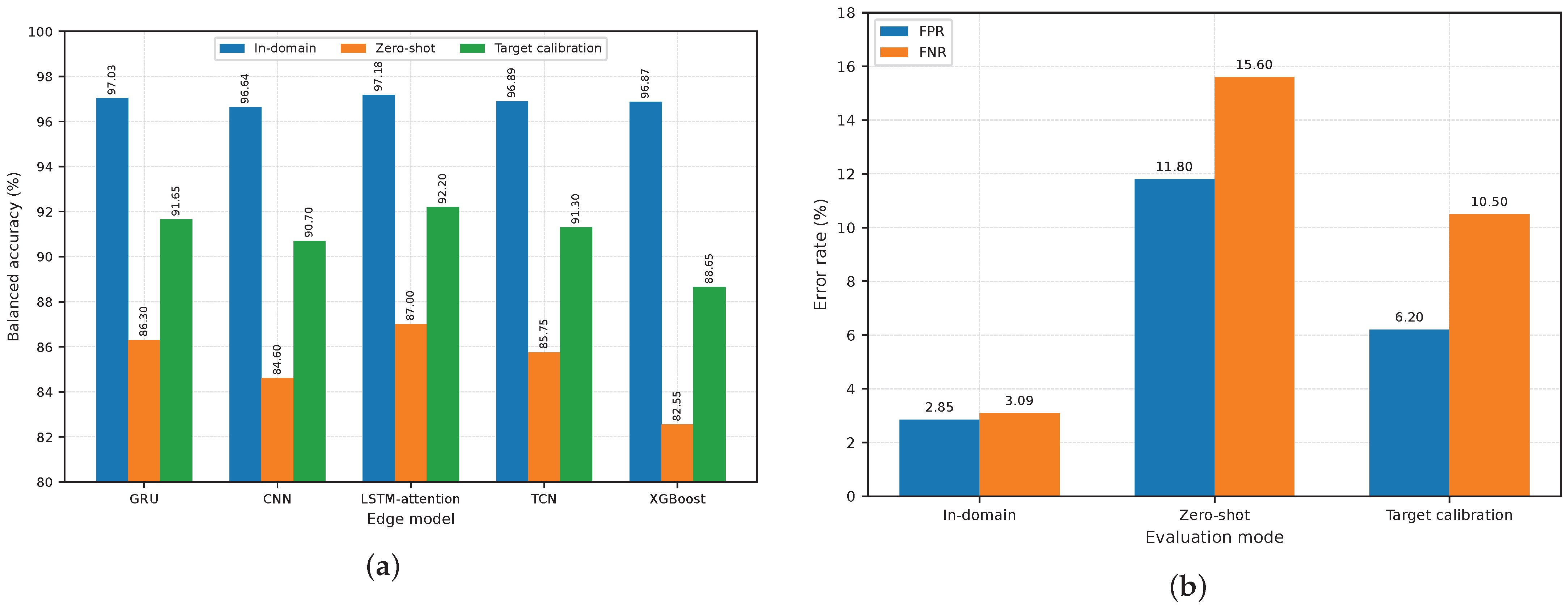
• We compare the GRU implementation with matched causal CNN, LSTM-attention, temporal-convolutional, and XGBoost edge models and assess in-domain, zero-shot, and target-calibration-only performance on CICIDS2017.

The remainder of this paper is organized as follows. Section 2 reviews related work on IoT intrusion detection, early traffic classification, edge–cloud security analytics, calibrated decision-making, and evaluation reliability. Section 3 presents the proposed framework. Section 4 describes the experimental methodology. Section 5 reports the evaluation results. Section 6 discusses on-device deployment at the edge gateway and cross-domain applicability. Section 7 concludes the paper.

2. Related Work

2.1. IoT Intrusion Detection and Edge-Based Security Analytics

Learning-based intrusion detection for IoT networks has been studied across host-based, network-based, centralized, and distributed settings. Existing surveys emphasize that IoT traffic is heterogeneous, device resources are limited, and deployment conditions differ from conventional enterprise networks [1,2,3]. Industrial IoT settings add requirements for availability, latency, and operational continuity, which motivates detection methods that can operate near the monitored process rather than only in a remote cloud service [4].

A common response to endpoint resource constraints is to place detection at an IoT gateway, edge node, or nearby monitoring point. IoT-KEEPER performs online traffic analysis at the edge to identify malicious IoT activity [5]. Kitsune shows that online network intrusion detection can be implemented through an ensemble of autoencoders over traffic features [6]. Other IoT-oriented work has considered distributed deep learning, consumer IoT DDoS detection, and device-specific botnet detection using network behavior [7,8,9]. These studies justify edge or gateway-side monitoring and provide useful evidence for detection near the traffic source. The present study focuses on a different operational question: how an edge gateway should act when only a partial flow has been observed and the available evidence may or may not be sufficient for a reliable decision. In this setting, the gateway must choose between local exit, continued observation, and escalation for additional processing.

2.2. Early and Partial-Flow Intrusion Detection

Early traffic classification has a longer history in network measurement and application identification. Bernaille et al. showed that traffic can be classified using the first packets of a connection, and later work extended this idea to encrypted application recognition [10,11]. Dainotti et al. studied early network traffic classification through classifier combination, while Gupta et al. revisited early application identification using flow-level evidence [12,13]. Related work has also considered timely classification using probabilistic models and compact early-flow representations for encrypted traffic [14,15]. More recent work has examined partial-flow feature extraction for faster network intrusion detection [16].

These studies support the central premise that useful decisions may be possible before complete flow observation. However, early traffic classification and early intrusion detection are not identical operational problems. Application identification can often tolerate a delayed or uncertain class label, whereas intrusion detection must manage asymmetric error costs: premature benign exits can miss attacks, while premature malicious exits can increase false alarms. The proposed framework is therefore positioned around causal packet-prefix evidence and sequential routing decisions rather than around complete-flow feature extraction or a single early-prediction checkpoint.

2.3. Edge–Cloud Intrusion Detection

Cloud, edge, and federated architectures have also been proposed for IoT and cyber–physical intrusion detection. Yang et al. study efficient intrusion detection for IoT networks using cloud–edge collaboration [17]. Federated learning has been used to distribute intrusion-detection training across IoT, agricultural IoT, industrial cyber–physical, and vehicular edge environments [18,19,20]. These studies address important deployment concerns, including where models are trained, how updates are aggregated, and how communication or privacy constraints affect collaborative detection.

The edge–cloud division in the framework is narrower and more decision-oriented. The edge is not only a local feature extractor or a participant in distributed training; it is the first decision point for each flow prefix. The cloud is not used for all traffic or only for global aggregation. Instead, it is invoked selectively for unresolved flows that remain insufficiently reliable under the edge policy. This distinction matters because the cloud training data, cloud inputs, and final evaluation protocol must reflect the same unresolved-flow routing rule used at deployment.

Recent studies have also examined lightweight and collaborative IDS designs for edge-enabled IoT systems. Wardana et al. combine federated learning, trust management, and privacy-preserving coordination in a hierarchical edge–fog–cloud architecture [29], whereas Nedungadi et al. evaluate a lightweight multimodal LGBM–XGBoost ensemble on Raspberry Pi hardware [30]. Although their architectures and evaluation settings differ from the present framework, both studies reinforce the need to consider detection performance together with model complexity, communication requirements, and edge-resource use.

2.4. Calibration, Selective Classification, and Reliability-Aware Decisions

The framework relies on calibrated probabilities and selective routing rather than on raw classifier scores alone. Classical probability-calibration work shows that classifier scores often require post-processing before they can be interpreted as reliable probabilities [21,22]. Modern neural networks can also be miscalibrated, and temperature scaling is a widely used post hoc calibration method [23]. These observations are relevant to early intrusion detection because threshold-based exits depend on probability estimates, not only on ranking quality.

The decision structure also relates to classification with a reject option and selective classification. Reject-option learning formalizes the idea that a classifier may abstain when the prediction is insufficiently reliable [24]. Selective classification studies the risk–coverage trade-off obtained by predicting only on examples that satisfy a confidence condition [25]. The framework adapts this general idea to an edge-gateway intrusion-detection setting with four possible outcomes at each checkpoint: early benign exit, early malicious exit, continued observation, or cloud refinement. The use of separate benign and malicious thresholds reflects the asymmetric consequences of missed attacks and false alarms, rather than treating abstention as a single undifferentiated reject state.

Selective feature fusion has also been studied with lightweight state-space models in other detection domains. Wang et al. use mask-guided Mamba fusion to regulate cross-modal information exchange in visible–infrared vehicle detection [31]. The sensing task and masking mechanism differ from packet-prefix intrusion detection, but the study provides a relevant example of lightweight temporal fusion under selective evidence integration.

2.5. Evaluation Reliability and Dataset Considerations

Evaluation reliability remains a recurring concern in learning-based intrusion detection. Sommer and Paxson argue that intrusion detection differs from many standard machine-learning settings because operational deployment, class imbalance, and changing adversarial behavior complicate evaluation [26]. Ring et al. survey network-based intrusion-detection datasets and document differences in traffic sources, attack coverage, and labeling practices [27]. Dataset-specific analyses also show that experimental conclusions can be distorted by artifacts, leakage, or inconsistent preprocessing; the CICIDS2017 case study is one example of such concerns [28].

These issues are directly relevant to an edge–cloud early-detection framework. If the edge model, probability calibrator, threshold-selection procedure, cloud classifier, and final test set are not separated, the reported benefit of cloud refinement can reflect reuse of information rather than deployment-relevant generalization. In the proposed framework, the cloud stage is therefore fitted using representations that are generated out of sample, such as out-of-fold edge predictions or a separate development partition.

The present study is positioned around a specific operational problem: an IoT edge gateway observes only a partial flow and must decide whether the available evidence is sufficient for a local decision, whether the flow should remain under observation, or whether it should be escalated for cloud refinement. This framing differs from complete-flow IDS, fixed-window IDS, cloud-assisted IDS, and general selective classification because the routing action is tied to causally available packet-prefix evidence at each checkpoint. The proposed framework formalizes this sequential routing problem and defines the associated representation, calibration, escalation, and leakage-control requirements.

3. Proposed Method

This section presents the proposed framework for reliability-aware early intrusion detection in edge–cloud IoT networks. The section first describes the deployment setting and framework workflow, and then formalizes the causal flow representation, edge scoring model, routing policy, cloud-refinement stage, and calibration protocol.

3.1. Overview of the Proposed Framework

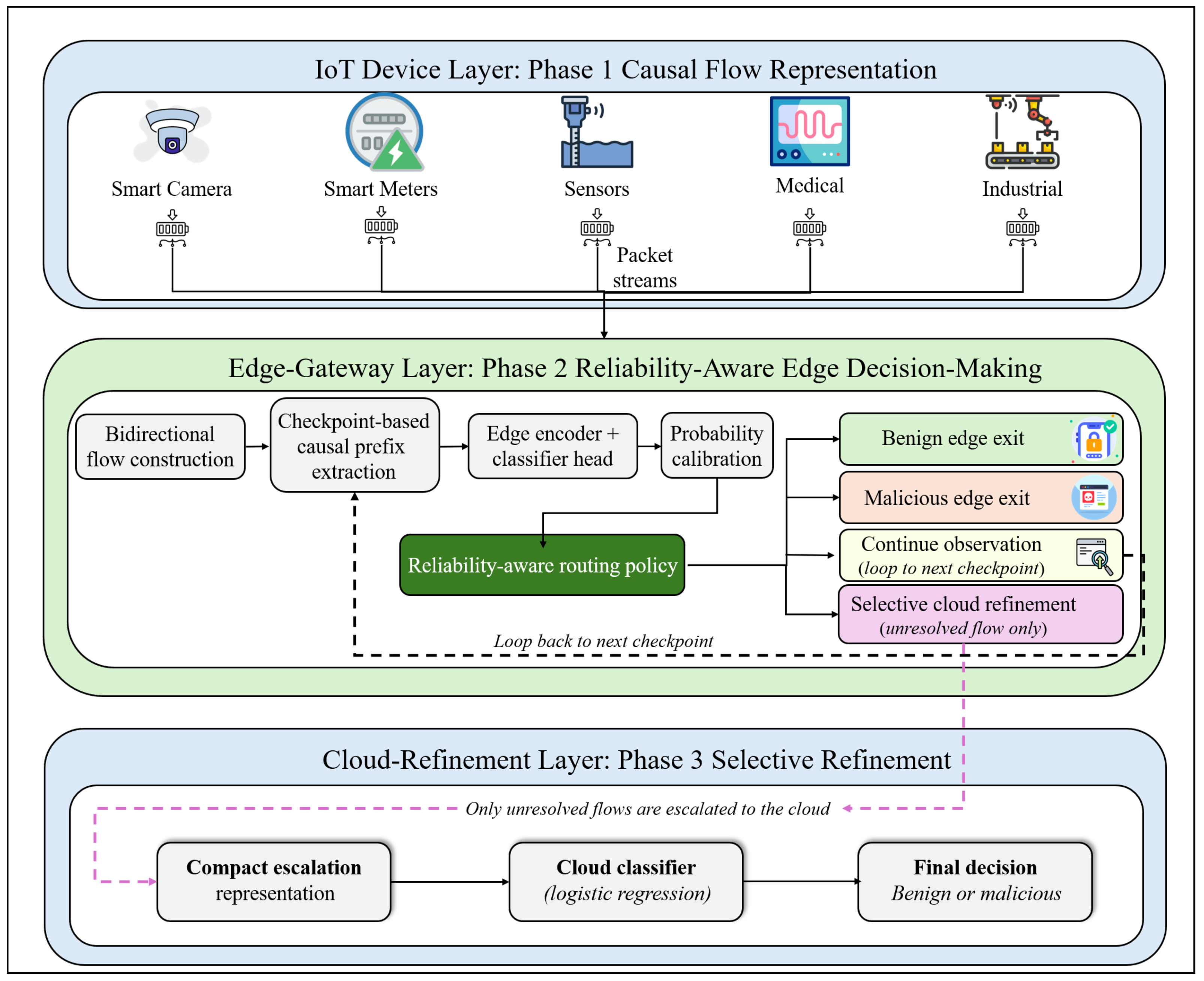
The proposed framework is designed for network-based intrusion detection in IoT deployments where device traffic is observed at an edge gateway and unresolved cases can be refined by a cloud service. The framework consists of three logical layers: the IoT device layer, the edge-gateway layer, and the cloud-refinement layer.

Figure 1 summarizes the proposed reliability-aware edge–cloud IDS workflow. The framework is organized around three connected layers. The IoT device layer provides heterogeneous packet streams from devices such as cameras, smart meters, sensors, medical monitors, and industrial devices. The edge-gateway layer is the primary inference and routing point: it reconstructs bidirectional flows, extracts causal packet prefixes at predefined checkpoints, computes calibrated malicious-probability estimates, and applies the reliability-aware routing policy. The cloud-refinement layer is invoked only for flows that cannot be resolved reliably at the edge.

• Step 1: Packet observation at the edge gateway. IoT devices transmit traffic through the edge gateway. The gateway observes packet-header and timing information from heterogeneous device streams, but the devices themselves are treated only as traffic sources. The framework therefore does not require endpoint-resident IDS models or device-side instrumentation.
• Step 2: Bidirectional flow construction. The gateway groups packets into bidirectional flows using normalized transport-level flow identifiers. Packets from the forward and reverse directions of the same communication are assigned to one flow state. Raw addresses are used only for flow construction and flow verification, not as classifier inputs.
• Step 3: Causal prefix extraction. At each checkpoint, the gateway constructs the currently observed prefix of each active flow. Only packets available up to that checkpoint are used. Complete-flow duration, final packet count, post-flow statistics, labels, scenario identifiers, file identifiers, and other non-causal fields are excluded from the representation.
• Step 4: Edge scoring and probability calibration. The causal prefix is processed by the edge encoder and classifier head to produce an uncalibrated malicious score. This score is converted into a calibrated malicious probability using the calibration mapping. The calibrated probability is the quantity used by the routing policy, rather than the raw classifier score.
• Step 5: Reliability-aware routing. At each checkpoint, the routing policy applies the minimum-evidence condition together with asymmetric benign and malicious thresholds. If the prefix contains sufficient evidence and the calibrated probability falls below the benign threshold, the flow exits locally as benign. If the prefix contains sufficient evidence and the calibrated probability exceeds the malicious threshold, the flow exits locally as malicious. These two edge-exit decisions are therefore allowed only when both the evidence gate and the calibrated threshold condition are satisfied.
• Step 6: Continued observation for unresolved active flows. If an active flow has not yet reached the final available observation point and does not satisfy either edge-exit condition, the gateway keeps the flow under observation until the next checkpoint. This loop prevents uncertain prefixes from being forced into premature benign or malicious decisions.
• Step 7: Selective cloud refinement and final decision. A flow is escalated to the cloud only when it remains unresolved at the final available observation point or when it terminates before satisfying the minimum-evidence requirement. For such flows, the gateway sends a compact escalation representation to the cloud classifier. The cloud classifier then produces the final benign or malicious decision for the unresolved case.

This workflow defines the framework as a sequential reliability-control mechanism rather than as a single-stage classifier. The edge stage resolves only those flows that satisfy calibrated local-exit conditions, while short or uncertain flows are either observed further or selectively escalated. The following subsections formalize the causal representation, edge scoring and calibration procedure, routing policy, cloud-refinement representation, and leakage-control protocol.

3.2. Operational Assumptions and Design Rationale

The framework assumes that packet headers are observable at the IoT edge gateway and that the gateway and cloud service are trusted components of the deployment. Edge–cloud communication is assumed to be protected by the operational infrastructure. Payload-content inspection is not required; the method relies on packet-level metadata and prefix statistics available at the gateway.

The design rationale is based on three considerations. First, complete-flow observation and fixed-window processing can delay decisions for flows whose class is already distinguishable from early evidence. Second, forwarding all flows to the cloud increases communication and processing overhead. Third, early edge decisions require reliability control because premature benign or malicious exits can introduce operational risk.

The framework addresses these considerations through a sequential routing formulation in which prefix-based edge scoring, calibrated reliability-aware routing, and selective cloud refinement are defined as parts of the same decision process. The gateway exits early only when the calibrated score satisfies the benign or malicious decision threshold, and the prefix contains enough packet evidence for a local decision. Otherwise, the flow remains under observation until the next checkpoint or is routed to the cloud at the final available observation point. Offline model training, probability calibration, threshold selection, and cloud-refinement fitting are separated from online inference to avoid tuning the decision process on final test data (

Table 1. Main notation used in the proposed framework formulation.

Symbol	Description
$F_i$	Ordered packet-feature sequence representing flow i.
${\mathbf{x}}_{i,t}$	Packet-level feature vector for the t-th packet of flow i.
$n_i$	Observed length of flow i, measured in packets.
$F_{i,1:t}$	Prefix of flow i observed up to checkpoint t.
$\mathcal{C}$	Set of predefined decision checkpoints.
$L_{\max }$	Maximum observation budget for edge inference.
$m_{\min }$	Minimum packet-evidence requirement before a local edge exit is permitted.
${\overline{L}}_i$	Final available observation point for flow i, defined as $\min (n_i,L_{\max })$.
${\mathcal{C}}_i$	Evaluated checkpoint set for flow i, including checkpoints before ${\overline{L}}_i$ and the final available observation point.
${\varphi }_t(·)$	Feature-transformation function at checkpoint t.
$E_{\theta }$	Causal sequence encoder used by the edge model.
${\mathbf{h}}_{i,t}$	Hidden representation of flow i at checkpoint t.
$f_{\theta }$	Edge classifier head applied to the hidden representation.
$z_{i,t}$	Uncalibrated edge score for flow i at checkpoint t.
$C_{\psi }$	Calibration mapping from edge score to calibrated malicious probability.
$q_{i,t}$	Calibrated probability that the eventual flow label is malicious given prefix $F_{i,1:t}$.
${\tau }_B$	Benign-exit threshold used by the edge routing policy.
${\tau }_M$	Malicious-exit threshold used by the edge routing policy.
$\pi (q_{i,t},t)$	Routing policy that returns an edge decision, continued observation, or cloud refinement.
${\mathbf{r}}_i$	Compact cloud-escalation representation for flow i.
${\mathbf{s}}_{i,{\overline{L}}_i}$	Prefix-only summary statistics at the final available observation point.
$g_{\varphi }$	Cloud-refinement classifier applied to escalated flows.
${\widehat{Y}}_i^c$	Cloud decision for escalated flow i.
${\mathcal{D}}_{\mathrm{cal}}$	Calibration partition used for calibration and threshold selection.
${ϵ}_B,{ϵ}_M$	Calibration-set operating targets for benign-exit and malicious-exit risks.
$R_B,R_M$	Conditional risks associated with benign and malicious early exits.

).

3.3. Causal Packet-Prefix Representation

Packets are grouped into bidirectional flows using the canonical five-tuple consisting of source IP address, destination IP address, source port, destination port, and protocol. Packets in the reverse communication direction are mapped to the same bidirectional flow as the corresponding forward packets. Raw IP addresses are used only for flow construction and are excluded from classifier inputs.

A flow i is represented as an ordered packet-feature sequence

$$F_i=\{{\mathbf{x}}_{i,1},{\mathbf{x}}_{i,2},\dots ,{\mathbf{x}}_{i,n_i}\}.$$

(1)

At checkpoint t, the edge model may access only the observed prefix

$$F_{i,1:t}=\{{\mathbf{x}}_{i,1},\dots ,{\mathbf{x}}_{i,t}\},t\in \mathcal{C}.$$

(2)

The representation is causal if every feature transformation at checkpoint t can be computed from the observed prefix alone:

$${\varphi }_t\left(F_i\right)={\varphi }_t\left(F_{i,1:t}\right).$$

(3)

Thus, features at t cannot depend on packets that arrive after t. Equations (1)–(3) define the admissible causal input at each checkpoint. The edge model in the next subsection can therefore use only packet features and prefix statistics computable from $F_{i,1:t}$.

The label associated with a flow is interpreted at the complete-flow level. An early prediction at checkpoint t therefore estimates the eventual flow label $Y_i$ from partial evidence; it does not assert that the malicious behavior has necessarily appeared before or at packet t. This distinction is important for early intrusion detection because a malicious flow may contain benign-looking prefix traffic before the attack behavior becomes observable. For this reason, the proposed framework records the decision checkpoint together with the decision label and calibrated score. The evaluation protocol should report exit-checkpoint distributions, especially for malicious flows, so that early exits can be interpreted with respect to the amount of observed evidence.

The packet-level representation may include relative arrival time, inter-arrival time, packet direction, packet length, payload length as a numeric length field, time to live or hop limit, protocol, TCP flags, and port category. Prefix statistics may also be used when they are computed only from packets observed so far. The representation excludes raw IP classifier inputs, payload content, dataset identifiers, file identifiers, other non-causal metadata, labels or label-derived fields, complete-flow duration, final packet count, post-flow aggregate statistics, and any other field unavailable at the current checkpoint.

3.4. Edge Prefix Scoring and Calibration

At each checkpoint, the edge model maps the observed prefix to a causal hidden representation, a binary score, and a calibrated malicious probability:

$$\begin{array}{cc}\hfill {\mathbf{h}}_{i,t}& =E_{\theta }\left(F_{i,1:t}\right),\hfill \\ \hfill z_{i,t}& =f_{\theta }\left({\mathbf{h}}_{i,t}\right),\hfill \\ \hfill q_{i,t}& =C_{\psi }\left(z_{i,t}\right).\hfill \end{array}$$

(4)

Here, $E_{\theta }$ is a causal sequence encoder, $f_{\theta }$ is a classifier head, $C_{\psi }$ is the calibration mapping, and $q_{i,t}\in [0,1]$ estimates the probability that the eventual flow label is malicious given only the observed prefix. Equation (4) maps each causal prefix in Equation (2) to the calibrated malicious probability used by the routing policy. The notation uses a generic calibration mapping; the experimental protocol may instantiate it as a shared calibrator or as checkpoint-specific calibrators depending on calibration performance on held-out calibration data.

The stopping policy is independent of the particular causal encoder. Compact recurrent, convolutional, or temporal-convolutional encoders are compatible with this formulation, provided they consume only $F_{i,1:t}$. The experimental instantiation specifies the encoder family and configuration under a common evaluation protocol. The formulation does not require an attention module; attention-based encoding can be evaluated as an alternative causal architecture under the same protocol.

3.5. Reliability-Aware Edge Decision and Routing Policy

The calibrated probability $q_{i,t}$ supports a reliability-aware stopping policy. Let ${\tau }_B$ and ${\tau }_M$ denote benign-exit and malicious-exit thresholds satisfying

$${\tau }_B<0.5<{\tau }_M.$$

Let $m_{\min }$ denote the minimum number of observed packets required before a local edge exit is permitted. This condition prevents the gateway from assigning a final benign or malicious edge decision when the prefix is too short to satisfy the evidence requirement, even if the calibrated probability is near an exit threshold.

Let ${\overline{L}}_i=\min (n_i,L_{\max })$ denote the final available observation point for flow i, where $n_i$ is the observed flow length when the flow terminates naturally. The evaluated checkpoint set for flow i is

$${\mathcal{C}}_i=\{t\in \mathcal{C}:t<{\overline{L}}_i\}\cup \left\{{\overline{L}}_i\right\}.$$

This definition allows the policy to handle both flows that reach the maximum observation budget and flows that terminate before $L_{\max }$. For $t\in {\mathcal{C}}_i$, the policy is

$$\pi (q_{i,t},t)=\left\{\begin{array}{cc}\mathrm{benign},\hfill & t\ge m_{\min },q_{i,t}\le {\tau }_B,\hfill \\ \mathrm{malicious},\hfill & t\ge m_{\min },q_{i,t}\ge {\tau }_M,\hfill \\ \mathrm{continue},\hfill & t<{\overline{L}}_i,\left(t<m_{\min }\mathrm{or}{\tau }_B<q_{i,t}<{\tau }_M\right),\hfill \\ \mathrm{cloud},\hfill & t={\overline{L}}_i,\left(t<m_{\min }\mathrm{or}{\tau }_B<q_{i,t}<{\tau }_M\right).\hfill \end{array}\right.$$

(5)

Using the calibrated probability from Equation (4), the routing policy in Equation (5) determines whether the current prefix is sufficient for an edge decision or whether additional observation or cloud refinement is required. A local benign or malicious exit requires both calibrated threshold support and the minimum evidence condition $t\ge m_{\min }$. Before ${\overline{L}}_i$, a flow that does not satisfy an eligible exit condition remains under observation. At ${\overline{L}}_i$, a flow is routed to cloud refinement if it remains within the uncertain probability band or if it terminates before the minimum evidence requirement is met. Thus, very short unresolved flows are escalated rather than discarded or assigned a default benign label.

Algorithm 1 applies Equation (5) sequentially over the checkpoint set for one flow.

Algorithm 1. Online inference for one flow
Require: flow packet stream; checkpoint set $\mathcal{C}$; maximum observation budget $L_{\max }$; minimum evidence $m_{\min }$; encoder $E_{\theta }$; classifier head $f_{\theta }$; calibrator $C_{\psi }$; thresholds ${\tau }_B,{\tau }_M$; cloud classifier $g_{\varphi }$.
Ensure: decision label; route; decision checkpoint; calibrated score; cloud decision when escalated.
1:	Initialize flow state and prefix buffer.
2:	Set ${\overline{L}}_i$ as the earlier of $L_{\max }$ and the natural end of the flow.
3:	Set ${\mathcal{C}}_i=\{t\in \mathcal{C}:t<{\overline{L}}_i\}\cup \left\{{\overline{L}}_i\right\}$.
4:	for each checkpoint $t\in {\mathcal{C}}_i$ do
5:	Update $F_{1:t}$ using packets observed through t.
6:	Compute ${\mathbf{h}}_t=E_{\theta }\left(F_{1:t}\right)$.
7:	Compute $z_t=f_{\theta }\left({\mathbf{h}}_t\right)$.
8:	Compute $q_t=C_{\psi }\left(z_t\right)$.
9:	if $t\ge m_{\min }$ and $q_t\le {\tau }_B$ then
10:	return benign edge decision, route, checkpoint t, and score $q_t$.
11:	end if
12:	if $t\ge m_{\min }$ and $q_t\ge {\tau }_M$ then
13:	return malicious edge decision, route, checkpoint t, and score $q_t$.
14:	end if
15:	if $t<{\overline{L}}_i$ then continue observing.
16:	end for
17:	Construct the cloud escalation representation $\mathbf{r}$ as defined in Section 3.6.
18:	Compute ${\widehat{Y}}^c=g_{\varphi }\left(\mathbf{r}\right)$.
19:	return cloud decision ${\widehat{Y}}^c$, route, checkpoint ${\overline{L}}_i$, and score $q_{{\overline{L}}_i}$.

Flows reach the cloud route when the final available prefix is either too short for an eligible edge exit or remains within the uncertain calibrated-probability interval. The compact escalation representation $\mathbf{r}$ is defined in the next subsection.

3.6. Selective Cloud Refinement

Only flows satisfying $\pi (q_{i,{\overline{L}}_i},{\overline{L}}_i)=\mathrm{cloud}$ are escalated. This includes flows that remain uncertain at the final available observation point and flows whose final observed prefix is shorter than the minimum evidence requirement. The cloud therefore receives selected cases that are not eligible for a reliable edge exit rather than a random sample of all traffic. For flows assigned to the cloud route by Equation (5), the gateway constructs the compact causal representation

$${\mathbf{r}}_i=\left[{\mathbf{h}}_{i,{\overline{L}}_i},q_{i,{\overline{L}}_i},{\mathbf{s}}_{i,{\overline{L}}_i}\right],$$

(6)

where ${\mathbf{h}}_{i,{\overline{L}}_i}$ is the final available causal prefix embedding, $q_{i,{\overline{L}}_i}$ is the calibrated malicious probability at the final available observation point, and ${\mathbf{s}}_{i,{\overline{L}}_i}$ contains prefix-only statistics. Equation (6) reuses the final prefix embedding and calibrated probability from Equation (4), together with prefix-only summary statistics.

Candidate elements of ${\mathbf{s}}_{i,{\overline{L}}_i}$ include forward packet count, backward packet count, packet-length mean and variance, inter-arrival-time mean and variance, TCP-flag counts, and direction ratio, all computed from packets observed up to ${\overline{L}}_i$. The cloud prediction is

$${\widehat{Y}}_i^c=g_{\varphi }\left({\mathbf{r}}_i\right).$$

(7)

Equation (7) gives the cloud decision for escalated flows. In the experimental instantiation, $g_{\varphi }$ is implemented as a binary classifier over the compact escalation representation; the selected protocol uses logistic regression to avoid unnecessary model complexity at the cloud stage. The representation excludes raw IP addresses, payload contents, dataset identifiers, file identifiers, and unavailable complete-flow statistics. Cloud-stage metrics are conditional on escalation because the escalated subset is selected by the stopping policy.

3.7. Training, Calibration, and Leakage Control

The methodology separates preprocessing, edge-model training, probability calibration, threshold selection, cloud-refinement fitting, and final testing. Preprocessing transformations that learn parameters from data are fitted on training data only and then applied without refitting. The edge model is fitted on training data, the calibration mapping $C_{\psi }$ is fitted on held-out calibration data, and the thresholds ${\tau }_B$ and ${\tau }_M$ are selected on calibration data. The test partition is reserved for final assessment and is excluded from training, calibration, threshold selection, cloud fitting, and architecture selection.

For a candidate threshold pair $({\tau }_B,{\tau }_M)$, let $t_i({\tau }_B,{\tau }_M)$ denote the checkpoint at which flow i first exits at the edge or reaches its final available observation point ${\overline{L}}_i$. For a calibration set ${\mathcal{D}}_{\mathrm{cal}}$, edge coverage can be estimated as

$$\mathrm{Cov}({\tau }_B,{\tau }_M)={\displaystyle \frac{1}{|{\mathcal{D}}_{\mathrm{cal}}|}}\sum _{i\in {\mathcal{D}}_{\mathrm{cal}}}\mathbb{I}\left\{\pi \left(q_{i,t_i({\tau }_B,{\tau }_M)},t_i({\tau }_B,{\tau }_M)\right)\in \{\mathrm{benign},\mathrm{malicious}\}\right\}.$$

(8)

The two conditional risks are

$$\begin{array}{cc}\hfill R_B({\tau }_B,{\tau }_M)& =P\left(Y_i=1\mid \pi \left(q_{i,t_i({\tau }_B,{\tau }_M)},t_i({\tau }_B,{\tau }_M)\right)=\mathrm{benign}\right),\hfill \\ \hfill R_M({\tau }_B,{\tau }_M)& =P\left(Y_i=0\mid \pi \left(q_{i,t_i({\tau }_B,{\tau }_M)},t_i({\tau }_B,{\tau }_M)\right)=\mathrm{malicious}\right).\hfill \end{array}$$

(9)

Threshold selection is posed as a risk-constrained calibration problem:

$$\begin{array}{cc}\hfill \underset{{\tau }_B,{\tau }_M}{\max }& \mathrm{Cov}({\tau }_B,{\tau }_M)\hfill \\ \hfill \mathrm{subject}\mathrm{to}& R_B({\tau }_B,{\tau }_M)\le {ϵ}_B,\hfill \\ \hfill & R_M({\tau }_B,{\tau }_M)\le {ϵ}_M.\hfill \end{array}$$

(10)

For a fixed minimum-evidence value $m_{\min }$, the thresholds used in Equation (5) are selected on the calibration partition. Equation (8) estimates the resulting edge coverage, Equation (9) defines the corresponding benign- and malicious-exit risks, and Equation (10) selects the feasible threshold pair with maximum calibration-set coverage. The realized values on held-out test data are reported separately. The parameters ${ϵ}_B$ and ${ϵ}_M$ are calibration-set operating targets rather than distribution-free bounds, and ${\tau }_B$ and ${\tau }_M$ are not tuned on test data.

Algorithm 2 implements Equation (10) over a candidate threshold grid.

Algorithm 2. Risk-constrained threshold selection on calibration data
Require: calibration predictions $\left\{q_{i,t}\right\}$; labels $\left\{Y_i\right\}$; checkpoint outcomes; minimum evidence $m_{\min }$; candidate threshold grid $\mathcal{G}$; target risks ${ϵ}_B,{ϵ}_M$.
Ensure: selected thresholds ${\tau }_B,{\tau }_M$, or an infeasibility status when no threshold pair satisfies the operating targets.
1:	Initialize feasible set $\mathcal{S}\leftarrow \varnothing$.
2:	for each $({\tau }_B,{\tau }_M)\in \mathcal{G}$ with ${\tau }_B<0.5<{\tau }_M$ do
3:	Apply $\pi (q_{i,t},t)$ to calibration predictions.
4:	Compute $\mathrm{Cov}({\tau }_B,{\tau }_M)$.
5:	Compute $R_B({\tau }_B,{\tau }_M)$.
6:	Compute $R_M({\tau }_B,{\tau }_M)$.
7:	if $R_B({\tau }_B,{\tau }_M)\le {ϵ}_B$ and $R_M({\tau }_B,{\tau }_M)\le {ϵ}_M$ then
8:	Add $({\tau }_B,{\tau }_M)$ to $\mathcal{S}$.
9:	end if
10:	end for
11:	if  $\mathcal{S}=\varnothing$  then
12:	return no feasible threshold pair for the chosen operating targets.
13:	else
14:	Select $({\tau }_B,{\tau }_M)\in \mathcal{S}$ with maximum calibration-set coverage.
15:	return ${\tau }_B,{\tau }_M$.
16:	end if

If Algorithm 2 returns no feasible threshold pair, the requested operating targets are treated as not attainable on the calibration partition. In that case, the framework does not force early edge exits under violated calibration constraints. The deployment must either use a conservative fallback in which uncertain flows are routed to cloud refinement, or select relaxed operating targets that are explicitly reported.

Cloud fitting requires additional leakage control because the cloud model receives edge-generated representations from selected flows. To prevent selection leakage, cloud-training representations are generated out of sample, either through out-of-fold edge prediction or through a separate development partition. Consequently, ${\mathbf{h}}_{i,{\overline{L}}_i}$, $q_{i,{\overline{L}}_i}$, and routing outcomes used for cloud fitting reflect deployed inference behavior rather than in-sample edge outputs.

3.8. Computational Outputs and Method Scope

The proposed framework has six structural properties. First, all edge predictions are made from causal packet prefixes. Second, the observation budget and checkpoint set are configurable experimental design parameters rather than fixed assumptions of the method. Third, early exits are controlled by calibrated risk-aware thresholds and a minimum-evidence condition. Fourth, cloud refinement is selective and applies only to flows assigned to the cloud route. Fifth, cloud fitting uses leakage-aware edge representations. Sixth, the methodology can be instantiated with any causal encoder that satisfies the prefix constraint.

The formulation produces detection decisions, route metadata, checkpoints, calibrated probabilities, and cloud outcomes for escalated flows. These outputs support alerts and logs. Response enforcement, endpoint-resident deployment, online model adaptation, and coordinated multi-flow inference are separate extensions. Generalization to attack families absent from training is an evaluation setting rather than an inherent consequence of the formulation.

4. Experimental Setup and Evaluation Protocol

The evaluation reproduces the operating conditions defined in Section 3 while keeping model development separate from final testing. Because the gateway acts on incomplete flow prefixes, the experiments begin from packet-level traffic reconstructed into bidirectional flows; complete-flow feature tables are excluded from model inputs. The protocol combines a full-corpus CIC-IoT-2023 evaluation under outer PCAP-disjoint folds with observation-horizon analysis, alternative operating points, matched edge-model comparisons, and external validation on CICIDS2017.

4.1. Full CIC-IoT-2023 Corpus and Sampling

The principal evaluation uses all 309 PCAP files in CIC-IoT-2023 [32]: four benign captures and 305 attack captures covering 33 attack types in seven families. Packet parsing and bidirectional flow reconstruction yield 81,253,897 flows, comprising 261,955 benign flows and 80,991,942 attack-labeled flows.

Each reconstructed flow inherits the label of its capture scenario or source file. The public release does not include a bidirectional five-tuple label table that supports exact flow-level matching; the CIC-IoT-2023 labels are therefore treated as scenario-level rather than exact packet- or flow-level ground truth. Raw addresses, file names, capture and scenario identifiers, payload content, and label-derived fields are excluded from model inputs.

All benign flows are retained. Attack-labeled flows are sampled deterministically at approximately 2.5% within PCAP and attack-type strata. When the proportional sample for a capture is below 200 flows, 200 flows are retained if available; a capture containing fewer than 200 flows contributes all available flows. Sampling is performed after flow reconstruction and PCAP assignment, and every selected flow remains intact with all of its packets and prefixes. The resulting modeling corpus contains 2,286,754 flows drawn from all 309 PCAPs (

Table 2. Full CIC-IoT-2023 flow inventory and modeling corpus.

Item	Full Reconstructed Corpus	Modeling Corpus
PCAP files	309	309
Total flows	81,253,897	2,286,754
Benign flows	261,955	261,955
Malicious flows	80,991,942	2,024,799
Malicious prevalence	99.68%	88.54%
Flows with $n_i<8$	58,291,546	1,640,517
Flows with $n_i\ge 8$	22,962,351	646,237
Flows with $n_i\ge 16$	18,452,760	519,322
Flows with $n_i\ge 32$	3,965,190	111,594
Flows with $n_i\ge 64$	1,592,576	44,820

).

Appendix A summarizes the retained support for all 33 attack types and the numbers of flows available at the observation budgets used in the sensitivity analysis.

4.2. Flow Reconstruction and Prefix Generation

Packets are ordered by timestamp and grouped into bidirectional flows using a normalized five-tuple of source address, destination address, source port, destination port, and protocol. Reverse-direction packets are assigned to the same normalized flow as the corresponding forward packets. Raw endpoint addresses are retained only for flow construction and duplicate checking and are not used as classifier inputs.

For a reconstructed flow $F_i$ with packet count $n_i$, the principal edge policy evaluates

$$\mathcal{C}=\{2,4,8,16,32\}$$

under the maximum observation budget

$$L_{\max }=32.$$

The final available checkpoint for a shorter flow is

$${\overline{L}}_i=\min (n_i,L_{\max }).$$

Support through 64 packets is retained for the observation-budget sensitivity analysis, but the principal policy remains limited to 32 packets.

Local edge exits are permitted only after the minimum-evidence requirement

$$m_{\min }=8$$

has been met. Flows with $n_i<8$ are consequently edge-ineligible and are routed to the cloud. The evaluation reports edge-eligible and edge-ineligible populations separately because short flows constitute a large fraction of the corpus (

Table 3. Flow-length and edge-eligibility distribution in the full and modeling corpora.

Flow-Length Group	Full Reconstructed Corpus		Modeling Corpus
	Flows	Percentage	Flows	Percentage
$n_i<8$	58,291,546	71.74%	1,640,517	71.74%
$n_i\ge 8$	22,962,351	28.26%	646,237	28.26%
$n_i\ge 16$	18,452,760	22.71%	519,322	22.71%
$n_i\ge 32$	3,965,190	4.88%	111,594	4.88%
$n_i\ge 64$	1,592,576	1.96%	44,820	1.96%

).

4.3. Observation-Budget and Post-Eight-Packet Delay Evaluation

The selected observation horizon is examined using matched configurations with $L_{\max }=16$, 32, and 64. Their checkpoint sets are $\{2,4,8,16\}$, $\{2,4,8,16,32\}$, and $\{2,4,8,16,32,64\}$, respectively. Each configuration is trained, calibrated, and evaluated independently in the same four outer PCAP-disjoint folds, while the encoder architecture, hidden dimension, causal feature schema, minimum-evidence requirement, threshold-selection rule, and cloud-model class and hyperparameters are held fixed. The 16- and 64-packet configurations are used only for sensitivity analysis and do not alter the principal 32-packet policy.

The comparison reports FPR, FNR, balanced accuracy, edge- and cloud-route shares, the mean edge-exit checkpoint, and the mean number of packets processed at the edge per flow. The final measure includes flows that terminate naturally before the maximum budget and flows that exit at an earlier checkpoint.

Sensitivity to later-arriving post-eight-packet information is assessed on the common set of $\mathrm{39,880}$ malicious flows containing at least 64 packets. Packets 1–8 remain unchanged. For $d\in \{4,8,16,32\}$, the feature vector observed at packet 8 is repeated for the next d positions, after which the original sequence beginning at packet 9 is shifted by d positions and truncated at the evaluated horizon. Model parameters, calibration temperatures, and thresholds remain fixed. This controlled perturbation delays all information after packet 8 while preserving the recorded prefix through the minimum-evidence gate; it does not identify which shifted features carry attack evidence.

4.4. Low-FPR Operating Points and Deployment-Prior Analysis

The principal operating point maximizes reliable edge exits subject to the calibrated benign- and malicious-exit risk targets. Three additional policies examine settings in which benign false alarms carry greater operational cost. Within each outer fold, the most permissive asymmetric threshold pair is selected subject to calibration-set FPR limits of $2\%$, $1\%$, or $0.5\%$. The edge encoder, temperature scaler, minimum-evidence gate, and cloud model remain fixed across these operating points.

Deployment-prior sensitivity is evaluated by applying the measured class-conditional FPR and FNR to assumed malicious-flow prevalences of $10\%$, $1\%$, $0.1\%$, and $0.01\%$. Precision and alert counts are then reported per one million flows. This calculation changes only the assumed class prior; the fitted models and pooled out-of-fold confusion matrix remain unchanged.

4.5. Sliding-Window Threshold Updating

A secondary experiment evaluates supervised threshold adaptation under chronological traffic drift. The replay contains all $\mathrm{261,955}$ pooled benign flows and a deterministic attack-stratified sample of $\mathrm{29,106}$ malicious flows, producing a $10\%$ malicious-flow prevalence across eight ordered traffic blocks. Each flow remains associated with the outer-fold system that generated its out-of-fold prediction. The edge encoder, temperature scaler, and cloud classifier of each fold remain fixed; only that fold’s benign and malicious exit thresholds are updated.

Threshold updating is performed separately for the four fold-specific systems. Within each fold, the procedure starts from that system’s static $1\%$-FPR threshold pair, uses the most recent $\mathrm{50,000}$ adjudicated outcomes assigned to the fold, updates after every $\mathrm{10,000}$ fold-specific flows, and assumes a $\mathrm{10,000}$-flow feedback delay. An update requires at least $\mathrm{40,000}$ benign and 2000 malicious labeled examples in the current window. Candidate threshold pairs are evaluated on the same $0.01$ grid used for static threshold selection, with each threshold restricted to a maximum change of $0.02$ from its preceding value. For every candidate pair, the complete sequential routing policy is reapplied to the current window.

A candidate pair is feasible when ${\tau }_B<0.5<{\tau }_M$, the $95\%$ Wilson upper bound on fold-specific FPR is at most $1.25\%$, and the empirical fold-specific FNR is at most $6\%$. Among the feasible pairs, the pair with the largest edge-exit share is selected. Ties are resolved by the smallest total threshold movement, followed by lower empirical FNR and then lower empirical FPR. The preceding threshold pair is retained when the class-support requirements are not met, or no feasible candidate exists. Predictions from the four fold-specific replay streams are pooled only for the aggregate results reported in Section 5.12. Because the procedure uses delayed adjudicated labels, it represents supervised threshold adaptation rather than unsupervised drift detection.

4.6. Feature Schema and Leakage Controls

All model inputs are restricted to information available at packet arrival or within the causal prefix observed so far. Packet-level features include relative packet time, inter-arrival time, direction, packet length, numeric payload length, protocol indicators, TCP-flag indicators, and port category. Prefix summaries comprise observed packet counts, direction-specific counts, packet-length and inter-arrival statistics, TCP-flag and protocol counts, and direction ratios.

Classifier inputs exclude raw source and destination IP addresses, MAC addresses, payload content, DNS names, HTTP URI or content fields, MQTT topics or messages, dataset and capture identifiers, scenario and file identifiers, binary and attack-type labels, label-derived fields, complete-flow duration, final packet count, post-flow aggregates, and any quantity requiring packets beyond the current checkpoint.

Numerical preprocessing parameters are fitted only on the edge-training data of the corresponding outer fold and are applied unchanged to calibration, cloud-development, and held-out PCAPs. All prefixes from one bidirectional flow remain in a single development role.

4.7. Outer PCAP-Disjoint Evaluation Protocol

The principal evaluation uses four outer PCAP-disjoint folds. Each fold holds out one of the four benign PCAPs and approximately one quarter of the attack PCAPs for final testing. The corresponding test captures are excluded from preprocessing, edge-model fitting, calibration, threshold selection, cloud-model fitting, and hyperparameter selection. Across the four folds, every one of the 309 PCAPs appears in final testing exactly once.

Attack PCAPs are distributed so that all seven attack families occur in every outer fold. Some low-volume attack types are absent from individual folds where source multiplicity does not permit broader allocation, but all 33 attack types are represented in the pooled out-of-fold evaluation.

The remaining flows in each outer development pool are assigned to edge-training, calibration, and cloud-development roles in the relative ratio 50:15:15. Together with the 25% outer test share, these roles correspond to effective overall proportions of 46.875%, 14.0625%, 14.0625%, and 25%. The inner roles are flow-disjoint, and every prefix derived from one flow remains in the same role (

Table 4. Outer PCAP-disjoint test support.

Outer Fold	Test Flows	Benign	Malicious	Attack Types	Held-Out Benign PCAP
Fold 1	567,891	122,891	445,000	31	BenignTraffic.pcap
Fold 2	571,561	55,061	516,500	32	BenignTraffic1.pcap
Fold 3	571,688	58,488	513,200	31	BenignTraffic2.pcap
Fold 4	575,614	25,515	550,099	33	BenignTraffic3.pcap
Pooled out-of-fold	2,286,754	261,955	2,024,799	33	All four

and

Table 5. Development-role support within each outer fold.

Outer Fold	Edge Training	Calibration	Cloud Development	Outer Test
Fold 1	1,074,289	322,287	322,287	567,891
Fold 2	1,071,996	321,598	321,599	571,561
Fold 3	1,071,916	321,575	321,575	571,688
Fold 4	1,069,462	320,839	320,839	575,614

).

4.8. Label Source and Validation Scope

The outer-fold design measures generalization to CIC-IoT-2023 captures that are absent from every model-development stage. By separating complete PCAP files, it removes direct capture reuse between development and final testing and limits dependence on capture-specific traffic patterns.

This design leaves the source-label granularity unchanged. Attack-labeled captures may contain background or mixed traffic, so the principal experiment evaluates capture-level generalization under scenario/file-level labels rather than exact flow-label correctness. Cross-dataset transfer is examined separately on CICIDS2017.

The pooled out-of-fold result covers all 33 attack types and all four benign PCAPs. Its scope is the complete CIC-IoT-2023 source collection; unseen-family and operational-network generalization require separate evidence.

4.9. Mandatory Cloud Lower Bound

Because local exits require $m_{\min }=8$, every flow with $n_i<8$ is assigned to the cloud route. Total cloud load can therefore be decomposed as

$$N_{\mathrm{cloud}}=N_{n_i<8}+N_{\mathrm{eligible},\mathrm{uncertain}},$$

where the first term is the mandatory short-flow population and $N_{\mathrm{eligible},\mathrm{uncertain}}$ contains edge-eligible flows that satisfy neither exit threshold (

Table 6. Mandatory cloud-route lower bounds in the outer test folds.

Outer Fold	${\mathit{n}}_{\mathit{i}}<8$	Benign	Malicious	Maximum Edge-Eligible Share
Fold 1	397,475	77,793	319,682	30.01%
Fold 2	415,538	44,523	371,015	27.30%
Fold 3	414,009	46,805	367,204	27.58%
Fold 4	413,495	20,416	393,079	28.16%
Pooled out-of-fold	1,640,517	189,537	1,450,980	28.26%

).

Short flows account for 71.74% of the pooled population, fixing the maximum possible edge-exit share at 28.26%. The realized route composition is evaluated against these structural bounds.

4.10. Model Fitting, Calibration, and Evaluation Use

Each outer fold has its own edge model, temperature scaler, threshold pair, and cloud-refinement model. The edge model is fitted on the edge-training role, probability calibration and asymmetric threshold selection use the calibration role, and the cloud classifier is fitted on cloud-development flows routed by the fixed edge policy. The held-out PCAPs are evaluated only after all components have been fixed.

The principal analysis pools predictions from the four outer test folds. Detection measures comprise accuracy, precision, recall, F1 score, balanced accuracy, FPR, FNR, AUROC, and AUPRC. Routing measures comprise edge- and cloud-route shares, the mandatory short-flow share, route-specific FPR and FNR, and the decision-checkpoint distribution. Calibration-fit diagnostics comprise expected calibration error, negative log-likelihood, and Brier score computed on the same calibration role used to fit the temperature parameter; they are not presented as independent outer-test calibration estimates.

For an attack group g, representing either one attack type or one attack family, FNR is computed over its pooled out-of-fold attack flows. The associated F1 score uses a deterministic fold-weighted benign reference. Let $A_{gk}$ and $B_k$ denote the attack-group and benign supports in outer fold k, and let $A_g={\sum }_k{A}_{gk}$. The effective benign support is $B_g^{*}=\min (A_g,\mathrm{261,955})$. Every pooled benign prediction is retained with fold weight

$$w_{gk}={\displaystyle \frac{B_g^{*}{A}_{gk}}{A_g{B}_k}},$$

so that the effective benign support and fold proportions match those of the attack group. Reference false-positive counts are weighted sums over the benign predictions and are rounded to the nearest integer for tabulation; they can therefore differ between attack groups even when $B_g^{*}=\mathrm{261,955}$. F1 is computed from the unrounded weighted counts. These are binary one-vs-benign measures rather than multiclass F1 scores.

For the all-cloud and fixed-checkpoint comparators, route assignment is recomputed on the cloud-development role. The all-cloud comparator routes every flow to cloud refinement. A fixed-checkpoint comparator classifies every flow that reaches its designated checkpoint from the calibrated edge probability using a 0.5 decision boundary and routes shorter flows to the cloud. For each comparator, a separate cloud-feature scaler and logistic-regression classifier are fitted on the flows assigned to its cloud route and are then applied to the corresponding held-out test-route flows. The principal cloud classifier is not reused after the route definition changes.

4.11. Experimental Implementation Details

The experimental implementation operationalizes the framework defined in Section 3 using a compact causal sequence model at the edge and a regularized logistic-regression classifier at the cloud stage. The edge model operates on padded packet-prefix sequences with maximum length $L_{\max }=32$. For a checkpoint t, only packets $1,\dots ,t$ are visible to the model; packet positions after t are masked and do not contribute to the hidden-state representation. The input tensor for each mini-batch has shape $B\times 32\times d$, where B is the batch size and $d=26$ is the number of packet-level features after numerical scaling and categorical encoding.

The packet-level edge features used in the implementation are listed in

Table 7. Packet-level causal feature schema used by the edge model.

Feature Group	Implemented Fields
Timing features	Relative packet time; inter-arrival time; normalized packet index within the observed prefix.
Size features	Packet length; payload length as a numeric length field.
Direction feature	Packet direction encoded as forward or backward relative to the normalized bidirectional flow.
Header feature	Time-to-live or hop-limit value when available; otherwise, a missing-value indicator is used.
Protocol indicators	One-hot indicators for TCP, UDP, ICMP, and other protocols.
TCP flag indicators	Binary indicators for SYN, ACK, FIN, RST, PSH, URG, ECE, and CWR flags.
Port-category indicators	Source-port and destination-port categories encoded as well-known, registered, ephemeral, or unavailable.

. All continuous variables are standardized using parameters fitted only on the edge-training partition. Categorical protocol, TCP-flag, and port-category variables are one-hot encoded before model fitting. Raw IP addresses, MAC addresses, payload content, capture identifiers, scenario identifiers, file identifiers, complete-flow duration, final packet count, post-flow aggregate statistics, and label-derived fields are excluded from all classifier inputs. The fitted preprocessing parameters are reused without refitting on the calibration, cloud-development, and final-test partitions.

The edge classifier uses a gated recurrent unit (GRU) as the causal sequence encoder $E_{\theta }$. The GRU has one recurrent layer with hidden dimension 64. For each evaluated checkpoint, the last valid hidden state corresponding to the observed prefix is passed to a classifier head consisting of a dense layer with 32 units, ReLU activation, dropout rate 0.2, and a final linear output producing the uncalibrated malicious logit $z_{i,t}$. Padding positions are masked before hidden-state selection, so naturally short flows do not contribute artificial zero-packet evidence beyond their observed length.

The edge model is trained using weighted binary cross-entropy with logits, with class weights computed from the edge-training partition. Training uses the Adam optimizer with learning rate ${10}^{-3}$, weight decay ${10}^{-5}$, batch size 1024, maximum 50 epochs, and gradient clipping at an ${\ell }_2$-norm of 5.0. A stratified 10% subset of the edge-training partition is reserved as an internal validation split for early stopping. Early stopping uses validation loss with patience 7 and minimum improvement ${10}^{-4}$. The calibration partition is not used for edge-model fitting, model selection, or early stopping.

Probability calibration is performed after edge-model training using temperature scaling. A scalar temperature parameter $T>0$ is fitted on the calibration partition by minimizing negative log-likelihood over held-out calibration logits. The calibrated malicious probability is computed as

$$q_{i,t}=\sigma (z_{i,t}/T),$$

where $\sigma (·)$ is the logistic sigmoid. Threshold selection is then performed on calibrated outputs using the fixed minimum-evidence requirement $m_{\min }=8$. The threshold grid is

$${\tau }_B\in \{0.01,0.02,\dots ,0.49\},{\tau }_M\in \{0.51,0.52,\dots ,0.99\}.$$

The selected operating point is the feasible threshold pair with maximum calibration edge-exit coverage subject to the calibration risk targets ${ϵ}_B={ϵ}_M=0.02$. When several threshold pairs satisfy the same coverage, ties are resolved by selecting the pair with the lower calibration false-negative rate and then the lower calibration false-positive rate.

For each flow assigned to cloud refinement, the cloud input is a compact prefix-derived vector constructed only from information available up to the final observed prefix ${\overline{L}}_i$. The cloud vector concatenates the final available edge hidden representation, the calibrated malicious probability, the raw edge logit, the final checkpoint length, packet-count summaries, byte-count summaries, packet-length statistics, inter-arrival-time statistics, TCP-flag counts, protocol counts, and direction-ratio statistics. The resulting cloud vector contains 97 features: 64 edge-hidden features and 33 prefix-summary or score-derived features. No raw IP addresses, capture identifiers, scenario identifiers, file identifiers, labels, or complete-flow statistics are included in the cloud representation (

Table 8. Main experimental implementation settings.

Component	Setting
Maximum sequence length	$L_{\max }=32$ packets.
Checkpoint set	$\{2,4,8,16,32\}$.
Minimum evidence gate	$m_{\min }=8$ packets.
Edge input tensor	$B\times 32\times 26$.
Edge encoder	One-layer GRU, hidden dimension 64.
Classifier head	Dense 32, ReLU, dropout 0.2, linear output.
Loss function	Weighted binary cross-entropy with logits.
Optimizer	Adam, learning rate ${10}^{-3}$, weight decay ${10}^{-5}$.
Batch size	1024.
Maximum epochs	50.
Early stopping	Validation loss, patience 7, minimum improvement ${10}^{-4}$.
Calibration	Temperature scaling on the calibration partition.
Threshold grid	${\tau }_B=0.01$ to 0.49 and ${\tau }_M=0.51$ to 0.99, step 0.01.
Risk targets	${ϵ}_B={ϵ}_M=0.02$.
Cloud classifier	Logistic regression on compact cloud vector.
Cloud representation	97 features: 64 edge-hidden features and 33 prefix-summary or score-derived features.
Cloud regularization	L2 regularization, $C=1.0$.
Cloud solver	lbfgs, maximum 1000 iterations, class-balanced weighting.
Software	Python (v3.10.12), NumPy (v1.26.4), pandas (v2.2.2), scikit-learn (v1.5.1), PyTorch (v2.3.1), and XGBoost (v2.1.1).
Random seed	2026070501.

).

The cloud classifier is fitted only on the cloud-development partition after the fixed calibrated edge policy determines which flows enter the cloud route. The logistic-regression model uses L2 regularization with $C=1.0$, class-balanced weighting, the lbfgs solver, and a maximum of 1000 iterations. Cloud-feature standardization is fitted only on the cloud-development partition and then applied unchanged to final-test cloud-routed flows.

All experiments use fixed random seeds for deterministic sampling, partitioning, model initialization, mini-batch ordering, and classifier fitting. The implementation uses Python with NumPy, pandas, scikit-learn, and PyTorch. Random seeds are fixed at 2026070501; deterministic PyTorch execution is enabled where supported. No final-test data are used for preprocessing fitting, edge-model fitting, calibration, threshold selection, cloud-model fitting, hyperparameter selection, or operating-point selection.

4.12. Independent Edge-Model Comparison Protocol

The architecture comparison controls the evaluation, calibration, routing, and cloud-refinement protocol while comparing alternative causal edge models. The causal feature schema, observation checkpoints, eight-packet minimum-evidence gate, outer PCAP-disjoint folds, model-specific calibration and threshold selection, and logistic-regression cloud-refinement protocol are retained for every model. The compared encoders are the proposed one-layer GRU, a lightweight causal one-dimensional CNN, a compact one-layer LSTM with additive attention over the observed prefix, a three-block causal temporal convolutional network (TCN), and an XGBoost baseline using causal prefix summaries. Raw identifiers, payload content, and unavailable complete-flow features are excluded from every model.

The neural models expose a 64-dimensional final prefix representation. The XGBoost baseline uses 64 boosting rounds; the additive margin contribution from each round at the final available prefix forms the corresponding 64-dimensional representation block, and the sum of these contributions together with the fixed base margin gives the raw XGBoost logit. For every model, this 64-dimensional representation is concatenated with the same 33 score-derived and causal prefix-summary features, yielding a 97-feature cloud vector. A separate logistic-regression cloud classifier is fitted for each edge model on its own route-matched cloud-development flows.

Implementation cost is measured on a Raspberry Pi 5 with 8 GB RAM (Raspberry Pi Ltd., Cambridge, UK) and 64-bit Ubuntu 22.04.4 LTS using one CPU thread, batch size one, and streaming causal inference. Each measurement follows 1000 warm-up flows and covers 10,000 test flows. Reported latency spans a complete 32-packet edge pass. Neural models use float32 storage without acceleration or post-training quantization. Because the logistic-regression cloud-stage model class is common to all systems, it is excluded from the edge-model size and latency comparison.

4.13. CICIDS2017 External-Validation Protocol

CICIDS2017 provides raw PCAP traffic together with labeled flow records containing timestamps, endpoint addresses, ports, protocols, and attack labels [33]. Bidirectional flows are reconstructed from the PCAPs and matched to the released labels by protocol, endpoint pair, ports, and temporal overlap; ambiguous, duplicate, and unresolved matches are excluded. The released complete-flow feature columns are not used as classifier inputs. Instead, the same 26 causal packet-level features used for CIC-IoT-2023 are generated, and the documented attacks are collapsed into the malicious class.

The retained joined corpus contains $\mathrm{2,742,856}$ flows, of which $\mathrm{2,204,219}$ are benign and $\mathrm{538,637}$ are malicious. Balanced modeling retains all malicious flows and a deterministic attack-day-stratified sample of $\mathrm{538,637}$ benign flows, giving $\mathrm{1,077,274}$ flows. The fixed development and test roles are listed in

Table 9. Fixed CICIDS2017 balanced modeling partitions.

Role	Benign	Malicious	Total
Edge training	269,319	269,319	538,638
Calibration	80,796	80,796	161,592
Cloud development	80,796	80,796	161,592
Fixed test	107,726	107,726	215,452

. All external-validation modes use the same untouched test set of $\mathrm{107,726}$ benign and $\mathrm{107,726}$ malicious flows.

After the outer-fold comparison fixes the architecture and hyperparameters, one transfer-source system is fitted for each edge-model family on the complete CIC-IoT-2023 modeling corpus. The corpus is repartitioned deterministically into flow-disjoint edge-training, calibration, and cloud-development roles in the normalized proportions 62.5%, 18.75%, and 18.75%, corresponding to the same relative 50:15:15 development-role ratio used inside each outer fold and preserving PCAP and attack-type strata. This transfer-source fit is separate from, and is not included in, the pooled CIC-IoT-2023 out-of-fold result. Its preprocessing parameters, edge model, temperature, thresholds, cloud-feature scaler, and cloud classifier are then fixed for external evaluation.

The external study separates three modes. In-domain evaluation develops every model component from the CICIDS2017 training, calibration, and cloud-development roles. Zero-shot evaluation applies the corresponding single CIC-IoT-2023 transfer-source system without using CICIDS2017 before testing. Target-calibration-only evaluation retains the transfer-source preprocessing, edge model, cloud-feature scaler, and cloud-classifier coefficients and refits only the temperature and exit thresholds on the CICIDS2017 calibration role. The fixed CICIDS2017 test set is excluded from fitting and operating-point selection in all three modes.

4.14. Valuation Scope and Reproducibility Controls

Corpus reconstruction, deterministic sampling, outer-fold assignment, flow-level role assignment, flow-length accounting, and mandatory cloud-route bounds are fixed before model fitting. The resulting checks confirm that every sampled flow belongs to one outer test fold, no held-out PCAP appears in the corresponding development pool, and all prefixes from one flow remain in a single role.

The principal result consequently represents PCAP-disjoint validation across the complete 309-PCAP CIC-IoT-2023 source collection. Its interpretation remains conditioned on scenario/file-level labels rather than exact flow-level annotation. Low-prevalence behavior, cross-dataset transfer, and attack-specific performance are examined in their dedicated analyses rather than inferred from the aggregate result. Because the principal summaries pool the four held-out folds, they characterize corpus-level out-of-fold performance; fold-level dispersion and statistical uncertainty across PCAP allocations are not estimated.

5. Results

5.1. Evaluation Overview and Metric Definitions

The principal evaluation is based on pooled out-of-fold predictions from the four outer PCAP-disjoint test folds defined in Section 4.7. The pooled population contains $\mathrm{2,286,754}$ flows, comprising $\mathrm{261,955}$ benign flows and $\mathrm{2,024,799}$ attack-labeled flows. Because the malicious prevalence is $88.54\%$, aggregate measures are interpreted together with class-conditional error rates and the deployment-prior analysis. An all-malicious rule would attain $88.54\%$ accuracy on this corpus but only $50\%$ balanced accuracy, with $100\%$ FPR and $0\%$ FNR; accuracy alone is therefore not an informative baseline.

Benign traffic is treated as the negative class and malicious traffic as the positive class. True negatives and false positives are therefore counted over benign flows, whereas true positives and false negatives are counted over malicious flows. The false-positive and false-negative rates are

$$\mathrm{FPR}={\displaystyle \frac{\mathrm{FP}}{\mathrm{FP}+\mathrm{TN}}},\mathrm{FNR}={\displaystyle \frac{\mathrm{FN}}{\mathrm{FN}+\mathrm{TP}}}.$$

Recall is $1-\mathrm{FNR}$, specificity is $1-\mathrm{FPR}$, and balanced accuracy is the mean of recall and specificity. These definitions are used throughout this section.

Routing measures are reported in addition to detection measures because each flow is assigned either to an edge exit or to cloud refinement. The cloud route contains both flows that terminate before the minimum-evidence requirement and edge-eligible flows that remain unresolved. Route-specific FPR and FNR are computed from the benign and malicious supports within each selected route and are therefore interpreted conditionally.

Calibration-fit quantities are obtained from the calibration role of each fold and are used only for probability scaling and operating-point selection. Final detection and routing measures are computed on the corresponding held-out PCAPs and then pooled. The lower-FPR and deployment-prior analyses retain the same class-conditional errors while examining different operating preferences or traffic priors.

5.2. Routing Composition and Principal End-to-End Result

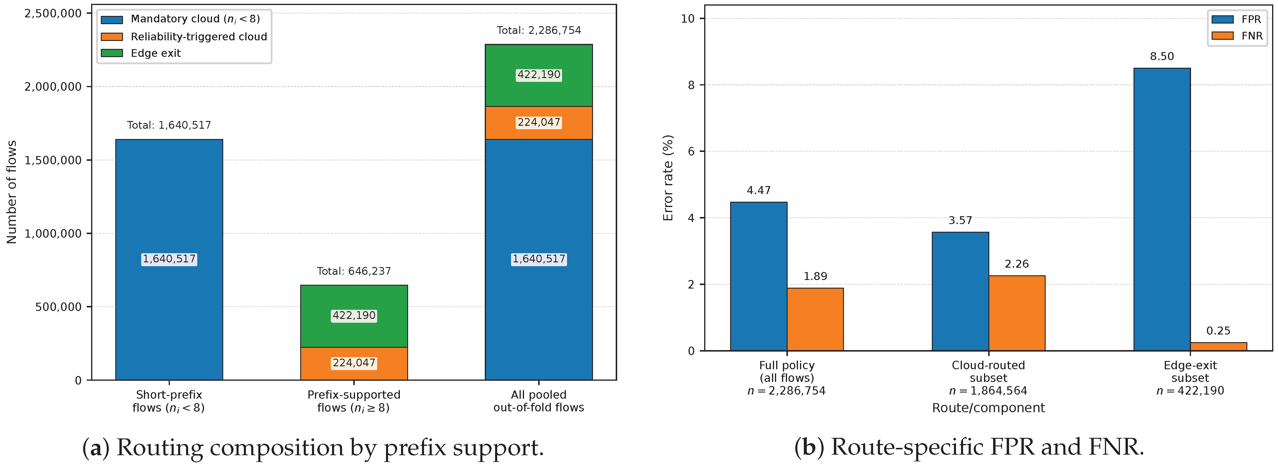
The pooled evaluation contains $\mathrm{2,286,754}$ flows, including $\mathrm{261,955}$ benign and $\mathrm{2,024,799}$ malicious flows. The minimum-evidence gate assigns $\mathrm{1,640,517}$ flows with $n_i<8$ to mandatory cloud refinement. Among the $\mathrm{646,237}$ edge-eligible flows, $\mathrm{422,190}$ satisfy an edge-exit condition and $\mathrm{224,047}$ remain unresolved. The final route composition is therefore $\mathrm{422,190}$ edge exits and $\mathrm{1,864,564}$ cloud-routed flows, corresponding to an edge-exit share of $18.46\%$.

The principal confusion matrix is given in

Table 10. Principal pooled PCAP-disjoint confusion matrix.

Actual Class	Predicted Benign	Predicted Malicious	Total
Benign	250,247	11,708	261,955
Malicious	38,268	1,986,531	2,024,799
Total	288,515	1,998,239	2,286,754

. The end-to-end policy attains $4.47\%$ FPR, $1.89\%$ FNR, $95.53\%$ specificity, and $96.82\%$ balanced accuracy. The remaining false-positive rate is still operationally important in benign-dominated traffic and is examined further through lower-FPR operating points and deployment-prior analysis.

Table 11. Route-stratified pooled detection results.

Route	Support	Benign	Malicious	TN	FP	FN	TP	FPR (%)	FNR (%)	Bal. Acc. (%)
Edge exit	422,190	48,000	374,190	43,920	4080	936	373,254	8.50	0.25	95.63
Cloud-routed	1,864,564	213,955	1,650,609	206,327	7628	37,332	1,613,277	3.57	2.26	97.09
All flows	2,286,754	261,955	2,024,799	250,247	11,708	38,268	1,986,531	4.47	1.89	96.82

separates the selected route populations. The edge-exit subset has $0.25\%$ FNR and $8.50\%$ FPR, whereas the cloud-routed subset has $2.26\%$ FNR and $3.57\%$ FPR. These values describe the error profile of each route after policy selection: the cloud subset contains all short flows and the edge-eligible cases that remain unresolved, while the edge subset contains only flows that satisfy a calibrated exit condition.

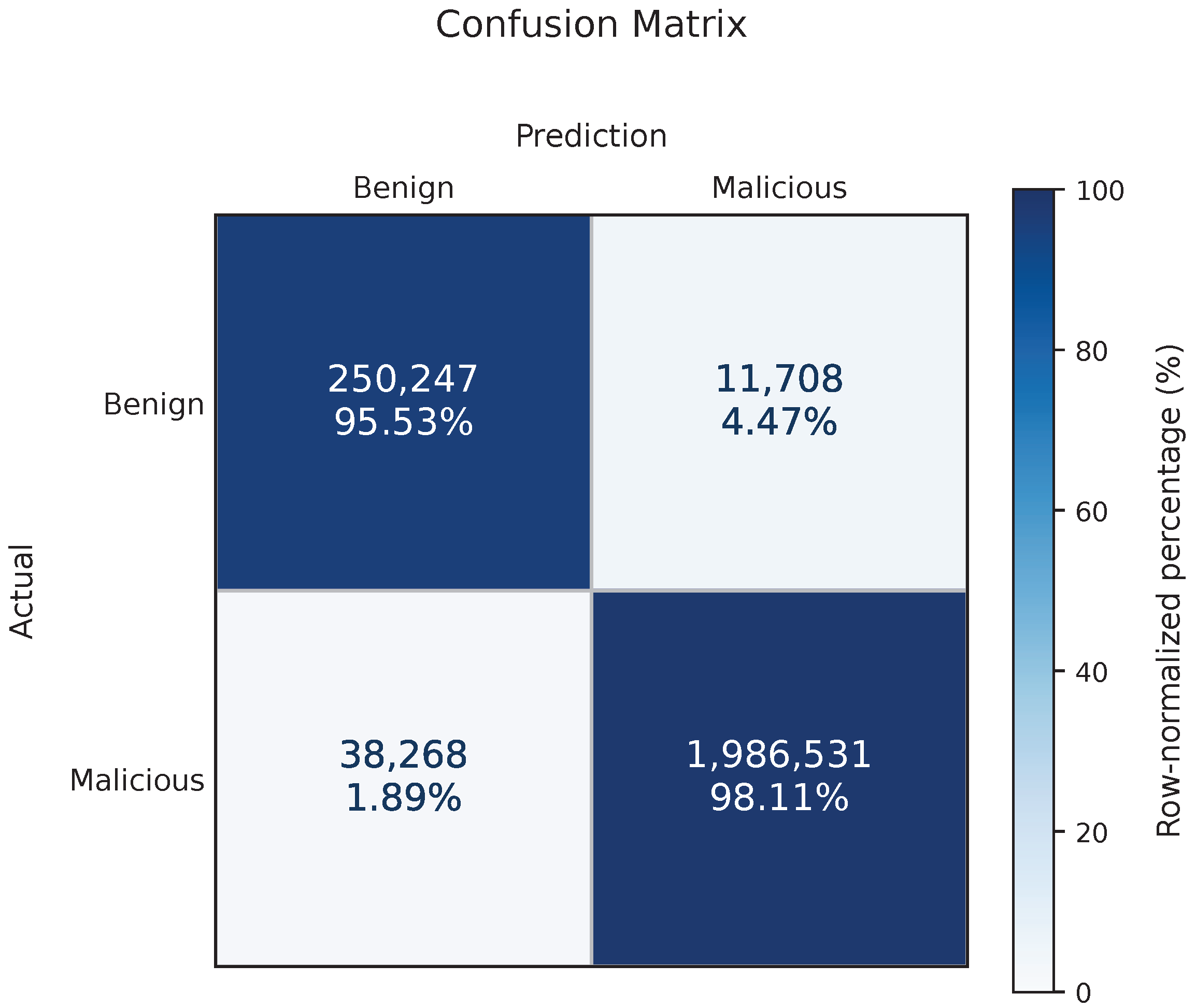
Figure 2 makes the structural cloud lower bound explicit and separates it from reliability-triggered escalation. Figure 3 then shows that the pooled result is not an artifact of the dominant malicious class: the benign row retains $95.53\%$ specificity, while the malicious row retains $98.11\%$ recall.

5.3. Low-FPR Operating Points

Table 12. Static operating points under progressively stricter benign-FPR constraints.

Policy	FP	FN	FPR (%)	FNR (%)	Bal. Acc. (%)	Edge Share (%)	Cloud Share (%)
Principal static	11,708	38,268	4.47	1.89	96.82	18.46	81.54
Validation FPR $\le 2\%$	5239	53,657	2.00	2.65	97.68	16.89	83.11
Validation FPR $\le 1\%$	2620	71,880	1.00	3.55	97.72	15.37	84.63
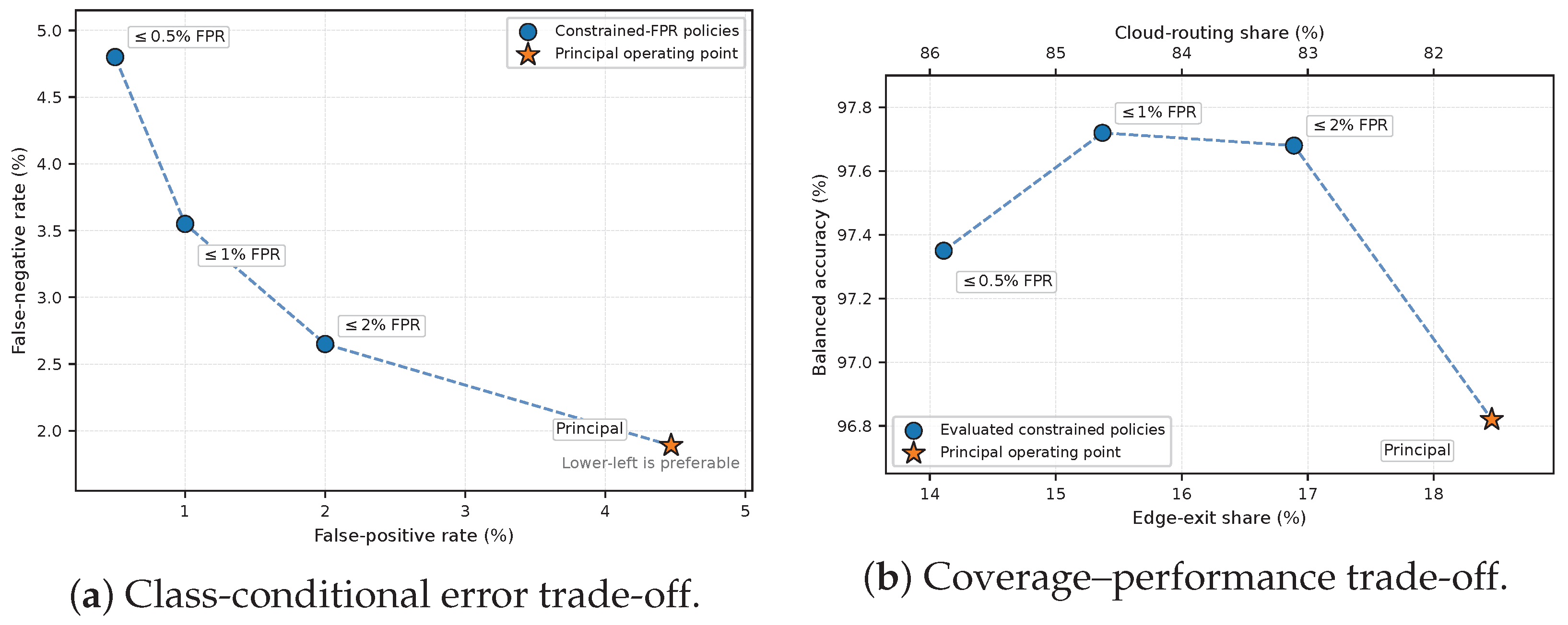
Validation FPR $\le 0.5\%$	1310	97,190	0.50	4.80	97.35	14.11	85.89

reports the principal policy together with three operating points selected under progressively stricter benign-FPR limits. Lower FPR requires more conservative thresholds, which route more flows to the cloud and increase FNR. The $1\%$-FPR policy gives the highest balanced accuracy among the listed settings, but its $3.55\%$ FNR exceeds the malicious-error level of the principal policy. The four settings therefore represent different allocations of benign false alarms, malicious misses, and cloud load.

Figure 4 shows that a lower benign FPR is obtained through a joint change in malicious misses and cloud load rather than through a free improvement in all metrics. The $1\%$-FPR policy has the highest balanced accuracy among the four listed points, but it more than doubles FNR relative to the principal policy.

5.4. Calibration-Based Operating-Point Selection

Threshold selection is performed independently within each outer fold. The principal policy chooses the most permissive asymmetric thresholds that satisfy the calibrated benign- and malicious-exit risk targets together with the minimum-evidence gate. The lower-FPR policies add calibration-set FPR limits of $2\%$, $1\%$, and $0.5\%$, as defined in Section 4.4. Because the fitted temperatures and score distributions differ across folds, each fold has its own selected threshold pair.

The pooled outcomes in Table 12 show the resulting trade-off. Greater protection of benign traffic lowers FPR but increases FNR and cloud routing. The operating point should therefore be selected according to the relative cost of false alarms, missed attacks, and cloud refinement in the intended deployment.

5.5. Calibration-Fit Diagnostics and Discrimination Evidence

Temperature scaling is fitted after edge-model training within each outer fold.

Table 13. Fold-specific temperature-scaling fit diagnostics on the calibration roles.

Fold	Temperature	ECE Raw (%)	ECE Calibrated (%)	NLL Raw	NLL Calibrated	Brier Raw	Brier Calibrated
Fold 1	1.36	4.72	1.28	0.124	0.097	0.031	0.025
Fold 2	1.42	4.95	1.35	0.128	0.099	0.033	0.026
Fold 3	1.39	4.81	1.30	0.126	0.098	0.032	0.026
Fold 4	1.45	4.99	1.33	0.129	0.100	0.033	0.027
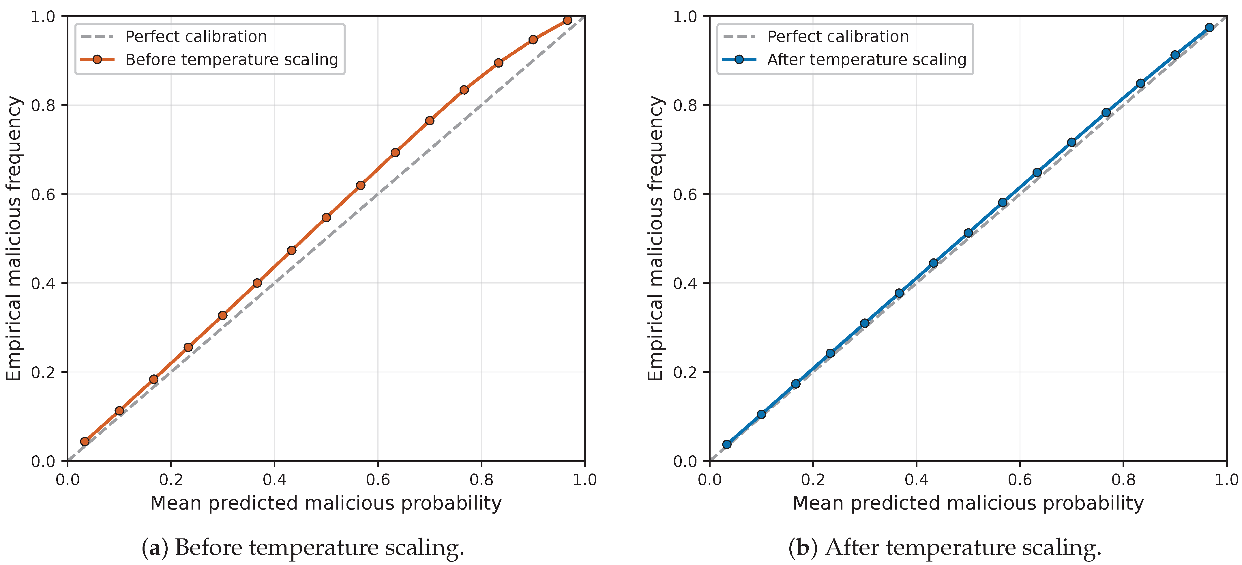
Pooled	1.41	4.86	1.31	0.127	0.099	0.032	0.026

reports the fitted temperatures and within-calibration fit diagnostics. The temperatures range from 1.36 to 1.45. On the same calibration roles used to fit the temperature, pooled ECE decreases from $4.86\%$ to $1.31\%$, NLL from 0.127 to 0.099, and Brier score from 0.032 to 0.026. These values describe the fitted probability mapping used for threshold selection; they are not independent evidence of outer-test calibration. The minimum-evidence gate separately determines whether a prefix is eligible for an edge exit.

Threshold-independent discrimination is reported in

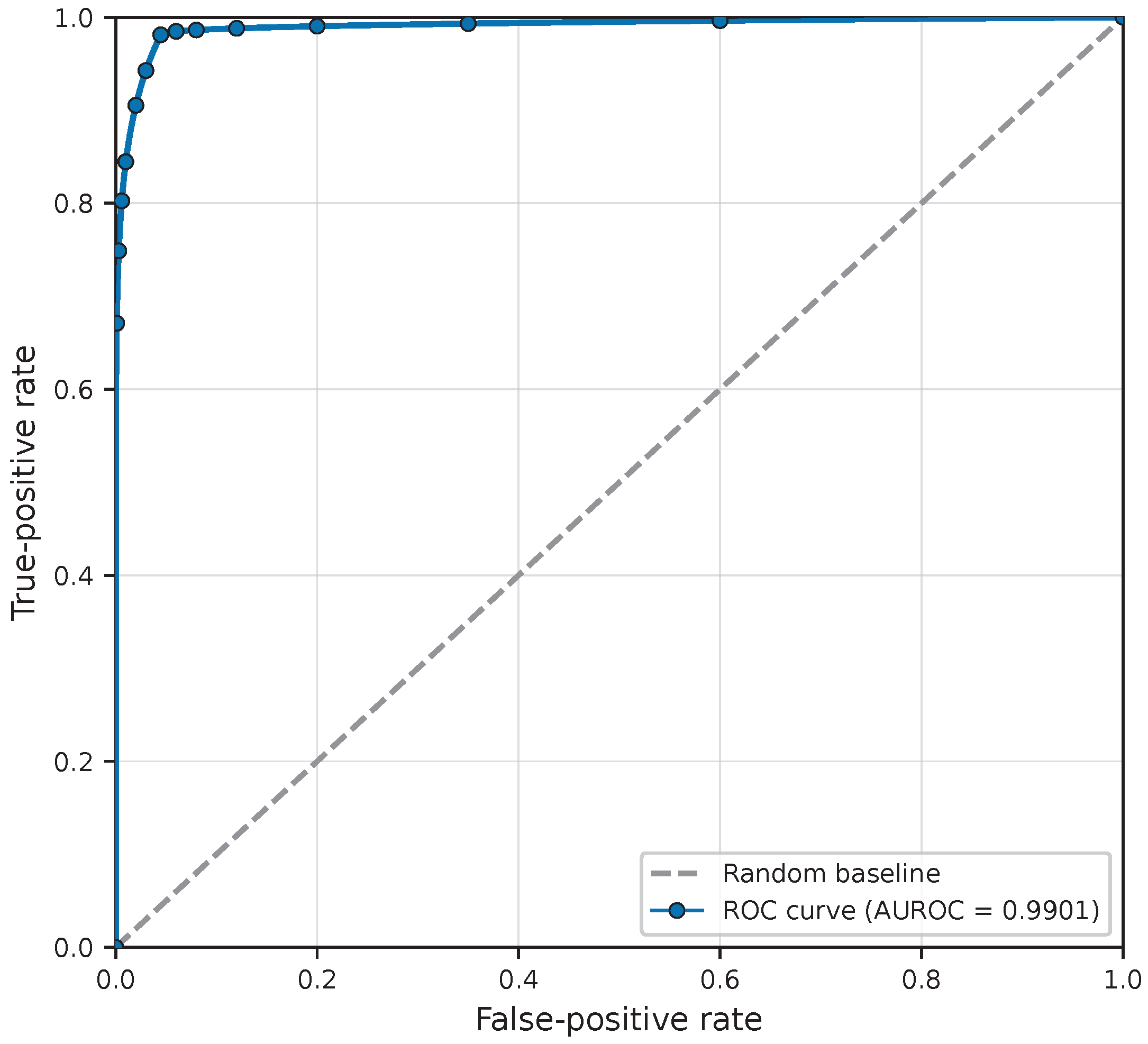
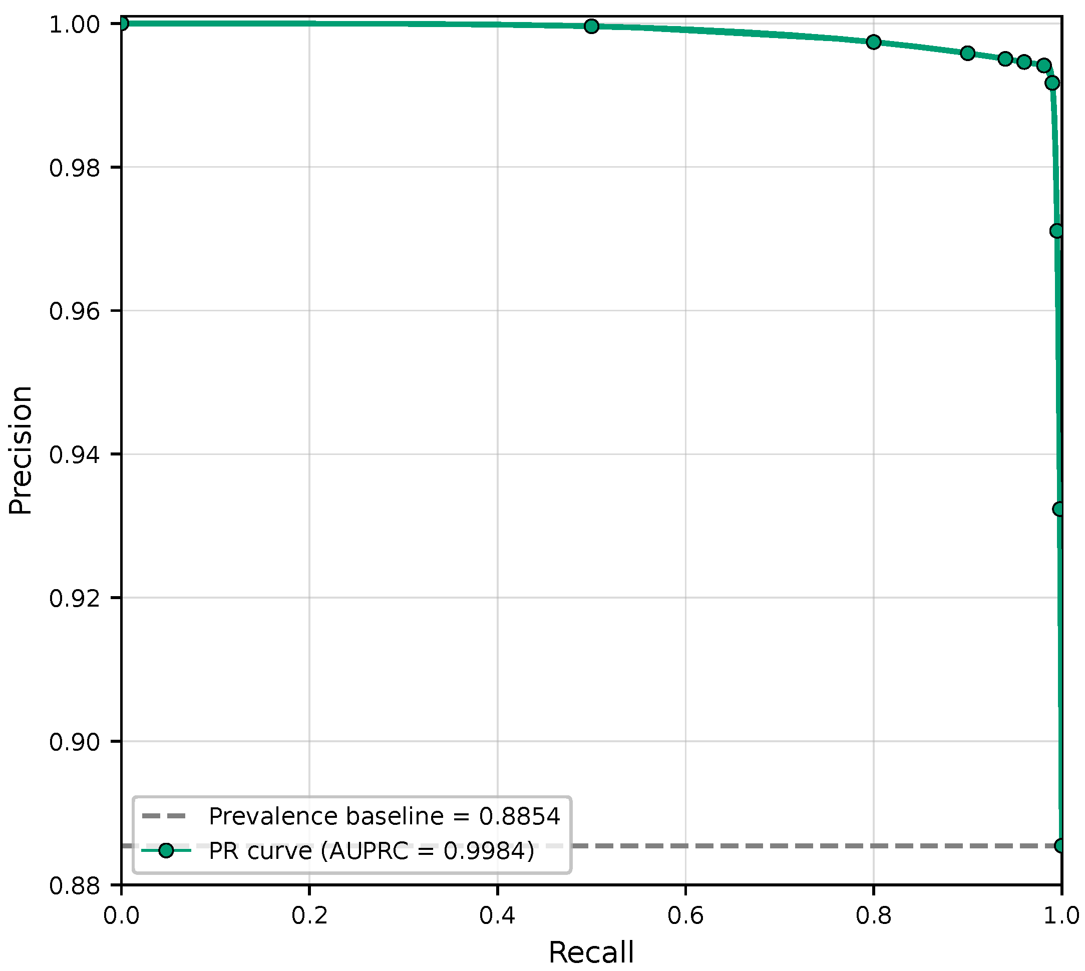
Table 14. Threshold-independent discrimination on pooled out-of-fold predictions.

Evaluation Subset	Support	AUROC	AUPRC
Edge GRU, $n_i\ge 8$	646,237	0.9872	0.9978
Cloud-routed flows	1,864,564	0.9824	0.9971
Final end-to-end scores	2,286,754	0.9901	0.9984

. The edge-eligible GRU scores attain 0.9872 AUROC and 0.9978 AUPRC, the cloud-routed scores attain 0.9824 and 0.9971, and the final end-to-end scores attain 0.9901 and 0.9984 over all $\mathrm{2,286,754}$ flows. The high AUPRC reflects, in part, the $88.54\%$ malicious prevalence and is therefore considered together with FPR, FNR, and the deployment-prior results.

Figure 5, Figure 6 and Figure 7 separate calibration-fit diagnostics from held-out ranking performance. Temperature scaling improves the fitted probability scale used for routing, whereas AUROC and AUPRC characterize threshold-independent discrimination on pooled outer-test predictions. The latter remain high, but AUPRC is interpreted with the observed $88.54\%$ malicious prevalence.

5.6. Route Load and Communication Accounting

Table 15. Route-load and edge-exit checkpoint profile under the principal policy.

Route Component	Flows	All-Flow Share (%)	Edge-Exit Share (%)
Edge exit at packet 8	264,348	11.56	62.61
Edge exit at packet 16	109,842	4.80	26.02
Edge exit at packet 32	48,000	2.10	11.37
All edge exits	422,190	18.46	100.00
Mandatory cloud, $n_i<8$	1,640,517	71.74	–
Unresolved cloud, $n_i\ge 8$	224,047	9.80	–
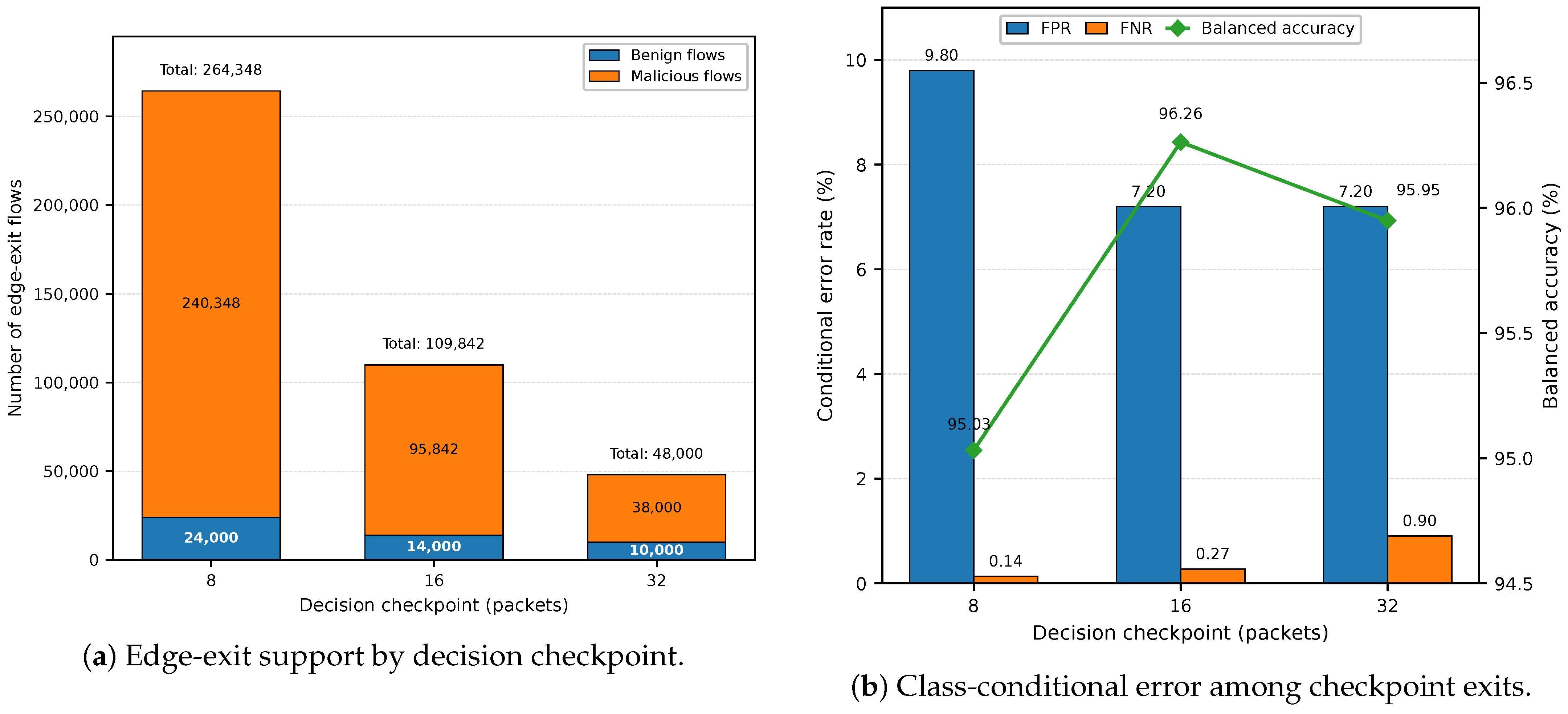
All cloud-routed flows	1,864,564	81.54	–

shows where the final routing decisions occur. The $\mathrm{1,640,517}$ flows shorter than eight packets form the mandatory cloud population, and a further $\mathrm{224,047}$ edge-eligible flows remain unresolved. The remaining $\mathrm{422,190}$ flows exit at packets 8, 16, or 32.

The weighted mean checkpoint among edge exits is 12.81 packets. Packet 8 accounts for $62.61\%$ of all edge exits, while packets 16 and 32 resolve progressively smaller portions of the remaining population. The checkpoint profile therefore shows that most local decisions occur at the first eligible point, with later checkpoints recovering additional unresolved flows.

The communication calculation in

Table 16. Feature-vector communication accounting under the principal policy.

Setting	Cloud Flows	Features	Bytes/Flow	Payload
All-cloud submission	2,286,754	97	388	846.16 MiB
Selective edge–cloud policy	1,864,564	97	388	689.94 MiB
Avoided submissions	422,190	–	–	156.22 MiB
Relative reduction	18.46%	–	–	18.46%

assumes one 97-feature float32 vector for each cloud-routed flow. Relative to submitting the same representation for every flow, selective routing avoids $\mathrm{422,190}$ submissions and reduces the feature payload by $156.22$ MiB, or $18.46\%$, over the pooled evaluation. The calculation excludes serialization, protocol headers, encryption, retransmissions, batching, and control traffic and therefore represents payload accounting rather than a measured network or energy cost (

Table 17. Model-size and representation-size proxy for edge and cloud stages. Parameter counts are reported for the implementation described in Section 4.11.

Quantity	Value	Interpretation
Edge input tensor per flow	$32\times 26$	Maximum padded packet-prefix tensor
Edge input size, float32	3328 bytes	Full padded edge tensor before batching
Cloud vector length	97 features	Compact representation for escalated flows
Cloud vector size, float32	388 bytes	Payload proxy per cloud-submitted flow
Edge GRU hidden dimension	64	Final hidden representation size
Approximate edge-model parameters	19,777	GRU encoder and classifier head
Cloud-model parameters	98	Logistic-regression weights and intercept

).

Figure 8 adds checkpoint-conditional error information to the route counts in Table 15. The exits at packets 8, 16, and 32 have FPRs of $9.80\%$, $7.20\%$, and $7.20\%$, respectively, and FNRs of $0.14\%$, $0.27\%$, and $0.90\%$. These values are conditioned on the flows that first satisfy an exit rule at each checkpoint and therefore should not be compared as if the checkpoint populations were identical.

5.7. Ablation Analysis

Table 18. Ablation results for the principal routing and reliability controls.

Policy Variant	FPR (%)	FNR (%)	Bal. Acc. (%)	Edge Share (%)
Final policy	4.47	1.89	96.82	18.46
No minimum-evidence gate	18.70	4.02	88.64	63.28
No cloud refinement	10.42	4.36	92.61	18.46
Symmetric thresholds	7.68	3.18	94.57	20.24
No temperature scaling	6.36	2.57	95.54	19.11
No benign edge exit	3.71	1.79	97.25	14.36
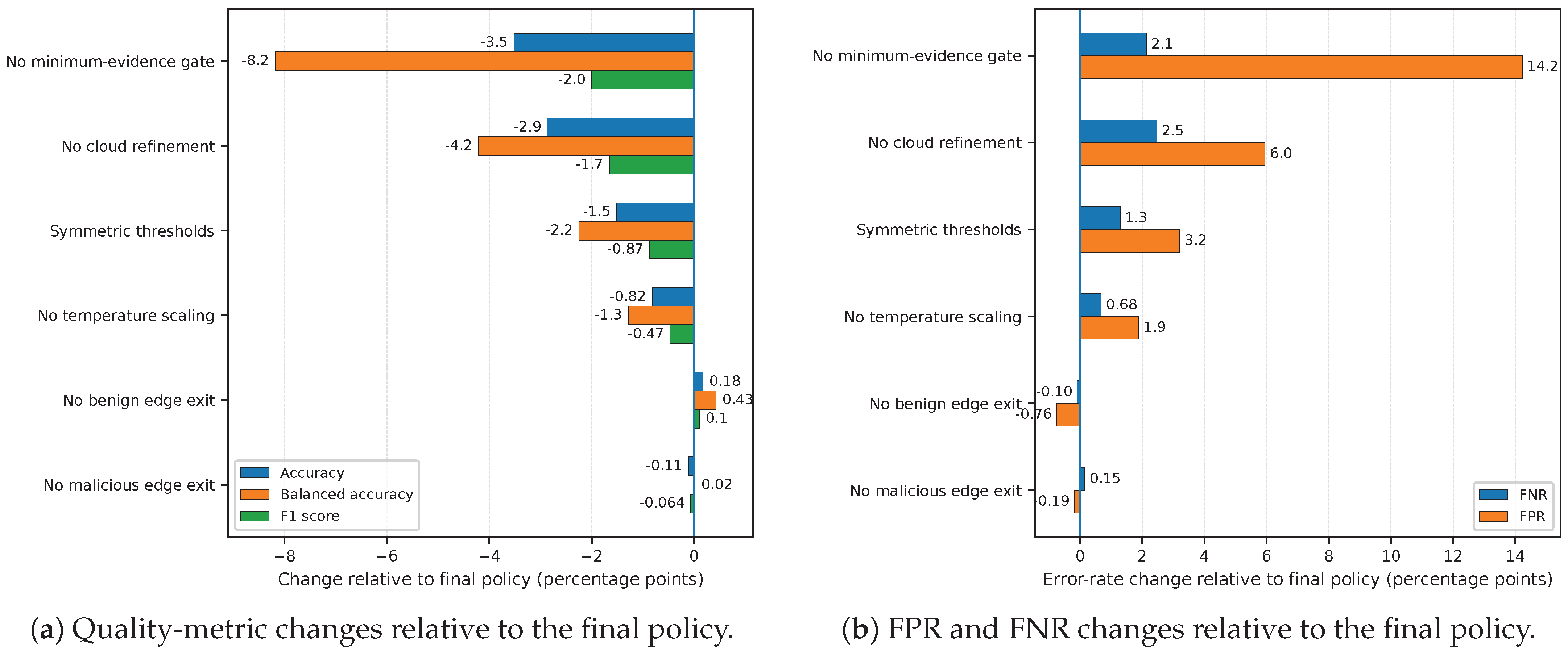
No malicious edge exit	4.28	2.04	96.84	4.10

evaluates the principal reliability and routing components on the pooled PCAP-disjoint predictions. Removing the minimum-evidence gate produces the largest degradation: FPR increases to $18.70\%$, FNR to $4.02\%$, and balanced accuracy falls to $88.64\%$. Removing cloud refinement reduces balanced accuracy to $92.61\%$. Symmetric thresholds and uncalibrated scores also worsen both class-conditional error rates, although their effects are smaller.

The one-sided exit ablations separate detection quality from local coverage. Removing benign edge exits lowers FPR and slightly improves balanced accuracy, but reduces the edge-exit share from $18.46\%$ to $14.36\%$. Removing malicious edge exits leaves balanced accuracy nearly unchanged while reducing local coverage to $4.10\%$. Both exit directions are therefore retained to reduce cloud submissions under the selected reliability policy, rather than because each direction independently maximizes balanced accuracy.

Figure 9 expresses the same ablations relative to the final policy. The result distinguishes reliability controls that prevent large error increases from exit-direction choices that mainly redistribute local coverage.

5.8. Cloud-Refinement Contribution

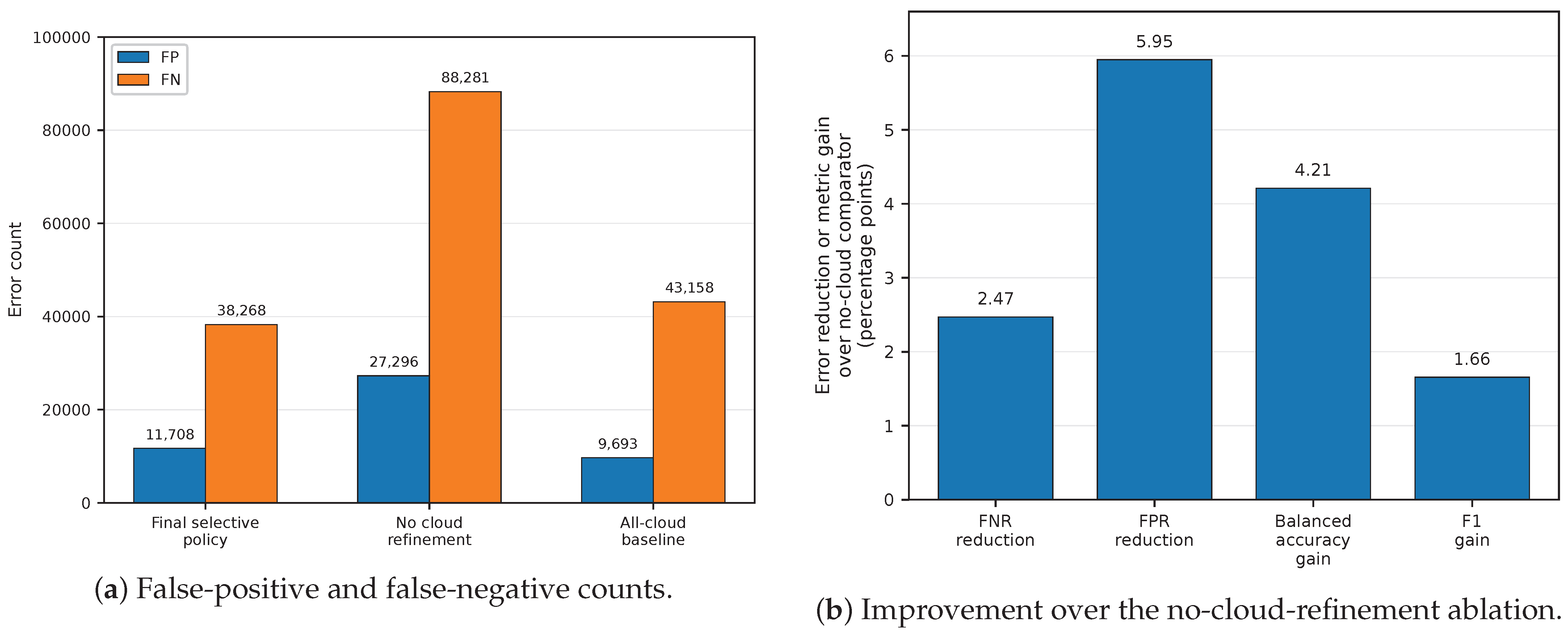
The no-cloud-refinement ablation preserves the principal edge-routing decisions but removes the second-stage classifier for routed flows. FPR increases from $4.47\%$ to $10.42\%$, FNR from $1.89\%$ to $4.36\%$, and balanced accuracy decreases from $96.82\%$ to $92.61\%$. At the selected routing policy, cloud refinement therefore reduces FPR by $5.95$ percentage points and FNR by $2.47$ percentage points, yielding a $4.21$-percentage-point gain in balanced accuracy.

The cloud stage receives all flows shorter than eight packets together with edge-eligible flows that remain unresolved. Its contribution is consequently measured on this selected routed population, not on the flows that satisfy edge-exit conditions. The ablation establishes the value of cloud refinement for routed cases while preserving the route selection imposed by the edge policy.

Figure 10 compares the exact pooled error counts and makes clear that the cloud contribution is evaluated under a fixed route assignment. The all-cloud reference is included only as an operating reference; it does not preserve selective routing or local exits.

5.9. Observation-Budget Sensitivity

Table 19. Sensitivity to the maximum packet-observation budget.

${\mathit{L}}_{\max }$	FP	FN	FPR (%)	FNR (%)	Bal. Acc. (%)	Edge Exits	Edge Share (%)	Mean Exit Packet	Mean Packets Processed
16	12,889	47,581	4.92	2.35	96.36	391,620	17.13	10.94	6.47
32	11,708	38,268	4.47	1.89	96.82	422,190	18.46	12.81	6.93
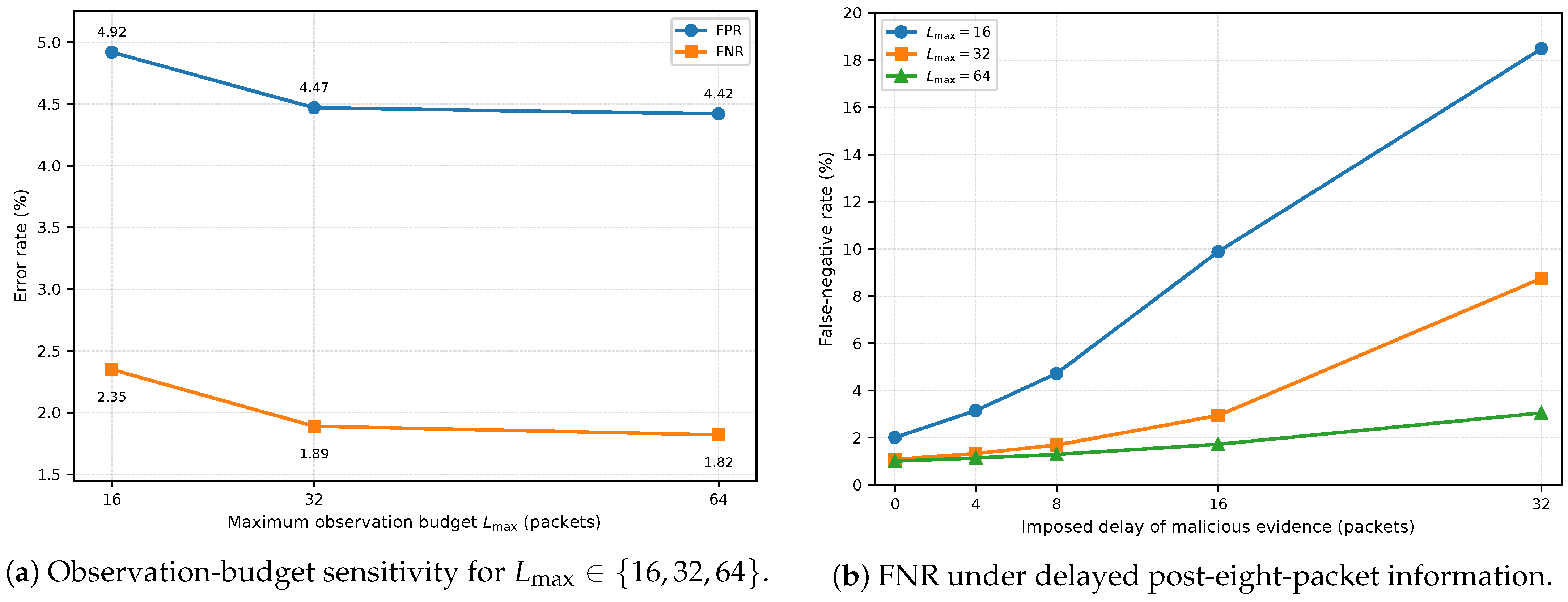
64	11,578	36,851	4.42	1.82	96.88	430,804	18.84	13.37	7.11

compares matched systems with maximum observation budgets of 16, 32, and 64 packets. Increasing the budget from 16 to 32 packets reduces FPR from $4.92\%$ to $4.47\%$, reduces FNR from $2.35\%$ to $1.89\%$, and raises the edge-exit share from $17.13\%$ to $18.46\%$. Extending the budget from 32 to 64 packets yields only a further $0.05$-percentage-point FPR reduction, a $0.07$-percentage-point FNR reduction, and a $0.06$-percentage-point balanced-accuracy gain, while increasing the mean number of processed packets from 6.93 to 7.11. Only $44,820$ flows, or $1.96\%$ of the modeling corpus, reach 64 packets, which limits the population that can benefit from the longer horizon.

The 32-packet setting therefore retains most of the measured gain beyond 16 packets without imposing the longest evaluated horizon. This choice is specific to the observed flow-length distribution and should not be interpreted as a universal early-detection budget.

5.10. Sensitivity to Delayed Post-Eight-Packet Information

The observation-budget comparison preserves the recorded packet sequence.

Table 20. Sensitivity to delayed post-eight-packet information on malicious flows with at least 64 packets.

Delay	${\mathit{L}}_{\max }=16$		${\mathit{L}}_{\max }=32$		${\mathit{L}}_{\max }=64$
(Packets)	FNR (%)	Malicious Edge Exits (%)	FNR (%)	Malicious Edge Exits (%)	FNR (%)	Malicious Edge Exits (%)
0	2.01	65.20	1.08	73.80	1.01	75.60
4	3.15	59.10	1.33	69.60	1.14	73.10
8	4.72	50.40	1.69	62.30	1.29	68.40
16	9.88	31.20	2.94	47.10	1.72	59.20
32	18.48	9.80	8.75	23.40	3.05	42.50

instead delays all post-eight-packet information for the common set of $\mathrm{39,880}$ malicious flows observed through 64 packets, while keeping model parameters, calibration, and thresholds fixed. The resulting changes measure sensitivity to the timing of later prefix information rather than retraining effects; the perturbation does not identify which shifted features are specifically malicious.

With a 16-packet delay, FNR reaches $9.88\%$, $2.94\%$, and $1.72\%$ for $L_{\max }=16$, 32, and 64, respectively. Under a 32-packet delay, the corresponding values are $18.48\%$, $8.75\%$, and $3.05\%$. Malicious edge-exit share declines in parallel. A longer horizon therefore recovers part, but not all, of the displaced post-eight-packet information. The perturbation is a controlled sensitivity test rather than a reconstruction of a specific evasion strategy.

The 32-packet policy is therefore effective when distinguishing behavior appears within the observed prefix, but its recall declines when later prefix information is displaced beyond that horizon. The 64-packet configuration provides partial recovery at a higher observation cost and remains a sensitivity setting rather than the principal policy.

Figure 11 combines the observation-horizon and controlled-delay results. The analysis supports $L_{\max }=32$ as a corpus-specific compromise, not as a universal early-detection horizon, and it shows that delayed post-eight-packet information can limit short-prefix detection in a way that calibration alone cannot remove.

5.11. Deployment-Prior and Alert-Burden Sensitivity

The pooled corpus is attack-dominant, whereas operational IoT traffic may contain a much smaller malicious fraction.

Table 21. Expected alert precision and alert burden under alternative malicious-flow prevalences.

Malicious Prevalence	Policy	Alert Precision (%)	Alerts per ${10}^6$ Flows	False Alerts per ${10}^6$ Flows
10%	Principal static	70.92	138,335	40,225
10%	1% FPR policy	91.46	105,452	9002
10%	0.5% FPR policy	95.49	99,701	4501
1%	Principal static	18.15	54,059	44,248
1%	1% FPR policy	49.34	19,547	9902
1%	0.5% FPR policy	65.79	14,471	4951
0.1%	Principal static	2.15	45,631	44,650
0.1%	1% FPR policy	8.80	10,956	9992
0.1%	0.5% FPR policy	16.01	5948	4996
0.01%	Principal static	0.22	44,788	44,690
0.01%	1% FPR policy	0.96	10,097	10,001
0.01%	0.5% FPR policy	1.87	5096	5000

applies the measured class-conditional error rates to alternative malicious-flow prevalences and reports the resulting alert precision and alert volume per one million flows.

At $1\%$ malicious prevalence, expected alert precision is $18.15\%$ under the principal policy, $49.34\%$ under the $1\%$-FPR policy, and $65.79\%$ under the $0.5\%$-FPR policy. At $0.1\%$ prevalence, the corresponding values are $2.15\%$, $8.80\%$, and $16.01\%$. Thus, even the lower-FPR settings can produce more false than true alerts when attacks are rare. This analysis does not change the measured confusion matrix; it shows how the same class-conditional errors translate into different operational alert burdens as the traffic prior changes.

5.12. Sliding-Window Threshold Updating Under Traffic Drift

Table 22. Static and sliding-window threshold performance in the chronological drift replay.

Policy	FP	FN	FPR (%)	FNR (%)	Bal. Acc. (%)	Edge Share (%)
Static $1\%$-FPR thresholds	4230	1263	1.61	4.34	97.02	15.54
Sliding-window thresholds	2838	1234	1.08	4.24	97.34	15.09

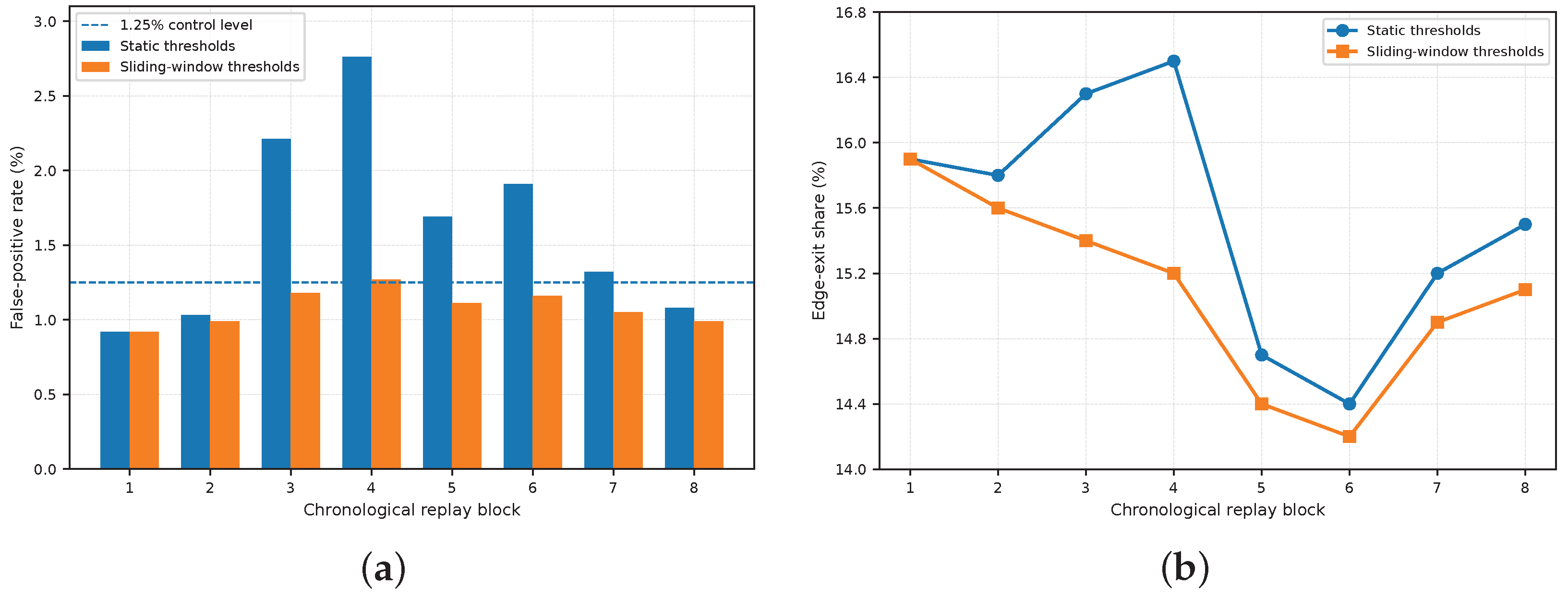
compares the static $1\%$-FPR thresholds with the supervised sliding-window update rule during the chronological drift replay. The replay contains benign-capture changes, attack-mixture changes, and recovery blocks. Under fixed thresholds, the maximum block FPR is $2.76\%$; threshold updating reduces this maximum to $1.27\%$.

Across the complete replay, FPR decreases from $1.61\%$ to $1.08\%$, FNR changes from $4.34\%$ to $4.24\%$, and balanced accuracy increases from $97.02\%$ to $97.34\%$. The edge-exit share decreases from $15.54\%$ to $15.09\%$. Figure 12 shows that adaptation reduces both the magnitude and duration of block-level FPR excursions, with a maximum of $1.27\%$ rather than $2.76\%$. The $1.25\%$ line is an update-control reference, not a deterministic guarantee for every subsequent block. Because the procedure uses delayed adjudicated outcomes, it demonstrates supervised threshold maintenance rather than unsupervised drift detection.

5.13. Policy and Fixed-Checkpoint Comparators

Table 23. Policy and fixed-checkpoint comparators on the pooled PCAP-disjoint evaluation.

Method	FP	FN	FPR (%)	FNR (%)	Bal. Acc. (%)	Edge Share (%)	Cloud Share (%)
All-cloud reference	9693	43,158	3.70	2.13	97.08	0.00	100.00
Fixed checkpoint 8	15,193	45,558	5.80	2.25	95.98	28.26	71.74
Fixed checkpoint 16	13,411	41,510	5.12	2.05	96.42	22.71	77.29
Fixed checkpoint 32	12,181	39,483	4.65	1.95	96.70	4.88	95.12
Sequential principal policy	11,708	38,268	4.47	1.89	96.82	18.46	81.54

compares the sequential policy with an all-cloud reference and fixed decisions at packets 8, 16, and 32. As specified in Section 4.10, each altered route uses a separately fitted, route-matched cloud scaler and classifier. For the fixed-checkpoint policies, flows that do not reach the specified checkpoint are routed to the cloud. The all-cloud reference attains $97.08\%$ balanced accuracy but provides no local exits. The sequential policy attains $96.82\%$ balanced accuracy while resolving $18.46\%$ of all flows at the edge.

The fixed 8-packet policy gives the largest edge share, $28.26\%$, but also the highest FPR, $5.80\%$. Later fixed checkpoints reduce both class-conditional error rates, although fewer flows naturally reach those checkpoints. Relative to the fixed 32-packet policy, the sequential policy increases edge coverage from $4.88\%$ to $18.46\%$ while reducing FPR from $4.65\%$ to $4.47\%$ and FNR from $1.95\%$ to $1.89\%$. Its advantage is therefore a more favorable balance between local coverage and error, rather than uniformly higher accuracy than the all-cloud reference.

5.14. Independent Edge-Model Comparison

Table 24. Matched end-to-end performance of independent causal edge models on the pooled CIC-IoT-2023 evaluation.

Edge Model	FP	FN	FPR (%)	FNR (%)	Bal. Acc. (%)	F1 (%)	Edge Exits	Edge Share (%)
Proposed GRU	11,708	38,268	4.47	1.89	96.82	98.76	422,190	18.46
Lightweight 1D CNN	13,437	45,558	5.13	2.25	96.31	98.53	399,800	17.48
Compact LSTM-attention	11,263	36,851	4.30	1.82	96.94	98.80	414,900	18.14
Temporal convolutional network	12,234	41,712	4.67	2.06	96.63	98.66	406,500	17.78
XGBoost prefix baseline	14,145	48,595	5.40	2.40	96.10	98.44	371,700	16.25

and

Table 25. Edge-model implementation cost measured on a Raspberry Pi 5.

Edge Model	Parameters	Size (KiB)	32-Packet Cost	p50 (ms)	p95 (ms)
Proposed GRU	19,777	77.3	0.58 M	0.31	0.48
Lightweight 1D CNN	18,913	73.9	0.43 M	0.24	0.39
Compact LSTM-attention	29,249	114.3	0.91 M	0.55	0.86
Temporal convolutional network	21,345	83.4	0.62 M	0.29	0.46
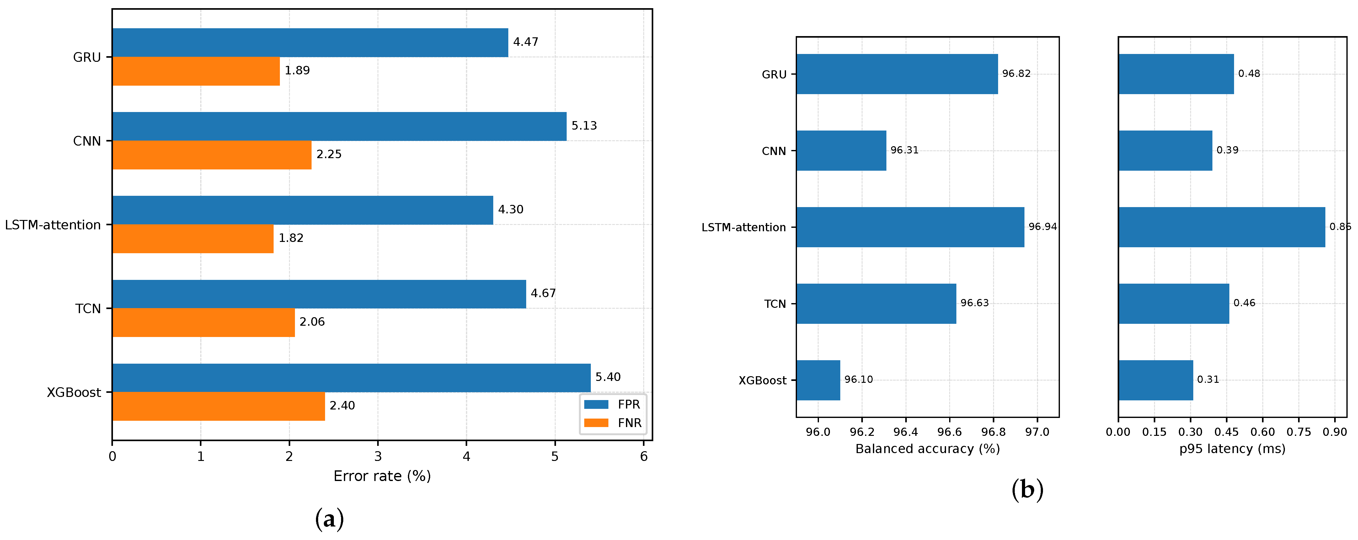
XGBoost prefix baseline	–	1340.0	156 node evaluations	0.19	0.31

jointly compare detection performance and gateway cost. The LSTM-attention model improves balanced accuracy over the GRU by $0.12$ percentage points and reduces FPR and FNR by $0.17$ and $0.07$ percentage points, respectively. This gain is accompanied by a larger model (114.3 versus 77.3 KiB) and higher p95 latency (0.86 versus 0.48 ms). The GRU provides a $0.32$-percentage-point larger edge-exit share. The CNN lowers p95 latency to 0.39 ms but reduces balanced accuracy by $0.51$ percentage points relative to the GRU, while XGBoost gives the lowest latency but the largest serialized model and the weakest balanced accuracy.

No encoder dominates every criterion. Figure 13 summarizes the matched comparison across class-conditional error, balanced accuracy, and gateway latency. The GRU is retained as the principal implementation because it combines near-leading class-conditional error, the largest edge-exit share, compact recurrent state, and moderate single-flow latency.

5.15. CICIDS2017 In-Domain and Cross-Dataset Validation

Table 26. CICIDS2017 in-domain performance on the fixed balanced test set.

Edge Model	FP	FN	FPR (%)	FNR (%)	Bal. Acc. (%)	Edge Share (%)
Proposed GRU	3070	3329	2.85	3.09	97.03	18.00
Lightweight 1D CNN	3490	3739	3.24	3.47	96.64	16.79
Compact LSTM-attention	2930	3135	2.72	2.91	97.18	17.70
Temporal convolutional network	3253	3447	3.02	3.20	96.89	17.20
XGBoost prefix baseline	2747	3997	2.55	3.71	96.87	15.40

reports performance when each model is developed and evaluated within CICIDS2017. The LSTM-attention model attains the highest balanced accuracy, $97.18\%$. The GRU reaches $97.03\%$ balanced accuracy with $2.85\%$ FPR, $3.09\%$ FNR, and an $18.00\%$ edge-exit share, showing that the framework can be developed successfully on the second corpus.

Direct transfer from the single CIC-IoT-2023 transfer-source system fitted for each model family is substantially weaker for every model (

Table 27. Zero-shot transfer from the single CIC-IoT-2023 transfer-source systems to the fixed CICIDS2017 test set.

Edge Model	FP	FN	FPR (%)	FNR (%)	Bal. Acc. (%)	Edge Share (%)
Proposed GRU	12,713	16,807	11.80	15.60	86.30	11.90
Lightweight 1D CNN	14,543	18,637	13.50	17.30	84.60	10.80
Compact LSTM-attention	11,960	16,052	11.10	14.90	87.00	11.50
Temporal convolutional network	13,574	17,129	12.60	15.90	85.75	11.20
XGBoost prefix baseline	17,022	20,575	15.80	19.10	82.55	8.70

). The transfer-source GRU records $11.80\%$ FPR and $15.60\%$ FNR, reducing balanced accuracy to $86.30\%$. The LSTM-attention model transfers slightly better, while XGBoost gives the lowest zero-shot balanced accuracy. PCAP-disjoint validation within CIC-IoT-2023 therefore does not imply invariance to the different traffic and label distribution of CICIDS2017.

Target-calibration-only adaptation recovers part of the lost performance (

Table 28. CICIDS2017 target-calibration-only transfer with frozen CIC-IoT-2023 transfer-source edge models and cloud classifiers.

Edge Model	FP	FN	FPR (%)	FNR (%)	Bal. Acc. (%)	Edge Share (%)
Proposed GRU	6679	11,311	6.20	10.50	91.65	14.60
Lightweight 1D CNN	7648	12,388	7.10	11.50	90.70	13.40
Compact LSTM-attention	6248	10,556	5.80	9.80	92.20	14.20
Temporal convolutional network	7110	11,634	6.60	10.80	91.30	13.90
XGBoost prefix baseline	9588	14,866	8.90	13.80	88.65	11.10

). For the GRU, FPR decreases to $6.20\%$, FNR to $10.50\%$, and balanced accuracy rises to $91.65\%$, while the encoder and cloud-classifier coefficients remain fixed. This recovers $5.35$ of the $10.73$ percentage points lost under zero-shot transfer. The residual gap to the $97.03\%$ in-domain result indicates that score scaling and threshold shift explain only part of the mismatch; representation and conditional-distribution shift remain.

Figure 14 summarizes the three external-validation modes using the exact values in Table 26, Table 27 and Table 28. The target-calibration-only procedure improves both GRU error rates relative to zero-shot transfer, but its FPR and FNR remain above their in-domain values.

5.16. Attack-Family and Attack-Specific Performance

Table 29. Attack-family performance on pooled out-of-fold CIC-IoT-2023 predictions.

Family	Support	FN	FNR (%)	Effective Benign Support	Weighted Reference FP	One-vs.-Benign F1 (%)
DDoS	708,680	7448	1.05	261,955	10,478	98.74
DoS	161,984	2173	1.34	161,984	6803	97.27
Mirai	728,928	8317	1.14	261,955	11,709	98.63
Reconnaissance	303,720	8876	2.92	261,955	13,229	96.39
Spoofing	60,744	2298	3.78	60,744	3159	95.54
Web-based	44,546	5573	12.51	44,546	2517	90.60
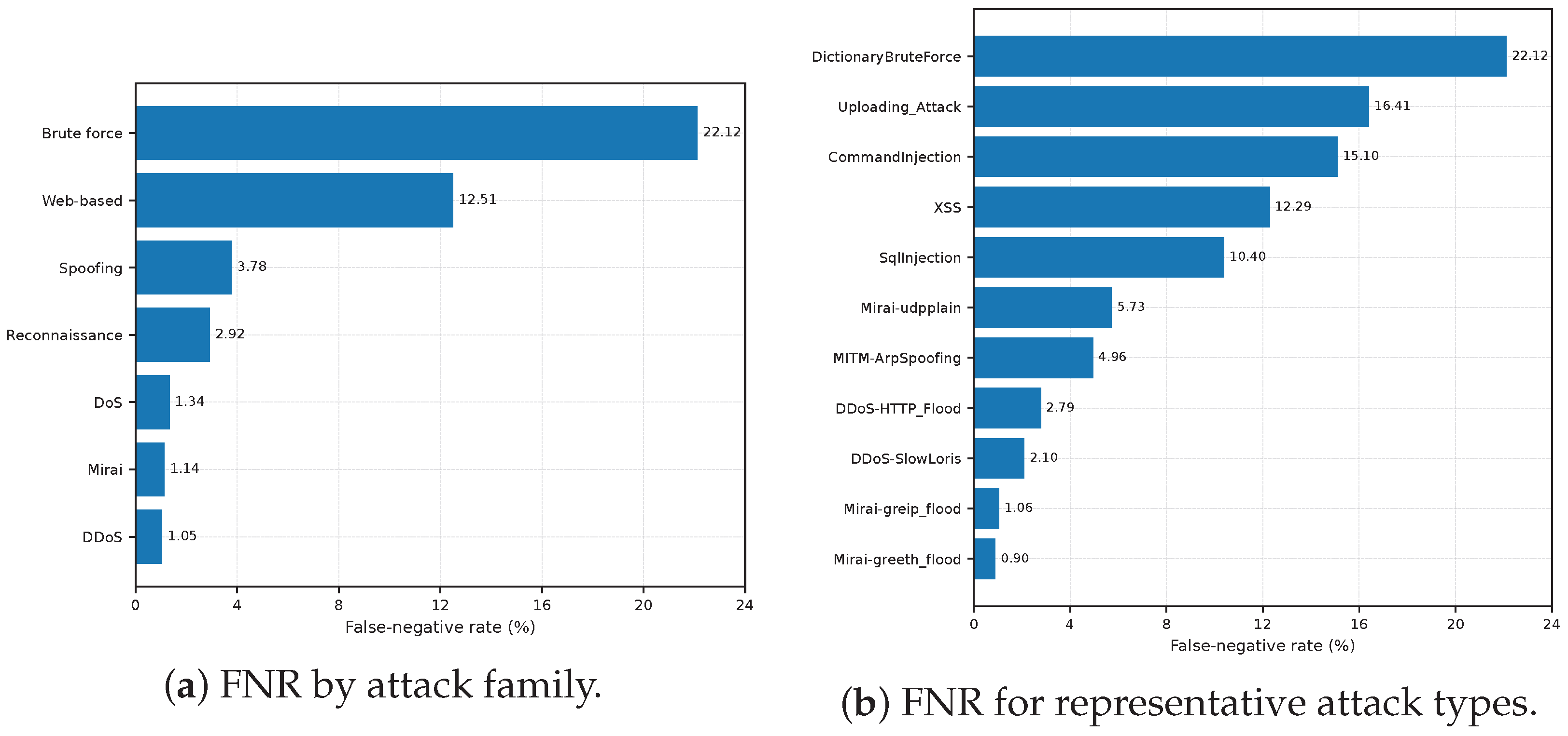
Brute force	16,197	3583	22.12	16,197	1012	84.59

summarizes the pooled results by attack family. The family-level false-negative counts sum to $\mathrm{38,268}$, matching the malicious errors in the principal confusion matrix. DDoS, DoS, and Mirai have FNRs between $1.05\%$ and $1.34\%$. Reconnaissance and spoofing are less reliable at $2.92\%$ and $3.78\%$, while web-based attacks and dictionary brute force reach $12.51\%$ and $22.12\%$, respectively.

Appendix B reports all 33 attack types. Within the DDoS family, DDoS-SYN_Flood has $0.45\%$ FNR, whereas DDoS-SlowLoris and DDoS-HTTP_Flood reach $2.10\%$ and $2.79\%$. The stronger performance on high-rate SYN flooding is consistent with the earlier availability of transport-level evidence, while SlowLoris and HTTP flooding develop more gradually.

Mirai-greeth_flood and Mirai-greip_flood have FNRs of $0.90\%$ and $1.06\%$, but only 282 and 74 flows, respectively, satisfy the eight-packet edge-eligibility requirement. Their performance is therefore driven primarily by end-to-end cloud-routed detection. Mirai-udpplain is more difficult, with $5.73\%$ FNR.

The largest errors occur among reconnaissance, web-based, and brute-force traffic. Recon-PingSweep reaches $6.30\%$ FNR and MITM-ArpSpoofing $4.96\%$. CommandInjection, SqlInjection, Uploading_Attack, and XSS record $15.10\%$, $10.40\%$, $16.41\%$, and $12.29\%$, respectively. DictionaryBruteForce has the highest FNR, $22.12\%$, and the lowest one-vs-benign F1, $84.59\%$. These attack types depend more strongly on evidence that is weakly represented by payload-free packet-prefix features.

Figure 15 summarizes the exact family-level FNRs and representative attack-type values reported in Appendix B. The figure is descriptive of the evaluated scenario-labeled captures; it does not establish exact flow-level attack attribution.

5.17. Contextual Comparison with Recent Lightweight IDS Studies

Table 30. Contextual comparison with recent lightweight edge-oriented IDS studies.

Study	Architecture and Setting	Dataset	Reported Result
Wardana et al. [29]	Hierarchical edge–fog–cloud federated DNN with trust and privacy mechanisms	CIC-IoT-2023 and NF-UNSW-NB15-v2	Accuracy 97.65%; precision 97.65%; recall 100%; F1 98.81%
Nedungadi et al. [30]	LGBM–XGBoost multimodal ensemble deployed on Raspberry Pi 4	Edge-IIoTset	Binary accuracy 98.51%; multiclass accuracy 88.41%; CPU utilization 17–18%
This study	Causal GRU edge exits with selective logistic-regression cloud refinement	309-PCAP CIC-IoT-2023 evaluation	Balanced accuracy 96.82%; FPR 4.47%; FNR 1.89%; edge exits 18.46%

places the present system alongside two recent lightweight edge-oriented IDS studies. Wardana et al. report a hierarchical federated edge–fog–cloud architecture, while Nedungadi et al. report a multimodal ensemble deployed on Raspberry Pi hardware. Their datasets, feature representations, split protocols, objectives, and hardware differ from those used here, so the reported values provide deployment context rather than a controlled performance ranking.

The present study addresses a different combination of requirements: causal packet-prefix inference, calibrated asymmetric exits, an explicit minimum-evidence gate, selective cloud refinement, PCAP-disjoint evaluation, delayed-information sensitivity, low-FPR operation, and separate cross-dataset FPR and FNR. The comparison therefore situates the proposed design within recent lightweight IDS work without treating heterogeneous published results as directly interchangeable.

6. Discussion

The framework occupies an operating region between all-cloud inference and unconditional early classification at the gateway. Selective routing reduces cloud submissions while withholding local decisions for short or unresolved prefixes. Its value, therefore, depends on the joint behavior of observation horizon, class-conditional error, local coverage, gateway cost, and distribution shift rather than on a single aggregate score.

6.1. Observation Horizon and Delayed Information

The maximum observation budget is a deployment parameter rather than an intrinsic property of the framework. In the present corpus, extending the horizon from 16 to 32 packets produces clear improvements in both class-conditional error and edge coverage, whereas the additional gain at 64 packets is small because fewer than $2\%$ of the modeling flows reach that length. The 32-packet setting consequently captures most of the available benefit without extending the principal maximum observation budget to 64 packets.

The delayed-information experiment defines the corresponding boundary of early detection. When post-eight-packet information is displaced beyond the observed prefix, malicious recall and early-exit coverage decline even though the model, calibration, and thresholds remain unchanged. Cloud refinement cannot fully remove this dependence because it also operates on the final available causal prefix rather than on future packets or complete-flow statistics. Longer or adaptive observation may therefore be required for attacks whose identifying behavior develops late, but such policies would exchange earlier decisions for additional evidence.

6.2. False-Positive Control and Threshold Updating

The principal policy gives $4.47\%$ FPR under the selected calibration-risk objective. In benign-dominated deployments, this operating point can generate substantial alert burden even when accuracy and F1 are high. Lower-FPR threshold pairs reduce false alarms by increasing malicious misses and cloud routing; the operating point must therefore reflect the deployment-specific costs of these three outcomes.

The deployment-prior analysis makes this dependence explicit: as malicious prevalence decreases, false alerts dominate the alert stream despite unchanged class-conditional error. The sliding-window experiment addresses a narrower problem. With delayed adjudicated labels, threshold updates stabilize FPR under the evaluated drift sequence while leaving the representation and classifiers fixed. This mechanism supports supervised threshold maintenance, but it cannot correct feature or conditional-distribution shifts that require model adaptation.

6.3. Edge-Gateway Deployment and Lightweighting

The proposed architecture targets gateway-resident inference rather than execution on individual IoT endpoints. The GRU edge model contains $\mathrm{19,777}$ parameters and uses a compact recurrent state, while cloud refinement is implemented by logistic regression over a 97-feature representation. Measurements on a Raspberry Pi 5 show a median 32-packet edge-inference latency of $0.31$ ms and a $0.48$ ms 95th percentile for the GRU implementation. These measurements support the feasibility of single-flow inference on gateway-class hardware, although they do not include packet capture, flow reconstruction, concurrent traffic handling, serialization, or network transfer.

Selective routing reduces the number of representations submitted to the cloud. Under the principal policy, $\mathrm{422,190}$ flows exit locally, reducing the compact feature payload by $18.46\%$, or 156.22 MiB, relative to submitting the same representation for every evaluated flow. The practical saving will depend on transport, encryption, batching, retransmission, and control overhead, which are outside the payload calculation.

The encoder comparison also shows that lightweight deployment does not require a unique model family. The LSTM-attention baseline gives a small accuracy gain at higher parameter and latency cost, whereas the CNN gives lower neural-model latency with weaker detection performance. The GRU provides a balanced streaming implementation, but another causal encoder can be used if it satisfies the same prefix, calibration, and routing constraints. End-to-end gateway latency, energy consumption, sustained packet throughput, and memory pressure under concurrent flows remain to be measured.

6.4. Architectural Trade-Offs and Cross-Dataset Generalization

The matched architecture results separate the routing framework from the edge encoder. Under common causal inputs, calibration, gating, routing, and cloud refinement, the five encoders occupy different error, coverage, storage, and latency operating points. The LSTM-attention model gives the highest balanced accuracy, whereas the CNN and XGBoost favor latency. Encoder selection should therefore follow the gateway’s resource constraints and class-conditional error costs.

The CICIDS2017 experiments distinguish within-corpus validation from cross-dataset transfer. In-domain development remains strong, but the single CIC-IoT-2023 transfer-source system produces substantially higher FPR and FNR under zero-shot transfer. Target-calibration-only adaptation recovers about half of the GRU balanced-accuracy loss, leaving a clear gap to in-domain development. The routing structure is reusable, but deployment on a new traffic domain requires target-representative data and may require model development beyond calibration.

6.5. Attack-Specific Reliability

The family-level and attack-specific results reveal a consistent relationship between available evidence and detection reliability. Flooding attacks generally expose transport-level changes in flags, direction, timing, or packet length within the observed prefix and consequently have low FNR. Web-based attacks and dictionary brute force are more difficult because their distinguishing evidence is more closely associated with application content or later interaction patterns that are excluded from the payload-free causal representation.

The Mirai results illustrate the distinction between end-to-end detection and early edge resolution. Mirai-greeth_flood and Mirai-greip_flood have low FNR, but almost all corresponding flows terminate before the eight-packet gate and are handled by the mandatory cloud route. Their performance therefore reflects successful final classification of short flows rather than frequent early malicious exits. The higher errors for injection, uploading, XSS, and dictionary brute-force traffic identify cases in which richer causal application-layer metadata or a longer selective observation policy may be needed.

These differences are measured under the scenario/file-level labels supplied by CIC-IoT-2023. They characterize variation across the evaluated captures but do not remove possible background or mixed traffic within attack-labeled PCAPs.

6.6. Applicability Across IoT Deployment Domains

The framework is formulated around a gateway-level decision problem rather than the semantics of one application domain. Industrial, smart-city, healthcare, and other multi-device IoT gateways may all observe partial bidirectional flows, face asymmetric costs for benign and malicious decisions, and have access to additional cloud refinement for unresolved traffic. The same routing and calibration structure can therefore be applied wherever these conditions hold.

Application to a new domain nevertheless requires local validation. Traffic prevalence, protocols, device behavior, attack composition, and operational error costs can differ substantially from the evaluated corpora. The deployment-prior analysis shows how strongly alert precision changes under benign-dominated traffic, while the CICIDS2017 experiment shows that a system developed on one corpus does not retain the same error rates under direct transfer. The present evidence supports the framework under PCAP-disjoint validation on CIC-IoT-2023 and after in-domain development on CICIDS2017. The CIC-IoT-2023 summaries pool the four held-out folds and therefore characterize corpus-level out-of-fold performance rather than fold-to-fold stability; fold-specific dispersion and confidence intervals are not reported. Sustained validation on industrial, smart-city, healthcare, and other operational gateway traces remains necessary.

7. Conclusions

This paper presented a reliability-aware edge–cloud framework that treats early IoT intrusion detection as sequential routing over causal flow prefixes. A lightweight GRU, temperature-scaled probabilities, asymmetric exit thresholds, and an eight-packet minimum-evidence gate determine whether a flow exits locally, remains under observation, or receives cloud refinement. Across all 309 CIC-IoT-2023 PCAPs under four outer PCAP-disjoint folds, the 32-packet policy evaluates $\mathrm{2,286,754}$ pooled out-of-fold flows, resolves $18.46\%$ at the edge, and attains $4.47\%$ FPR, $1.89\%$ FNR, $96.82\%$ balanced accuracy, and $98.76\%$ F1 score. Observation-budget and delayed-information analyses identify 32 packets as a corpus-specific compromise and show that late-arriving distinguishing behavior remains a limit of short-prefix detection. Lower-FPR policies and supervised threshold updates provide alternative operating points, while matched encoder comparisons show that no backbone dominates detection quality and gateway cost simultaneously. On CICIDS2017, strong in-domain performance contrasts with weaker zero-shot and target-calibration-only results, demonstrating the need for target-representative development data. The principal limitations remain scenario/file-level CIC-IoT-2023 labels, reduced sensitivity to late or application-dependent attacks, and the absence of sustained measurements of gateway energy, concurrent-flow throughput, and end-to-end processing cost.