Evaluation of Grounding Loss for Very-Low-Frequency Monopole Antennas Based on Tide-Modulated Equivalent Conductivity

Abstract

This paper addresses the challenge of accurately evaluating the grounding loss of coastal very-low-frequency (VLF) monopole antennas under tidal coverage. An equivalent conductivity calculation method based on a layered lossy transmission line model and Wait’s equivalent admittance of ground screens is proposed to obtain the local equivalent conductivity of the tidally covered area. A sector-ring grounding loss model is then established, incorporating tidal depth, coverage area, and ground screen structure, and the effects of tidal coverage extent, tidal depth, non-uniform radial ground screens, and diurnal tidal dynamics on the grounding loss resistance are analyzed. The proposed analytical model is validated against full-wave FEKO simulations over 20–25 kHz, with an average relative error of 6.67%. Results show that when tidal water covers the sparse outer region of the ground screen, the highly conductive seawater layer provides an additional low-resistance return path, reducing grounding loss. When the tide intrudes further into the high-density inner region, current redistribution among the seawater layer, soil, and metallic ground screen weakens the loss reduction or even causes a non-monotonic increase. This work provides a theoretical basis for the tide-adaptive design of grounding systems for coastal VLF antennas.

1. Introduction

The Very low frequency communication systems primarily operate in the 3–30 kHz band. They feature long propagation distances and strong seawater penetration capabilities, making them widely used in long-range ocean communication, deep-sea communication, and subsurface detection [1,2,3,4]. Because the electrical size of a VLF transmitting antenna is much smaller than the operating wavelength, it is generally classified as an electrically small antenna, which exhibits low radiation resistance. Consequently, the loss of the grounding system often becomes the main factor limiting the antenna radiation efficiency. Therefore, a proper evaluation of the grounding loss resistance and its variation is critically important for improving the performance of VLF transmitting systems.

Considerable research has been conducted on grounding systems for VLF antennas. Wait (1973) analyzed the equivalent admittance of a radial ground screen using a transmission-line analogy, laying the foundation for grounding loss calculations. Liu Chao et al. (2008) further developed a method for calculating the grounding loss resistance of VLF umbrella antennas [5,6,7]. Dai Ganlai et al. (2018) analyzed the grounding loss of large VLF umbrella antennas. Li Bin (2019) derived the equivalent admittance of the ground wires of a monopole transmitting antenna and discussed the conductive characteristics of an ideal ground-wire model [8,9,10,11]. Gao Peng et al. (2023) investigated the effect of the ground plane on monopole antenna performance, revealing a nonlinear relationship between ground-screen density and grounding loss [12,13,14]. Furthermore, previous studies on monopole antennas in higher-frequency bands have demonstrated that ground-plane configurations, dielectric loading, and surface-wave effects significantly influence the radiation characteristics [15,16,17,18]. These findings underscore that the electromagnetic coupling between an antenna and its supporting ground environment remains a critical issue across various frequency bands. However, for coastal VLF transmitting antennas, this problem exhibits distinct physical features that differ fundamentally from the aforementioned cases. Specifically, the electrically small dimensions and low radiation resistance of VLF antennas result in grounding-system losses constituting a dominant portion of the total loss. Moreover, the composite conductive structure comprising seawater, soil, and the ground screen, which is formed by tidal inundation, introduces a time-varying nature. Consequently, existing static ground models or microwave monopole models are inadequate for directly describing this scenario. These models are all based on assumptions of an ideal ground plane, a uniform lossy soil, or a static radial ground screen. As a result, they cannot describe the time-varying, non-uniform, and layered conductive characteristics that arise when a coastal area is inundated by tidal water.

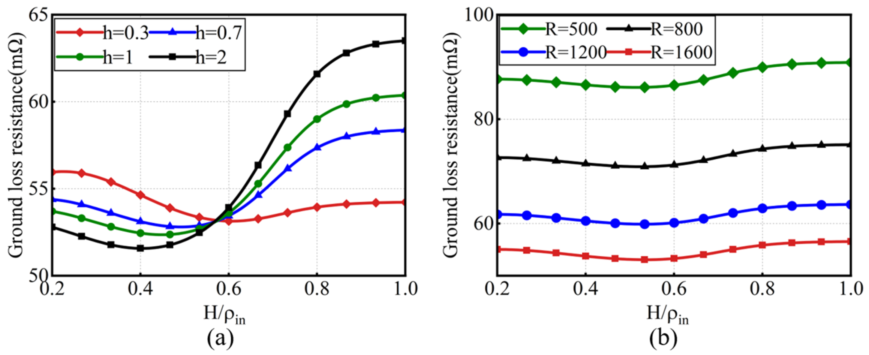
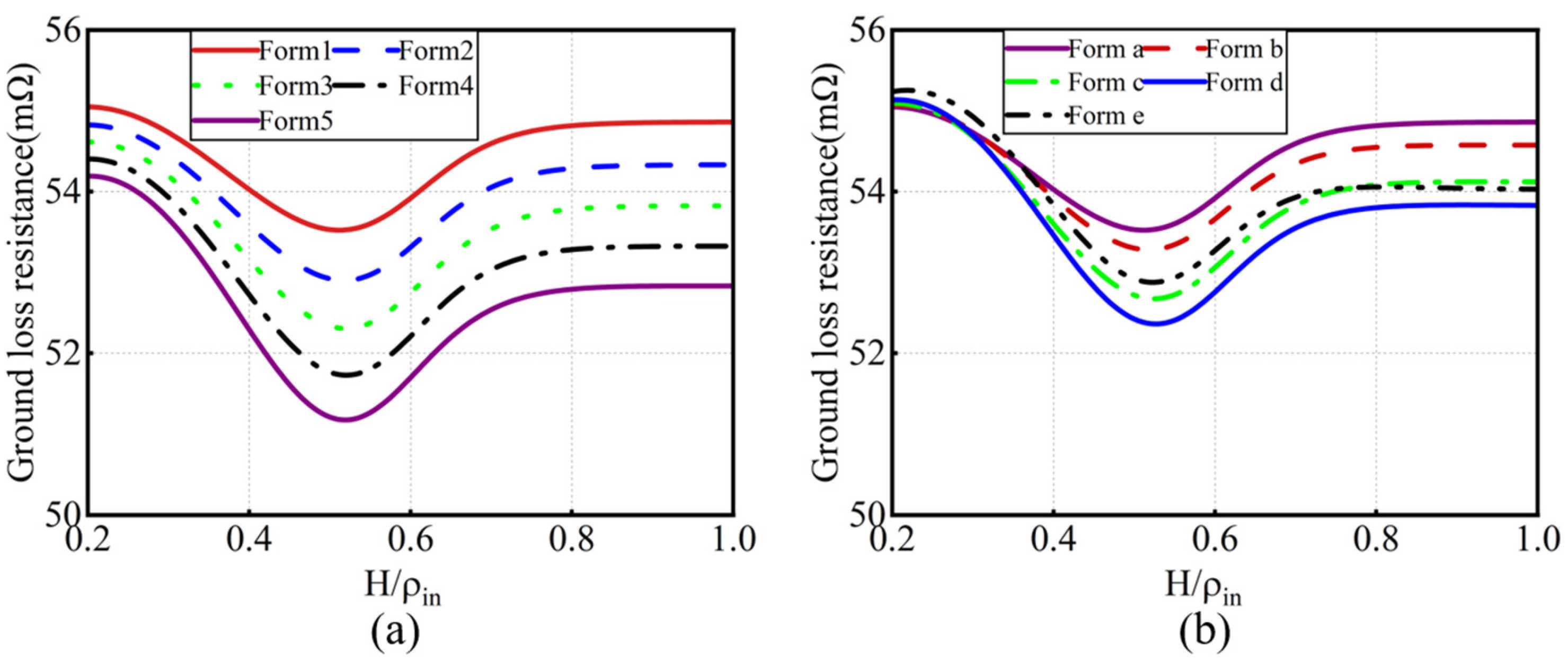
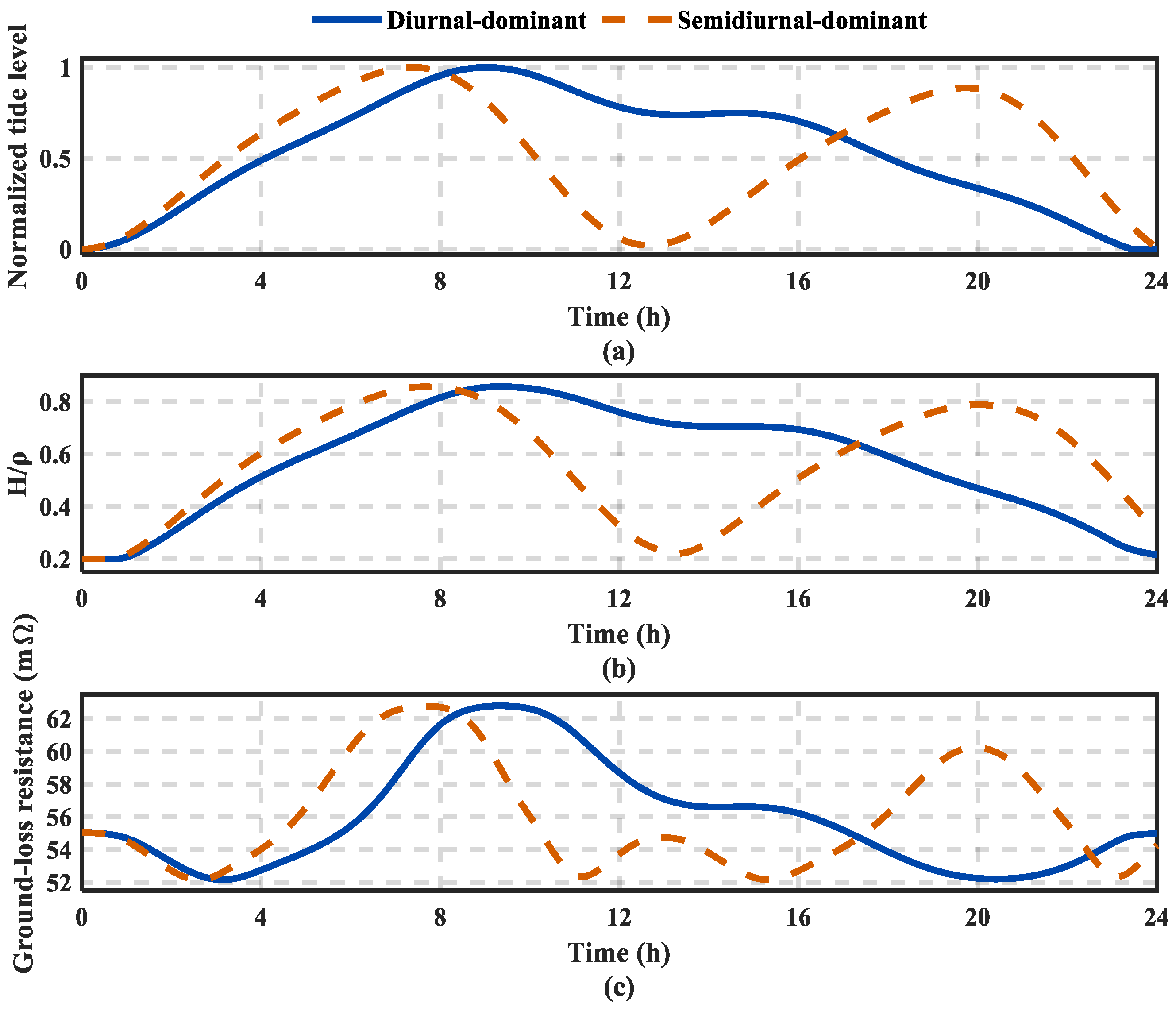
For a coastal VLF transmitting antenna, tidal fluctuations form a composite conductive structure consisting of seawater, soil, and a metallic ground screen. The highly conductive seawater provides a low-resistance return path in the sparsely screened outer region, reducing the grounding loss. However, when the tide intrudes further into the inner region where the ground screen is denser, the skin effect and shielding effect of the finite-depth seawater layer cause a non-monotonic current distribution, and the grounding loss may increase. To address this issue, this paper presents a fast evaluation method for the grounding loss resistance of a VLF monopole antenna under tidal coverage. The tidally covered region is discretized into sector-ring subdomains. Based on a lossy transmission-line model of a finite-depth seawater layer combined with Wait’s equivalent admittance of the ground screen, the local equivalent conductivity is derived. The total grounding loss resistance is then calculated by a weighted integral of the magnetic field in the near field of the monopole. The method is validated by comparative simulations using FEKO (2019) and MATLAB (2023) under different tidal depths, coverage extents, non-uniform ground screens, and dynamic tidal conditions, demonstrating its ability to predict the trend of grounding loss variation under tidal action.

2. Equivalent Calculation Method

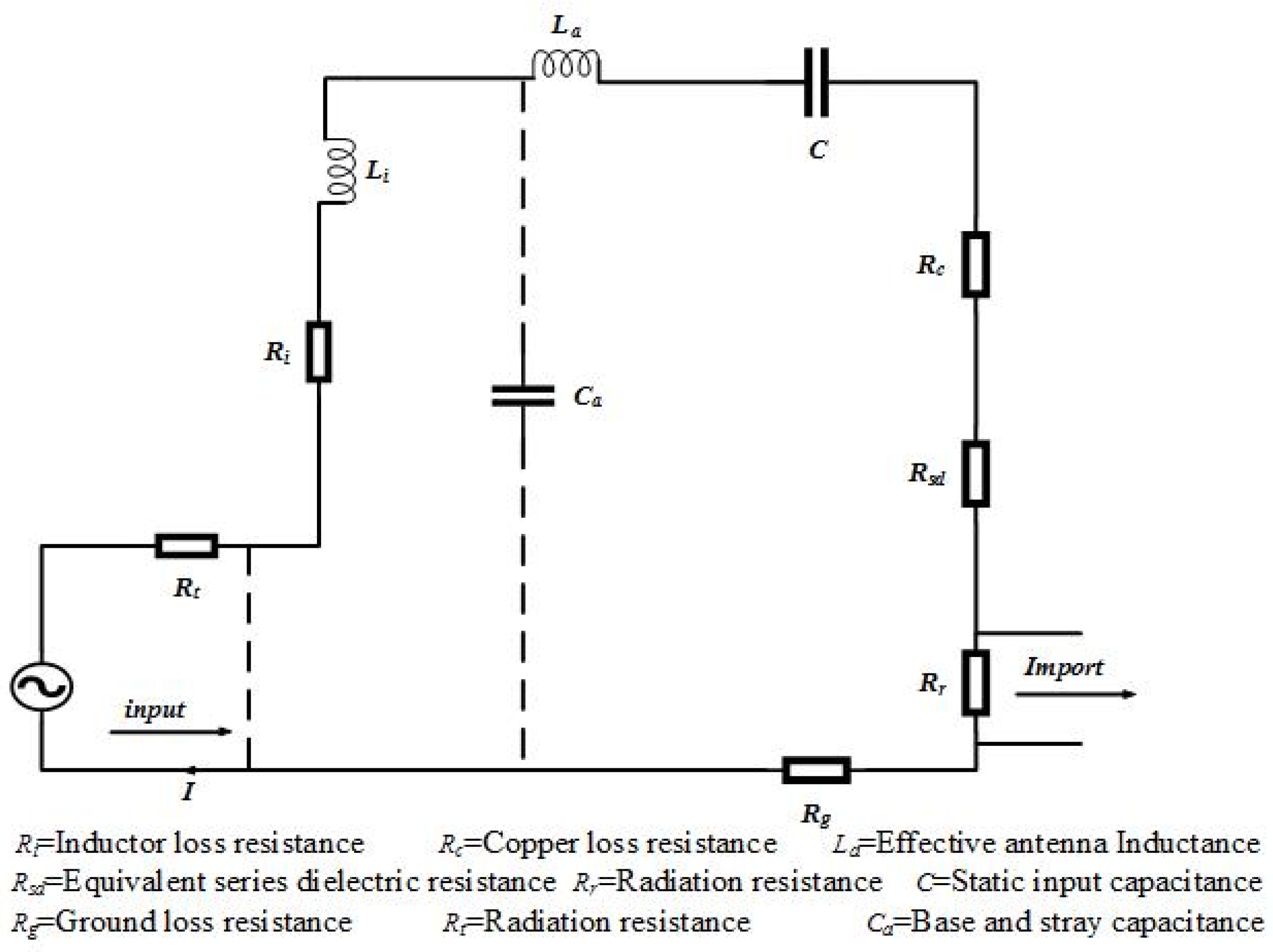
As shown in Figure 1, the equivalent circuit of the VLF transmitting antenna can be characterized by the radiation resistance, grounding loss resistance, and other loss resistances. Among them, hardware-related losses, such as tuning-inductor loss and conductor loss, are usually relatively fixed once the antenna is constructed, whereas the grounding loss resistance varies with the tidal coverage condition. If the radiation resistance, grounding loss resistance, and other loss resistances are denoted by $R_r$, $R_g$, $R_o$, respectively, the radiation efficiency under a given matching condition can be approximately expressed as

$$\eta ={\displaystyle \frac{R_r}{R_r+R_g+R_o}}$$

(1)

Therefore, the tide-induced variation of $R_g$ further affects the radiation efficiency of the antenna. This work focuses on the modeling and analysis of the grounding loss resistance $R_g$ under tidal coverage. The grounding loss mainly consists of two components: the electric-field loss caused by displacement current flowing through the ground into the ground-screen system, and the magnetic-field loss generated by induced currents flowing in the lossy earth layer.

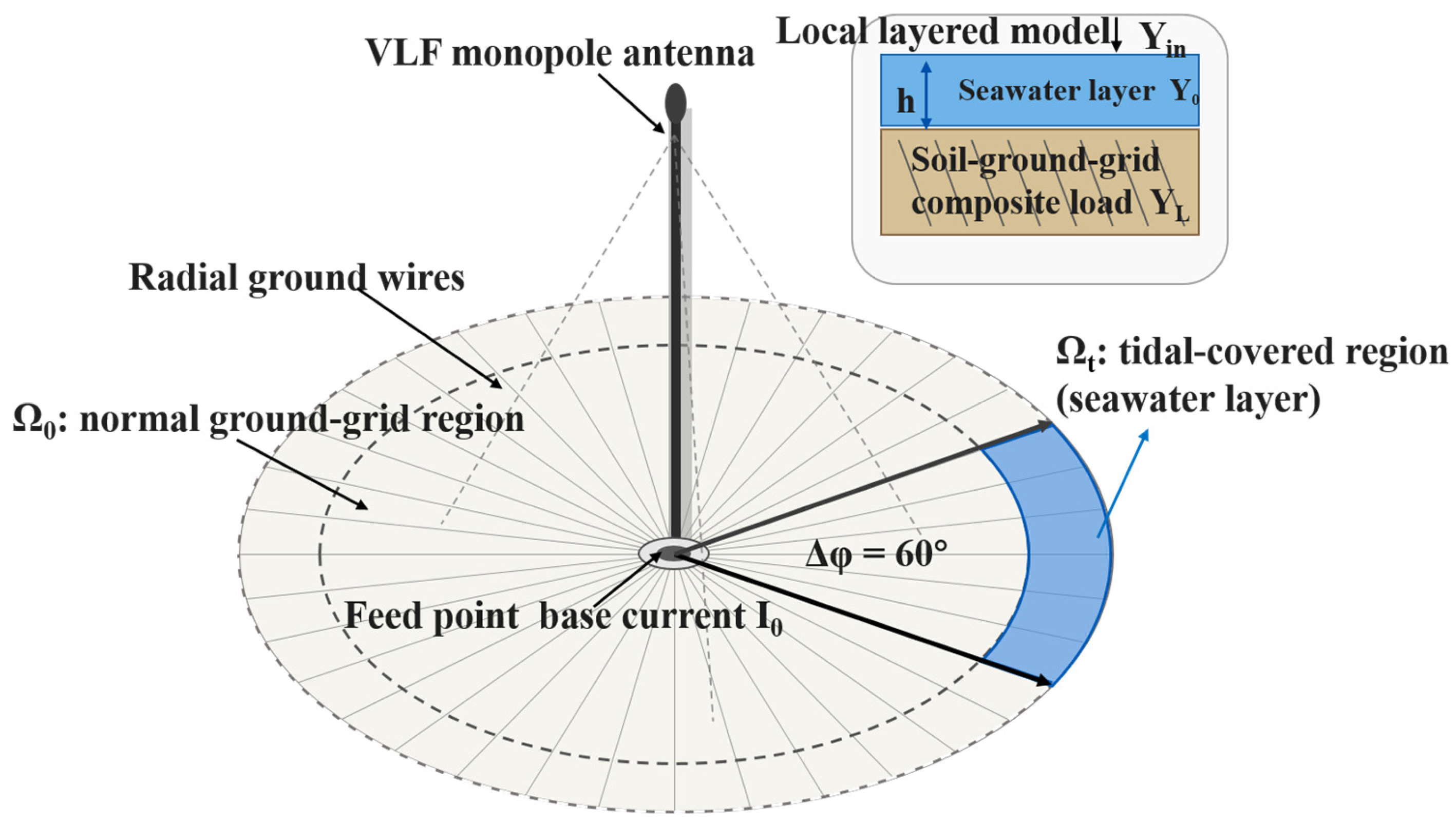
A segmented ground plane model is established as shown in Figure 2, where the light-colored area represents the normal operating area of the ground screen and the blue area represents the tidal coverage area. The effect of the tide on the ground screen is approximated as a sector-shaped region model, constructing the ground plane as a model with a non-uniform conductivity distribution. Based on this, the total grounding loss resistance is solved by deriving the equivalent conductivity and the loss basis per unit area.

To establish a tractable and practically applicable analytical model, appropriate simplifications are introduced for the realistic tidal environment in this study. The primary focus is on the modulation mechanisms of tidal depth, coverage range, and ground-screen configuration on the grounding loss of VLF monopole antennas. Since the tidal water depth is generally much smaller than the horizontal extent of the ground screen, the tidally inundated region is locally approximated as a one-dimensional layered structure. Consequently, a lossy transmission-line model is adopted to characterize the admittance transformation of the finite-thickness seawater layer loaded upon the soil–ground–screen composite structure. Meanwhile, the seawater conductivity, soil conductivity, permittivity, and wire spacing within each sector-ring subregion are assumed to be locally uniform, thereby converting the spatially inhomogeneous problem into a series of regional equivalent conductivity calculations. Furthermore, under VLF conditions, the magnetic field loss induced by return currents in the near-field region dominates the overall loss of the large-scale radial ground screen, whereas the electric field loss is relatively small and is treated as a secondary contribution. Accordingly, this work primarily formulates the model based on magnetic field loss while treating the electric field loss as a secondary term through an approximate consideration. These simplifications substantially reduce the computational burden, enabling a rapid evaluation of how variations in tidal depth, coverage range, and ground-screen layout affect the grounding loss. It should be noted that in realistic coastal environments, factors such as salinity fluctuations, freshwater mixing, seabed sediments, soil moisture content, groundwater distribution, and topographical variations may introduce increased local uncertainty in electromagnetic parameters. These factors primarily influence the calculated results by altering the seawater conductivity, soil conductivity, permittivity, or the boundary of tidal coverage. Therefore, the results presented herein serve as a deterministic baseline prediction for a specified environment. While the aforementioned simplifications do not alter the fundamental physical conclusions regarding the impact of tidal inundation on grounding loss, they may influence the absolute numerical accuracy. For more complex scenarios, further refinement necessitates the integration of in situ measurements, sensitivity analysis, or uncertainty propagation analysis.

According to the literature [1], the characteristic admittance of the soil $Y_s$ is given by

$$Y_s=\sqrt{(\epsilon -{\displaystyle \frac{j\sigma }{\omega }})/\mu }$$

(2)

where $\epsilon$ is the permittivity, $\sigma$ the soil conductivity, $\mu$ the soil permeability, and $\omega$ the angular frequency. For a ground screen system consisting of N radial wires, its characteristic admittance $Y_g$ is defined as:

$$Y_g=1/[jf\mu d_1\ln ({\displaystyle \frac{d_1}{2\pi a}})]$$

(3)

where $d_1=2rsin(\pi /N)\approx 2\pi r/N$ is the distance between adjacent wires, R is the radius of the covered circle, a is the radius of the ground wire, and ω is the frequency. In the non-tidal area, for ease of calculation, the equivalent characteristic admittance of the area without tidal coverage $Y_n$ is defined as:

$$Y_n=\sqrt{\left(\epsilon -{\displaystyle \frac{j{\sigma }_n}{\omega }}\right)/\mu }$$

(4)

where ${\sigma }_n$ is the equivalent conductivity of the area without tidal coverage. Since we are considering the very-low-frequency band, ${\sigma }_n\gg \omega \epsilon$, Equation (3) can be simplified to:

$$Y_n=\sqrt{\left(-{\displaystyle \frac{j{\sigma }_n}{\omega }}\right)/\mu }$$

(5)

According to the conclusion proven by Wait, the ground screen and the soil satisfy the relation $Y_n=Y_s+Y_g$. Then, combining and simplifying the equations yields:

$${\sigma }_n=\sigma +{\displaystyle \frac{2\pi }{Nr\mu \omega \ln \left(\frac{d_1}{2\pi a}\right)}}\sqrt{{\displaystyle \frac{\omega \mu \sigma }{2}}}$$

(6)

The tidal coverage area consists of an upper seawater layer and a lower soil–ground–screen composite structure. The complex conductivity of seawater is defined as ${\tilde{\sigma }}_{sea}={\sigma }_{sea}+j\omega \epsilon$. Calculations show that in the VLF band, the penetration depth of an electromagnetic wave through the seawater layer is on the order of 1–2 m. Since the seawater layer thickness is less than the skin depth in seawater, the electromagnetic field can still partially penetrate the seawater layer and act on the underlying soil–ground–screen composite structure. Therefore, the tidal coverage area cannot be simply equivalent to an infinitely thick seawater layer; the loading effect of the lower soil and ground screen still needs to be considered. The tidal coverage area can be regarded as a layered conductive structure consisting of a finite-thickness seawater layer loaded on top of the soil–ground–screen composite system. Because the tidal depth is much smaller than the horizontal extent of the ground screen, a one-dimensional lossy transmission line model is adopted in the local region to describe the admittance transformation of the seawater layer. The input admittance $Y_{in}$ observed from the upper surface of the seawater layer downward can be expressed as:

$$Y_{in}=Y_0{\displaystyle \frac{Y_L+Y_0\tanh (\gamma h)}{Y_0+Y_L\tanh (\gamma h)}}$$

(7)

where $Y_0$ is the characteristic admittance of the seawater layer, $\gamma$ is the propagation constant in seawater, $h$ is the tidal depth, and $Y_L$ is the load admittance of the soil–ground–screen system. The admittance ratio is defined as $k={\displaystyle \frac{Y_L}{Y_0}}$. For seawater, according to Maxwell’s equations and the wave equations, the propagation constant $\gamma$ is

$$\gamma =\sqrt{j\omega \mu {\tilde{\sigma }}_{sea}}$$

(8)

where ${\tilde{\sigma }}_{sea}$ is the electrical conductivity of seawater. The characteristic admittance of seawater $Y_0$ is

$$Y_0=\sqrt{{\displaystyle \frac{{\tilde{\sigma }}_{sea}}{j\mu \omega }}}$$

(9)

For ease of calculation, $Y_{in}$ is defined as:

$$Y_{in}=\sqrt{{\displaystyle \frac{{\sigma }_e}{j\mu \omega }}}$$

(10)

where ${\sigma }_e$ is the equivalent conductivity in the presence of tidal coverage. The equivalent conductivity of the tidal coverage area ${\sigma }_e$ is then calculated as:

$${\sigma }_e=\mathrm{Re}\left\{j\omega \mu Y_0^2{\left[{\displaystyle \frac{k+\tanh (\gamma h)}{1+k\tanh (\gamma h)}}\right]}^2\right\}$$

(11)

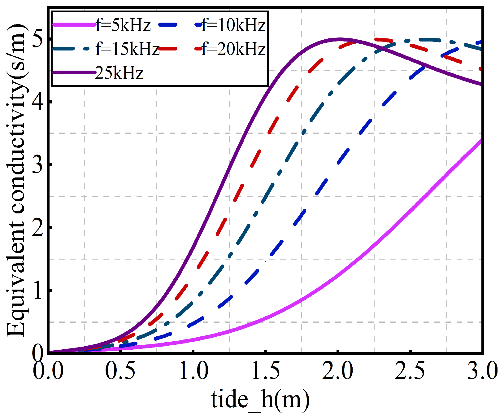
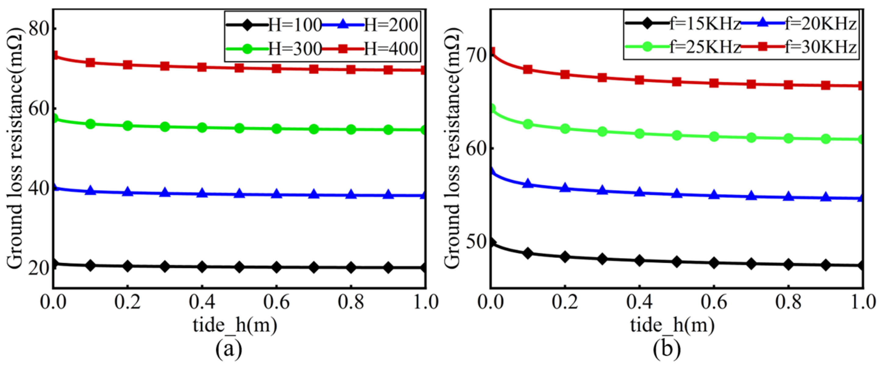
Figure 3 below shows the variation of the equivalent conductivity in the tidal coverage area with tidal depth at different frequencies. Here, in the peripheral region where the ground wires are relatively sparse, the conductivity enhancement effect of the ground screen is weakened. As the tidal depth increases, the highly conductive seawater layer covers the soil surface, causing the equivalent conductivity to increase steadily. When the frequency increases, the skin depth decreases, and the shielding effect of seawater on the ground–screen–soil composite structure becomes stronger; higher frequencies make it easier for this region to reach a seawater-dominated state.

The magnetic field loss resistance per unit area $R_H^{\prime }$, denoted as the base value, is given by [4]:

$$R_H^{\prime }\approx {\displaystyle \frac{2.1\times {10}^{-9}{s}^2{f}^{-1.5}{\sigma }_g^{0.5}{\left(\log \frac{s}{\pi d}\right)}^2}{\left[1+1.06\times {10}^{-6}{s}^{2}f{\sigma }_g{\left(\log \frac{s}{\pi d}\right)}^2+1.45\times {10}^{-3}s{f}^{0.5}{\sigma }_g^{0.5}\log \frac{s}{\pi d}\right]}}$$

(12)

where ${\sigma }_g$ is the equivalent conductivity of the region affected by tidal coverage or of the normally operating ground screen, s is the spacing between buried wires, and d is the wire diameter. For a monopole antenna with a uniform current distribution, the tangential component of the magnetic field $H_{\phi }(\rho )$ in the region where the distance is much smaller than the wavelength is expressed as:

$$H_{\phi }(\rho )={\displaystyle \frac{I_0}{2\pi }}\cdot {\displaystyle \frac{h}{\sqrt{\rho ({\rho }^2+h_{\mathrm{e}}^2)}}}$$

(13)

The vertical electric field $E_{\mathrm{z}}$ is given by

$$E_{\mathrm{z}}={\displaystyle \frac{-I_0}{2\pi j\omega {\epsilon }_0{h}^2}}{[1+{\left(\rho /h_{\mathrm{e}}\right)}^2]}^{-{\displaystyle \frac{3}{2}}}$$

(14)

where $\rho$ is the distance from the base of the monopole antenna, $h_{\mathrm{e}}$ is the effective height, ${\epsilon }_0$ is the relative permittivity, and $I_0$ is the base current. According to the method based on the magnetic field loss resistance per unit area, the magnetic field loss resistance $R_H$ is

$$R_H={{\displaystyle \int }}_{{\mathsf{\Omega }}_g}{R}_H^{\prime }{\left|{\displaystyle \frac{H_{\phi }(\rho )}{I_0}}\right|}^{2}dS$$

(15)

In polar coordinates, the magnetic field weighting function $W_H$ is defined as:

$$W_H={\left|{\displaystyle \frac{H_{\phi }(\rho )}{I_0}}\right|}^2\rho$$

(16)

Under non-tidal conditions, the reference magnetic field loss resistance $R_{H0}$ is

$$R_{H0}=2\pi {\int }_0^{R_g}{R}_{H0}^{\prime }{W}_{H}d\rho$$

(17)

where $R_g$ is the coverage radius of the ground screen. The contribution of the tidal coverage area to the total magnetic field loss under non-tidal conditions $R_{H0}^t$ is

$$R_{H0}^t={\theta }_t{\int }_{r_{\mathrm{in}}}^{r_{\mathrm{out}}}{R}_{H0}^{\prime }{W}_{H}d\rho r_{out}$$

(18)

where $r_{in}$ and $r_{out}$ are the inner and outer boundaries of the tidal coverage area, respectively, and ${\theta }_t$ is the tidal coverage angle. The tidal coverage location influence factor ${\eta }_p$ is defined as:

$${\eta }_p={\displaystyle \frac{R_{H0}^t}{R_{H0}}}.$$

(19)

Substituting Equations (16) and (17) into Equation (18) yields

$${\eta }_p={\displaystyle \frac{{\theta }_t{\int }_{r_{in}}^{r_{out}}{R}_{H0}^{\prime }{W}_{H}d\rho }{2\pi {\int }_0^{R_g}{R}_{H0}^{\prime }{W}_{H}d\rho }}$$

(20)

When the tidal depth is h, the magnetic field loss in the tidal coverage area $R_{Ht}^t(h)$ is

$$R_{Ht}^t(h)={\theta }_t{\int }_{r_{in}}^{r_{out}}{R}_{Ht}^{\prime }{W}_{H}d\rho$$

(21)

The tidal depth influence factor ${\eta }_h$ is defined as:

$${\eta }_h={\displaystyle \frac{R_{Ht}^t(h)}{R_{H0}^t}}$$

(22)

Substituting Equations (20) and (17) into Equation (21) gives

$${\eta }_h={\displaystyle \frac{{\int }_{r_{\mathrm{in}}}^{r_{\mathrm{out}}}{R}_{Ht}^{\prime }{W}_{H}d\rho }{{\int }_{r_{\mathrm{in}}}^{r_{\mathrm{out}}}{R}_{H0}^{\prime }{W}_{H}d\rho }}$$

(23)

After tidal coverage, the non-tidal region still uses $R_{H0}^{\prime }$, while the tidal coverage region uses $R_{Ht}^{\prime }$. The total magnetic field loss resistance $R_m$ is then

$$R_m={{\displaystyle \int }}_{{\mathsf{\Omega }}_0}{R}_{H0}^{\prime }{W}_{H}d\rho d\varphi +{{\displaystyle \int }}_{{\mathsf{\Omega }}_t}{R}_{Ht}^{\prime }{W}_{H}d\rho d\varphi$$

(24)

where ${\mathsf{\Omega }}_0$ is the non-tidal area and ${\mathsf{\Omega }}_t$ is the tidal coverage area. Using Equations (19) and (22), the total magnetic field loss resistance in Equation (23) can be simplified to

$$R_m=R_{H0}\left[1+{\eta }_p\left({\eta }_h-1\right)\right].$$

(25)

The electric field loss resistance $R_E$ is given by

$$R_E={\displaystyle \frac{1}{I_0^2}}{\int }_{A1}{R}_{E_1}^{\prime }{J}_z^{2}d{A}_1+{\int }_{A_2}{R}_{E2}^{\prime }{J}_z^{2}d{A}_2$$

(26)

where $J_{z }=\omega {\epsilon }_{0 }{E}_z$ is the conduction current density and $R_{E_1}^{\prime }$, $R_{E2}^{\prime }$ is the electric field loss per unit area in the normal region and the tidal coverage region, respectively. $A_1=\pi R^2-A_2$, $A_2={\displaystyle \frac{1}{2}}(R-D{)}^2\theta$ where R is the ground screen radius in the coverage area and D is the radius of the inner circular normal ground screen region. In the VLF band, for a large-scale radial ground screen system, magnetic field loss usually dominates. Therefore, the total loss resistance $R_g$ can be approximated as:

$$R_g\simeq R_{H0}\left[1+{\eta }_p\left({\eta }_h-1\right)\right]$$

(27)

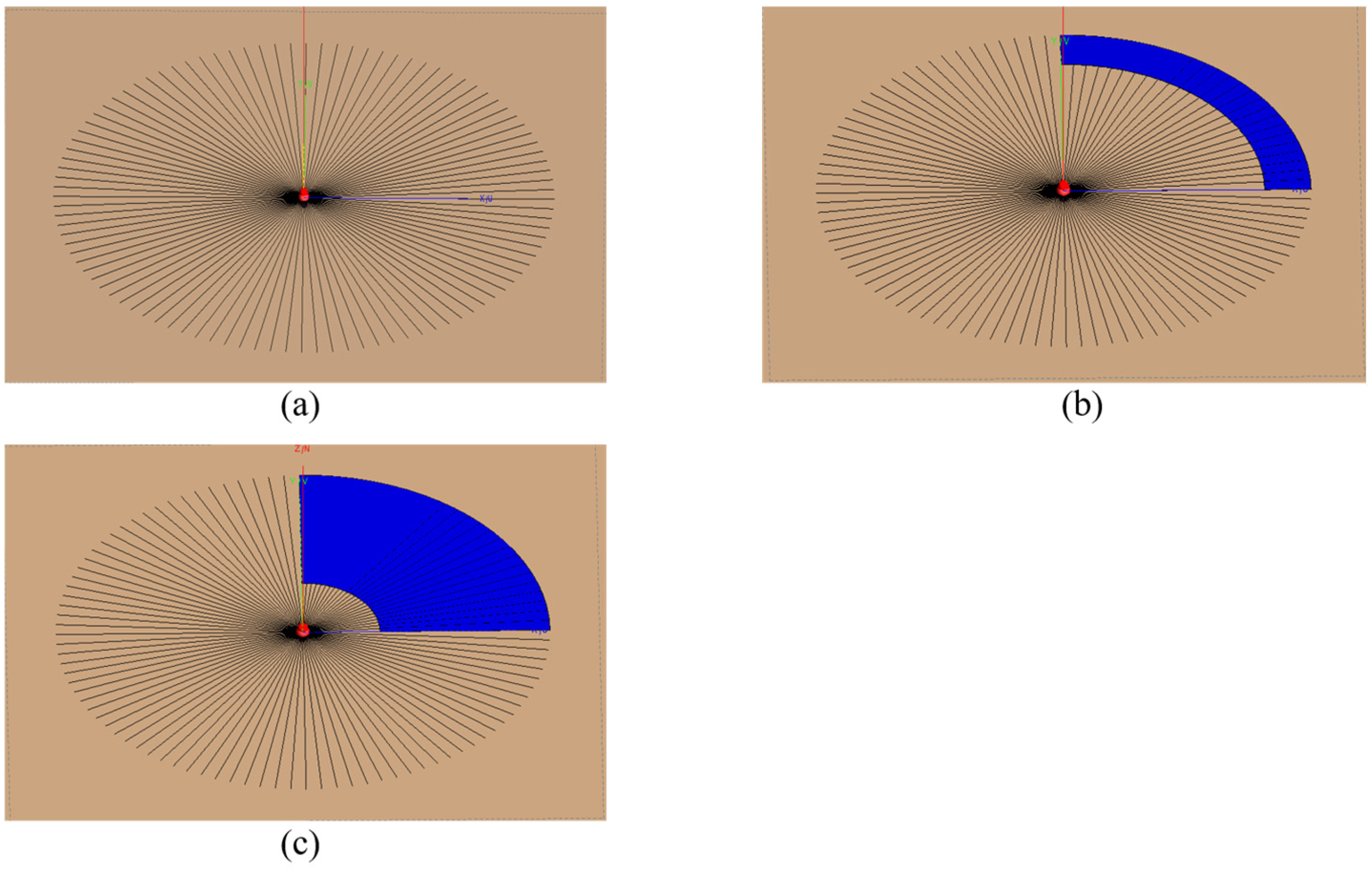
To validate the effectiveness of the proposed method for calculating the grounding loss resistance under tidal coverage, the model results are compared with full-wave simulations performed using FEKO. Figure 4 shows the tidal simulation model established in FEKO The monopole antenna height is set to 300 m, and its ground screen system consists of 100 radial ground wires with an angular spacing of 3.6°. The coverage radius of the ground screen system is 1600 m. The tidal coverage area is set to an azimuthal angle of 60° and is located in the outer annular region from 1300 m to 1600 m. The blue area in the figure indicates the tidal coverage region. The tidal depth is 0.5 m. The ground conductivity is set to 0.01 S/m, and the seawater conductivity is set to 4 S/m.

Table 1. Comparison of grounding loss resistance results.

Frequency/kHz	Analytical Total Loss/mΩ	Simulated Loss/mΩ	Loss Under Non-Tidal Condition/mΩ
20	55.05	51.88	57.57
21	56.90	53.51	59.52
22	58.71	55.09	61.44
23	60.51	56.72	63.33
24	62.26	58.20	65.18
25	63.99	59.64	67.01

presents a comparison between the proposed analytical model and the FEKO simulation results. It can be observed that in the 20–25 kHz frequency band, the grounding loss resistance obtained by both methods increases with frequency, and the loss under non-tidal conditions is always greater than that under tidal conditions. Taking 20 kHz as an example, the grounding loss resistance calculated by the analytical model is 55.05 mΩ, while the FEKO simulation yields 51.88 mΩ, with a relative error of approximately 5.76%. The FEKO result is slightly lower than the analytical value, mainly due to the coupling effects between the seawater layer, the ground screen wires, and the finite region boundaries, as well as the mesh discretization issues inherent in the full-wave model. Overall, the grounding loss resistances from the two methods show good consistency in terms of frequency trend and the loss reduction behavior induced by tides. The loss reduction in this model is mainly attributed to the highly conductive seawater layer effectively shunting the current that would otherwise flow through the soil, thereby reducing the loss. Although the improvement appears modest, this is because the tidal area is located at the outermost edge of the ground screen, where the current density has already decayed significantly, limiting its contribution to the total loss.

Table 2. Comparison of accuracy consistency and computational characteristics between the proposed method and FEKO simulation.

Method	Main Procedure	Computational Scaling	Typical Execution Time
Proposed analytical method	Equivalent conductivity + weighted integration	Increases approximately linearly with the number of subregions and frequency points	Approximately 5–15 s.
FEKO full-wave simulation	3D modeling + meshing + field solving	Depends on mesh unknowns and solver settings	Approximately 20–60 min.

further presents a comparative analysis of the computational characteristics between the proposed method and the FEKO full-wave simulation. Combined with Table 1, it can be observed that the proposed method demonstrates good agreement with the FEKO results while substantially reducing the typical computation time from the minute scale to the second scale. Therefore, this method is better adapted for fast parametric evaluations across diverse tidal depths, coverage ranges, frequencies, and ground-screen structures, whereas FEKO is well suited as a high-precision verification approach for representative operating scenarios.

3. Simulation Validation

3.1. Grounding Loss Resistance for Different Tidal Depths

Figure 5 presents the variation of grounding loss resistance with tidal depth under outer-rim tidal coverage. Because the tidally covered region is located at the outer periphery of the ground screen, where the wire spacing is relatively large and the inherent current-carrying capacity is weak, the seawater layer provides an additional conductive path in this peripheral region as the tidal depth increases, thereby increasing the local equivalent admittance. Consequently, the grounding loss resistance exhibits an overall decreasing trend. From Figure 5a, it can be seen that the curves follow the same trend for different monopole antenna heights, but the loss values and the magnitudes of reduction differ, indicating that the near-field distribution of the antenna affects the contribution of the tidally covered region to the total loss. As shown in Figure 5b, the loss resistance decreases with increasing tidal depth at all frequencies, and the strength of the coupling between the seawater layer and the underlying ground–screen–soil composite structure varies with frequency, which leads to differences among the curves at different frequencies.

3.2. Grounding Loss Resistance for Different Tidal Coverage Areas

Figure 6 illustrates the variation of grounding loss resistance under different tidal coverage areas. As shown in Figure 6a, as the tidally covered region gradually expands from the outer periphery of the ground screen inward toward the inner area, the loss resistance first decreases and then increases. In the peripheral region, the loss resistance generally decreases with increasing tidal depth. However, when the coverage extends further into the inner area, the loss resistance rises to some extent, and this trend becomes more pronounced at larger seawater depths. From Figure 6b, it can be observed that, similar to previous findings, increasing the ground screen radius also significantly reduces the grounding loss resistance under the same tidal coverage conditions. The curves for different ground screen radii exhibit a generally similar trend: when the ground screen radius is small, the loss resistance is relatively high, and as the radius increases, the loss resistance gradually decreases. Overall, the location of tidal coverage has a significant impact on the grounding loss, and the magnitude of variation in the loss resistance also changes with increasing tidal depth and ground screen radius.

3.3. Grounding Loss Resistance for Non-Uniform Radial Ground Screen Distribution

To accurately analyze the influence of a non-uniform radial ground wire network on grounding loss under tidal effects, the ground wire coverage area is radially divided into three zones: 0–500 m (inner zone with the highest current density), 500–1000 m (middle zone with moderate current density), and 1000–1600 m (outer zone with the lowest current density and the sparsest ground wires).

Table 3. Ground screen distributions under different configurations.

No	Number of Wires in the First Segment (0–500 m)	Number of Wires in the Second Segment (500–1000 m)	Number of Wires in the Third Segment (1000–1600 m)
1	100	100	100
2	120	110	90
3	140	120	80
4	160	130	70
5	180	140	60

presents five allocation schemes (1–5) with different radial wire counts, and

Table 4. Non-uniform ground screen distributions under equal copper consumption.

No	Number of Wires in the First Segment (0–500 m)	Number of Wires in the Second Segment (500–1000 m)	Number of Wires in the Third Segment (1000–1600 m)
a	100	100	100
b	120	92	90
c	140	84	80
d	160	76	70
e	180	68	60

provides five equal-copper-quantity non-uniform distribution schemes (a–e) under the constraint of a constant total copper wire length, enabling a comparative study of the modulation effect of ground wire density redistribution on grounding loss.

Figure 7 illustrates the modulation of grounding loss resistance by non-uniform radial ground screen configurations under tidal intrusion. Overall, the two sets of results exhibit similar trends to those obtained in previous sections regarding the effect of the coverage area. When the tide primarily covers the outer periphery, the loss resistance decreases as the tidal intrusion range expands. However, when the tide further extends into the near region, the loss reduction trend weakens and even increases slightly. Figure 7a shows the case of non-equal copper consumption. As the wires gradually concentrate toward the inner and middle regions, the total wire length increases, leading to a reduction in the overall grounding loss resistance. This indicates that increasing the ground screen density in the main return-current region can effectively reduce the equivalent grounding loss. Figure 7b presents the equal copper consumption configuration. The differences among the curves are relatively small, suggesting that when the total wire length is constrained, the improvement achieved by radial redistribution is limited. It is worth noting that simply increasing the wire density in the inner region does not necessarily yield the best performance over the entire tidal intrusion range. If the ground screen in the outer and middle regions becomes excessively sparse, the current-carrying capacity during the outer-periphery tidal coverage stage is compromised. In comparison, an optimal non-uniform ground screen design should not rely solely on increasing the wire density in the near region; instead, it should comprehensively consider the coupling relationships among the tidal coverage location, the weighting of the return current, and the radial distribution of the ground screen. Consequently, the radial configuration of the ground screen should not be designed solely based on minimizing the grounding loss under tideless conditions; the stability of the grounding loss throughout the tidal cycle must also be taken into consideration. For coastal VLF antennas, the design process should first identify the frequently inundated areas according to site-specific tidal statistics, and subsequently determine the radial wire allocation by incorporating the weighting of the near-field magnetic field. Specifically, if the tidal effect is predominantly confined to the outer periphery, sufficient conductive continuity must be ensured in the outer and middle regions to utilize the low-resistance return path formed by the seawater layer. Conversely, if the tide is likely to penetrate further into the near-field region, an excessively non-uniform ground screen distribution should be avoided to prevent pronounced current redistribution induced by the tidal inundation. Therefore, a more rational design objective is not merely to minimize the grounding loss under a single operating scenario, but rather to attain a comparatively low and stable grounding loss with limited fluctuation over a typical tidal cycle. To provide a compact quantitative comparison among different ground–screen layouts, a tide-weighted grounding loss metric is introduced following reference [19]:

$$W_T=R_T\cdot C_L={\displaystyle \frac{R_m}{R_f}}\cdot {\displaystyle \frac{L}{L_f}}$$

(28)

where $R_T$ is the normalized tidal grounding loss term and $C_L$ is the normalized wire-consumption term. $R_m$ is the root-mean-square value of the grounding loss resistance over a representative tidal process, given by

$$R_m=\sqrt{{\displaystyle \frac{1}{N}}{\displaystyle \sum _{k=1}^N}{R}_g^2(k)}.$$

(29)

Here, R_g(k) denotes the grounding loss resistance at the kth sampled tidal state and N is the total number of sampled tidal states. R_f and L_f denote the root-mean-square grounding loss resistance and total wire length of the reference ground–screen configuration under the same tidal process, respectively, while $L$ is the total wire length of the current configuration. A smaller $W_T$ indicates a better trade-off between reduced grounding loss and lower wire consumption. For equal-copper configurations, $C_L=1$, and the metric reduces to the normalized tidal grounding loss level.

3.4. Simulation of the Temporal Evolution of Grounding Loss Resistance Under Diurnal Tidal Dynamics

Figure 8 illustrates the diurnal variations of tidal level, tidal inundation range, and ground loss resistance under diurnal tide and semi-diurnal tide conditions over a 24 h period. Under a diurnal-tide-dominant scenario, the tidal level exhibits one rise and one fall; under a semi-diurnal-tide-dominant scenario, two rises and two falls occur within 24 h. Correspondingly, the tidal inundation range in Figure 8b expands and retreats synchronously with the tidal level. As shown in Figure 8c, the ground loss resistance also exhibits periodic variations driven by the tide. When the tide advances from the outer periphery inward, the loss resistance tends to decrease; however, when the tide further propagates into the inner region where the water depth becomes significant, the loss resistance increases. In the semi-diurnal tide case, two loss fluctuations are observed within one day, but their amplitudes are not equal, indicating that the tidal type determines the characteristics of the ground loss variation. Furthermore, under different tidal models, the occurrence times of the maximum and minimum loss resistances differ, and the antenna radiation efficiency fluctuates accordingly with the tide. For the tidal parameters adopted in this simulation, the loss resistance is relatively high from morning to noon, resulting in lower radiation efficiency, while the opposite trend occurs at night. It should be noted that in practice, the tidal phase shifts backward by approximately one hour per day, so the occurrence times of the extreme loss values also shifts day by day.

4. Conclusions

In this paper, an evaluation model for the grounding loss resistance of a VLF monopole antenna under tidal coverage is established, and the effects of tidal depth, coverage location, ground screen configuration, and diurnal tidal variation on the grounding loss are analyzed. It is found that the grounding loss under tidal action exhibits spatial dependence and non-monotonic behavior. When the tide covers the sparse outer periphery of the ground screen, the highly conductive seawater layer provides an additional low-resistance return path for the return current, thereby reducing the grounding loss. When the tide further extends into the inner region where the ground screen density is higher, the current is redistributed among the seawater layer, the soil, and the metallic ground screen, and the current-carrying capacity of the metallic ground screen diminishes; consequently, the loss reduction trend weakens and even reverses to an increase. In non-uniform ground screen designs, appropriately increasing the wire density in the inner region while maintaining sufficient conductivity in the outer region can mitigate the adverse effects of tides. Furthermore, the diurnal tidal dynamic analysis indicates that the grounding loss resistance fluctuates with the tidal cycle in an asymmetric bimodal or unimodal pattern, reflecting the time-shift regulation of antenna performance by the tidal phase. The proposed method provides a reference for the tide-adaptive design of grounding systems for coastal VLF antennas.