Author Contributions
Conceptualization, Y.L., J.Z. and K.X.; methodology, J.Z. and K.X.; software, J.Z.; validation, Y.L., J.Z., Y.Z. and M.Y.; formal analysis, J.Z.; investigation, Y.L., Y.Z. and M.Y.; resources, K.X. and J.-B.H.; data curation, Y.L., J.Z., Y.Z. and M.Y.; writing—original draft preparation, J.Z.; writing—review and editing, Y.L., J.Z., Y.Z., M.Y., K.X. and J.-B.H.; visualization, J.Z.; supervision, K.X. and J.-B.H.; project administration, K.X.; funding acquisition, K.X. All authors have read and agreed to the published version of the manuscript.
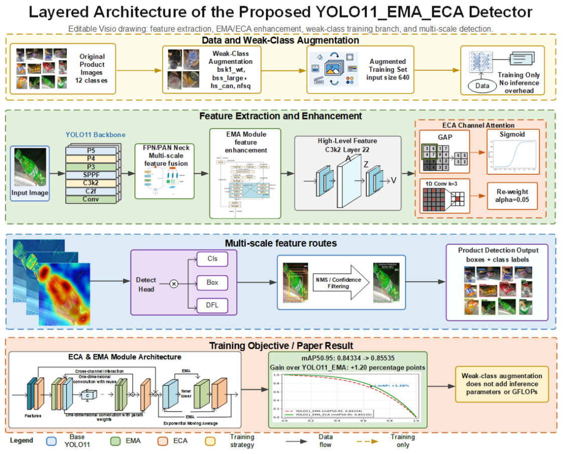
Figure 1.
Overall architecture of the proposed WCA-Det framework. Weak-class augmentation is used only during training, whereas the EMA and ECA components enhance feature representation inside the detector. Arrows indicate data flow, and dashed boxes separate data preparation, feature enhancement, detection, and result-summary stages.
Figure 1.
Overall architecture of the proposed WCA-Det framework. Weak-class augmentation is used only during training, whereas the EMA and ECA components enhance feature representation inside the detector. Arrows indicate data flow, and dashed boxes separate data preparation, feature enhancement, detection, and result-summary stages.
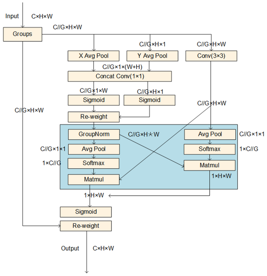
Figure 2.
Structure of the EMA multi-scale feature enhancement module, showing feature grouping, cross-spatial interaction, and re-weighting. The asterisk (*) denotes element-wise multiplication.
Figure 2.
Structure of the EMA multi-scale feature enhancement module, showing feature grouping, cross-spatial interaction, and re-weighting. The asterisk (*) denotes element-wise multiplication.
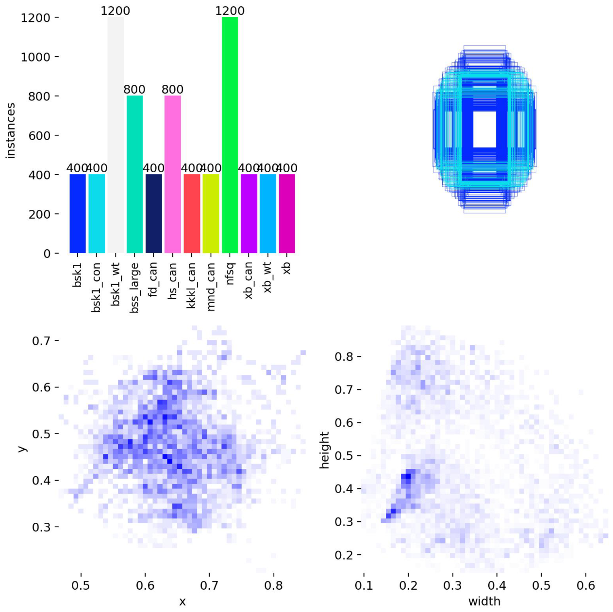
Figure 3.
Class-instance distribution and bounding-box spatial distribution of the commodity dataset. The colored bars denote class-wise instance counts, the blue rectangular outlines show normalized bounding-box coverage, and the density maps visualize box center and size distributions; darker blue indicates higher density.
Figure 3.
Class-instance distribution and bounding-box spatial distribution of the commodity dataset. The colored bars denote class-wise instance counts, the blue rectangular outlines show normalized bounding-box coverage, and the density maps visualize box center and size distributions; darker blue indicates higher density.
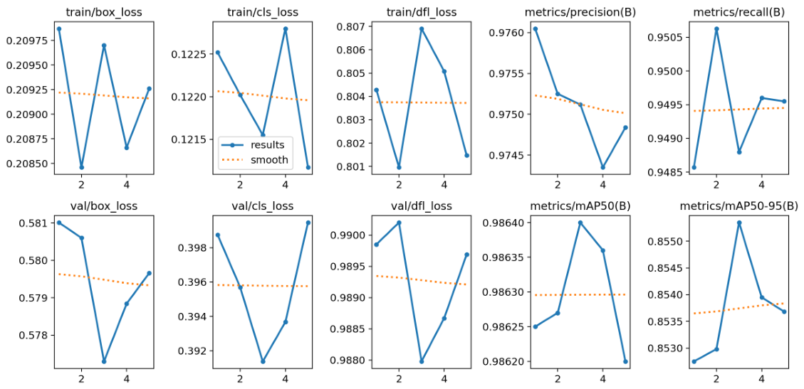
Figure 4.
Training losses and validation metrics of the final weak-class-aware fine-tuning stage. Blue solid lines are epoch-wise results, and orange dotted lines are smoothed trends; the legend does not obscure the interpretation of the metric trajectories.
Figure 4.
Training losses and validation metrics of the final weak-class-aware fine-tuning stage. Blue solid lines are epoch-wise results, and orange dotted lines are smoothed trends; the legend does not obscure the interpretation of the metric trajectories.
Figure 5.
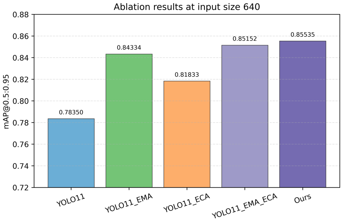
Ablation comparison of mAP50-95 for YOLO11-series models at an input size of 640.
Figure 5.
Ablation comparison of mAP50-95 for YOLO11-series models at an input size of 640.
Figure 6.
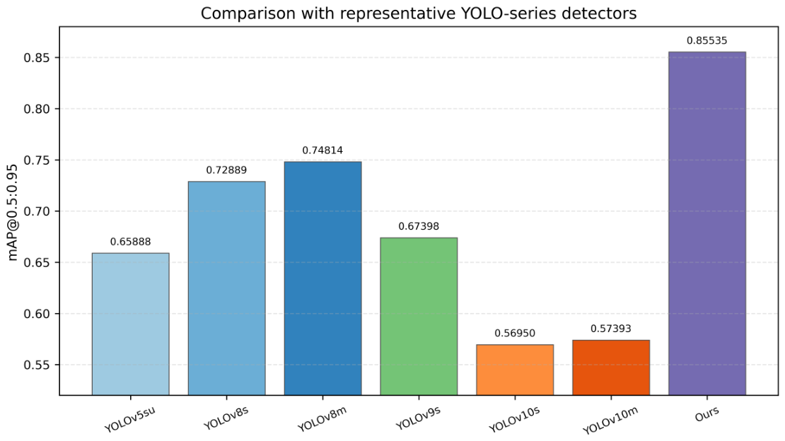
mAP50-95 comparison among representative YOLO-series detectors and the proposed method.
Figure 6.
mAP50-95 comparison among representative YOLO-series detectors and the proposed method.
Figure 7.
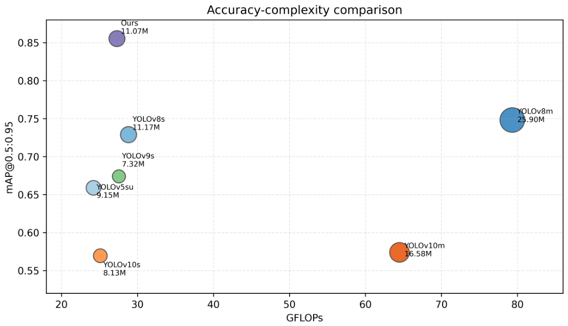
Accuracy–complexity comparison in terms of mAP50-95 and GFLOPs.
Figure 7.
Accuracy–complexity comparison in terms of mAP50-95 and GFLOPs.
Figure 8.
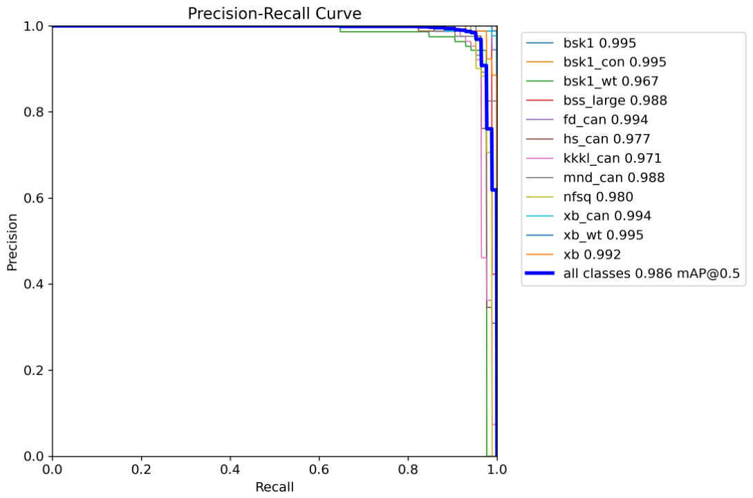
Precision–Recall curve of the final model on the validation set.
Figure 8.
Precision–Recall curve of the final model on the validation set.
Figure 9.
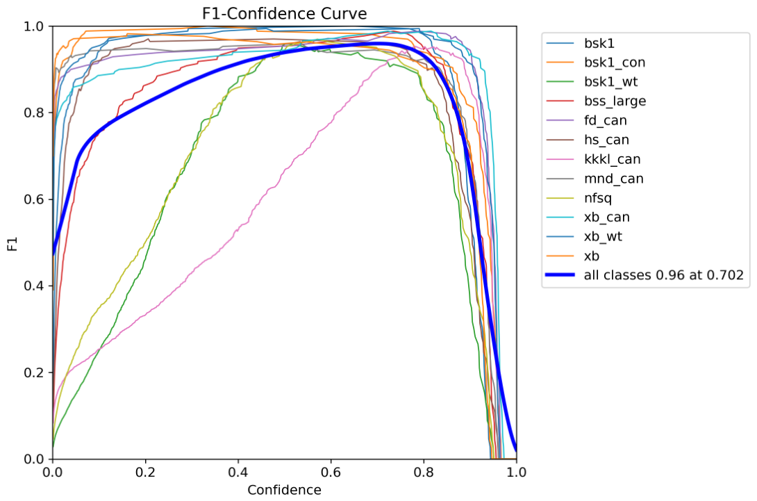
F1–Confidence curve of the final model on the validation set.
Figure 9.
F1–Confidence curve of the final model on the validation set.
Figure 10.
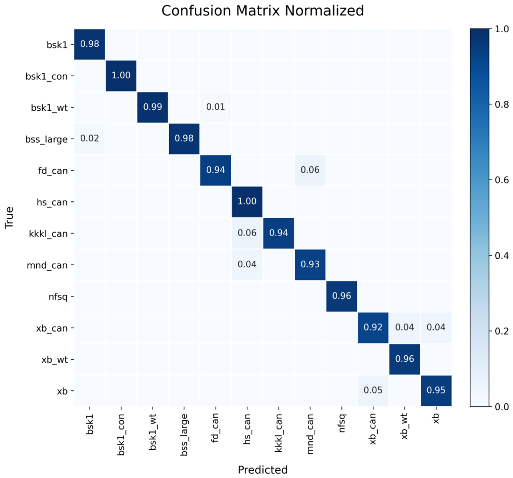
Row-normalized class-only confusion matrix of the final model. Each row is normalized to make the class-wise prediction distribution directly comparable; therefore, the displayed values remain within a valid normalized range. The background row and column are omitted for visual clarity.
Figure 10.
Row-normalized class-only confusion matrix of the final model. Each row is normalized to make the class-wise prediction distribution directly comparable; therefore, the displayed values remain within a valid normalized range. The background row and column are omitted for visual clarity.
Figure 11.
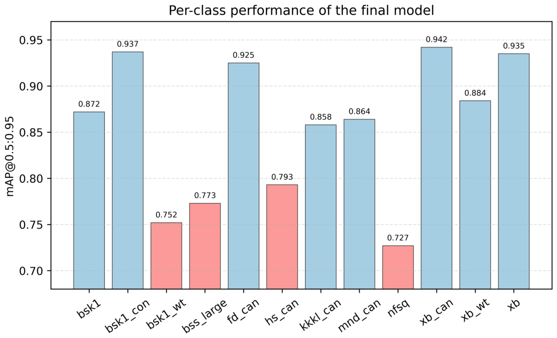
Per-class mAP50-95 of the final model on the 12 commodity categories.
Figure 11.
Per-class mAP50-95 of the final model on the 12 commodity categories.
Figure 12.
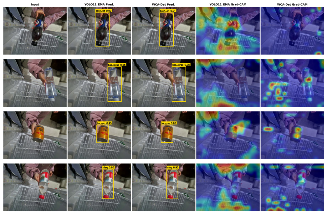
Side-by-side Grad-CAM comparison on representative weak-class samples. For each sample, the prediction and activation map of YOLO11_EMA are compared with those of WCA-Det. The comparison shows that WCA-Det generally produces more compact responses on product bodies, labels, and local package textures, while individual cases may still exhibit dispersed attention. The heat-map colors follow the standard Grad-CAM convention, where warmer colors indicate stronger activation. Dataset class identifiers such as bsk1_wt and nfsq are kept as category codes and do not affect reading.
Figure 12.
Side-by-side Grad-CAM comparison on representative weak-class samples. For each sample, the prediction and activation map of YOLO11_EMA are compared with those of WCA-Det. The comparison shows that WCA-Det generally produces more compact responses on product bodies, labels, and local package textures, while individual cases may still exhibit dispersed attention. The heat-map colors follow the standard Grad-CAM convention, where warmer colors indicate stronger activation. Dataset class identifiers such as bsk1_wt and nfsq are kept as category codes and do not affect reading.
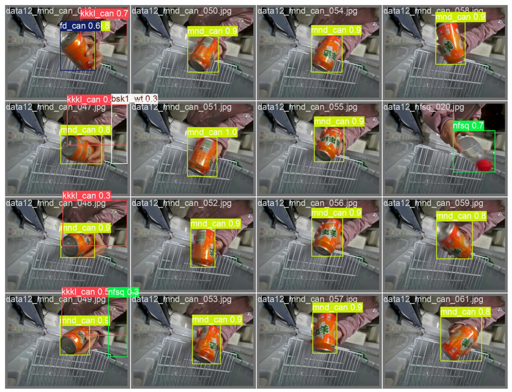
Figure 13.
Detection examples of the final model on commodity samples. The class identifiers shown in the predicted boxes are dataset category codes.
Figure 13.
Detection examples of the final model on commodity samples. The class identifiers shown in the predicted boxes are dataset category codes.
Table 1.
Structural clarification of the modified high-level attention stage.
Table 1.
Structural clarification of the modified high-level attention stage.
| Model Variant | Layer-10 Replacement | ECA Position | Counted Block/Stage | Params |
|---|
| YOLO11 | C2PSA | – | Original high-level C2PSA block at layer 10 | 1,455,616 |
| YOLO11_EMA | EMA | – | C2PSA replaced by the lightweight EMA block | 82,432 |
| YOLO11_ECA | C2PSA | Layer 22 | Original layer-22 C3k2 block plus the attached ECA kernel | 2,365,443 |
| YOLO11_EMA_ECA | EMA | After EMA | Layer-10 EMA block plus a lightweight ECA kernel | 82,435 |
Table 2.
Weak-class augmentation configuration used in the final training stage.
Table 2.
Weak-class augmentation configuration used in the final training stage.
| ID | Class | Original | Added | Multiplier | Offline Variants |
|---|
| 2 | bsk1_wt | 400 | 800 | 3× | brightness–contrast–saturation enhancement; dim sharpening with Gaussian noise |
| 3 | bss_large | 400 | 400 | 2× | brightness–contrast–saturation enhancement |
| 5 | hs_can | 400 | 400 | 2× | brightness–contrast–saturation enhancement |
| 8 | nfsq | 400 | 800 | 3× | brightness–contrast–saturation enhancement; dim sharpening with Gaussian noise |
Table 3.
Ablation results of YOLO11-series models at an input size of 640.
Table 3.
Ablation results of YOLO11-series models at an input size of 640.
| Method | Size | Params (M) | GFLOPs | P | R | mAP50 | mAP50–95 | Gain vs. EMA |
|---|
| YOLO11 | 640 | 12.44 | 27.9 | ∼0.923 | ∼0.904 | ∼0.975 | 0.78350 | −0.05984 |
| YOLO11_EMA | 640 | 11.07 | 27.3 | 0.970 | 0.951 | 0.987 | 0.84334 | – |
| YOLO11_ECA | 640 | 12.44 | 27.9 | 0.923 | 0.904 | 0.975 | 0.81833 | −0.02501 |
| YOLO11_EMA_ECA | 640 | 11.07 | 27.3 | 0.971 | 0.948 | 0.986 | 0.85152 | +0.00818 |
| Ours | 640 | 11.07 | 27.3 | 0.975 | 0.949 | 0.986 | 0.85535 | +0.01201 |
Table 4.
Seed-repeat stability of the final weak-class-aware fine-tuning stage.
Table 4.
Seed-repeat stability of the final weak-class-aware fine-tuning stage.
| Run | Best Epoch | P | R | mAP50 | mAP50–95 |
|---|
| S0 | 3 | 0.97512 | 0.94880 | 0.98640 | 0.85535 |
| S1 | 1 | 0.97512 | 0.94976 | 0.98557 | 0.85503 |
| S2 | 1 | 0.97511 | 0.94922 | 0.98661 | 0.85466 |
| Mean | – | 0.97512 | 0.94926 | 0.98619 | 0.85501 |
| Std. | – | 0.00001 | 0.00048 | 0.00055 | 0.00035 |
Table 5.
Comparison with representative YOLO-series detectors at an input size of 640.
Table 5.
Comparison with representative YOLO-series detectors at an input size of 640.
| Model | Size | Params (M) | GFLOPs | P | R | mAP50 | mAP50–95 |
|---|
| YOLOv5su | 640 | 9.15 | 24.21 | 0.651 | 0.727 | 0.753 | 0.65888 |
| YOLOv8s | 640 | 11.17 | 28.82 | 0.707 | 0.839 | 0.835 | 0.72889 |
| YOLOv8m | 640 | 25.90 | 79.32 | 0.715 | 0.801 | 0.841 | 0.74814 |
| YOLOv9s | 640 | 7.32 | 27.56 | 0.678 | 0.766 | 0.764 | 0.67398 |
| YOLOv10s | 640 | 8.13 | 25.11 | 0.587 | 0.694 | 0.689 | 0.56950 |
| YOLOv10m | 640 | 16.58 | 64.48 | 0.541 | 0.706 | 0.674 | 0.57393 |
| Ours | 640 | 11.07 | 27.30 | 0.975 | 0.949 | 0.986 | 0.85535 |
Table 6.
Cross-source overlap validation results on the independent data_6 commodity subset.
Table 6.
Cross-source overlap validation results on the independent data_6 commodity subset.
| Class | Images | Instances | P | R | mAP50 | mAP50–95 |
|---|
| all | 510 | 510 | 0.988 | 0.979 | 0.993 | 0.94156 |
| xb_can | 170 | 170 | 0.983 | 1.000 | 0.995 | 0.945 |
| xb_wt | 170 | 170 | 0.986 | 0.994 | 0.991 | 0.917 |
| xb | 170 | 170 | 0.994 | 0.942 | 0.994 | 0.963 |
Table 7.
Per-class detection results of the final model.
Table 7.
Per-class detection results of the final model.
| Class | Images | Instances | P | R | mAP50 | mAP50–95 |
|---|
| all | 1020 | 1020 | 0.975 | 0.949 | 0.986 | 0.855 |
| bsk1 | 85 | 85 | 1.000 | 0.995 | 0.995 | 0.872 |
| bsk1_con | 85 | 85 | 1.000 | 0.955 | 0.995 | 0.937 |
| bsk1_wt | 85 | 85 | 0.974 | 0.875 | 0.967 | 0.752 |
| bss_large | 85 | 85 | 0.977 | 0.988 | 0.988 | 0.773 |
| fd_can | 85 | 85 | 0.959 | 0.988 | 0.994 | 0.925 |
| hs_can | 85 | 85 | 0.988 | 0.933 | 0.977 | 0.793 |
| kkkl_can | 85 | 85 | 0.848 | 0.965 | 0.971 | 0.858 |
| mnd_can | 85 | 85 | 0.987 | 0.903 | 0.988 | 0.864 |
| nfsq | 85 | 85 | 1.000 | 0.898 | 0.980 | 0.727 |
| xb_can | 85 | 85 | 0.970 | 1.000 | 0.994 | 0.942 |
| xb_wt | 85 | 85 | 0.997 | 0.988 | 0.995 | 0.884 |
| xb | 85 | 85 | 1.000 | 0.900 | 0.992 | 0.935 |
Table 8.
Quantitative localization comparison of Grad-CAM responses on representative weak-class samples. The CAM-in-box score denotes the proportion of normalized Grad-CAM activation falling inside the ground truth product box.
Table 8.
Quantitative localization comparison of Grad-CAM responses on representative weak-class samples. The CAM-in-box score denotes the proportion of normalized Grad-CAM activation falling inside the ground truth product box.
| Class | YOLO11_EMA | WCA-Det | Gain |
|---|
| bsk1_wt | 0.229 | 0.138 | −0.092 |
| bss_large | 0.017 | 0.158 | +0.141 |
| hs_can | 0.113 | 0.176 | +0.063 |
| nfsq | 0.065 | 0.124 | +0.060 |
| Average
| 0.106 | 0.149 | +0.043 |




 ,
,