A Dynamic Displacement Measurement Method for Overhead Transmission Line Galloping Based on Deep Vision and Binocular Collaboration

Abstract

Galloping of overhead transmission lines threatens grid safety and requires non-contact measurement methods that can quantify three-dimensional (3D) motion from field video. This paper proposes a deep-vision and binocular-collaboration framework for dynamic conductor displacement measurement. The framework combines three components that are matched to the physical structure of transmission lines: adaptive image enhancement using Retinex illumination decomposition and Wiener blind deconvolution; a structure-prior dual-branch extraction module that uses an improved YOLOv11 keypoint branch for spacer-equipped sections and an improved U-Net branch with Dynamic Snake Convolution (DSC) and Strip Pooling for bare conductors; and stereo reconstruction with Kalman-filter-based temporal association for continuous trajectory estimation. Compared with the original submission, the revised manuscript further clarifies the real-video data acquisition, annotation procedure, camera synchronization, calibration workflow, training/testing independence, and runtime measurement protocol. Additional validation on a public real power-line image dataset is also reported. The proposed method achieves a Z-axis Root Mean Square Error (RMSE) of 24.5 mm for spacer sections in the controlled binocular field test, a dominant-frequency relative error below 3.5%, and 32 FPS on edge hardware when preprocessing, visual extraction, stereo projection, and temporal filtering are included. On the supplementary public power-line dataset, the segmentation branch obtains a Dice coefficient of 0.9039 and an IoU of 0.8395. These results indicate that the proposed framework reduces the depth-scale limitation of monocular vision and provides a practical quantitative tool for field galloping monitoring.

1. Introduction

Overhead transmission lines span vast geographical areas and are frequently exposed to wind, icing, low illumination, and complex backgrounds. Under winter weather, asymmetric ice accretion on conductors and ground wires, coupled with transverse wind excitation, may trigger the low-frequency and large-amplitude aeroelastic motion known as galloping [1,2]. Sustained galloping can accelerate fatigue damage of tower structures, insulator strings, and hardware fittings, and in severe cases it may contribute to conductor breakage, phase-to-phase flashover, or local tower damage [3,4]. Therefore, field monitoring systems need not only to detect whether a conductor is visible, but also to quantify its dynamic 3D displacement.

Historically, line galloping has often been monitored using contact-type mechanical or inertial sensors, such as accelerometers, strain gauges, or tilt sensors, directly mounted on conductors [5]. These sensors can provide direct local measurements, but their installation and maintenance usually require live-line work or power outages. Their energy supply and wireless transmission may also be affected by icing, weather, and electromagnetic interference in high-voltage alternating current environments [6,7].

Consequently, non-contact visual inspection technologies, particularly those empowered by Unmanned Aerial Vehicles (UAVs), have rapidly emerged as the primary means for daily smart grid maintenance. Benefiting from high mobility, safe operational distances, and global spatial observation capabilities, UAV-based vision systems have made significant breakthroughs in power line inspection [8,9]. Currently, deep learning applications in this domain have achieved remarkable success in identifying static defects, such as broken insulator sheds, missing cotter pins, and slipped Stockbridge dampers [10,11,12].

However, quantitative analysis of the dynamic galloping process remains limited compared with static defect recognition [13,14]. The transition from object recognition to trajectory measurement is difficult because bare conductors are slender, weakly textured, and often low contrast. In practical transmission corridors, camera jitter, haze, background clutter, dusk illumination, and motion blur can reduce the visibility of conductor edges, leading to feature loss, tracking drift, and trajectory fragmentation [3,8,15].

Furthermore, the vast majority of existing visual vibration measurement frameworks rely on monocular vision paradigms [5,6]. Due to the inherent lack of depth information in a single camera view, monocular systems struggle to quantify the absolute displacement of conductors in three-dimensional (3D) space. When the conductor undergoes complex spatial galloping with significant out-of-plane motion, the 2D pixel displacement cannot be accurately mapped to physical coordinates, resulting in severe scale ambiguity and unacceptable measurement errors.

The central idea of this study is that line components with different physical structures should not be forced into a single visual representation. Spacer-equipped sections provide rigid geometric anchors, whereas bare conductors require continuous pixel-level topology. At the same time, the 2D visual observations must be converted into physically meaningful 3D trajectories and temporally stabilized across video frames. Based on this idea, this paper proposes a non-contact computer vision framework for dynamic 3D galloping displacement measurement. The framework integrates existing visual modules in a task-specific way around three design principles: structure-aware feature extraction, binocular scale recovery, and temporal motion consistency. The main contributions are summarized as follows:

• Environmentally Adaptive Image Enhancement: To address optical degradation caused by field illumination variation and motion blur, an adaptive preprocessing pipeline integrating Wiener filtering blind deconvolution and Retinex illumination decomposition is introduced [16,17]. This module suppresses noise and enhances edge gradients under wind-induced blur and weak-light environments, improving the stability of subsequent feature extraction.
• Structure-Prior-Based Dual-Branch Visual Extraction: For spacer-equipped sections, a lightweight YOLOv11 keypoint branch with a Feature Pyramid Network (FPN) is designed to obtain stable geometric anchors from rigid hardware [18]. For long bare conductors, a topology-aware U-Net branch integrating Dynamic Snake Convolution (DSC) and Strip Pooling is used to segment slender curved structures at pixel level [19,20,21]. The novelty lies in matching the visual representation to the physical component: sparse keypoints for rigid spacers and continuous masks/skeletons for flexible conductors.
• 3D Spatiotemporal Reconstruction for Field Video: By coupling binocular stereo projection with cross-frame tracking based on optical flow and Kalman filtering [22,23], the system reconstructs continuous 3D conductor trajectories from video. This reduces the scale ambiguity of monocular vision and mitigates short-term trajectory fragmentation. Dynamic parameters, including 3D amplitude, dominant frequency, and spatial waveform inclination, can then be extracted [24,25] for galloping assessment.

2. Related Work

In the field of non-contact visual monitoring of transmission corridors, the core difficulties lie in the high-precision extraction of slender targets against complex backgrounds and the continuous quantification of high-frequency dynamic parameters. Existing research can be divided into three stages based on technical evolution.

2.1. Traditional Visual Feature Extraction Algorithms and Their Limitations

Early visual recognition of transmission lines primarily relied on underlying image processing technologies and hand-crafted feature operators. References [8,26] utilized Canny edge detection, Hough transform, and their improved algorithms to extract the linear or curved contours of conductors. The core mechanism of these methods relies on mapping image space edge pixels into a parameter space and accumulating local maximum votes to extract straight lines. For instance, Chen et al. [15] proposed an improved Cluster Radon Transform (CRT) to extract power lines from high-resolution remote sensing imagery. This method effectively avoids false alarms compared to conventional Radon transforms by grouping line segments, but it still relies heavily on prior linear assumptions. Reference [27] combined mathematical morphology with the region-growing method to achieve static sag measurement of conductors from specific perspectives.

However, the review in reference [1] clearly indicated that traditional feature operators highly depend on the prior contrast of images and predefined threshold settings. As typical low-contrast, textureless targets, the gradient features of overhead conductors are extremely fragile. In field conditions involving strong light reflection, smog, or low illumination, the signal-to-noise ratio drops drastically. The weak gradient features of the conductors are easily submerged by complex background clutter such as vegetation, ground buildings, or road markings, causing traditional edge detectors to yield severely fragmented contour maps.

Additionally, early vision-based Structural Health Monitoring (SHM) primarily adopted localized pattern matching and corner detection techniques to track the dynamic responses of large civil infrastructures [6,28]. While these methods achieved high sub-pixel tracking accuracy under stable laboratory lighting, they proved excessively brittle when deployed in transmission corridors. The feature points on conductors constantly experience non-rigid shape variations and severe illumination fluctuations, causing conventional tracking templates to drift or lose targets entirely.

Furthermore, in the domain of structural displacement measurement, traditional methods heavily relied on two-dimensional Digital Image Correlation (DIC) [29]. DIC tracks physical displacement by calculating the cross-correlation coefficient of image subsets before and after deformation. While DIC offers sub-pixel accuracy, it strictly requires distinct surface speckle patterns or artificial targets to perform block-matching. Since bare overhead conductors inherently lack surface textures and present uniform specular reflections under sunlight, the correlation calculation often falls into local optima. Considering that installing artificial markers on high-voltage lines is highly impractical and dangerous, DIC and other template-matching methods exhibit poor generalization and robustness, ultimately failing to meet the all-weather, marker-free engineering monitoring requirements of field transmission lines.

2.2. Application and Bottlenecks of Deep Learning in Transmission Inspection

The introduction of Convolutional Neural Networks (CNNs) has revolutionized the intellectualization of grid inspection by shifting from hand-crafted geometric features to data-driven semantic representations. Two-stage detection networks, represented by Faster R-CNN [30], introduced Region Proposal Networks (RPNs) to automatically generate candidate boxes, achieving high-precision localization. References [10,11] verified its robustness in recognizing rigid defects such as insulator breakage and Stockbridge damper slippage against complex backgrounds. However, two-stage networks are computationally expensive and struggle with real-time video stream processing.

To meet the real-time inference requirements of UAV-borne equipment with strictly limited computing power, single-stage lightweight detectors, represented by YOLO [31] and SSD, were widely adopted. By framing object detection as a single end-to-end regression problem, references [9,12] significantly improved the computational efficiency of hardware recognition. While these standard detection networks excel at category identification, they are mostly based on the Bounding Box Regression mechanism [32]. This paradigm presents inherent geometric defects when processing bare conductors with extreme aspect ratios. Rectangular bounding boxes inherently force the network to enclose the slender target, meaning that over 90% of the pixels inside the bounding box are background noise. This severe class imbalance inside the box leads to poor convergence of Intersection over Union (IoU) losses and fails to provide pixel-level topological structures.

To achieve finer extraction, instance segmentation models like Mask R-CNN [33] were developed to provide pixel-level masks alongside bounding boxes via the RoIAlign operation. However, their heavy multi-branch architectures further exacerbate the computational burden. More recently, the introduction of Vision Transformers has disrupted the object detection landscape. Models such as DETR (Detection Transformer) [34] eliminate the need for hand-crafted components like non-maximum suppression by framing detection as a direct set prediction problem. Although Transformer-based architectures have achieved state-of-the-art accuracy in complex scene understanding, their self-attention mechanisms introduce quadratic computational complexity with respect to the input spatial resolution. This massive computational overhead makes high-frame-rate tracking on airborne edge devices nearly impossible.

Furthermore, for tracking rigid structures like spacers in vibrating environments, dense pixel masks are often redundant. Instead, keypoint-based localization offers a more sparse yet geometrically stable representation [35]. Achieving high-precision keypoint regression under multi-scale variations remains a challenge, motivating the integration of specialized feature pyramids (FPNs) in our proposed lightweight YOLOv11 branch to decouple rigid component tracking from flexible conductor extraction while maintaining strict real-time efficiency.

2.3. Slender Target Segmentation and 3D Dynamic Tracking

To address the pixel-level localization bottleneck of flexible conductors, Fully Convolutional Networks (FCNs) [36] and semantic segmentation architectures have been introduced. Classic encoder–decoder networks, such as U-Net [19] and SegNet [37], utilize successive downsampling layers to capture rich global context and upsampling layers with skip connections to recover spatial resolution.

To address objects with diverse scales and extreme aspect ratios, advanced multi-scale feature aggregation architectures, such as Panoptic Feature Pyramid Networks (Panoptic FPN) [38], have been developed. While these architectures successfully unify instance and semantic segmentation by merging dense bottom-up features with semantic top-down pathways, they still fundamentally rely on regular grid convolutions. When applied to extremely slender power lines, these square receptive fields inadvertently incorporate excessive background features from adjacent regions. When the conductor undergoes non-linear bending due to wind-induced galloping, this structural mismatch leads to severe false positives or trajectory disconnections at conductor overlaps. To elegantly address this, references [20,21] proposed enhancing the network’s local geometric perception for slender, curved targets through Strip Pooling and Dynamic Snake Convolution (DSC). These operators dynamically adapt their receptive fields to strictly align with the tubular structures, effectively filtering out off-axis background interference.

Despite advancements in 2D target extraction, dynamic displacement measurement still faces significant physical hurdles. Vision-based Structural Health Monitoring (SHM) has made great progress [14,39], leveraging deep neural networks for multi-scale structural inspection [40]. Yet, most visual vibration measurement technologies are confined to monocular 2D planar estimation. Reference [3] utilized the optical flow method for sub-pixel modal vibration measurement. However, monocular methods suffer from severe scale ambiguity due to the inherent loss of depth information, especially when conductors exhibit large out-of-plane galloping motions where the absolute distance between the camera and the target changes constantly [6].

Binocular stereo vision reduces this scale ambiguity by recovering absolute spatial depth through epipolar geometry constraints. Recent geometric-vision studies on multi-camera and generalized-camera relative pose estimation have further improved the mathematical basis of calibrated multi-camera measurement. For example, affine-correspondence-based methods and six-point solvers reduce the required correspondence set and improve pose-estimation efficiency in multi-camera systems [41,42,43]. These studies are highly relevant to visual displacement measurement because accurate camera pose and correspondence estimation are prerequisites for reliable 3D reconstruction. The focus of this paper is different: instead of proposing a new minimal relative-pose solver, we use a calibrated binocular rig and task-specific conductor features to recover dynamic line trajectories in field video.

Nevertheless, standard stereo matching algorithms [44,45] typically rely on local patch-based cost aggregation (e.g., Sum of Absolute Differences or Normalized Cross-Correlation). When attempting to match weakly textured bare conductors against complex, low-contrast sky backgrounds, the cost volume often becomes flat. This leads to disparity discontinuities or “depth holes.” Moreover, airborne jitter and brief target occlusion under complex meteorology cause tracking losses. Therefore, bridging the disparity discontinuities of textureless conductors and maintaining the spatiotemporal consistency of dynamic tracking through cross-frame state estimation (e.g., Kalman filtering [22]) remains the task-specific technical gap that this paper aims to address.

3. Method

This paper proposes a non-contact visual galloping displacement measurement framework. The framework is cooperatively composed of three core modules: complex environment adaptive image enhancement, structure-prior-based dual-branch target extraction networks, and binocular-disparity-based spatiotemporally consistent trajectory reconstruction.

3.1. Adaptive Image Enhancement Under Complex Illumination and Meteorological Conditions

Due to the uncontrollability of field monitoring scenarios, acquired images are often accompanied by low-illumination noise and severe motion blur. To ensure the accuracy of subsequent feature extraction algorithms, the system first executes an adaptive preprocessing pipeline at the data input end.

Low-Illumination Compensation and Denoising: For nighttime and weak-light environments, the system adopts an illumination decomposition algorithm based on Retinex theory [16] to separate the reflection and illumination components of the image. This is combined with Contrast-Limited Adaptive Histogram Equalization (CLAHE) [46] to enhance local texture details. To address Poisson noise caused by high-gain exposure, Non-Local Means (NLM) filtering [47] is introduced to maximize the retention of the extremely thin edge gradients of conductors while smoothing background noise. Unlike traditional local filters that blur structural boundaries, NLM computes the filtered pixel value as a weighted average of all pixels in the image, where the weights are determined by the similarity of their surrounding geometric neighborhoods, effectively preserving the topological integrity of the wire edges.

Motion Blur Restoration: In scenarios involving high-frequency UAV camera jitter caused by strong winds or severe conductor galloping, target edges suffer from severe point spread degradation. This paper employs Wiener filtering combined with the Blind Deconvolution algorithm [17] to inversely solve motion-blurred images by iteratively estimating the unknown Point Spread Function (PSF), effectively restoring high-frequency edge features. Through an iterative maximum likelihood estimation, the algorithm refines the PSF estimate alongside the latent image until convergence is achieved.

For low-illumination compensation, the Retinex theory assumes that an image $I(x,y)$ can be modeled as the product of the illumination component $L(x,y)$ and the reflection component $R(x,y)$:

$$I(x,y)=L(x,y)·R(x,y)$$

By transforming this into the logarithmic domain, the reflection component, which represents the intrinsic properties of the conductors, can be isolated:

$$\log R(x,y)=\log I(x,y)-\log \left(F\right(x,y)\ast I(x,y\left)\right)$$

where $F(x,y)$ is a Gaussian surround function utilized to estimate the illumination distribution.

For motion blur restoration, the degradation process of the image caused by high-frequency jitter can be modeled as:

$$g(x,y)=f(x,y)\ast h(x,y)+n(x,y)$$

where $g(x,y)$ is the blurred image, $f(x,y)$ is the latent clear image, $h(x,y)$ represents the unknown Point Spread Function (PSF), and $n(x,y)$ is additive noise. A Wiener filter is applied in the frequency domain to perform the inverse solution:

$$\widehat{F}(u,v)=\left[{\displaystyle \frac{H^{\ast }(u,v)}{{\left|H(u,v)\right|}^2+K}}\right]G(u,v)$$

where $\widehat{F}(u,v)$, $G(u,v)$, and $H(u,v)$ are the Fourier transforms of $\widehat{f}$, g, and h, respectively. $H^{\ast }$ is the complex conjugate of H, and K is a constant related to the signal-to-noise ratio.

3.2. Structure-Prior-Based Dual-Branch Slender Target Extraction Network

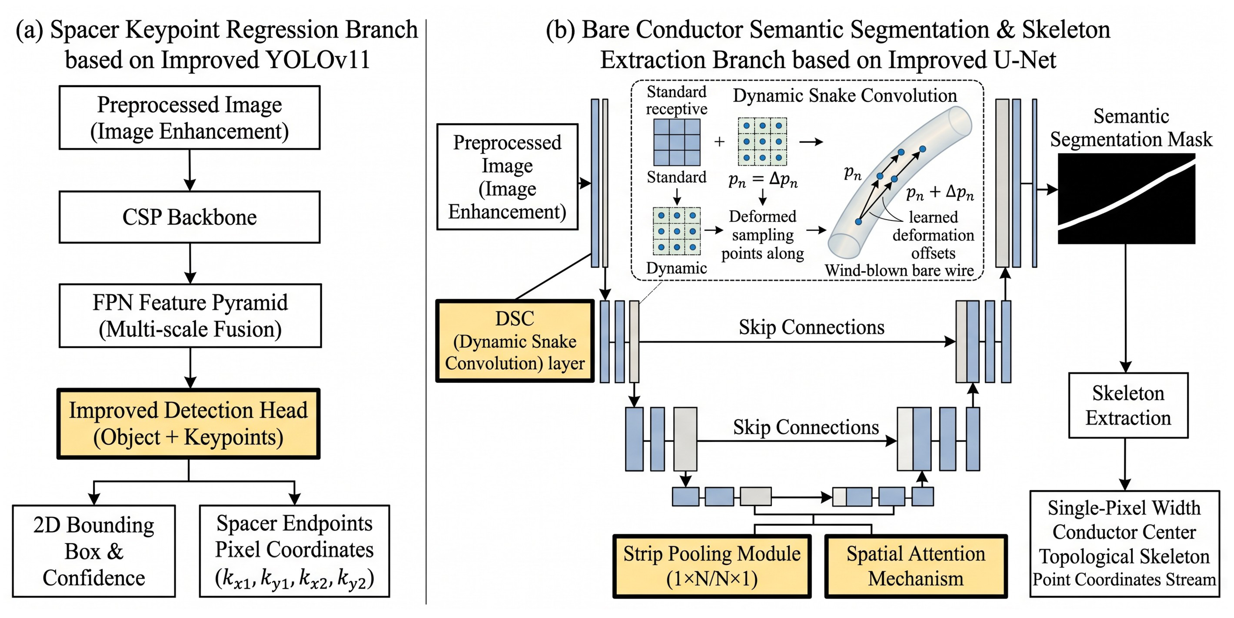
Transmission lines present two distinctly different physical morphologies: “with hardware (spacers)” and “without hardware (bare conductors).” A single detection network cannot accommodate both local keypoint localization and global pixel segmentation simultaneously. Therefore, a dual-branch visual detection strategy is designed for different line topologies, as illustrated in Figure 1.

3.2.1. Lightweight Keypoint Detection for Spacers

For sections installed with spacers, the geometric morphology of the spacers provides a high-contrast rigid observation baseline for conductor tracking. Based on the YOLO architecture, this paper integrates a Feature Pyramid Network (FPN) [18] to enhance the cross-layer fusion of multi-scale features. As depicted in Figure 1a, the detection pipeline leverages a Cross Stage Partial (CSP) backbone for efficient feature extraction. To handle the significant scale variations in spacers caused by dynamically changing UAV flight distances, the FPN aggregates semantic information from deep layers with high-resolution spatial details from shallow layers.

The detection head is specifically modified to not only regress the 2D bounding boxes $(x,y,w,h)$ of targets and confidence scores, but also to output the precise pixel coordinates of the upper and lower endpoints $(k_{x1},k_{y1},k_{x2},k_{y2})$ of the spacers. To optimize the keypoint regression, a composite loss function is employed, combining bounding box regression loss with a normalized keypoint distance loss. This ensures that the gradient descent process prioritizes the alignment of the spacer’s structural joints over merely minimizing the bounding box scale error. These predicted keypoints serve as highly stable geometric anchors for subsequent spatial posture calculation, overcoming the inherent instability of traditional bounding box centers during hardware vibration. Through channel pruning and weight quantization, the model reduces computational redundancy and meets real-time inference requirements on airborne edge computing nodes.

3.2.2. Topology-Aware Semantic Segmentation for Bare Conductors

For extremely slender, low-contrast bare conductors without spacers, the traditional bounding box detection paradigm easily introduces background interference, since the target occupies only a fraction of the box area. This paper adopts an improved U-Net segmentation model [19], as detailed in Figure 1b. The network follows an encoder–decoder paradigm with skip connections to preserve fine-grained spatial features. Crucially, introducing DSC [21] in its encoder stage allows it to adaptively match the nonlinear curved morphology of conductors affected by wind deflection by learning deformation offsets.

In standard 2D convolution, the output feature map Y at location $p_0$ is computed by sampling the input feature map X over a regular grid $\mathcal{R}$ with weights w:

$$Y\left(p_0\right)=\sum _{p_n\in \mathcal{R}}w\left(p_n\right)·X(p_0+p_n)$$

However, bare conductors constantly undergo nonlinear bending due to wind deflection, making regular rigid grids ineffective. The Dynamic Snake Convolution (DSC) introduces learned 2D offsets $\Delta p_n$ to the regular grid, enabling the receptive field to dynamically align with the tubular topological structure of the conductor:

$$Y\left(p_0\right)=\sum _{p_n\in \mathcal{R}}w\left(p_n\right)·X(p_0+p_n+\Delta p_n)$$

where the offset $\Delta p_n$ is generated by an additional convolutional layer applied over the same input feature maps. This mechanism allows the network to adaptively focus on the continuous slender features while suppressing surrounding background noise.

Concurrently, combined with a Strip Pooling module [20] and a spatial attention mechanism, it captures the long-distance contextual dependencies of slender targets. Unlike traditional spatial pooling with square windows, Strip Pooling utilizes long, narrow pooling kernels (e.g., $1\times N$ and $N\times 1$). Mathematically, given a 2D tensor $X\in {\mathbb{R}}^{H\times W\times C}$, the horizontal strip pooling computes the mean value of a row, yielding a 1D vector $y^h\in {\mathbb{R}}^{H\times 1\times C}$, while vertical strip pooling yields $y^v\in {\mathbb{R}}^{1\times W\times C}$. These orthogonal features are expanded and fused to form a global receptive field that is highly sensitive to the continuous topological layout of the power lines without absorbing unnecessary background clutter. The combined architecture ultimately outputs a highly continuous mask, which is processed via morphological thinning to yield a single-pixel-width conductor center topological skeleton.

3.3. Spatial Trajectory Reconstruction and Dynamic Parameter Temporal Quantification

After obtaining stable 2D pixel coordinates or skeleton lines, the system achieves 2D-to-3D dynamic displacement quantification through stereo matching and temporal state estimation algorithms.

3.3.1. Stereo Matching and 3D Spatial Projection

The system calculates sub-pixel dense disparity maps for binocular views via Semi-Global Block Matching (SGBM) [23] or stereo matching networks (e.g., PSMNet) [24]. To suppress disparity discontinuities commonly found in textureless conductor surfaces, the SGBM algorithm optimizes a global energy function $E\left(D\right)$ across the disparity map D:

$$E\left(D\right)=\sum _p\left(C(p,D_p)+\sum _{q\in N_p}{P}_{1}I\left(\right|D_p-D_q| =1)+\sum _{q\in N_p}{P}_{2}I\left(\right|D_p-D_q| >1)\right)$$

where $C(p,D_p)$ is the initial matching cost at pixel p for disparity $D_p$, $N_p$ is the neighborhood of p, and $P_1,P_2$ are empirically set penalty parameters for small and large disparity gradients, respectively, ensuring surface smoothness for the extracted targets.

Based on the binocular pinhole camera model and epipolar geometry principles, the absolute spatial depth $Z_c$ of a target point in the camera coordinate system can be calculated by:

$$Z_c={\displaystyle \frac{f·b}{d}}$$

where f is the effective focal length of the camera, b is the baseline length of the binocular camera, and $d=u_{left}-u_{right}$ is the corresponding horizontal disparity value between the left and right views.

Once the depth $Z_c$ is obtained, the 2D pixel coordinates $(u,v)$ are back-projected into 3D coordinates $(X_c,Y_c,Z_c)$ within the local camera coordinate system using the camera intrinsic parameters:

$$X_c={\displaystyle \frac{(u-c_x)·Z_c}{f_x}},Y_c={\displaystyle \frac{(v-c_y)·Z_c}{f_y}}$$

where $(c_x,c_y)$ is the principal point of the image, and $f_x,f_y$ are the focal lengths along the pixel axes.

It should be noted that the source of the 2D coordinate $(u,v)$ depends on the active detection branch: for the spacer section, $(u,v)$ represents the geometric center of the keypoints detected by YOLOv11, and for the bare conductor section, $(u,v)$ represents the extracted skeleton points from the improved U-Net. This unified projection mechanism ensures that both rigid and flexible components can be reconstructed in the same 3D spatial framework.

Finally, the local coordinates are unified into the global geographic coordinate system $(X_w,Y_w,Z_w)$ via homogeneous coordinate transformation combined with airborne pose information (RTK/IMU):

$$\left[\begin{array}{c}{X}_w\\ Y_w\\ Z_w\\ 1\end{array}\right]={\mathbf{T}}_{IMU}^{World}\left[\begin{array}{cc}\mathbf{R}& \mathbf{t}\\ \mathbf{0}& 1\end{array}\right]\left[\begin{array}{c}{X}_c\\ Y_c\\ Z_c\\ 1\end{array}\right]$$

where $\mathbf{R}$ and $\mathbf{t}$ denote the rotation matrix and translation vector respectively.

3.3.2. Calibration, Synchronization, and Ground-Truth Alignment

To make the stereo measurement process reproducible, the binocular system is calibrated before field acquisition using a planar checkerboard target observed at multiple distances and orientations. The intrinsic parameters of the left and right cameras, distortion coefficients, stereo rotation, and stereo translation are estimated jointly, and the calibration is accepted only when the mean reprojection error is below one pixel. The rectified left–right image pairs are then used for the disparity calculation described above. In the field videos used in this study, the camera platform was kept stationary or in a hovering fixed-point state during each measurement sequence, so the observed image motion is dominated by conductor motion rather than intentional camera translation. Residual camera vibration is handled by feature-based background stabilization before conductor tracking.

The left and right image streams are hardware-triggered by the same acquisition controller when available; otherwise, frame timestamps are aligned before processing and frame pairs with excessive timestamp deviation are discarded. The dynamic displacement ground truth for the controlled field test is obtained by combining a Leica Nova TS60 total station and an RTK module. The total station records the 3D coordinates of selected conductor or spacer characteristic points, and the RTK/IMU records the camera pose used to transform local camera coordinates into the global coordinate system. The visual coordinate system and the survey coordinate system are aligned using common reference points on the tower or conductor fittings. Measurement uncertainty is mainly introduced by stereo calibration residuals, timestamp alignment error, manual/automatic reference-point localization, and total-station observation error; therefore, the reported ranging results are interpreted as field-test accuracy under the stated acquisition conditions rather than a universal accuracy guarantee for all corridor distances and weather conditions.

3.3.3. Cross-Frame Trajectory Association and Galloping Parameter Extraction

To address the problem of temporal fragmentation caused by large-scale conductor flipping or brief occlusions, this paper combines the optical flow method [3] and the Kalman Filter [22] for motion state prediction and data association. The state vector is defined as ${\mathbf{x}}_k={[X,Y,Z,\dot{X},\dot{Y},\dot{Z}]}^T$, which represents the 3D position and velocity of the conductor.

Specifically, for a constant velocity kinematic model with time step $\Delta t$, the state transition matrix $\mathbf{A}$ and observation matrix $\mathbf{H}$ are defined as:

$$\mathbf{A}=\left[\begin{array}{cc}{\mathbf{I}}_{3\times 3}& \Delta t{\mathbf{I}}_{3\times 3}\\ {\mathbf{0}}_{3\times 3}& {\mathbf{I}}_{3\times 3}\end{array}\right],\mathbf{H}=\left[\begin{array}{cc}{\mathbf{I}}_{3\times 3}& {\mathbf{0}}_{3\times 3}\end{array}\right]$$

The state transition and observation models are formulated as:

$${\mathbf{x}}_{k|k-1}=\mathbf{A}{\mathbf{x}}_{k-1|k-1}+{\mathbf{w}}_k$$

$${\mathbf{z}}_k=\mathbf{H}{\mathbf{x}}_{k|k-1}+{\mathbf{v}}_k$$

where ${\mathbf{z}}_k$ represents the 3D coordinates obtained from the binocular matching at frame k. ${\mathbf{w}}_k$ and ${\mathbf{v}}_k$ denote the process and measurement noise covariance matrices, respectively.

The optimal state estimate is iteratively updated using the Kalman gain ${\mathbf{K}}_k$:

$${\mathbf{x}}_{k|k}={\mathbf{x}}_{k|k-1}+{\mathbf{K}}_k({\mathbf{z}}_k-\mathbf{H}{\mathbf{x}}_{k|k-1})$$

This mechanism ensures the spatiotemporal continuity of the 3D trajectory. After obtaining the continuous trajectory, a Savitzky–Golay smoothing filter [25] is first applied to suppress high-frequency observation noise. Subsequently, the vertical and horizontal galloping amplitudes are calculated from the range of the 3D coordinate sequence. The Fast Fourier Transform (FFT) is then utilized to convert the time-domain displacement signal into the frequency domain to extract the dominant galloping frequency. Finally, the waveform inclination angle of the galloping trajectory is analyzed through spatial ellipse fitting, outputting the complete set of galloping feature parameters.

4. Experiments

To verify the proposed visual measurement framework, systematic quantitative and qualitative experiments were conducted on self-built field/simulation videos and on an additional public real power-line image dataset. To align with the dual-branch architecture proposed in Section 3, the evaluations are categorized into two typical scenarios: sections with hardware (spacers) and sections without hardware (bare conductors).

4.1. Experimental Environment and Dataset Construction

The offline training and testing environment for the algorithm was configured as follows: Intel(R) Xeon(R) Platinum 8360Y CPU operating at 2.40 GHz, NVIDIA RTX 4090 (24 GB VRAM) GPU, and PyTorch 1.13.1+cu117 deep learning framework. To verify airborne real-time performance, edge-end inference testing was conducted on an NVIDIA Jetson AGX Xavier.

To ensure the reproducibility of the visual networks, the training hyper-parameters were set as follows: the AdamW optimizer was adopted with an initial learning rate of $1\times {10}^{-4}$ and a weight decay of $1\times {10}^{-4}$. A cosine annealing learning rate scheduler was applied. The batch size was set to 16, and the models were trained for 150 epochs until the validation loss no longer decreased. For all comparative models, the same preprocessing pipeline, image resolution, dataset split, optimizer settings, and Jetson AGX Xavier deployment environment were used unless otherwise stated. The main experiments were repeated three times with different random seeds, and the tables report the mean values.

Due to the sudden and unrepeatable nature of transmission line galloping, real galloping data is scarce. This paper constructed a mixed dataset containing a total of 15,000 extracted image frames, which were strictly divided into training (70%, 10,500 frames), validation (20%, 3000 frames), and testing (10%, 1500 frames) sets. To avoid scene leakage, frames from the same continuous video segment were assigned to only one subset. The test subset contains video segments that are independent of the training and validation scenes. The data sources include:

• Digital Twin Simulation Set: A 3D scene of a transmission corridor was constructed using a physical simulation engine to simulate conductor motion under different wind speeds. Video sequences containing known camera intrinsics, extrinsics, and absolute 3D target coordinates were synthesized, generating 120 video segments. These simulated data were mainly used for pretraining, ablation, and controlled error analysis, not as the only evidence for field performance.
• Field Measurement Set: Real test data were acquired from field videos of conductor motion. During each sequence, the camera was kept fixed or in a hovering fixed-point state, so the data record conductor motion while reducing intentional camera translation. The videos include spacer-equipped conductors and bare conductor sections under clear daytime, weak-light, and wind-blur conditions. The images used in the manuscript are not isolated photographs; they are screenshots from the running measurement system when processing field video streams. To obtain physical ground truth in the controlled field tests, a Leica Nova TS60 high-precision total station combined with an RTK module was deployed on the ground to record 3D coordinates of selected characteristic points. The visual measurements and survey measurements were synchronized by acquisition timestamps and aligned through common reference points.
• Public Real Power-Line Dataset: To further evaluate generalization on real non-synthetic images, the bare-conductor segmentation branch was additionally tested on a public powerline dataset Computer Vision Dataset. This dataset is independent of the training videos used in the main experiments. Since the public dataset provides 2D line annotations but not binocular depth ground truth, it is used only to assess segmentation generalization, not 3D ranging accuracy.

To improve traceability of the real-data evaluation,

Table 1. Traceability of the Controlled Field-Test Data and Stereo Evaluation.

Item	Status in This Study
Data type for final evaluation	Real field videos of conductor motion; synthetic videos were used for pretraining, ablation, and controlled error analysis.
Camera state during each sequence	Fixed or hovering fixed-point acquisition; residual platform vibration was compensated by background stabilization.
Training/testing independence	Continuous video segments were assigned to only one subset to reduce scene leakage.
Ground-truth source	Leica Nova TS60 total-station measurements combined with RTK/IMU pose information and common reference-point alignment.
Stereo calibration record	Checkerboard calibration with intrinsic/extrinsic estimation, stereo rectification, and mean reprojection error below one pixel.
Runtime protocol	The reported 32 FPS includes preprocessing, visual extraction, stereo projection, Kalman filtering, and dynamic-parameter calculation on Jetson AGX Xavier.
Public real-data validation	Independent public power-line images were used for 2D segmentation validation only because synchronized binocular depth ground truth is unavailable.
Unrecorded hardware metadata	Exact field of view, pixel angular spacing, full target-depth distribution, and conductor pixel-width distribution were not fully retained in the available field log.

summarizes the acquisition and validation information available for the controlled field videos. Parameters not preserved in the original field log are explicitly marked rather than inferred retrospectively.

For the manual annotation of field videos, conductor masks were labeled at pixel level and spacer endpoints were labeled as keypoints. Ambiguous frames with heavy occlusion, severe defocus, or impossible conductor-boundary judgment were reviewed twice before inclusion. The final masks were checked by overlay inspection, and a subset was re-labeled to verify annotation consistency.

4.2. Evaluation Metrics

This paper evaluates the system performance from two dimensions: visual target extraction and physical displacement measurement.

• Visual Extraction Metrics: To evaluate the slender target segmentation performance of bare conductors, the mean Intersection over Union (mIoU) and Pixel Accuracy (PA) are adopted. Assuming there are $N+1$ classes (including the background), mIoU is defined as:

  $$\mathrm{mIoU}={\displaystyle \frac{1}{N+1}}{\displaystyle \sum _{i=0}^N}{\displaystyle \frac{T{P}_i}{T{P}_i+F{P}_i+F{N}_i}}$$

  where $T{P}_i$, $F{P}_i$, and $F{N}_i$ denote the number of true positive, false positive, and false negative pixels for class i, respectively. For spacer keypoint detection, the mean Average Precision at IoU thresholds of 0.5 (mAP@0.5) and the more stringent 0.5 to 0.95 (mAP@0.5:0.95) are utilized as primary metrics. To comprehensively assess hardware deployment feasibility, computational complexity (GFLOPs) and VRAM usage (MB) are also reported.
• Dynamic Measurement Metrics: To quantify the absolute ranging accuracy of the reconstructed 3D trajectories against the Ground Truth, the Root Mean Square Error (RMSE) and Mean Absolute Error (MAE) are employed:

  $$\mathrm{RMSE}=\sqrt{{\displaystyle \frac{1}{M}}\sum _{t=1}^M{(D_t-{\widehat{D}}_t)}^2}$$

  $$\mathrm{MAE}={\displaystyle \frac{1}{M}}{\displaystyle \sum _{t=1}^M}|D_t-{\widehat{D}}_t|$$

  where M is the total number of sampled frames, $D_t$ is the ground truth displacement at frame t, and ${\widehat{D}}_t$ is the system’s measured displacement. Furthermore, the Relative Error (RE) is used to evaluate the calculation accuracy of the dominant galloping frequency:

  $$\mathrm{RE}={\displaystyle \frac{|f_m-f_t|}{f_t}}\times 100\%$$

  where $f_m$ is the measured frequency derived from the FFT, and $f_t$ is the theoretical true frequency.

4.3. Performance Evaluation of Visual Detection and Segmentation Algorithms

To verify the effectiveness of the proposed dual-branch network and environmental preprocessing modules, systematic ablation experiments and comparative analyses with mainstream algorithms were conducted.

4.3.1. Ablation Validation of Complex Environment Adaptive Preprocessing

To verify the effectiveness of the environmental preprocessing pipeline proposed in Section 3.1, ablation experiments were constructed as shown in

Table 2. Ablation Experiments of Image Preprocessing Algorithms. ✓ indicates that the corresponding module is used, and ✕ indicates that it is not used.

Retinex	Wiener	Spacer	Spacer	Conductor	Inference
Comp.	Deconv.	mAP@0.5 (%)	mAP@0.5:0.95 (%)	mIoU (%)	FPS
✕	✕	68.5	45.2	65.2	42
✓	✕	76.8	52.1	74.1	38
✕	✓	74.2	55.4	72.5	35
✓	✓	80.9	61.3	80.4	32

.

As shown in Table 2, in the Baseline without any preprocessing, the model’s metrics performed poorly, limited by extremely low contrast and edge point spread degradation. The strict mAP@0.5:0.95 was only 45.2%, indicating unstable keypoint localization. When the complete adaptive preprocessing pipeline was introduced, the mAP@0.5 and mIoU increased substantially by 12.4% and 15.2%, respectively. Although the preprocessing steps sacrificed approximately 10 FPS, the overall frame rate of 32 FPS still meets airborne real-time requirements.

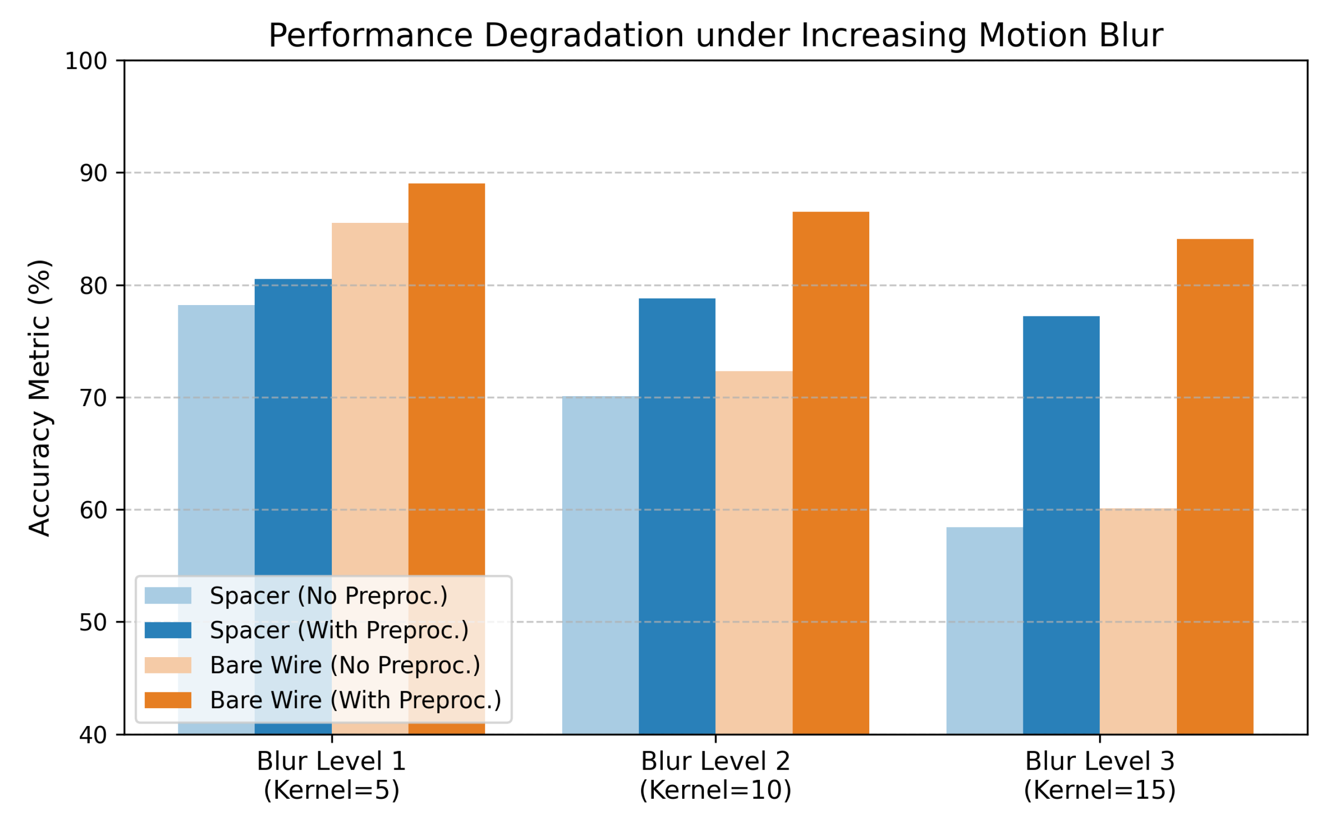
Figure 2 further illustrates the performance degradation of the dual-branch models under increasing motion blur, with and without the adaptive preprocessing pipeline.

4.3.2. Ablation Experiments of Spacer Keypoint Detection Network (YOLO Branch)

To validate the structural improvements in the YOLOv11-based spacer detection branch, an ablation study was conducted (

Table 3. Ablation Experiments of YOLOv11 Improvements for Spacer Anchoring. Bold values indicate the best performance in each metric.

Model Configuration	mAP@0.5 (%)	mAP@0.5:0.95 (%)	GFLOPs	VRAM (MB)
Baseline (Standard YOLOv11)	75.1	48.3	10.2	650
+ FPN (Feature Pyramid)	78.4	55.6	11.5	780
+ FPN + Keypoint Head (Ours)	80.9	61.3	12.4	815

). The baseline was the standard YOLOv11 model.

The introduction of FPN significantly enhanced multi-scale perception during drone approaching maneuvers. Most importantly, replacing the standard bounding box head with the customized keypoint regression head sharply increased the strict mAP@0.5:0.95 from 55.6% to 61.3%, proving its superiority in maintaining stable anchor points during severe hardware vibrations.

4.3.3. Ablation Experiments of Slender Target Segmentation (U-Net Branch)

To verify the rationality of the improvements made to the U-Net network structure, DSC and Strip Pooling modules were introduced step by step (

Table 4. Ablation Experiments of Network Structure for Bare Conductor Segmentation. ✓ indicates that the corresponding module is used, and ✕ indicates that it is not used.

DSC	Strip Pooling	mIoU (%)	PA (%)	GFLOPs	VRAM (MB)	FPS
✕	✕	73.6	88.5	45.3	1050	38
✓	✕	84.2	92.1	52.1	1200	35
✕	✓	78.5	90.3	48.6	1120	34
✓	✓	89.3	95.1	56.4	1350	32

).

A single Strip Pooling module improved global context perception, but pixel misjudgments existed at bends. After introducing DSC, the network acquired the ability to adapt to nonlinear deformations, increasing mIoU significantly. When both were combined (Ours), the model accurately extracted the single-pixel skeleton with an mIoU of 89.3%.

4.3.4. Comparative Experiments on Dual-Stream Visual Extraction

To benchmark the dual-branch strategy, we evaluated both branches against state-of-the-art architectures in

Table 5. Comparison of Mainstream Detection Algorithms for Spacer Sections. Bold values indicate the best performance among the compared methods.

Algorithm	mAP@0.5	mAP@0.5:0.95	Param(M)	GFLOPs	VRAM(MB)	FPS
Faster R-CNN	81.2%	52.4%	41.5	180.5	2450	12
SSD	72.4%	40.1%	24.3	85.2	1100	35
CenterNet	74.5%	44.8%	32.4	76.3	1540	30
RT-DETR	82.1%	62.5%	35.1	110.4	1980	22
YOLOv5s	75.8%	48.9%	7.2	16.5	680	58
YOLOv8s	79.1%	54.2%	11.1	28.6	750	45
Ours	80.9%	61.3%	12.4	32.1	815	40

and

Table 6. Comparison of Semantic Segmentation Algorithms for Bare Conductors. Bold values indicate the best performance among the compared methods.

Algorithm	PA (%)	mIoU (%)	Param(M)	GFLOPs	VRAM(MB)	FPS
FCN-8s	78.4	62.1	134.5	285.4	3100	15
PSPNet	81.6	66.4	46.7	198.2	2450	20
DeepLabv3+	85.2	70.8	54.7	210.5	2600	18
HRNet	87.1	72.4	28.5	154.3	1850	25
SegFormer	90.4	76.8	13.7	45.6	1100	30
Mask2Former	89.1	75.2	43.0	245.1	2800	16
U-Net	88.5	73.6	31.0	45.3	1050	38
Ours	95.1	89.3	33.2	56.4	1350	32

.

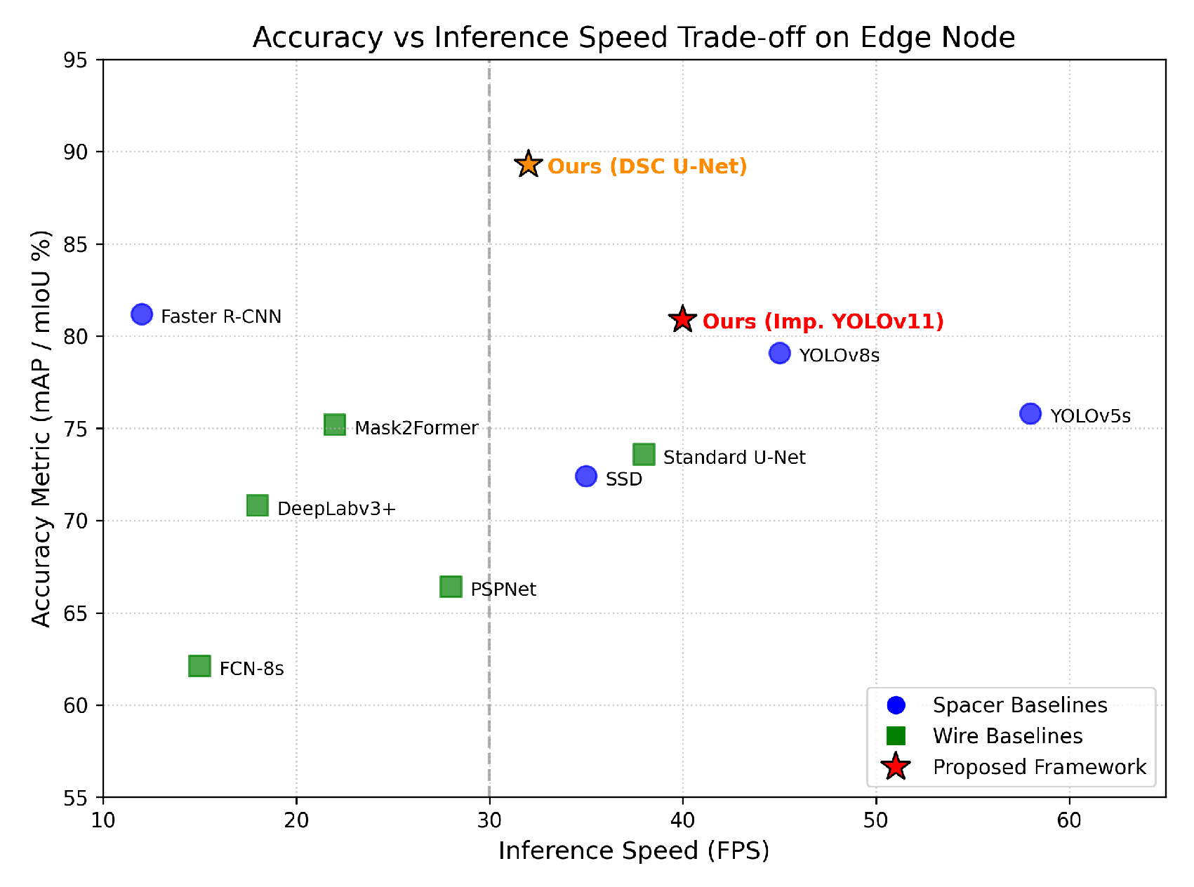
As shown, two-stage models (Faster R-CNN) and Transformer-based models (RT-DETR, Mask2Former) achieve competitive accuracy but incur excessive GFLOPs and VRAM usage, failing the >30 FPS real-time threshold on the Jetson AGX Xavier. The proposed dual-branch framework provides a favorable tradeoff between accuracy and deployment efficiency.

Figure 3 visualizes this accuracy–speed tradeoff on the edge node.

4.3.5. Supplementary Validation on a Public Real Power-Line Dataset

To address the concern that synthetic data alone cannot demonstrate field generalization, the bare-conductor segmentation branch was additionally evaluated on an independent public real power-line dataset. The model used the same preprocessing and inference settings as in the field-video experiments. Because this dataset contains 2D image annotations but no synchronized binocular depth ground truth, the evaluation focuses on conductor extraction rather than 3D displacement reconstruction.

The results in

Table 7. Segmentation Performance on the Public Power-Line Dataset.

Dataset	Dice	IoU	Accuracy	Precision	Recall
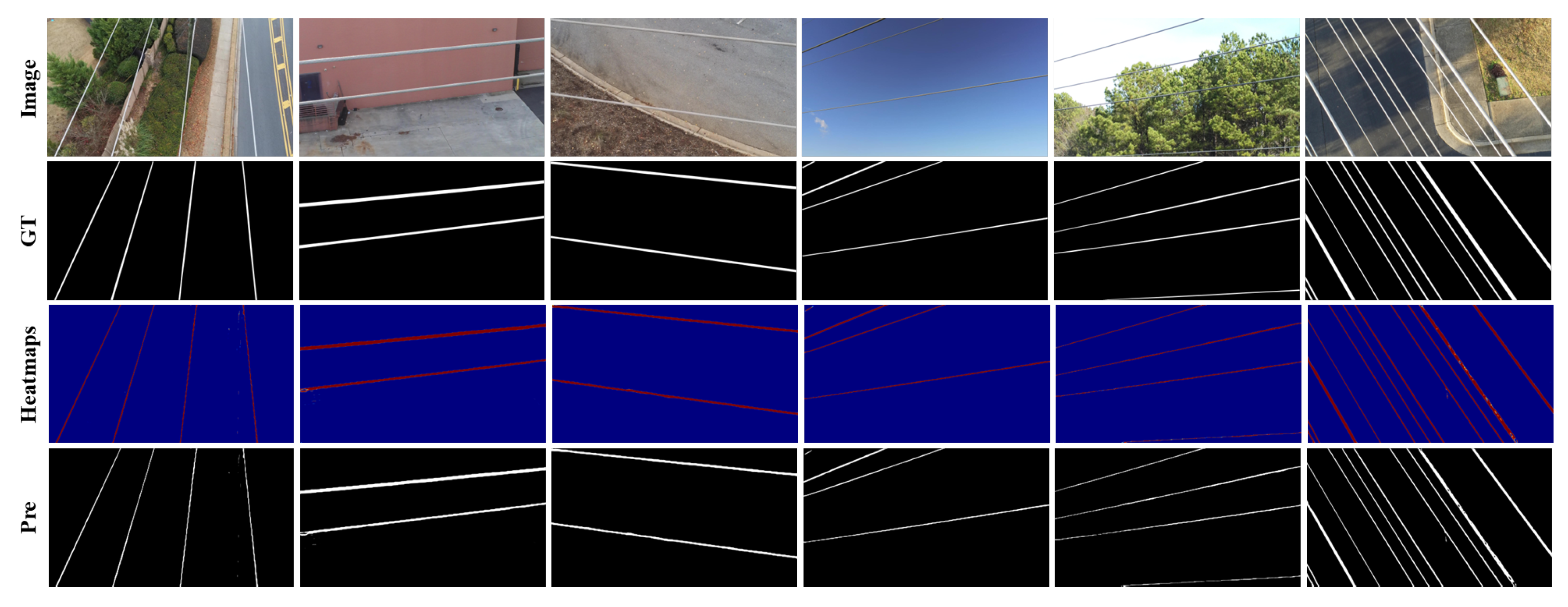
Public powerline dataset	0.9039	0.8395	0.9917	0.9693	0.8577

show that the segmentation branch maintains high precision on real images outside the self-built dataset. The relatively lower recall compared with precision indicates that the model remains conservative near weak or partially occluded line pixels. This is acceptable for avoiding false line detections in 3D reconstruction, but it also reveals a limitation: very faint line segments may still require either stronger temporal aggregation or additional real-scene annotation in future work.

Figure 4 provides qualitative examples of the public dataset evaluation.

4.4. Validation of Galloping Trajectory Reconstruction and Temporal Measurement Accuracy

4.4.1. Dynamic Ranging Accuracy

Table 8. Accuracy Comparison of 3D Spatial Ranging for Different Line Sections. Bold values indicate the best performance in each line section.

Measurement Scheme	Section Type	X-Axis RMSE (mm)	Y-Axis RMSE (mm)	Z-Axis RMSE (mm)
Monocular Estimation	Spacer	18.4	22.1	145.6
Monocular Estimation	Bare Conductor	25.3	28.7	178.2
Binocular (Ours)	Spacer	8.2	11.5	24.5
Binocular (Ours)	Bare Conductor	12.4	14.6	31.2

contrasts monocular vision constraints against our binocular collaborative measurement. The “Monocular Estimation” baseline was implemented by utilizing the Perspective-n-Point (PnP) algorithm, heavily relying on the known geometric prior of the spacer dimensions and standard conductor diameters to deduce depth.

The monocular baseline produces large Z-axis errors (RMSE greater than 140 mm) because the visual scale of a slender wire changes only weakly during out-of-plane motion. Under the controlled field-test setup, binocular disparity fusion reduces the spacer-section Z-axis RMSE to 24.5 mm and the bare-conductor Z-axis RMSE to 31.2 mm. These results show that stereo geometry substantially reduces, rather than universally eliminates, the depth-scale ambiguity of monocular measurement. Because the full target-depth distribution and pixel angular spacing were not retained in the original field log, the results should be interpreted as an empirical accuracy evaluation for the tested field sequences rather than as a complete analytical depth-accuracy model for every operating distance.

4.4.2. Temporal Consistency and Trajectory Smoothing

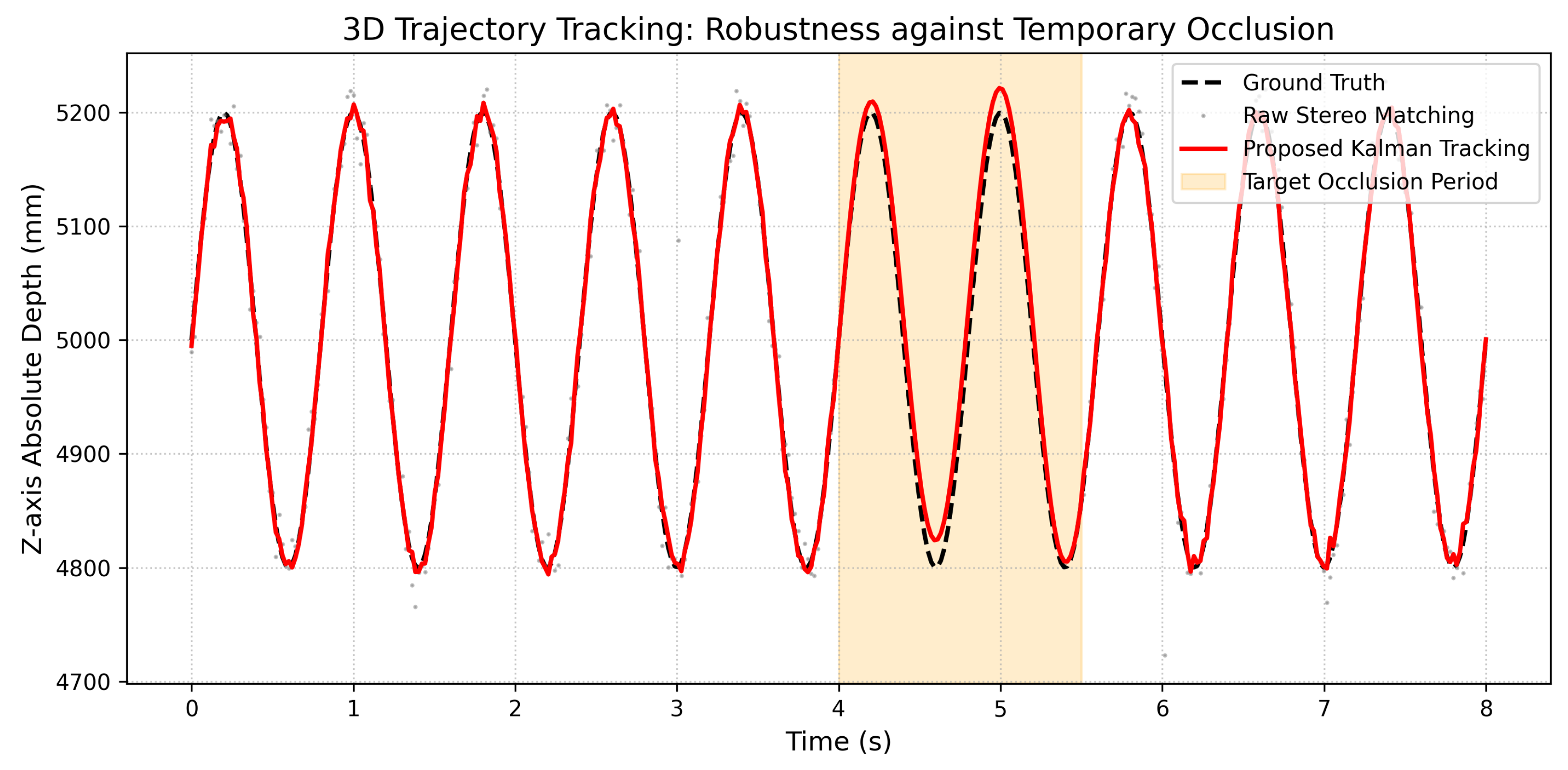
To address temporal fragmentation caused by airborne jitter or brief occlusion by moving vegetation, the cross-frame Kalman filtering acts as a critical stabilizer. Figure 5 maps the Z-axis depth tracking trajectory over time.

During continuous wind-induced galloping, raw stereo matching exhibits high-frequency noise and disparity dropouts when brief occlusions occur between $t=4.0$ s and $t=5.5$ s. By integrating the Kalman kinematic model, the system yields a smoother trajectory that remains close to the ground-truth trend during the short occlusion interval.

4.4.3. Comprehensive Test System and Dynamic Parameter Fitting Analysis

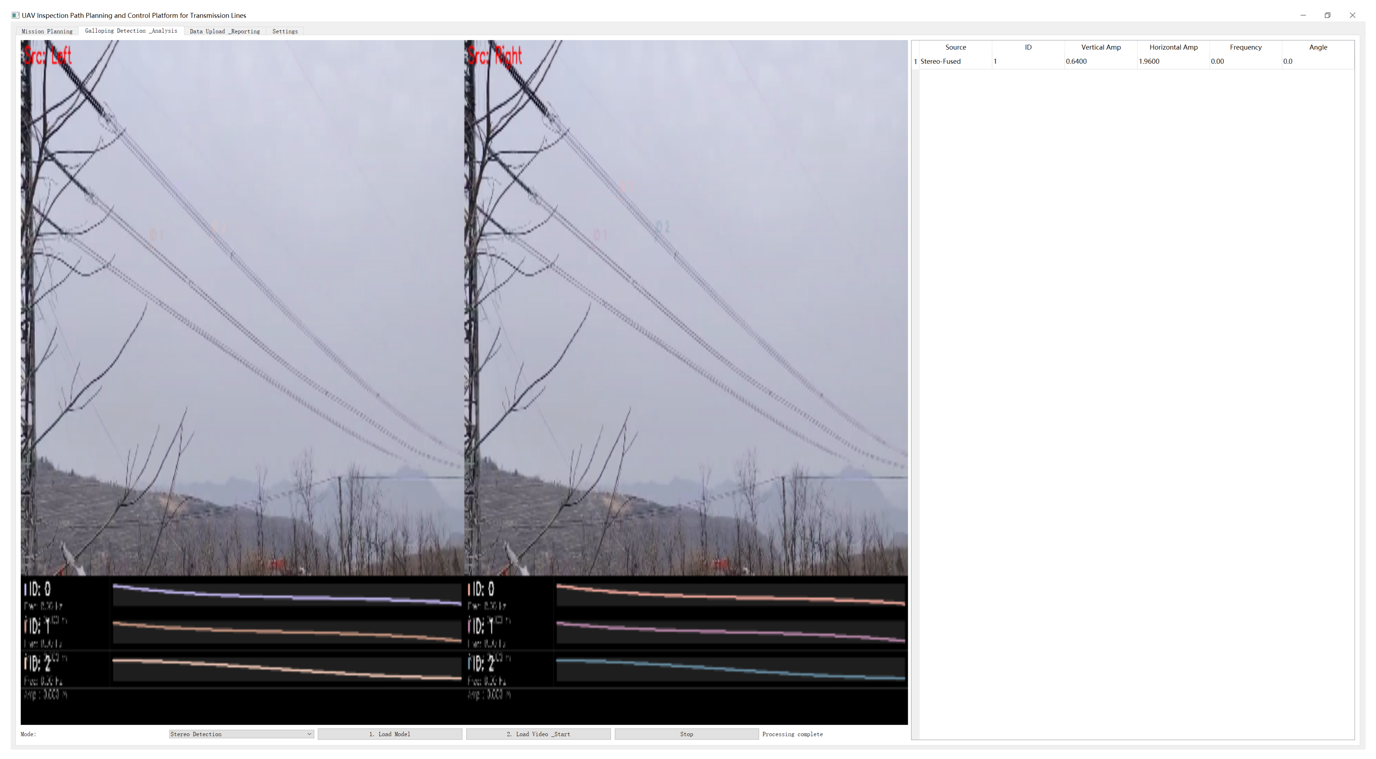
When field binocular test videos are input, the real-time operational interface of the system is shown in Figure 6. The interface synchronously displays the original video stream overlaid with feature extraction results (YOLO bounding boxes and U-Net skeletons). The reported edge-end speed of 32 FPS is measured at the test resolution used in the experiments and includes adaptive preprocessing, visual extraction, stereo projection, Kalman filtering, and dynamic-parameter calculation. GPU utilization and energy consumption were not recorded in the available deployment log; therefore, the real-time claim is limited to the measured end-to-end throughput on Jetson AGX Xavier. The system outputs dominant galloping frequency and spatial galloping amplitudes in real time; in the controlled field test, the dominant frequency was 1.25 Hz with a relative error below 3.5%.

4.4.4. Robustness Boundaries and Failure Case Analysis

No visual monitoring system is universally infallible. Through extensive field testing, this study identified three extreme corner cases (Failure Cases) where the proposed framework experiences accuracy degradation or complete tracking loss: (1) Severe Ice Coating Altering Topology: When conductors undergo extreme asymmetric ice accretion, their topological geometry changes from slender tubes to irregular clumps. This breaches the DSC operator’s structural priors, causing mIoU to drop below 40%. (2) Direct Sunglare and Lens Flare: When the UAV camera faces the sun at specific low angles, severe lens flare washes out all local gradients. Although Retinex enhancement recovers partial contrast, the stereo matching cost volume becomes completely flat, resulting in Z-axis tracking loss. (3) Camouflage in Dense Vegetation: In specific seasons, the oxidized surface color of old conductors perfectly matches the spectral signature of dense background deciduous forests. In such zero-contrast scenarios, the U-Net branch occasionally suffers from trajectory disconnection. Acknowledging these boundaries provides clear directions for future integration with multi-modal sensors (such as LiDAR or Thermal Imaging) to ensure all-weather reliability.

5. Discussion

5.1. Interpretation of Results and Working Hypotheses

The primary working hypothesis of this study was that the dynamic displacement of textureless, slender transmission lines in complex meteorological environments could be quantified more reliably by decoupling the visual extraction of rigid and flexible components, and by fusing binocular spatial data with temporal kinematic models. The experimental results support this hypothesis within the tested scenarios. By employing the proposed dual-branch architecture, the system achieved spacer detection precision of 61.3% in mAP@0.5:0.95 and bare-conductor segmentation accuracy of 89.3% in mIoU on the self-built test set, while maintaining 32 FPS on edge hardware. The public real power-line dataset further indicates that the segmentation branch generalizes to independent real images, with a Dice coefficient of 0.9039 and an IoU of 0.8395. Furthermore, the controlled binocular field test reduced the spacer-section Z-axis RMSE to 24.5 mm, demonstrating a clear advantage over the monocular baseline in the tested depth range.

5.2. Comparisons with Previous Studies

From the perspective of visual feature extraction, traditional techniques relying on gradient operators (e.g., Canny, Hough transform) [8,27] or Digital Image Correlation (DIC) [29] are vulnerable to low-contrast and textureless surfaces. While recent deep learning applications in power grid inspection have largely relied on bounding box regression (e.g., Faster R-CNN, standard YOLO) [10,30], these approaches are geometrically inefficient for slender conductors because they include excessive background pixels [32]. The proposed dual-branch strategy addresses this issue by using different representations for different structures: improved YOLOv11 keypoints for rigid spacers and DSC U-Net masks/skeletons [19,21] for flexible bare conductors.

In the context of Structural Health Monitoring (SHM), many vision-based vibration measurement technologies still rely on monocular 2D planar estimation [5,6]. Monocular methods are weak at capturing out-of-plane galloping motions because depth is not directly observed, as reflected by the large Z-axis RMSE in our baseline comparisons. Although stereo vision can recover depth, matching textureless conductors against complex sky backgrounds often leads to disparity discontinuities [44]. The integration of the Kalman filter with a constant velocity kinematic model in this study provides a spatiotemporal constraint that bridges short disparity holes and improves trajectory smoothness compared with isolated frame-by-frame stereo matching.

5.3. Broad Implications

The findings of this study have implications for the operation and maintenance of smart grids. By reducing the need for contact sensors in some monitoring scenarios [5], the proposed non-contact visual framework can provide dynamic parameters such as dominant frequency and 3D amplitude from field video. These parameters can support digital-twin modeling of transmission corridors, fatigue assessment of hardware, validation of wind-resistant designs, and early warning of galloping-induced risks.

5.4. Limitations and Future Research Directions

Despite the encouraging results, the current framework has several limitations. First, the structural priors relied upon by the DSC U-Net assume a generally tubular topology. Under extreme freezing rain or snow conditions, severe asymmetric ice accretion can change the conductor morphology into irregular clumps, reducing segmentation accuracy. Second, under direct low-angle sunglare, severe lens flare washes out local gradients, causing the stereo matching cost volume to flatten and resulting in transient tracking losses. Third, the supplementary public power-line dataset validates 2D segmentation generalization only; it does not contain synchronized binocular images or 3D ground truth for depth evaluation. Fourth, several physical acquisition metadata items requested for a complete stereo error budget, including exact field of view, pixel angular spacing, and the full depth and pixel-width distributions, were not fully retained in the available field logs. Finally, the current field tests are based on fixed or hovering camera videos, and larger-scale tests with moving platforms and more transmission corridors are still required.

Future research should focus on three aspects: (1) investigating the integration of multi-modal sensors, such as fusing binocular vision with LiDAR or thermal infrared imaging, to penetrate severe visual barriers (e.g., dense fog, absolute darkness, or severe sunglare); (2) exploring lightweight end-to-end stereo matching networks to replace the computationally heavy SGBM algorithm, further reducing the computational overhead on UAV edge nodes; and (3) expanding the dataset to include diverse ice-coated conductor morphologies to enhance the generalization capability of the segmentation models under extreme winter weather anomalies.

6. Conclusions

This paper developed a non-contact dynamic displacement measurement framework for transmission line galloping based on deep vision and binocular collaboration. By introducing adaptive image enhancement and a structure-prior-based dual-branch extraction network (improved YOLOv11 and DSC U-Net), the system localizes both rigid spacers and flexible bare conductors in field videos. The integration of binocular disparity calculation with cross-frame temporal filtering reduces the depth-scale ambiguity and short-term trajectory fragmentation observed in monocular or frame-by-frame baselines. In the controlled field tests, the system achieved a spacer-section Z-axis RMSE of 24.5 mm, a dominant-frequency relative error below 3.5%, and 32 FPS on edge hardware. The supplementary public dataset test further achieved a Dice coefficient of 0.9039 and an IoU of 0.8395 for real power-line segmentation. These results indicate that the proposed framework is a practical candidate for dynamic safety assessment and anti-galloping engineering of overhead transmission lines, while broader field validation remains necessary.