An Improved Generative Adversarial Network for Footprint Image Segmentation

Abstract

Accurate footprint image segmentation is challenging in forensic applications because fine anatomical structures, weak boundaries, and background interference can degrade segmentation performance. This study presents a task-oriented generative adversarial network (GAN)-based framework for forensic footprint image segmentation. Channel Prior Convolutional Attention (CPCA) modules are integrated into the decoder stages of the generator to recalibrate fused encoder–decoder features and preserve fine details in the toe, arch, and heel regions. In addition, a dual-branch discriminator processes image–mask pairs at the original and downsampled scales, providing complementary constraints on local boundary details and global footprint morphology. The framework is trained with a least-squares adversarial loss and a binary cross-entropy (BCE)–Dice segmentation loss. Experiments on the self-collected aFoot_2025 dataset show that the proposed framework achieves an IoU of 0.9448 and a Dice coefficient of 0.9713, outperforming the evaluated baseline and attention-based alternatives. Under the evaluated synthetic Gaussian-noise settings, the proposed method retained relatively stable segmentation performance. Furthermore, an exploratory footprint-based height-prediction analysis showed modestly lower prediction errors than the baseline GAN. These findings indicate that, under the controlled acquisition conditions of the aFoot_2025 dataset, CPCA-based feature calibration and dual-scale discrimination may improve segmentation-mask quality and provide a possible benefit for subsequent anthropometric analysis.

1. Introduction

In forensic science, biometric identification, and anthropological research, the extraction and analysis of physical evidence play a crucial role in establishing suspect identities and reconstructing crime scenes. Among various traces left at crime scenes, footprints stand out as one of the most common forms of physical evidence [1]. As a fundamental human biological characteristic, footprint morphology may remain relatively stable over time and can provide discriminative information. Whether representing two-dimensional impressions from bare feet, three-dimensional impressions, or shoe prints containing sole texture features, they contain rich morphological and biomechanical information. Traditional footprint analysis primarily relies on experienced experts conducting manual measurements and morphological comparisons [1]. However, practical forensic applications face significant challenges due to complex collection environments. These adverse factors significantly hinder the extraction of high-contrast and complete footprint features. Moreover, manual analysis consumes substantial time and labor resources [2] and is susceptible to subjective judgment biases, thereby limiting its credibility in modern forensic investigations [3]. Therefore, computer-vision methods for high-precision footprint image segmentation, accurate region extraction, and background-noise suppression are needed to support automated footprint recognition.

Footprint image segmentation serves as the foundation for subsequent morphological feature extraction, suspect profiling, and identity matching. Consequently, segmentation accuracy can strongly influence the performance of an automated identification system. Early footprint processing methods primarily relied on traditional image processing techniques or manual feature-based region extraction, such as using convex hull and defect point recognition algorithms to identify regions of interest (ROIs) like toe tips and lateral heel points [2]. Regarding anthropometric feature inference, Wicaksono et al. [4] utilized Gabor wavelet features combined with the k-nearest neighbors (k-NN) algorithm to achieve automatic measurement of height and weight. Garcia-Mora et al.’s systematic review [3] also demonstrated significant statistical correlations between physical measurements obtained via traditional inked footprint methods, foot contour analysis, and pedigraphs and individual height. However, these conventional approaches are highly susceptible to noise and environmental variations. They often exhibit poor robustness when processing complex footprint images, particularly those with blurred boundaries or low contrast.

In recent years, with the rapid advancement of deep learning technologies, significant progress has been made in footprint analysis and recognition methods based on discriminative deep models. In identity matching and recognition tasks, Abuqadumah et al. [5] demonstrated the feasibility of transfer learning for small-sample footprint recognition by fine-tuning five classical models including Inception v3. Jang et al. [6] developed the Shoe-MS algorithm that effectively enhances the objectivity of shoeprint comparison through deep learning. To meet the real-time requirements of portable forensic evidence devices, Shen et al. [7] proposed a lightweight YOLOv8-StarNet detection method with low computational complexity. Meanwhile, in the field of footprint multimodal development, Zhou Xudong et al. [8] recently established a large-scale, standardized multimodal footprint dataset encompassing single-pressure impressions, sequential pressure patterns, and optical features. They introduced a Spatiotemporal Prompt Transformer (STPT) baseline model that successfully captures often-overlooked dynamic pressure sequence characteristics, providing robust data and technical support for footprint deep modeling.

Although existing research has made progress in the fields of footprint recognition and image segmentation, several technical limitations remain: First, footprint image segmentation differs substantially from conventional semantic segmentation tasks due to its unique forensic and biometric characteristics. Unlike natural objects, footprint images contain fine-grained anatomical structures, such as toe boundaries, arch regions, and heel pressure areas. These structures often exhibit significant local intensity variations and weak edge continuity. In forensic applications, these subtle structural details are directly related to downstream tasks such as identity recognition, gait analysis, and stature estimation. Therefore, footprint segmentation requires not only accurate foreground extraction but also preservation of anatomical geometry and local structural continuity. Second, there is a lack of network structure optimization for the footprint segmentation task. The standard segmentation network has limited ability to capture the details of key anatomical sites such as the toes, heel, and heavy-pressure areas. Meanwhile, as traditional noise suppression methods have limitations in adapting to complex noise environments, it is difficult for the standard segmentation network to effectively suppress the interference of background noise, while deep learning-based noise suppression technologies have shown remarkable progress in improving noise suppression effects in related fields.

While footprint image segmentation is a fundamental task, its ultimate significance lies in enabling downstream forensic applications, particularly biometric height estimation. Accurate height prediction demands highly precise extraction of anatomical landmarks and geometric contours. Therefore, this study aims to develop a segmentation framework that generates high-fidelity binary masks for footprint images acquired under the evaluated conditions. The downstream height-prediction experiment is included as an exploratory analysis to examine whether improved segmentation masks may benefit subsequent morphological feature extraction, rather than to establish operationally reliable stature estimation from forensic evidence. The contributions of this study are summarized as follows: (1) A GAN-based segmentation framework is adapted for forensic footprint images, where fine anatomical structures, weak boundaries, and background interference make accurate mask generation challenging. (2) CPCA modules are integrated into the decoder stages of the generator to recalibrate fused encoder–decoder features and improve the preservation of fine details in the toe, arch, and heel regions. (3) A dual-branch discriminator operating at two input scales is employed to evaluate image–mask pairs at the original and downsampled resolutions, providing complementary constraints on local boundary details and global footprint morphology. (4) Robustness experiments and an exploratory downstream footprint-based height-prediction analysis are conducted to assess the stability of the proposed framework and to examine whether improved segmentation masks may provide potential benefits for subsequent footprint analysis. The downstream results are interpreted as preliminary evidence rather than definitive proof of a substantial forensic advantage.

The remainder of this paper is organized as follows. Section 2 reviews the related work. Section 3 describes the proposed GAN-based footprint segmentation method, including the network architecture and optimization strategy. Section 4 presents the experimental setup, comparative studies, ablation analyses, and robustness evaluations. Finally, Section 5 concludes the paper and outlines future work.

2. Related Work

2.1. GAN-Based Segmentation Methods

Generative adversarial networks (GANs) were first proposed by Goodfellow et al. as an adversarial learning framework in which a generator and a discriminator jointly model data distributions [9]. Through adversarial training, the generator progressively produces samples closer to the true distribution, while the discriminator continuously enhances its ability to distinguish between real and generated samples. Although classical GANs achieved significant breakthroughs in image generation tasks, their training process suffers from issues such as instability, vanishing gradients, and mode collapse. To improve training performance, Least Squares GAN (LSGAN) introduces a least squares loss function, thereby enhancing training stability, visual quality of generated samples, and convergence speed [10].

The Conditional Generative Adversarial Network (cGAN) enables controlled generation by incorporating conditional information derived from input images or structural features [11]. The pix2pix model is a representative method in this field, using a U-Net generator and PatchGAN discriminator to achieve end-to-end image-to-label mapping [11]. In semantic segmentation tasks, GANs not only rely on pixel-level supervision signals but also impose distribution-based constraints on predictions, thereby enhancing structural consistency and boundary clarity. Luc et al. [12] were among the first to apply adversarial learning to semantic segmentation, improving spatial structural consistency. Hoffman et al. further utilized GANs for domain adaptation in fully convolutional networks (FCNs), achieving pixel-level feature alignment across diverse scenarios and enhancing the model’s generalization performance in complex environments [13]. Furthermore, Kozinski et al. proposed introducing an adversarial regularization mechanism into structured output networks to simultaneously optimize both output distribution and structural consistency during model training [14]. Souly et al., on the other hand, investigated the application of GANs in semi-supervised and weakly supervised semantic segmentation, leveraging generators to enhance learning performance under conditions of limited labeled data [15]. These studies suggest that a key advantage of GANs in semantic segmentation lies in their ability to incorporate distribution-level constraint mechanisms, thereby significantly enhancing the overall quality of structural prediction tasks.

2.2. Multi-Scale Discrimination Mechanism

Multi-scale GANs improve modeling capacity in complex scenarios by constructing discriminative paths at different resolutions, enabling simultaneous capture of global structure and local details [16]. Zang et al. proposed a method combining multi-scale CBAM with dual-branch GANs to improve structural representation in early-stage CT image detection [17]. Al-Khazraji et al. further developed a multi-scale dual-discriminator GAN for gas leakage detection, enhancing model robustness in complex environments through scale-specific discriminative pathways [18]. Cheng et al. introduced the MS-STGAN framework, achieving efficient representation of complex time-series data via multi-scale structural modeling [16]. Nguyen et al. pioneered the Dual Discriminator GAN, where two independent discriminators constrain distinct feature distributions to improve generation quality and training stability [19]. Wang et al. proposed a dual-channel fusion-based dual-discriminator GAN for infrared-visible image fusion, effectively strengthening cross-modal structural consistency [20]. Zhao et al. further proposed a dual-branch GAN for image de-raining tasks, where distinct branches model structural information and noise distributions, respectively, thereby enhancing image restoration performance under complex weather conditions [21]. Overall, multi-scale and multi-branch discriminative mechanisms significantly enhance GANs’ ability to model complex structures and improve training stability.

2.3. Attention Mechanisms

In deep learning-based image segmentation, attention mechanisms are widely used to enhance a model’s ability to capture key features. Channel and spatial attention mechanisms have evolved to improve a network’s adaptive representation of informative features. Squeeze-and-Excitation Networks (SENet) achieve adaptive recalibration of feature channels by explicitly modeling inter-channel dependencies, thereby substantially improving the expressive power of convolutional networks [22]. Building on this foundation, Efficient Channel Attention (ECA) further optimizes channel attention mechanisms through a local cross-channel interaction strategy, effectively reducing model complexity while avoiding dimensionality reduction, thus enabling lightweight yet efficient modeling [23]. Meanwhile, Convolutional Block Attention Module (CBAM) sequentially introduces attention mechanisms across both channel and spatial dimensions, achieving dual feature enhancement that improves network responsiveness to key regions and demonstrates consistent performance improvements across various visual tasks [24]. Additionally, Channel Prior Convolutional Attention Mechanism (CPCA) integrates channel prior modeling with multi-scale depthwise convolutions to enable dynamic attention allocation across the channels and spatial dimensions, significantly enhancing the model’s focus on important channels and critical spatial regions [25]. CPCA is particularly relevant to our framework because it provides effective prior-guided feature enhancement, which is essential for fine-grained footprint structure modeling. Overall, attention mechanisms have evolved from channel-only modeling (SE, ECA) to channel-spatial joint modeling (CBAM), and further to prior-guided multi-scale adaptive attention (CPCA). This evolution improves feature representation in complex segmentation tasks.

3. Methods

Recent adversarial generative frameworks based on GANs have received substantial attention in image analysis [26,27,28,29]. Their ability to model data distributions and generate high-fidelity outputs makes GANs useful for image-segmentation tasks [30]. However, CNN-based generators used in most GAN architectures suffer from an inherent limitation. As network depth increases, local spatial information gradually diminishes, and deeper features become dominated by global semantic representations. Although skip connections are commonly employed to mitigate local information loss, traditional skip connections typically rely solely on direct concatenation or simple addition of shallow and deep features, lacking selective fusion across layers. This straightforward fusion strategy may introduce redundant information and unnecessary noise, potentially compromising the generator’s representation capacity and adversely affecting overall generation performance.

3.1. Generative Adversarial Network

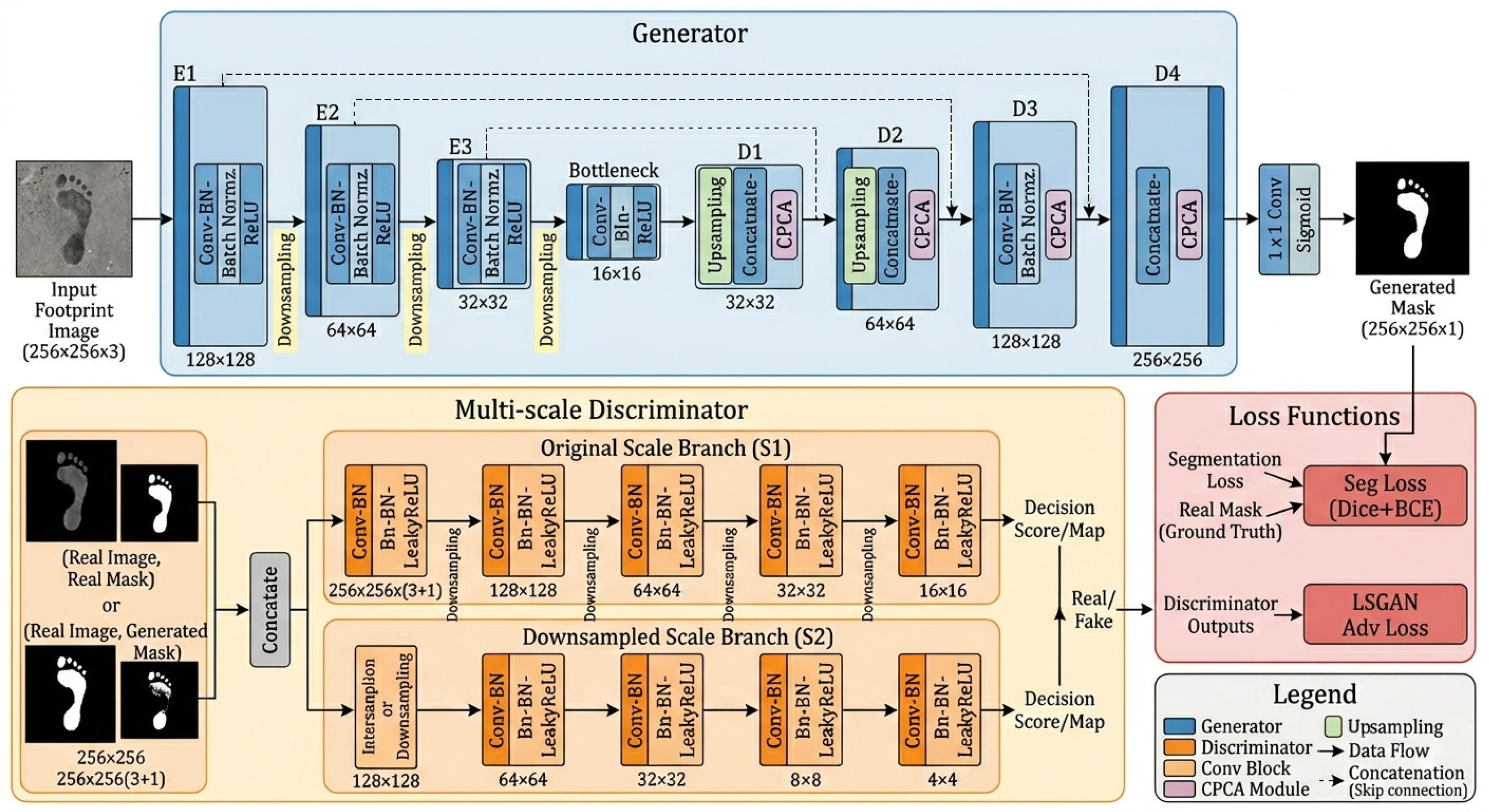
The proposed footprint image segmentation approach is based on a generative adversarial network. The generator produces binary segmentation masks from the original footprint image, whereas the discriminator distinguishes generated masks from ground-truth masks, as illustrated in Figure 1. The proposed framework integrates the CPCA module into the generator and employs a multi-scale discriminator. These designs are intended to improve footprint segmentation quality in the evaluated image-acquisition setting by enhancing the representation of boundary details and footprint morphology. CPCA enables the dynamic allocation of attention weights across the channel and spatial dimensions. This mechanism allows the model to focus on informative feature channels and critical spatial regions. Meanwhile, channel prior information is preserved during feature extraction. As a result, it enhances feature representation capability.

Following conditional GAN-based image-to-image translation methods, footprint segmentation is formulated as a mapping from an input footprint image x to a binary mask y [11]. To improve adversarial training stability, the least-squares adversarial objective proposed in LSGAN is adopted [10]. The discriminator evaluates whether an image–mask pair is real or generated. The detailed adversarial losses are provided in Section 3.4.1.

3.2. Generator Network Design

The generator follows the encoder–decoder architecture of U-Net [31]. CPCA modules are inserted at each decoder stage to recalibrate the fused encoder–decoder features [25]. Unlike standard U-Net architectures that rely solely on skip connections for feature fusion, this design enhances the network’s ability to focus on critical footprint regions such as toes and heels, while suppressing interference from the background and irrelevant textures. This improves the generator’s ability to reconstruct detailed footprint structures.

3.2.1. Feature Fusion

$F_e\in {ℝ}^{C\times H\times W}$ denotes the high-resolution feature map output by the encoder. $F_d\in {ℝ}^{C\times H\times W}$ denotes the feature map obtained after upsampling at the next level of the decoder.

First, channel concatenation and dimensionality reduction are performed.

$$F_{\mathrm{fuse}}={\mathrm{Conv}}_{1\times 1}\left(\mathrm{Concat}(F_e,F_d)\right)\in {ℝ}^{C\times H\times W}$$

(1)

where $\mathrm{Concat}(\cdot )$ represents channel concatenation, $Con{v}_{1\times 1}$ restores the number of channels to C.

3.2.2. CPCA Module

The Channel Prior Convolutional Attention (CPCA) mechanism was originally introduced to jointly model channel priors and multi-scale spatial information [25]. In this study, CPCA is integrated into the decoder stages of the generator for forensic footprint segmentation.

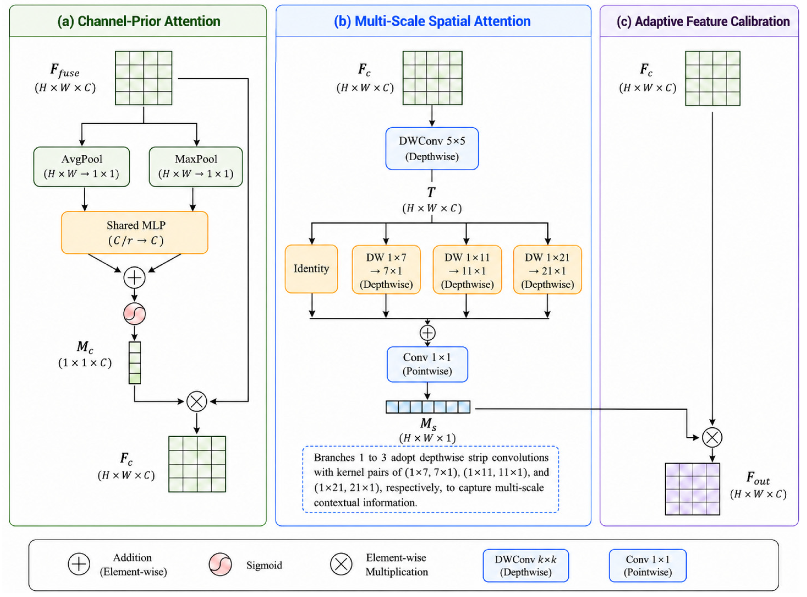
The CPCA module is designed to enhance feature representation by combining channel-level priors with multi-scale spatial information. As illustrated in Figure 2, the CPCA module consists of three sequential stages: channel-prior attention, multi-scale spatial attention, and adaptive feature calibration. The channel-prior attention stage generates channel-wise weights from global average-pooled and max-pooled descriptors. The resulting channel-attention map is multiplied by the fused feature map to obtain the channel-prior feature representation. The multi-scale spatial-attention stage then extracts local and long-range spatial information using an initial depthwise convolution and parallel depthwise strip-convolution branches. Finally, the spatial-attention map is multiplied by the channel-prior feature map to obtain the refined output feature.

(1)

Channel Prior Weight Calculation

Given the feature map $F_{fuse}$, CPCA computes inter-channel correlations to generate a prior distribution. First, global average pooling and global max pooling reduce the spatial dimensions. A shared multilayer perceptron (MLP) is used to capture dependencies between channels

$$z=MLP(\mathrm{GAP}(F_{fuse}))+MLP(\mathrm{GMP}(F_{fuse}))$$

(2)

Then, channel prior weights are generated using the sigmoid function.

$$M_C=\sigma \left(z\right)\in {ℝ}^C$$

(3)

where $\sigma$ denotes the sigmoid activation function. The weights $M_C$ quantify the contribution of different feature channels to the footprint feature representation.

(2)

Multi-scale Spatial Representation Extraction

The intermediate feature map $F$ is processed through a series of convolutions to extract multi-scale spatial representations. The resulting feature map is processed by four parallel branches. Branch 0 is an identity connection, whereas Branches 1–3 use depthwise strip convolutions. Let the convolution kernel size of the i-th parallel branch be $k_i$, then the output feature is

$$S_i={\mathrm{DWConv}}_{k_i}(F)$$

(4)

The branch outputs are fused by element-wise summation and subsequently processed by a $1\times 1$ convolution for channel mixing.

$$M_S={\mathrm{Conv}}_{1\times 1}\left({\displaystyle \sum _{i=0}^3{S}_i}\right)$$

(5)

This design enlarges the receptive field without introducing substantial computational overhead [25]. As a result, the module can effectively capture the overall footprint contour. As shown in

Table 1. Detailed configuration of the CPCA module.

Stage	Operator	Kernel	Output
Input	Fused feature map	—	H × W × C
Channel attention	AvgPool + MaxPool + shared MLP	—	1 × 1 × C
Channel prior	Element-wise multiplication	—	H × W × C
Initial feature extraction	DWConv	5 × 5	H × W × C
Branch 0	Identity	—	H × W × C
Branch 1	Strip DWConv	1 × 7, 7 × 1	H × W × C
Branch 2	Strip DWConv	1 × 11, 11 × 1	H × W × C
Branch 3	Strip DWConv	1 × 21, 21 × 1	H × W × C
Fusion	Element-wise summation	—	H × W × C
Channel mixing	Conv	1 × 1	H × W × C
Output	Element-wise multiplication	—	H × W × C

Notes: “—” indicates that this item is not applicable.

, the module employs four parallel depthwise convolution branches: An initial 5 × 5 depthwise convolution is first applied to extract local spatial information. The resulting feature map is then processed by four parallel branches, including an identity branch and three depthwise strip-convolution branches. Branches 1–3 adopt depthwise strip convolutions with kernel pairs of (1 × 7, 7 × 1), (1 × 11, 11 × 1), and (1 × 21, 21 × 1), respectively, to capture multi-scale contextual information. All depthwise convolutions preserve the channel dimension C and preserve spatial resolution through appropriate padding. The outputs of the four branches are fused by element-wise summation, and then passed through a 1 × 1 convolution to generate a spatial attention map.

(3)

Adaptive Feature Calibration

The channel prior weights $M_C$ are combined with the feature F to produce an intermediate feature map $F_c$

$$F_c=M_C\odot F$$

(6)

The operation $\odot$ performs element-wise multiplication.

Then, $F_c$ is multiplied element-wise with $M_S$ to obtain the final feature map.

$$F_{\mathrm{out}}=M_S\odot F_c$$

(7)

The final output feature map $F_{\mathrm{out}}$ not only enhances the edge features of the footprint in the spatial dimension but also suppresses redundant background responses in the channel dimension.

3.2.3. Forward Propagation of the Generator

The calibrated feature map $F_{\mathrm{out}}$ is passed to the subsequent decoder convolutional layer. The final output layer uses a 1 × 1 convolution followed by a sigmoid activation function to produce a pixel-level segmentation probability map:

$$\widehat{y}=\sigma \left({\mathrm{Conv}}_{1\times 1}(F_{\mathrm{dec}}^{(L)})\right)\in {[0,1]}^{H\times W}$$

(8)

where $F_{\mathrm{dec}}^{(L)}$ is the feature map output by the final decoder layer.

3.3. Discriminator Network Design

Multi-scale adversarial discrimination has been used to capture structural information at different resolutions [26]. Building on this idea, this study employs a dual-branch discriminator that processes image–mask pairs at the original and downsampled scales. The discriminator employs a multi-scale architecture to extract local and global features, including edges, textures, and region-level structures, at various scales, thereby enhancing robustness and reducing noise interference.

We design a dual-branch, multi-scale discriminator D. The original-scale branch directly processes image–mask pairs at the original resolution. This branch focuses on evaluating edge consistency and local texture realism. The downsampling branch applies 2× downsampling to the input pairs. It is designed to capture global geometric structures and anatomical features.

Each discriminator branch contains six convolutional layers, as summarized in

Table 2. Layer-wise configuration of each branch in the dual-scale discriminator.

Layer	Layer Type	Kernel	Stride	Padding	Input Channels	Output Channels	Normalization	Activation
1	Conv2D	4 × 4	2	1	4	64	—	LeakyReLU (0.2)
2	Conv2D	4 × 4	2	1	64	128	BN	LeakyReLU (0.2)
3	Conv2D	4 × 4	2	1	128	256	BN	LeakyReLU (0.2)
4	Conv2D	4 × 4	2	1	256	512	BN	LeakyReLU (0.2)
5	Conv2D	4 × 4	2	1	512	512	BN	LeakyReLU (0.2)
6	Conv2D	4 × 4	1	1	512	1	—	—

Notes: The input channel number is 4 (3-channel RGB image + 1-channel mask); BN denotes Batch Normalization. The final layer has no activation function and directly outputs logits for the LSGAN mean-squared-error (MSE) loss. The two branches share identical structures but have independent parameters and do not share weights; “—” indicates that this item is not applicable.

. The discriminator input is formed by concatenating a three-channel RGB footprint image and a one-channel segmentation mask, resulting in a four-channel input. The original-scale branch processes the original image–mask pair, whereas the downsampled-scale branch processes the corresponding pair after 2× downsampling. The two branches have identical layer configurations but independent parameters.

Each branch produces a PatchGAN score map rather than a single scalar output. The two branches have identical architectures but independent parameters, and no feature-level fusion is performed between them. Their branch-specific adversarial losses are calculated independently and then combined through weighted loss aggregation, as described in Section 3.4.1.

The branch-weighting coefficient α was selected using a validation-set parameter sweep over {0.1, 0.3, 0.5, 0.7, 0.9}. All other experimental settings were kept unchanged. Validation IoU was used as the primary criterion for selection. The highest validation IoU was obtained at $\alpha$ = 0.5; therefore, equal loss weights were assigned to the two branches in all subsequent experiments. The held-out test set was not used for parameter selection.

High-level features have larger receptive fields and stronger semantic abstraction but lower spatial resolution. A larger receptive field means each neuron can access a wider range of the original image, implying it may contain more global and higher-level semantic features. The high-level network has strong global geometric information representation capabilities, and the low-level network has a small receptive field and strong geometric detail information representation capabilities. As mentioned in relevant research, the multi-scale design can expand the discriminator’s perception range, improving its ability to capture image details, reduce artifacts in generated images and correct errors. This allows the discriminator to concurrently focus on global structural consistency and local edge details, which in turn guides the generator to generate more realistic and continuous segmentation results. This aligns with the application logic of multi-scale feature fusion in image segmentation, which has been verified by experiments to effectively improve the accuracy of image segmentation, and has been widely applied in fields such as medical image segmentation.

3.4. Loss Functions

The overall training objective of the proposed framework comprises two distinct types of loss functions, each serving a specific purpose in the adversarial learning process. The first is the adversarial loss, which governs the competition between the generator and the discriminator, ensuring that the generated segmentation masks progressively become indistinguishable from the ground-truth labels. The second is the segmentation loss, which directly supervises the generator’s output at the pixel level, enforcing classification accuracy and structural consistency with the target masks.

3.4.1. Least-Squares Adversarial Loss

To alleviate gradient vanishing and training instability in standard GAN training, this paper adopts Least-Squares GAN (LSGAN) as the optimization target. Unlike the sigmoid cross-entropy loss used in standard GANs, which tends to saturate and cause gradient vanishing during training, LSGAN uses mean squared error (MSE) as the loss function. This loss penalizes generated samples that are far from the decision boundary. Therefore, the generated distribution is encouraged to better approximate the real data distribution. In addition, the loss provides more stable gradients during training, which improves convergence stability and sample quality. Let $D_1$ and $D_2$ denote the original-scale and downsampled-scale discriminator branches, respectively. Each branch independently evaluates real and generated image–mask pairs using the least-squares objective. For branch s, where $s\in \{1,2\}$, the discriminator loss is defined as:

$${\mathcal{L}}_D^{(s)}={\displaystyle \frac{1}{2}}{\mathbb{E}}_{(x,y)~p_{\mathrm{data}}}\left[{\left(D_s(x,y)-1\right)}^2\right]+{\displaystyle \frac{1}{2}}{\mathbb{E}}_{x~p_{\mathrm{data}}}\left[D_s{\left(x,G(x)\right)}^2\right],s\in \{1,2\}$$

(9)

The corresponding adversarial loss of the generator for branch s is:

$${\mathcal{L}}_{G,\mathrm{adv}}^{(s)}={\displaystyle \frac{1}{2}}{\mathbb{E}}_{x~p_{\mathrm{data}}}\left[{\left(D_s\left(x,G(x)\right)-1\right)}^2\right],s\in \{1,2\}$$

(10)

The discriminator losses from the two branches are combined as:

$${\mathcal{L}}_D=\alpha {\mathcal{L}}_D^{(1)}+(1-\alpha ){\mathcal{L}}_D^{(2)}$$

(11)

Similarly, the generator adversarial losses from the two branches are combined as:

$${\mathcal{L}}_{G,\mathrm{adv}}=\alpha {\mathcal{L}}_{G,\mathrm{adv}}^{(1)}+(1-\alpha ){\mathcal{L}}_{G,\mathrm{adv}}^{(2)}$$

(12)

Here, x denotes the input footprint image, y is the corresponding ground-truth mask, and G(x) is the predicted segmentation probability map. $D_1$ and $D_2$ denote the original-scale and downsampled-scale discriminator branches, respectively. The discriminator assigns real image–mask pairs target values close to 1 and generated image–mask pairs target values close to 0, whereas the generator encourages generated pairs to receive scores close to 1. The coefficient $\alpha \in [0,1]$ controls the relative contributions of the two discriminator branches. Based on the validation-set parameter sweep described in Section 3.3, $\alpha$ was set to 0.5 in all subsequent experiments.

3.4.2. Hybrid Segmentation Loss for Generator Supervision

While the adversarial loss guides the generator toward producing masks that are statistically consistent with the ground-truth mask distribution, it does not provide explicit spatial or categorical supervision. Therefore, we introduce a dedicated segmentation loss that directly compares the generated mask with the ground-truth annotation at the pixel level. This loss is crucial for preserving local structural details, especially in challenging regions such as toe boundaries and heel contours, where the adversarial signal alone may be insufficient or ambiguous.

The segmentation loss combines binary cross-entropy (BCE) with a Dice-based overlap term. Dice-based optimization has been widely used to mitigate foreground–background imbalance in segmentation tasks [32]. Combined cross-entropy and Dice objectives have also been used to balance pixel-wise classification and region-overlap supervision [33]. In this study, we employ a weighted BCE–Dice formulation tailored to the footprint segmentation task.

BCE loss evaluates the classification accuracy independently per pixel, providing a strong and stable gradient for every spatial position. It treats all pixels equally, which helps in reducing false positives and false negatives across the entire image.

Dice loss measures the overlap between the predicted mask and the ground truth. It is particularly effective in handling class imbalance, which is prevalent in footprint images where the foreground (foot region) often occupies a much smaller area than the background. By directly optimizing mask overlap, Dice loss penalizes missed foreground regions more strongly, thereby encouraging the generator to preserve the integrity of the foot silhouette.

The combined segmentation loss is defined as:

$${\mathcal{L}}_{G,seg}={\lambda }_{\mathrm{BCE}}\cdot {\mathcal{L}}_{\mathrm{BCE}}+{\lambda }_{\mathrm{Dice}}\cdot {\mathcal{L}}_{\mathrm{Dice}}$$

(13)

where

$${\mathcal{L}}_{\mathrm{BCE}}=-{\displaystyle \frac{1}{N}}{\displaystyle \sum _{i=1}^N\left[\begin{array}{c}{y}_i\log (p_i)+(1-y_i)\log (1-p_i)\end{array}\right]}$$

(14)

$${\mathcal{L}}_{\mathrm{Dice}}=1-{\displaystyle \frac{2{\displaystyle \sum _i{y}_i}{p}_i+ϵ}{{\displaystyle \sum _i{y}_i}+{\displaystyle \sum _i{p}_i}+ϵ}}$$

(15)

Here, $y_i$ and $p_i$ denote the ground-truth label and predicted probability at pixel i, N the total number of pixels, and $ϵ$ is a small smoothing term to avoid numerical instability. In our experiments, we set ${\lambda }_{BCE}=1.0$ and ${\lambda }_{Dice}=0.5$ to balance pixel-wise accuracy and regional overlap.

3.4.3. Overall Generator Objective

The total loss for the generator combines the adversarial loss and the segmentation loss in a weighted sum:

$${\mathcal{L}}_G={\mathcal{L}}_{G,adv}+{\lambda }_{seg}\cdot {\mathcal{L}}_{G,seg}$$

(16)

where $L_{G,adv}$ is the weighted adversarial loss aggregated from the original-scale and downsampled-scale discriminator branches, as defined in Equation (12). $L_{G,seg}$ denotes the hybrid BCE–Dice segmentation loss, and ${\lambda }_{seg}$ controls the relative contribution of segmentation supervision. During adversarial training, the two discriminator branches jointly minimize the weighted discriminator objective $L_D$. The generator minimizes the total objective ${\mathcal{L}}_G$, which consists of the weighted dual-branch adversarial loss $L_{G,adv}$ and the hybrid segmentation loss $L_{G,seg}$. Thus, the adversarial component constrains the predicted masks at both the original and downsampled scales, whereas the BCE–Dice component provides direct pixel-level and region-overlap supervision.

4. Experimental Evaluation

4.1. Experimental Setup

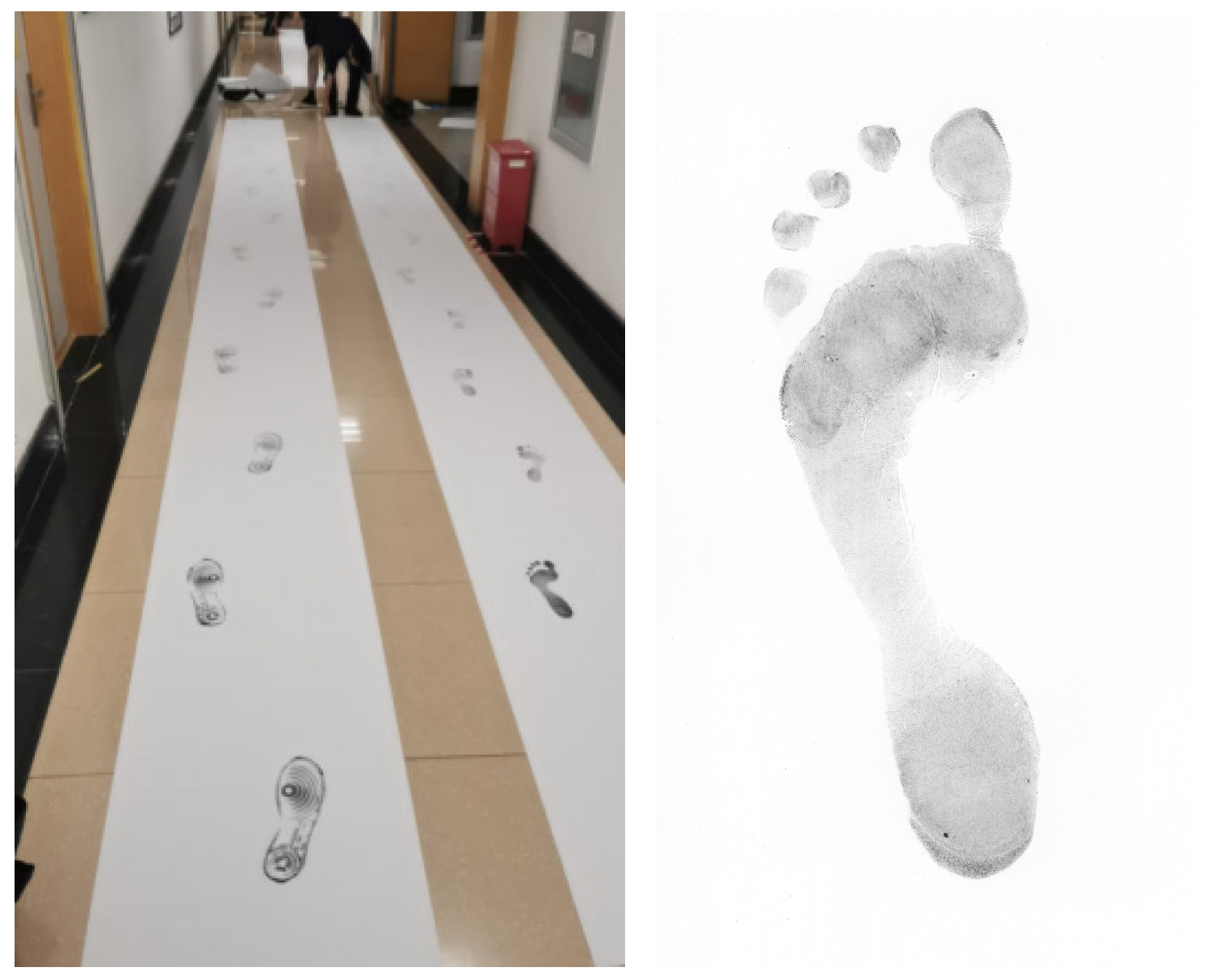
We used a self-collected aFoot_2025 footprint image dataset. Continuous-form engineering drawing paper (310 mm wide) was used as the trace-recording medium. Standardized ink was applied to the footprint plate to ensure complete coverage of the sole, supplemented by forensic scale drawings as spatial calibration references. During data acquisition, participants stood naturally on the footprint plate to ensure uniform pressure distribution. Adequate ink coverage was obtained for the arch, toe, and heel regions. Participants then walked along a 10 m paper track at a normal pace. For each collection session, only stable footprints from the middle section of the sequence were retained as shown in Figure 3. A total of 145 healthy volunteers aged 18–65 years were recruited, evenly distributed into three age groups: young adults (18–34 years), middle-aged adults (35–49 years), and older adults (50–65 years)-with balanced gender representation. Each participant provided 30 footprints. All footprints were scanned with a high-speed scanner at 300 dpi resolution to eliminate perspective distortion and lens deformation, ensuring strict linear correspondence between pixel coordinates and physical dimensions. The images were uniformly labeled according to anthropometric indicators, ultimately forming a structured dataset. In the experiment, a total of 4350 footprint images and their corresponding manually labeled binary masks were used. All images were resized to 256 × 256 pixels. To evaluate the performance of the proposed method, we used the self-collected aFoot_2025 dataset.

4.1.1. Footprint Image Annotation

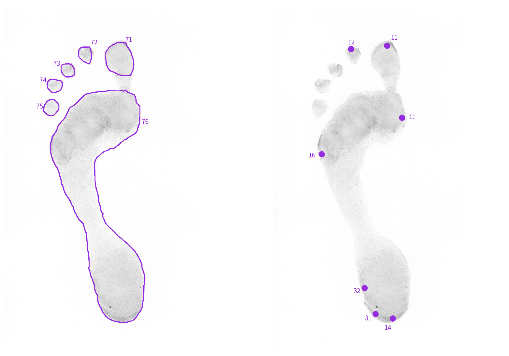
Footprint image annotation was performed manually using the X-AnyLabeling software version 3.0.3. Each annotation comprised two components: contour regions and key points. For contour annotation, the footprint was divided into six anatomical regions based on foot anatomy: the great toe (71), second toe (72), third toe (73), fourth toe (74), little toe (75), and forefoot/arch/heel region (76). Each region was delineated at the pixel level using a polygon tool. Seven anatomical landmarks were identified: great toe apex (11), second-toe apex (12), heel point (14), medial arch point (15), lateral arch point (16), footprint trace point A (31), and footprint trace point B (32), with their coordinates recorded using a point tool as shown in Figure 4. Notably, this segmentation task utilized only contour information, grouping regions 71–76 as a single foreground category and classifying the background as a separate category to achieve comprehensive footprint segmentation. All annotation results were saved in JSON format, with key point information retained for subsequent morphological analysis.

4.1.2. Model and Training Setup

The proposed framework was implemented using Python 3.9.25 and PyTorch 2.0.1. The generator followed a U-Net-style encoder–decoder architecture with base channel numbers of 32, 64, 128, and 256 in the four resolution stages. CPCA modules were inserted after the feature-fusion block at each decoder stage to recalibrate the fused encoder–decoder features. The discriminator employed a dual-branch multi-scale design. Its original-scale branch processed the input image–mask pair at the original resolution, whereas the second branch processed the corresponding pair after 2× downsampling. The two branches had identical architectures but independent parameters. Detailed configurations of the CPCA module and discriminator are provided in Table 1 and Table 2, respectively.

The aFoot_2025 dataset comprised 4350 footprint images collected from 145 participants. To prevent participant-level information leakage, the dataset was partitioned before training at the participant level rather than at the image level. Specifically, 116 participants were assigned to the training subset, 14 participants to the validation subset, and 15 participants to the independent test subset. All images from an individual participant were assigned exclusively to one subset. This participant-independent split was fixed and used consistently for all compared methods and repeated runs.

All footprint images and their corresponding binary masks were resized to 256 × 256 pixels. Images were converted to RGB, scaled to the range [0, 1], and normalized using channel-wise mean values of [0.485, 0.456, 0.406] and standard deviations of [0.229, 0.224, 0.225]. Binary masks were resized using nearest-neighbor interpolation to preserve label boundaries. Data augmentation was applied only to the training subset. The augmentation pipeline included horizontal flipping, vertical flipping, and random rotation within the range of −30° to 30°. The same geometric transformation was synchronously applied to the image and its corresponding mask. No random augmentation was applied to the validation or test subsets.

All models were trained for 300 epochs with a batch size of 8. The Adam optimizer was used for both the generator and the discriminator, with a fixed learning rate of 1 × 10⁻⁴, β₁ = 0.5 and β₂ = 0.999. In each mini-batch, the discriminator was updated first using real image-mask pairs and generated image-mask pairs, after which the generator was updated once. The discriminator was optimized using the least-squares GAN objective.

The generator segmentation loss was defined as the weighted BCE–Dice objective in Equation (13), with ${\lambda }_{\mathrm{BCE}}=1.0$ and ${\lambda }_{\mathrm{Dice}}=0.5$. The overall generator objective was formulated in Equation (16), where ${\lambda }_{seg}=40$, as determined by the validation-set sensitivity analysis in Section 4.2.2. The validation subset was used for model and parameter selection; the independent test subset was not used for hyperparameter tuning, checkpoint selection, or seed selection.

For each run, the checkpoint with the highest validation IoU was retained and subsequently evaluated on the independent test set. To quantify variation associated with stochastic training, each method was trained using 10 pre-specified random seeds: 42, 52, 62, 72, 82, 92, 102, 112, 122, and 132. The same participant-level split, network configuration, preprocessing pipeline, augmentation strategy, optimization settings, and training duration were used for all methods and seeds. Each seed was used to initialize the Python, NumPy 1.24.3, PyTorch CPU, and PyTorch CUDA random-number generators. cuDNN deterministic mode was enabled, and benchmark mode was disabled.

4.1.3. Test Environment and Evaluation Metrics

All experiments were conducted on a workstation equipped with an NVIDIA GeForce RTX 4090 GPU with 24 GB memory, an Intel Core i5-13490 CPU, and 32 GB RAM. The software environment consisted of Python 3.9.25, PyTorch 2.0.1 with CUDA 11.8 support, and cuDNN 8.7.0.

The predicted probability map was converted into a binary segmentation mask using a threshold of 0.5. Segmentation performance was evaluated using intersection over union (IoU), Dice coefficient, precision, and recall. These metrics were computed for each image in the independent test subset and then averaged across all test images. For the repeated-run analysis, the mean, standard deviation, and 95% confidence interval across the 10 matched runs were reported. Paired statistical tests were conducted by matching the results obtained under the same random seed for the proposed method and each comparator. The seed-level results for the matched CPCA and CBAM runs are provided in Section 4.2.5.

Intersection over Union (IoU) is one of the most widely used metrics for segmentation evaluation. It measures the overlap between the predicted region and the ground-truth region, and is defined as the ratio of their intersection to the union.

$$IoU={\displaystyle \frac{TP}{TP+FP+FN}}$$

(17)

where $TP$ represents the number of correctly predicted positive pixels, $FP$ denotes the number of negatively labeled pixels incorrectly predicted as positive, and $FN$ refers to the number of positive pixels missed from the prediction. The metric $IoU\in [0,1]$ measures the similarity between predicted results and actual annotations, with higher values indicating closer alignment.

The Dice coefficient is similar to IoU but places greater emphasis on overlapping regions and is often used in image segmentation. Its definition is:

$$Dice={\displaystyle \frac{2\times TP}{2\times TP+FP+FN}}$$

(18)

The Dice coefficient also ranges from 0 to 1; a higher value indicates better prediction quality. Compared to IoU, Dice assigns greater weight to overlapping regions.

Precision measures the proportion of pixels predicted as foreground that are correctly classified, reflecting the reliability of foreground predictions.

$$Precision={\displaystyle \frac{TP}{TP+FP}}$$

(19)

Recall measures the proportion of all true positive foreground pixels that are correctly predicted, reflecting the model’s ability to identify positive pixels:

$$Recall={\displaystyle \frac{TP}{TP+FN}}$$

(20)

4.2. Experimental Results and Analysis

4.2.1. Attention Mechanism Comparison

To evaluate the effect of incorporating the CPCA module into the GAN-based segmentation model, the baseline GAN-based segmentation model without an attention mechanism was used for comparison. The CPCA module performs channel-prior-guided feature recalibration and spatial attention refinement, which may help emphasize informative feature channels and anatomically relevant footprint regions. Comparative experiments were also conducted using several representative attention mechanisms, including SE [22], ECA [23], and CBAM [24].

Table 3. Performance comparison of different attention mechanisms.

Attention Mechanism	IoU	Dice	Precision	Recall
Baseline	0.9366	0.9673	0.9654	0.9693
SE	0.9289	0.9632	0.9668	0.9599
ECA	0.9375	0.9674	0.9646	0.9710
CBAM	0.9395	0.9685	0.9692	0.9693
CPCA (proposed)	0.9448	0.9713	0.9705	0.9740

presents the quantitative comparison results.

As shown in Table 3, CPCA achieves the highest IoU and Dice coefficient, outperforming all other attention mechanisms. Notably, the SE module underperforms the baseline, indicating that channel attention alone may be insufficient for footprint segmentation tasks. The higher performance of CPCA in this comparison may be associated with its channel-prior recalibration and multi-scale spatial modeling, which can enhance the representation of informative footprint regions. As an attention module that extends channel attention and channel–spatial attention mechanisms, CPCA can dynamically allocate attention weights in both channel and spatial dimensions. It uses a depthwise convolution module with multiple branches to capture multi-scale information and fuse it into spatial attention maps, further enhancing feature representation.

4.2.2. Sensitivity Analysis of ${\lambda }_{\mathrm{seg}}$

To determine the optimal value for the segmentation loss weight ${\lambda }_{\mathrm{seg}}$, this study conducted comparative experiments across the range {1, 20, 40, 60, 80, 100}. The results are shown in

Table 4. Sensitivity analysis of the segmentation-loss weight.

λ_seg	IoU	Dice
1	0.8644	0.9220
20	0.9352	0.9646
40	0.9448	0.9713
60	0.9353	0.9612
80	0.9164	0.9481
100	0.8839	0.9356

: as ${\lambda }_{\mathrm{seg}}$ increased from 1 to 40, the IoU consistently rose to 0.9448; performance began to decline after reaching 40, and the IoU dropped to 0.8839 at ${\lambda }_{\mathrm{seg}}$ = 100. Experiments demonstrate that an excessively low ${\lambda }_{\mathrm{seg}}$ weakens segmentation constraints, while an excessively high value compromises the effectiveness of adversarial training. Based on a comprehensive evaluation of all metrics, ${\lambda }_{\mathrm{seg}}$ = 40 provided the most favorable balance between adversarial supervision and direct segmentation supervision.

4.2.3. Comparison of Loss Functions

This paper evaluates the performance of six different loss functions in the footprint segmentation task: binary cross-entropy (BCE), Dice loss, composite loss (BCE–Dice), Focal loss [34], Tversky loss [35], and Lovász Hinge loss [36]. All experiments employed the GAN + CPCA architecture.

Table 5. Performance comparison of different loss functions.

Loss Function	IoU	Dice	Precision	Recall
Focal loss	0.9329	0.9650	0.9841	0.9474
Lovász hinge loss	0.9317	0.9643	0.9649	0.9646
Tversky loss	0.9295	0.9631	0.9803	0.9474
BCE only	0.9378	0.9677	0.9692	0.9669
Dice only	0.9405	0.9690	0.9708	0.9681
BCE–Dice	0.9448	0.9713	0.9705	0.9740

summarizes the experimental results. To ensure a fair and reproducible comparison, all loss-specific hyperparameters were kept fixed throughout the evaluation. No loss function was individually tuned using the test set. Specifically, Focal Loss was configured with a focusing parameter γ = 2.0 and a balancing factor α = 0.25; Tversky Loss employed α = 0.3 and β = 0.7; Lovász Hinge Loss was used without additional tunable hyperparameters; and Dice Loss adopted a smoothing factor of $1\times {10}^{-5}$. For the BCE–Dice composite loss, ${\lambda }_{\mathrm{BCE}}=1.0$ and ${\lambda }_{\mathrm{Dice}}=0.5$ were used. Apart from the loss function itself, all experimental conditions, including network architecture, training hyperparameters, data partitioning strategy, and random seed initialization, were kept identical across experiments. These controls reduce confounding factors and allow a more direct comparison of the effects of different loss functions.

The BCE–Dice combined loss achieves the best overall performance, with an IoU of 0.9448 and a Dice coefficient of 0.9713. Using only the Dice loss yielded similar results, while BCE loss alone performed slightly worse. Notably, Focal Loss achieved the highest precision (0.9841) but a significantly lower recall rate (0.9474), indicating the model tends toward overly conservative segmentation. Similarly, Tversky Loss also exhibited high precision but low recall, showing a similar conservative tendency to Focal Loss. Although the Lovász Hinge loss was designed to directly optimize IoU, it did not outperform the combined loss. These results demonstrate that combining the region-based Dice loss with the pixel-level BCE loss offers complementary advantages, effectively balancing segmentation integrity and boundary precision.

4.2.4. Comparison with Other Segmentation Architectures

To validate the effectiveness of the proposed method, we compared it with U-Net + CPCA, Attention U-Net [37], a baseline GAN, MSB-UNet [38], and KPV-UNet [39]. U-Net + CPCA introduces a channel and spatial position joint attention mechanism (CPCA) based on a standard U-Net to enhance feature representation capability. Attention U-Net incorporates an attention gating module into U-Net’s skip connections to automatically suppress responses from irrelevant regions, improving target region segmentation accuracy. GAN uses the Generative Adversarial Network framework, where the interplay between discriminator and generator enhances the authenticity and boundary clarity of segmentation results. MSB-UNet is a novel multi-scale branched U-Net architecture that can simultaneously capture microscopic cellular details and macroscopic tissue structures in histological images through a dual-path encoder–decoder framework and feature fusion module. KPV-UNet is a novel hybrid architecture that integrates Kolmogorov–Arnold Networks and Pyramid Pooling Visual State Space Attention modules, which introduce deep feature refinement and scalable long-range modeling capabilities. Quantitative evaluation results across test sets are presented in

Table 6. Performance comparison of different segmentation architectures.

Method	IoU	Dice	Precision	Recall
U-Net + CPCA	0.9387	0.9674	0.9678	0.9691
Attention U-Net [37]	0.9394	0.9685	0.9687	0.9690
GAN	0.9366	0.9673	0.9654	0.9693
MSB-UNet [38]	0.9400	0.9689	0.9693	0.9674
KPV-UNet [39]	0.9397	0.9687	0.9652	0.9629
Proposed method	0.9448	0.9713	0.9705	0.9740

, with metrics including IoU, Dice coefficient, precision, and recall.

The results in Table 6 show that the proposed method achieves the best overall performance across all four evaluation metrics. In particular, for the IoU metric, the method reaches 0.9448, highlighting its superior performance in predicting foreground regions and preserving region overlap. The Dice coefficient of 0.9713 also outperforms all competing methods, indicating strong overall consistency in region segmentation. The proposed method also achieves a precision of 0.9705 and a recall of 0.9740, suggesting a favorable balance between false-positive control and foreground recovery under the present evaluation protocol.

The CPCA module combines hierarchical block processing with multi-scale depthwise strip convolutions. It outperformed SE and ECA, which rely primarily on channel-wise attention, and improved upon CBAM in this evaluation. SE only focuses on channel-wise attention and lacks the ability to capture spatial attention, while ECA has limitations in handling global contextual dependencies and channel-space relationships. Within the participant-independent test split of the aFoot_2025 dataset, these results suggest that multi-scale contextual modeling can improve feature representation across different spatial scales. Its generalization to external footprint datasets and operational forensic conditions remains to be evaluated. The composite loss BCE–Dice delivers the most robust performance, balancing pixel-level accuracy and region overlap. This result is consistent with observations in medical image segmentation research.

4.2.5. Statistical Significance Analysis

To quantify run-to-run variability, the comparison between the proposed CPCA-based model and the CBAM-based model was repeated using 10 matched random-seed settings (42, 52, 62, 72, 82, 92, 102, 112, 122, and 132). The participant-independent training, validation, and test partition was fixed before the repeated-run experiment (116, 14, and 15 participants, respectively). For every seed, both models were trained separately from scratch using the same data split, preprocessing procedure, augmentation policy, optimizer, learning rate, batch size, number of training epochs, and model-selection criterion.

Each seed was used to initialize Python, NumPy, PyTorch, and CUDA to control model initialization, mini-batch ordering, and stochastic data augmentation. No hyperparameter was adjusted on the test set, and no run was selected according to its test performance. The final checkpoint for each run was determined only by the predefined validation criterion (the highest validation IoU). For a given seed, the CPCA and CBAM runs were evaluated on exactly the same held-out test participants and were therefore treated as a matched pair. The experimental unit of statistical inference was one seed-specific training run rather than an individual test image.

For each metric, we calculated the mean paired difference, the standard deviation (SD) of the paired differences, two-sided 95% confidence interval (CI), and two-sided paired t-test. Holm correction was applied to the two prespecified endpoint tests (IoU and Dice) for the CPCA–CBAM comparison.

Table 7. Performance stability and paired statistical comparison of CPCA and CBAM over 10 matched random-seed runs.

Metric	CPCA, Mean ± SD	CBAM, Mean ± SD	Paired Difference, Mean ± SD	95% CI	t(9)	Raw p	Holm p
IoU	0.9448 ± 0.0031	0.9395 ± 0.0041	0.0053 ± 0.0038	[0.0026, 0.0080]	4.444	0.0016	0.0032
Dice	0.9713 ± 0.0016	0.9685 ± 0.0022	0.0028 ± 0.0020	[0.0014, 0.0042]	4.420	0.0017	0.0032

summarizes the stability analysis across the 10 matched random-seed runs, and the complete seed-level results are reported in

Table 8. Seed-level results for the matched CPCA and CBAM runs.

Seed	CPCA IoU	CBAM IoU	Difference	CPCA Dice	CBAM Dice	Difference
42	0.9451	0.9391	0.0060	0.9715	0.9683	0.0032
52	0.9498	0.9464	0.0034	0.9739	0.9721	0.0018
62	0.9450	0.9394	0.0056	0.9715	0.9684	0.0031
72	0.9390	0.9386	0.0004	0.9682	0.9680	0.0002
82	0.9448	0.9449	−0.0001	0.9713	0.9714	−0.0001
92	0.9470	0.9354	0.0116	0.9724	0.9663	0.0061
102	0.9423	0.9374	0.0049	0.9700	0.9674	0.0026
112	0.9445	0.9337	0.0108	0.9712	0.9654	0.0058
122	0.9423	0.9372	0.0051	0.9700	0.9673	0.0027
132	0.9480	0.9428	0.0052	0.9730	0.9703	0.0027

. CPCA achieved a mean IoU of 0.9448 ± 0.0031, compared with 0.9395 ± 0.0041 for CBAM. The mean paired IoU improvement was 0.0053 ± 0.0038 (95% CI: 0.0026–0.0080; t(9) = 4.444; raw p = 0.0016; Holm-adjusted p = 0.0032). For Dice, CPCA achieved 0.9713 ± 0.0016, compared with 0.9685 ± 0.0022 for CBAM. The mean paired Dice improvement was 0.0028 ± 0.0020 (95% CI: 0.0014–0.0042; t(9) = 4.420; raw p = 0.0017; Holm-adjusted p = 0.0032).

CPCA outperformed CBAM in 9 of the 10 matched runs for both IoU and Dice. One seed produced a negligible decrease for CPCA (−0.0001 for both metrics), whereas the remaining runs favored CPCA. The results therefore indicate a statistically significant but modest CPCA advantage under the evaluated seed perturbations, corresponding to mean improvements of 0.53 percentage points in IoU and 0.28 percentage points in Dice.

4.2.6. Computational Complexity Analysis

To quantify the computational overhead associated with CPCA, we compared the CPCA-based model with the CBAM-based model under the same GAN framework, input resolution, and evaluation protocol. As shown in

Table 9. Computational complexity comparison of models equipped with CPCA and CBAM.

Model	Total Parameters (M)	Computational Cost (GFLOPs)	GPU Inference Time (ms)	Inference Speed (FPS)
CPCA	49.22	67.87	4.70	212.6
CBAM	48.15	64.44	4.32	231.3

, the CPCA-based model contains 49.22 M parameters and requires 67.87 GFLOPs, whereas the CBAM-based model contains 48.15 M parameters and requires 64.44 GFLOPs. Therefore, CPCA introduces 1.07 M additional parameters and a 5.3% increase in computational cost.

Inference speed was measured on an NVIDIA GeForce RTX 4090 GPU using 256 × 256 input images and single-image inference. The CPCA-based model required 4.70 ms per image and achieved 212.6 FPS, whereas the CBAM-based model required 4.32 ms per image and achieved 231.3 FPS. Thus, CPCA incurred an approximately 8.8% increase in single-image inference latency relative to CBAM.

Although CPCA introduces a moderate increase in model size and computational cost, it achieved higher segmentation performance under the matched evaluation protocol. Compared with CBAM, the proposed method improved IoU by 0.0053 and Dice by 0.0028; both differences were statistically significant after Holm correction (p = 0.0032 for each; Table 7). These results indicate that the improved segmentation performance was obtained at a modest additional computational cost.

4.2.7. Feature-Map Visualization

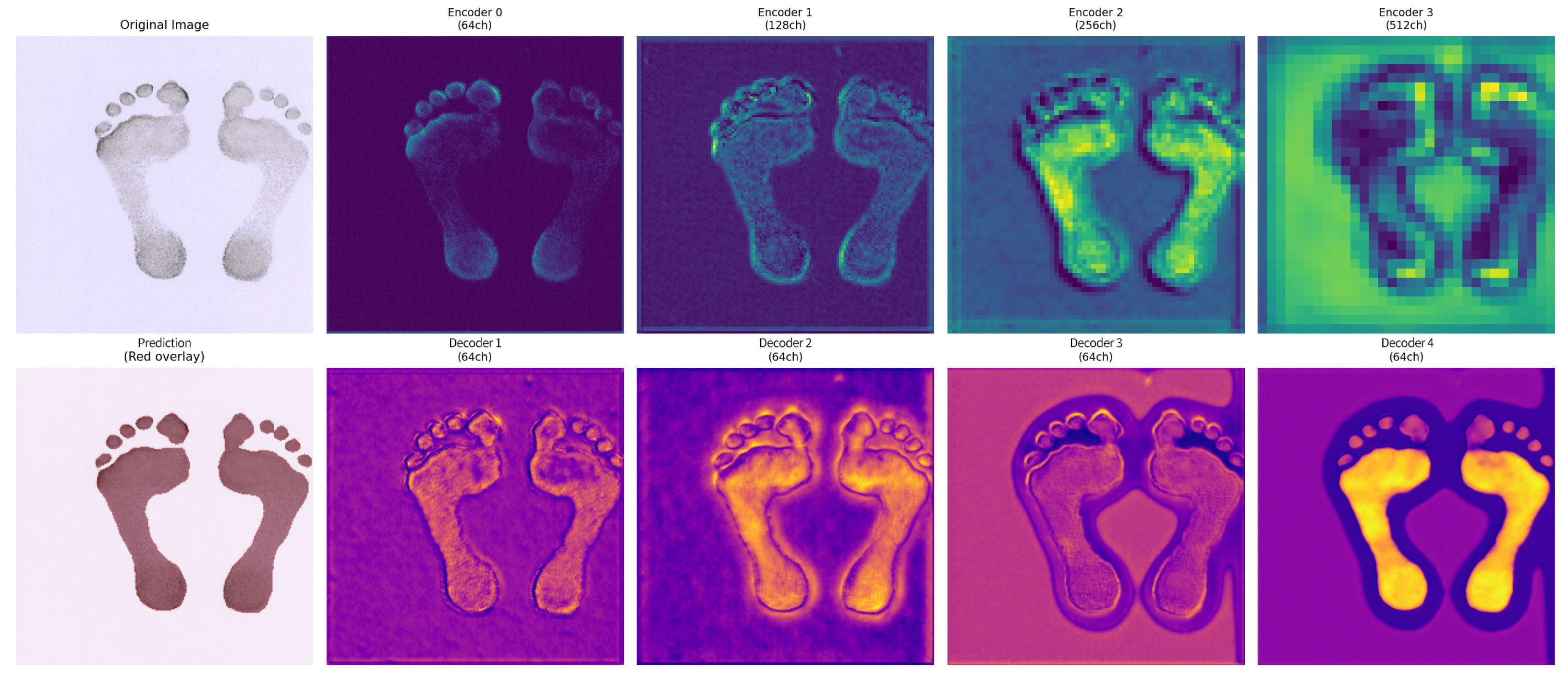
To investigate the feature patterns extracted at different levels by the model, we visualized the feature maps extracted by the encoder and decoder, as shown in Figure 5. Encoder feature analysis showed that the shallow encoders (Encoders 0–1) primarily capture edge details, texture, and local features of footprints, with their feature maps exhibiting distinct contour structures. As the network depth increases, the deep encoders (Encoders 2–3) progressively focus on higher-level semantic information such as the overall shape and regional structure of footprints, resulting in significantly more abstract feature representations. This demonstrates that the proposed model’s encoder effectively achieves feature extraction from local to global levels and from concrete to abstract representations. The decoder gradually integrates multi-scale features from the encoder through skip connections, restoring spatial resolution. Analysis of feature maps from Decoder 1 to Decoder 4 revealed that shallow decoders emphasize detail restoration, while deep decoders prioritize semantic information integration. The final prediction map localized the footprint and yielded contours that visually agreed with the corresponding footprint image.

4.2.8. Attention Visualization

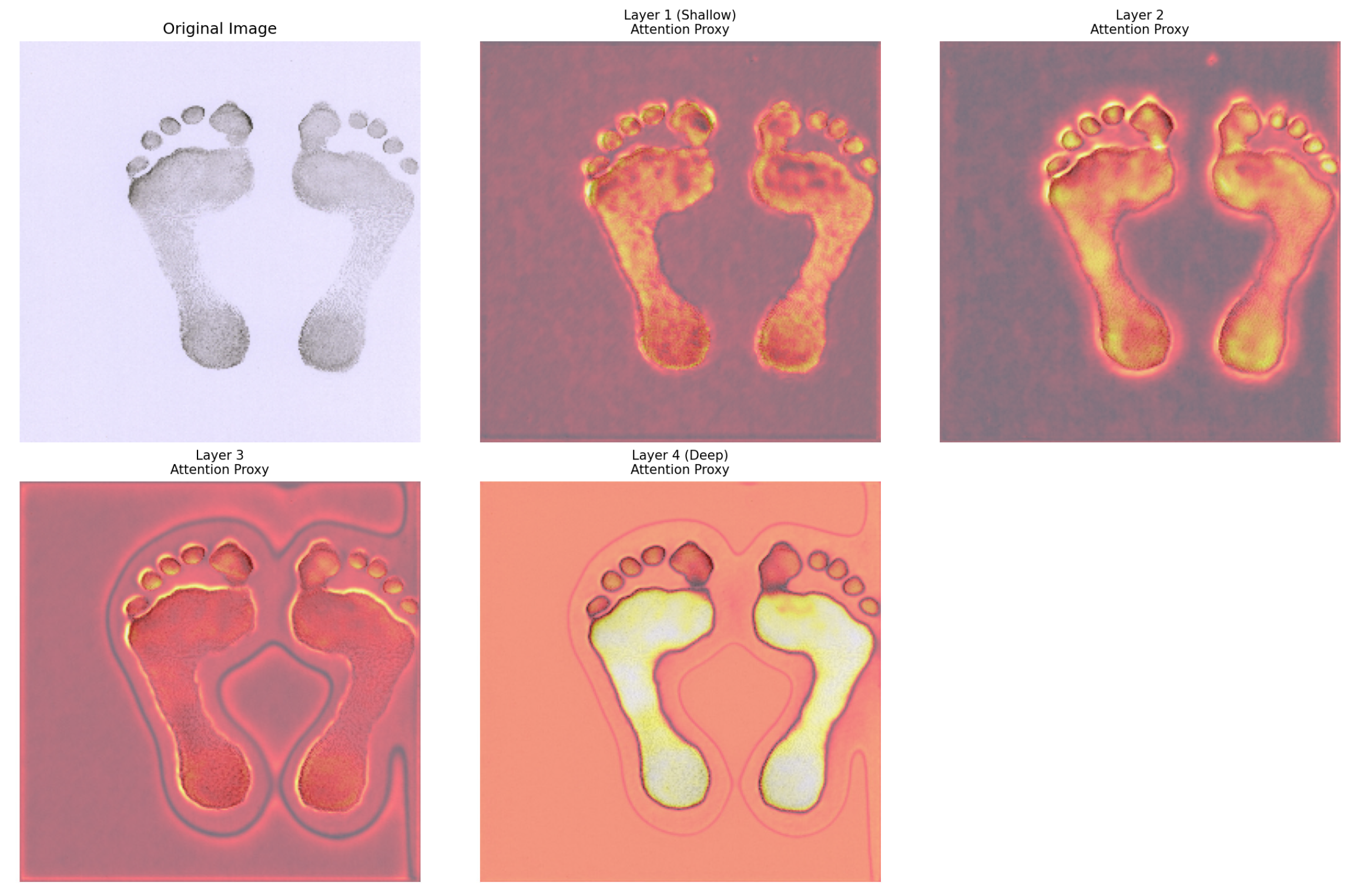
Channel-wise feature-map variance was visualized as an activation-intensity proxy rather than as a direct measurement of attention. The visualization suggests that the shallow decoder focuses on scattered local regions, whereas the deep decoder concentrates its attention on the core area of the footprint. This shift from dispersed to concentrated attention suggests a coarse-to-fine feature refinement process, effectively suppressing background interference, as illustrated in Figure 6.

4.2.9. Noise Robustness Analysis

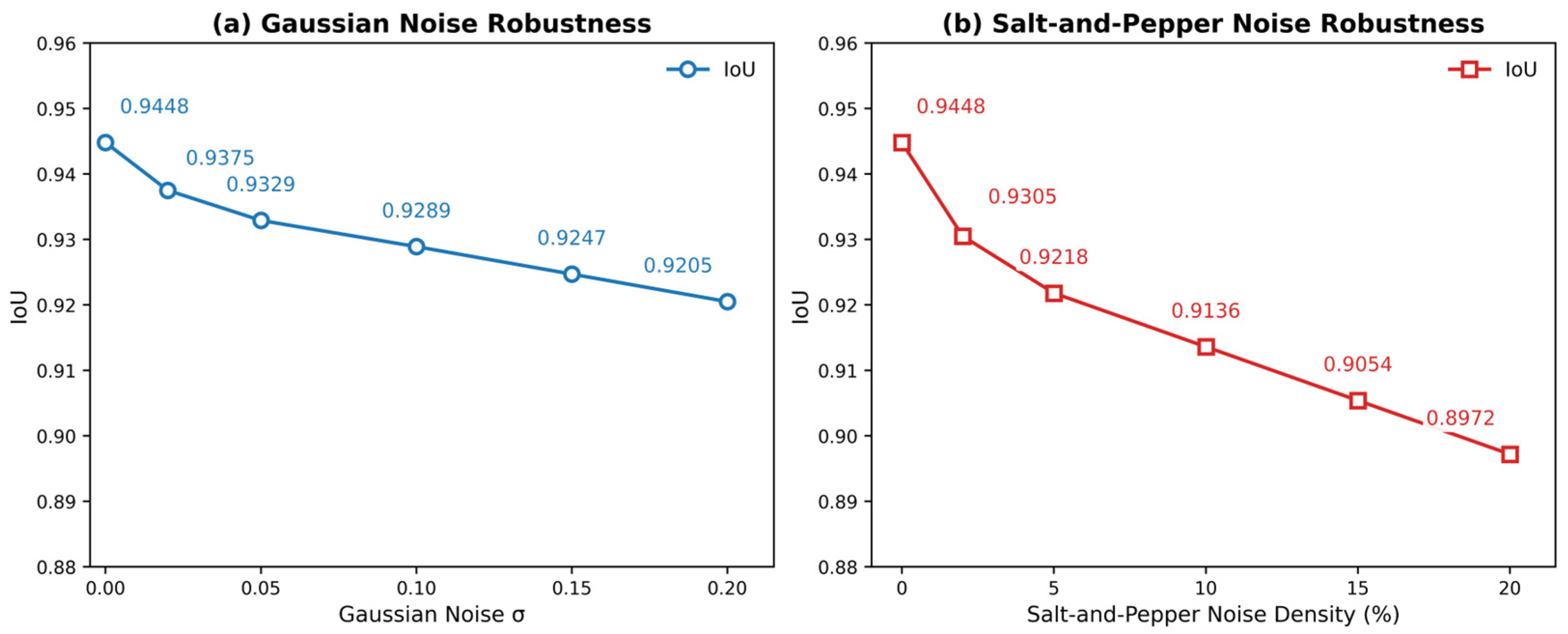
We evaluate the impact of two common noise types on model performance: Gaussian noise (σ = 0.02–0.20) and salt-and-pepper noise (density = 2–20%). Figure 7 presents the noise robustness test results.

Table 10. Noise robustness test results.

Gaussian Noise σ	IoU	Relative Performance (%)	Salt-and-Pepper Noise Density	IoU	Relative Performance (%)
0.00	0.9448	100.00	0%	0.9448	100.00
0.02	0.9375	99.23	2%	0.9305	98.49
0.05	0.9329	98.74	5%	0.9218	97.57
0.10	0.9289	98.32	10%	0.9136	96.70
0.15	0.9247	97.87	15%	0.9054	95.83
0.20	0.9205	97.43	20%	0.8972	94.96

presents the noise robustness test results. The model exhibits modest IoU reductions to low-intensity Gaussian noise (σ ≤ 0.05), with the IoU decreasing by only approximately 1.26%. When σ = 0.10, the IoU drops to 0.9289 (98.32% relative performance); when σ = 0.20, the IoU is 0.9205 (97.43% relative performance). This indicates that the model maintained relatively robust performance under the evaluated Gaussian-noise conditions. Figure 7 visualizes the performance trends across the evaluated noise levels.

Salt-and-pepper noise has a more pronounced impact on model performance. At a noise density of 2%, the IoU drops to 0.9305 (98.49% relative performance). When the noise density increases to 20%, the IoU decreases to 0.8972 (94.96% relative performance). This noise randomly sets numerous pixels to extreme values, disrupting the edge continuity of the footprint and compromising segmentation accuracy. It should be noted that the Gaussian and salt-and-pepper noise used in this experiment represent controlled synthetic perturbations. These conditions do not reproduce the full range of degradation encountered in operational forensic settings, such as partial or fragmented impressions, occlusion, contamination, and acquisition-device differences.

4.2.10. Height Prediction Results and Comparative Analysis

To explore whether segmentation quality influences subsequent morphology-based analysis, we conducted a footprint-based height-prediction experiment as an exploratory downstream evaluation. After binarization, 29-dimensional quantitative features were extracted from each footprint sample. These features comprised three categories: (1) 12 contour-based geometric features, including footprint length, width, aspect ratio, area, perimeter, convex hull area, convex hull perimeter, equivalent diameter, eccentricity, roundness, compactness, and the ratio of foot width to forefoot/heel width; (2) 7 Hu invariant moments, which characterize the global topological structure of the footprint and are invariant to translation, rotation, and scaling; and (3) 10 statistical and projection-based features, including the mean and variance of horizontal and vertical projections, peak position, skewness, kurtosis, center-of-gravity offset, and centroid coordinates.

Using these 29 features as input and height as the regression target, we constructed a random forest (RF) regressor. To evaluate the effectiveness of RF, Linear Regression [40], Ridge Regression, ElasticNet [41], and Gradient Boosting [42] were selected as comparison models. The evaluation metrics were mean absolute error (MAE), root mean square error (RMSE), and the proportion of samples with prediction error absolute values less than 1 cm, 3 cm, and 5 cm (denoted as <1 cm, <3 cm, and <5 cm, respectively, in percentage). The height prediction performance of each model on the test set is shown in

Table 11. Comparison of height prediction performance of different models.

Model	MAE (cm)	RMSE (cm)	<1 cm (%)	<3 cm (%)	<5 cm (%)
Random Forest	3.39	4.03	8.8	54.4	77.2
Gradient Boosting	3.51	4.25	17.5	50.9	71.9
ElasticNet	3.65	4.43	14.0	52.6	70.2
Ridge Regression	3.80	4.63	10.5	50.9	70.2
Linear Regression	4.02	4.99	12.3	52.6	66.7

.

As shown in Table 11, RF achieved the lowest MAE (3.39 cm) and RMSE (4.03 cm) among the evaluated regressors. However, its accuracy under the strict < 1 cm criterion was lower than that of Gradient Boosting. Therefore, the RF model showed better overall error control in this dataset, rather than uniformly superior performance under every error threshold.

To examine the influence of segmentation masks on this downstream task, we compared masks generated by the baseline GAN with those generated by the proposed improved GAN. Both settings used the same feature-extraction pipeline and identical RF model configuration. The results are presented in

Table 12. Comparison of height prediction performance of different segmentation models.

Model	MAE (cm)	RMSE (cm)	<1 cm (%)	<3 cm (%)	<5 cm (%)
Baseline GAN	3.52	4.18	9.2	52.8	75.1
Proposed GAN	3.39	4.03	8.8	54.4	77.2
Change (proposed − baseline)	−0.13	−0.15	−0.4	+1.6	+2.1

.

Compared with the baseline GAN, the proposed method reduced MAE from 3.52 cm to 3.39 cm and RMSE from 4.18 cm to 4.03 cm. The proportions of predictions within 3 cm and 5 cm increased by 1.6 and 2.1 percentage points, respectively. However, the proportion within 1 cm decreased slightly by 0.4 percentage points. Overall, these changes are small.

Accordingly, the downstream experiment should be interpreted as preliminary evidence that improved segmentation masks may provide slightly more consistent footprint morphology features for height prediction in the present dataset. The practical relevance of these findings requires further validation using larger and more diverse participant-independent datasets and additional acquisition conditions.

5. Conclusions

This paper presents a GAN-based method for footprint image segmentation evaluated on the self-collected aFoot_2025 dataset under controlled acquisition conditions. The main findings can be summarized as follows. A channel-prior convolutional attention module is incorporated into the GAN framework. The module employs multi-scale depthwise convolutions to extract spatial features. Channel prior weights are further used for adaptive feature calibration. Experimental results show that CPCA outperforms representative attention mechanisms, including SE, ECA, and CBAM on both IoU and Dice metrics, highlighting its advantages in preserving spatial details while leveraging channel priors. The BCE–Dice hybrid loss achieved the best overall performance in the loss comparison experiment. It outperforms both individual loss functions and alternative formulations, including Focal, Tversky, and Lovász Hinge losses. This combination effectively balances pixel-level accuracy and regional overlap, making it particularly suitable for footprint images with extreme foreground-to-background imbalance. The proposed GAN + CPCA architecture achieved an IoU of 0.9448 and a Dice coefficient of 0.9713 on the self-built aFoot_2025 dataset, highlighting the complementary benefits of adversarial learning and attention mechanisms. The model showed modest IoU reductions under the evaluated synthetic Gaussian-noise conditions; however, these experiments should not be interpreted as validation under realistic forensic degradation. Feature-map and attention visualizations provided qualitative illustrations of the hierarchical feature patterns learned by the model.

Limitations and Future Directions. Several limitations should be acknowledged. The present findings are based on a participant-independent split of a single, self-collected dataset acquired under controlled conditions. Although participant-level separation reduces the risk of identity-related information leakage between the training and test subsets, it remains an internal evaluation within the aFoot_2025 dataset and does not constitute external validation. Consequently, the generalizability of the proposed method to data acquired from different populations, devices, substrates, and acquisition environments remains unknown. Moreover, the evaluated Gaussian and salt-and-pepper noise conditions represent synthetic perturbations and do not reproduce the full range of degradation encountered in operational forensic settings. The downstream height-prediction experiment was also exploratory and should not be interpreted as establishing the operational reliability of footprint-based stature estimation. Therefore, the reported results should be interpreted as evidence of methodological performance within the present dataset rather than as evidence of operational forensic validity.

Future work will focus on collecting and validating more diverse, multi-source footprint datasets; evaluating performance under realistic degradation and occlusion conditions; and incorporating approaches that improve long-range contextual modeling and shape completion. These efforts may further improve the reliability and practical applicability of footprint segmentation in forensic settings.

References

1. Mukhra, R.; Krishan, K.; Kanchan, T. Bare footprint metric analysis methods for comparison and identification in forensic examinations: A review of literature. J. Forensic Leg. Med. 2018, 58, 101–112. [Google Scholar] [CrossRef] [PubMed]
2. Khalid, M.; Kameneva, T.; McCarthy, C. Forensic gender and stature identification from footprint images using machine learning. Forensic Sci. Int. 2026, 379, 112760. [Google Scholar] [CrossRef] [PubMed]
3. García-Mora, S.; Regife-Fernández, L.; Tovaruela-Carrión, N.; Manfredi Márquez, M.J.; Vázquez-Castro, M.; Álvarez-Cordero, J.; Correa-Rodríguez, R.; Castro-Méndez, A. Forensic stature estimation: A systematic review of the correlation between footprints and individual height. Forensic Sci. Med. Pathol. 2026, 22, 363–371. [Google Scholar] [CrossRef] [PubMed]
4. Wicaksono, R.B.; Aulia, S.; Hadiyoso, S.; Hidayat, B. Human height and weight classification based on footprint using Gabor wavelet and k-NN methods. J. Infotel 2022, 14, 101–107. [Google Scholar] [CrossRef]
5. Abuqadumah, M.M.A.; Ali, M.A.M.; Almisreb, A.A.; Duraković, B. Deep transfer learning for human identification based on footprint: A comparative study. Period. Eng. Nat. Sci. 2019, 7, 1300–1307. [Google Scholar] [CrossRef]
6. Jang, M.; Carriquiry, A.; Park, S. Enhancing forensic shoeprint analysis: Application of the Shoe-MS algorithm to challenging evidence. Sci. Justice 2025, 65, 101255. [Google Scholar] [CrossRef] [PubMed]
7. Shen, Y.; Jiang, X.; Zhao, Y.; Xie, W. Barefoot footprint detection algorithm based on YOLOv8-StarNet. Sensors 2025, 25, 4578. [Google Scholar] [CrossRef] [PubMed]
8. Zhou, X.; Zhang, Y.; Fan, X.; Wang, N.; Bao, W. MFID-200: A multimodal footprint dataset and spatial-temporal prompted transformer for identification. Pattern Recognit. 2026, 179, 113581. [Google Scholar] [CrossRef]
9. Goodfellow, I.; Pouget-Abadie, J.; Mirza, M.; Xu, B.; Warde-Farley, D.; Ozair, S.; Courville, A.; Bengio, Y. Generative adversarial nets. In Proceedings of the 27th International Conference on Neural Information Processing Systems (NIPS 2014), Montreal, QC, Canada, 8–13 December 2014; Volume 2, pp. 2672–2680. [Google Scholar]
10. Mao, X.; Li, Q.; Xie, H.; Lau, R.Y.K.; Wang, Z.; Smolley, S.P. Least squares generative adversarial networks. In Proceedings of the 2017 IEEE International Conference on Computer Vision (ICCV), Venice, Italy, 22–29 October 2017; pp. 2813–2821. [Google Scholar] [CrossRef]
11. Isola, P.; Zhu, J.-Y.; Zhou, T.; Efros, A.A. Image-to-image translation with conditional adversarial networks. In Proceedings of the 2017 IEEE Conference on Computer Vision and Pattern Recognition (CVPR), Honolulu, HI, USA, 21–26 July 2017; pp. 1125–1134. [Google Scholar] [CrossRef]
12. Luc, P.; Couprie, C.; Chintala, S.; Verbeek, J. Semantic segmentation using adversarial networks. In Proceedings of the NIPS Workshop on Adversarial Training, Barcelona, Spain, 9 December 2016; Available online: https://inria.hal.science/hal-01398049v1 (accessed on 1 July 2026).
13. Hoffman, J.; Wang, D.; Yu, F.; Darrell, T. FCNs in the wild: Pixel-level adversarial and constraint-based adaptation. arXiv 2016, arXiv:1612.02649. [Google Scholar]
14. Koziński, M.; Simon, L.; Jurie, F. An adversarial regularisation for semi-supervised training of structured output neural networks. In Proceedings of the 31st Conference on Neural Information Processing Systems (NIPS 2017), Long Beach, CA, USA, 4–9 December 2017; Available online: https://hal.science/hal-01713323 (accessed on 1 July 2026).
15. Souly, N.; Spampinato, C.; Shah, M. Semi supervised semantic segmentation using generative adversarial network. In Proceedings of the IEEE International Conference on Computer Vision (ICCV), Venice, Italy, 22–29 October 2017; pp. 5689–5697. [Google Scholar] [CrossRef]
16. Cheng, C.; Zhang, J.; Cheng, Y.; Jia, Z.; He, W. MS-STGAN: A dual-branch multi-scale spatio-temporal generative adversarial framework for incomplete EEG-based emotion recognition. Neural Netw. 2026, 204, 109203. [Google Scholar] [CrossRef] [PubMed]
17. Zang, L.; Lv, C.; Huang, M. Dual-branch collaborative GAN with multi-scale CBAM and anatomical topology coding for enhanced early HCC detection in CT. Sci. Rep. 2025, 15, 40082. [Google Scholar] [CrossRef] [PubMed]
18. Al-Khazraji, S.H.A.; Iqbal, H.; Rubio, J.B.; García, F.; Al-Kaff, A. Multi-scale dual discriminator generative adversarial network for gas leakage detection. Electronics 2025, 14, 3564. [Google Scholar] [CrossRef]
19. Nguyen, T.; Le, T.; Vu, H.; Phung, D. Dual discriminator generative adversarial nets. In Advances in Neural Information Processing Systems 30 (NIPS 2017); Guyon, I., von Luxburg, U., Bengio, S., Wallach, H., Fergus, R., Vishwanathan, S., Garnett, R., Eds.; Curran Associates, Inc.: Red Hook, NY, USA, 2017; pp. 2667–2677. [Google Scholar]
20. Wang, Q.; Xie, H.; Qu, H. Dual-channel fusion and dual-discriminator GAN for infrared and visible image fusion. Electron. Res. Arch. 2025, 33, 5471–5495. [Google Scholar] [CrossRef]
21. Zhao, L.; Long, J.; Zhong, T. A deep learning-based two-branch generative adversarial network for image de-raining. Sensors 2024, 24, 6724. [Google Scholar] [CrossRef] [PubMed]
22. Hu, J.; Shen, L.; Sun, G. Squeeze-and-excitation networks. In Proceedings of the IEEE/CVF Conference on Computer Vision and Pattern Recognition (CVPR), Salt Lake City, UT, USA, 18–22 June 2018; pp. 7132–7141. [Google Scholar] [CrossRef]
23. Wang, Q.; Wu, B.; Zhu, P.; Li, P.; Zuo, W.; Hu, Q. ECA-Net: Efficient channel attention for deep convolutional neural networks. In Proceedings of the IEEE/CVF Conference on Computer Vision and Pattern Recognition (CVPR), Seattle, WA, USA, 14–19 June 2020; pp. 11531–11539. [Google Scholar] [CrossRef]
24. Woo, S.; Park, J.; Lee, J.-Y.; Kweon, I.S. CBAM: Convolutional block attention module. In Proceedings of the European Conference on Computer Vision (ECCV), Munich, Germany, 8–14 September 2018; pp. 3–19. [Google Scholar] [CrossRef]
25. Huang, H.; Chen, Z.; Zou, Y.; Lu, M.; Chen, C.; Song, Y.; Zhang, H.; Yan, F. Channel prior convolutional attention for medical image segmentation. Comput. Biol. Med. 2024, 178, 108784. [Google Scholar] [CrossRef] [PubMed]
26. Wang, T.-C.; Liu, M.-Y.; Zhu, J.-Y.; Tao, A.; Kautz, J.; Catanzaro, B. High-resolution image synthesis and semantic manipulation with conditional GANs. In Proceedings of the IEEE/CVF Conference on Computer Vision and Pattern Recognition (CVPR), Salt Lake City, UT, USA, 18–22 June 2018; pp. 8798–8807. [Google Scholar] [CrossRef]
27. Zou, R.; Zhang, J.; Wu, Y. Skin lesion segmentation through generative adversarial networks with global and local semantic feature awareness. Electronics 2024, 13, 3853. [Google Scholar] [CrossRef]
28. Kumar, A.; Memon, I.; Sami, A.; Jo, Y.; Choi, J. Positional component-guided Hangul font image generation via deep semantic segmentation and adversarial style transfer. Electronics 2025, 14, 2699. [Google Scholar] [CrossRef]
29. Chen, J.; Zhu, S.; Luo, W. Instance segmentation of underwater images by using deep learning. Electronics 2024, 13, 274. [Google Scholar] [CrossRef]
30. Andreini, P.; Ciano, G.; Bonechi, S.; Graziani, C.; Lachi, V.; Mecocci, A.; Sodi, A.; Scarselli, F.; Bianchini, M. A two-stage GAN for high-resolution retinal image generation and segmentation. Electronics 2022, 11, 60. [Google Scholar] [CrossRef]
31. Ronneberger, O.; Fischer, P.; Brox, T. U-Net: Convolutional networks for biomedical image segmentation. In Medical Image Computing and Computer-Assisted Intervention—MICCAI 2015; Navab, N., Hornegger, J., Wells, W.M., Frangi, A.F., Eds.; Springer: Cham, Switzerland, 2015; pp. 234–241. [Google Scholar] [CrossRef]
32. Milletari, F.; Navab, N.; Ahmadi, S.-A. V-Net: Fully convolutional neural networks for volumetric medical image segmentation. In Proceedings of the 2016 Fourth International Conference on 3D Vision (3DV), Stanford, CA, USA, 25–28 October 2016; pp. 565–571. [Google Scholar] [CrossRef]
33. Taghanaki, S.A.; Zheng, Y.; Zhou, S.K.; Georgescu, B.; Sharma, P.; Xu, D.; Comaniciu, D.; Hamarneh, G. Combo loss: Handling input and output imbalance in multi-organ segmentation. Comput. Med. Imaging Graph. 2019, 75, 24–33. [Google Scholar] [CrossRef] [PubMed]
34. Lin, T.-Y.; Goyal, P.; Girshick, R.; He, K.; Dollár, P. Focal loss for dense object detection. In Proceedings of the 2017 IEEE International Conference on Computer Vision (ICCV), Venice, Italy, 22–29 October 2017; pp. 2980–2988. [Google Scholar] [CrossRef]
35. Abraham, N.; Khan, N.M. A novel focal Tversky loss function with improved attention U-Net for lesion segmentation. In Proceedings of the 2019 IEEE 16th International Symposium on Biomedical Imaging (ISBI), Venice, Italy, 8–11 April 2019; pp. 683–687. [Google Scholar] [CrossRef]
36. Yu, J.; Blaschko, M.B. The Lovász hinge: A novel convex surrogate for submodular losses. IEEE Trans. Pattern Anal. Mach. Intell. 2020, 42, 735–748. [Google Scholar] [CrossRef] [PubMed]
37. Gaál, G.; Maga, B.; Lukács, A. Attention U-Net based adversarial architectures for chest X-ray lung segmentation. arXiv 2020, arXiv:2003.10304. [Google Scholar] [CrossRef]
38. Yunianta, A. MSB-UNet: A multi-scale bifurcation U-Net architecture for precise segmentation of breast cancer in histopathology images. Computation 2026, 14, 62. [Google Scholar] [CrossRef]
39. Zhang, S.; Rao, Q.; Wang, L.; Tang, T.; Chen, C. KPV-UNet: KAN PP-VSSA UNet for remote image segmentation. Electronics 2025, 14, 2534. [Google Scholar] [CrossRef]
40. Zhang, K.; Cui, J.H.; Luo, Y.Z.; Fan, F.; Yang, M.; Li, X.H.; Zhang, W.; Deng, Z.H. Estimation of stature and sex from scapular measurements by three-dimensional volume-rendering technique. Leg. Med. 2016, 21, 58–63. [Google Scholar] [CrossRef] [PubMed]
41. Zou, H.; Hastie, T. Regularization and variable selection via the elastic net. J. R. Stat. Soc. Ser. B Stat. Methodol. 2005, 67, 301–320. [Google Scholar] [CrossRef]
42. Balzer, M.; Bergherr, E.; Hutter, S.; Hepp, T. Gradient boosting for Dirichlet regression models. AStA Adv. Stat. Anal. 2026, 110, 149–189. [Google Scholar] [CrossRef]
Figure 1. Overall framework of footprint image segmentation.
Electronics 15 03028 g001
Figure 2. Architecture of the CPCA module.
Electronics 15 03028 g002
Figure 3. Acquired footprint images.
Electronics 15 03028 g003
Figure 4. Annotation examples of footprint regions and keypoints. The numbers indicate the predefined IDs assigned to both footprint keypoints and annotated plantar regions.
Electronics 15 03028 g004
Figure 5. Visualization of footprint feature responses. The colors in the feature maps represent normalized activation intensity, where brighter colors indicate stronger feature responses and darker colors indicate weaker responses.
Electronics 15 03028 g005
Figure 6. Attention visualization of the proposed model at different network layers. Warmer and brighter colors indicate stronger attention responses, while darker colors indicate weaker responses.
Electronics 15 03028 g006
Figure 7. Noise robustness analysis under Gaussian and salt-and-pepper noise.
Electronics 15 03028 g007