A Short-Term Traffic Flow Prediction Model Based on IHO-CNN-BiLSTM-Attention

Abstract

Accurate short-term traffic flow prediction is crucial for managing macroscopic Intelligent Transportation Systems (ITS). To overcome limitations in capturing complex spatiotemporal dependencies and the severe challenges of hyperparameter tuning, this paper proposes IHO-CNN-BiLSTM-Attention, a novel hybrid deep learning framework. Specifically, a Convolutional Neural Network (CNN) extracts local spatial features, a Bidirectional Long Short-Term Memory (BiLSTM) network captures temporal dependencies, and an attention mechanism dynamically weights key timesteps. To maximize the architecture’s performance, an Improved Hippopotamus Optimization (IHO) algorithm is proposed for automatic hyperparameter optimization. The IHO algorithm effectively overcomes the premature convergence of traditional optimizers by integrating a Piecewise Linear Chaotic Map (PWLCM) for initialization, tangent-based non-linear adaptive weights, a Tangent Flight defense mechanism, and Lens Opposition-Based Learning (LOBL) for local optimum escape. Evaluated comprehensively across three distinct macroscopic traffic benchmark datasets (a multimodal intersection, METR-LA velocity, and PeMSD4 volume), the IHO algorithm first demonstrated statistically significant superiority on standard CEC benchmark functions. Subsequently, the proposed hybrid model achieved state-of-the-art traffic state classification performance, maintaining peak F1-Scores of 0.9798, 0.8436, and 0.9561 across the highly diverse datasets. It significantly outperformed both classical optimized baselines (e.g., PSO, GWO) and contemporary heavy deep learning architectures (e.g., ASTformer, DiffSTG) under severe class imbalance and varying topological conditions. This work offers a robust, scalable, and highly generalized spatiotemporal forecasting solution with strong theoretical guarantees for intelligent traffic control.

1. Introduction

Accurate short-term traffic flow prediction is the fundamental cornerstone of modern Intelligent Transportation Systems (ITS). In the context of rapid urbanization, anticipating traffic conditions in advance is crucial for dynamic signal control, congestion mitigation, and emergency vehicle routing. However, urban traffic flow is highly volatile, exhibiting complex non-linear diurnal patterns and high-frequency noise caused by multi-modal commuting behaviors (e.g., the mixed flow of cars, buses, and trucks) [1]. Consequently, developing a robust predictive model capable of capturing these intricate spatiotemporal dynamics remains a formidable challenge [2].

Historically, traffic flow prediction has evolved from classical statistical models to sophisticated deep learning architectures [3]. While traditional methods like ARIMA struggle with non-stationary data [4], single deep learning models such as Convolutional Neural Networks (CNN) or Long Short-Term Memory (LSTM) networks excel in capturing either spatial or temporal features independently [5]. Recently, hybrid spatiotemporal models combined with attention mechanisms and multivariate clustering approaches have demonstrated state-of-the-art performance by dynamically weighting critical historical moments and grouping correlated trends.

Despite these architectural advancements, a critical methodological gap remains: the prediction accuracy of these highly complex, multivariate networks is strictly bounded by their hyperparameter configurations. The manual tuning of parameters (e.g., learning rates, network depth, and attention heads) in continuous high-dimensional spaces is computationally prohibitive. While traditional meta-heuristic algorithms like Particle Swarm Optimization (PSO) and Grey Wolf Optimizer (GWO) have been introduced to automate this process, they frequently suffer from premature convergence and poor exploration–exploitation trade-offs when navigating the rugged loss landscapes of deep neural networks, ultimately leading to suboptimal traffic forecasting.

To overcome the limitations of spatiotemporal feature extraction and the severe bottleneck of hyperparameter tuning, this paper proposes IHO-CNN-BiLSTM-Attention, a novel hybrid deep learning framework [6]. Specifically, a CNN is utilized to extract local spatial grid features, a Bidirectional LSTM (BiLSTM) network captures forward and backward temporal dependencies, and an attention mechanism dynamically highlights critical time steps [7]. To maximize the performance of this complex architecture, an Improved Hippopotamus Optimization (IHO) algorithm is proposed. By integrating a Piecewise Linear Chaotic Map (PWLCM) for initialization, tangent-based non-linear adaptive weights, a Tangent Flight defense mechanism, and Lens Opposition-Based Learning (LOBL), the IHO mathematically guarantees a superior balance between global exploration and local exploitation to find the optimal network configuration [8].

The main contributions of this paper are summarized as follows:

• A Novel Hybrid Spatiotemporal Architecture: We frame short-term traffic prediction as a discrete classification task to align with macroscopic ITS decision-making. A CNN-BiLSTM-Attention framework is constructed to comprehensively capture non-linear spatiotemporal traffic dynamics and filter high-frequency noise.
• An Improved Meta-Heuristic Optimizer (IHO): To address the hyperparameter tuning bottleneck, the IHO algorithm is proposed. By integrating PWLCM initialization, Tangent Flight, tangent-based non-linear weights, and LOBL mechanisms, IHO mathematically guarantees a superior balance between global exploration and local exploitation compared to existing algorithms.
• Comprehensive and Robust Experimental Validation: Extensive experiments on complex CEC benchmark functions rigorously prove the statistical superiority of the IHO algorithm. Furthermore, the overall framework was evaluated on three distinct, large-scale macroscopic traffic datasets (encompassing highly imbalanced velocity data and perfectly balanced volume data). The results confirm that our dynamically optimized architecture achieves state-of-the-art generalization performance, decisively outperforming unoptimized parameter-heavy SOTA models (such as Spatial-Temporal Transformers and Diffusion-based networks).

The paper is structured in the following way:

Section 2 provides a comprehensive review of recent advances in traffic flow prediction and Intelligent Transportation Systems (ITS), highlighting key contributions from leading international journals. Section 3 introduces the Hippopotamus Optimization (HO) algorithm and its enhanced version (IHO) with Latin Hypercube Sampling and Levy Flight strategies, followed by a detailed exposition of the proposed IHO-CNN-BiLSTM-Attention model, including its architecture, algorithmic principles, and theoretical foundations. Section 4 outlines the experimental framework, covering dataset selection, comparative model configurations, evaluation metrics, and analysis of results across original augmented datasets. Section 5 concludes the study by summarizing the model’s contributions, discussing limitations, and proposing future research directions such as real-time adaptation and multimodal data fusion.

2. Related Work

To properly contextualize the proposed IHO-CNN-BiLSTM-Attention framework, this section critically reviews existing literature by categorizing it into four distinct methodological families. We analyze the progressive advancements and identify the residual limitations within each family that motivate our research.

2.1. Classical Statistical and Machine Learning Models

Early traffic flow prediction heavily relied on classical statistical time-series analysis and traditional machine learning methods. For instance, Auto-Regressive Integrated Moving Average (ARIMA) models have been widely used to fit traffic trajectories based on historical sliding windows. Similarly, machine learning approaches like Support Vector Regression (SVR) and Random Forests have been utilized to map historical numerical features to future traffic volumes [9,10]. While these models establish foundational forecasting paradigms and are computationally efficient, their fundamental limitation is the assumption of stationarity and shallow feature mapping. Consequently, they inherently struggle to capture the complex, highly dynamic, and non-linear spatiotemporal fluctuations characteristic of real-world urban traffic networks, leading to rapid performance degradation under sudden congestion scenarios [11].

2.2. Single and Hybrid Deep Learning Architectures

To address the non-linear nature of traffic data, deep learning architectures have become the mainstream approach. Recurrent Neural Networks, particularly LSTM and Gated Recurrent Units (GRU), are heavily relied upon to memorize sequential temporal dependencies and overcome the vanishing gradient problem [12]. Simultaneously, Convolutional Neural Networks (CNN) excel at extracting localized spatial grid features. Recognizing that urban traffic prediction requires modeling both domains, researchers introduced hybrid spatiotemporal models. For example, recent studies have demonstrated that CNN-LSTM or CNN-BiLSTM frameworks can significantly enhance predictive accuracy by simultaneously modeling spatial dependencies and temporal dynamics [13]. While these hybrid models successfully capture multi-dimensional features, they inherently possess a structural drawback: they typically treat all historical time steps equally. This uniform treatment fails to distinguish between critical inflection points (e.g., a sudden traffic accident) and routine daily noise, thereby limiting the model’s responsiveness.

2.3. Attention Mechanisms and Multivariate Clustering Approaches

To overcome the uniform-weighting limitation of hybrid RNNs, the Attention mechanism was introduced to dynamically assign varying weights to different time steps, emphasizing critical historical moments for future state prediction [14]. Furthermore, urban traffic datasets are inherently multi-modal and multivariate (e.g., correlated flows of cars, bikes, and buses). Recognizing this, recent state-of-the-art research has shifted towards multivariate correlation and clustering-based prediction approaches. Notably, Pellicani et al. (2025) proposed a framework for the simultaneous prediction of anomalies from groups of correlated multivariate time series [15], demonstrating that clustering-based approaches for correlated trends can significantly enhance prediction robustness by grouping similar temporal patterns before forecasting. Such multivariate pattern recognition aligns perfectly with the multi-modal nature of our traffic dataset. However, the integration of attention networks and multivariate correlation processing drastically increases the architectural complexity and parameter space [16,17].

2.4. Meta-Heuristic Hyperparameter Optimization

The extreme sensitivity of complex hybrid models (such as CNN-BiLSTM-Attention) to their hyperparameter configurations presents a critical engineering bottleneck [18]. Manual tuning or grid search is computationally prohibitive in continuous high-dimensional spaces. Consequently, meta-heuristic algorithms have been actively employed to automate hyperparameter selection in traffic prediction. Studies have utilized Particle Swarm Optimization (PSO) and Grey Wolf Optimizer (GWO) to optimize the window sizes and learning rates of deep LSTM networks, achieving better accuracy than empirical tuning [19]. Despite their utility, traditional optimizers suffer from severe limitations. When navigating the rugged and deceptive loss landscapes of deep neural networks, algorithms like PSO are prone to premature convergence, failing to effectively balance global exploration with local exploitation.

The literature review reveals a clear trajectory: while hybrid models with attention mechanisms handle complex multivariate traffic data effectively, their performance is fundamentally bottlenecked by suboptimal hyperparameter configurations and the premature convergence of traditional optimizers. This critical gap motivates the development of our Improved Hippopotamus Optimization (IHO) algorithm, designed to provide a mathematically guaranteed optimal parameter search for deep learning traffic forecasting [20].

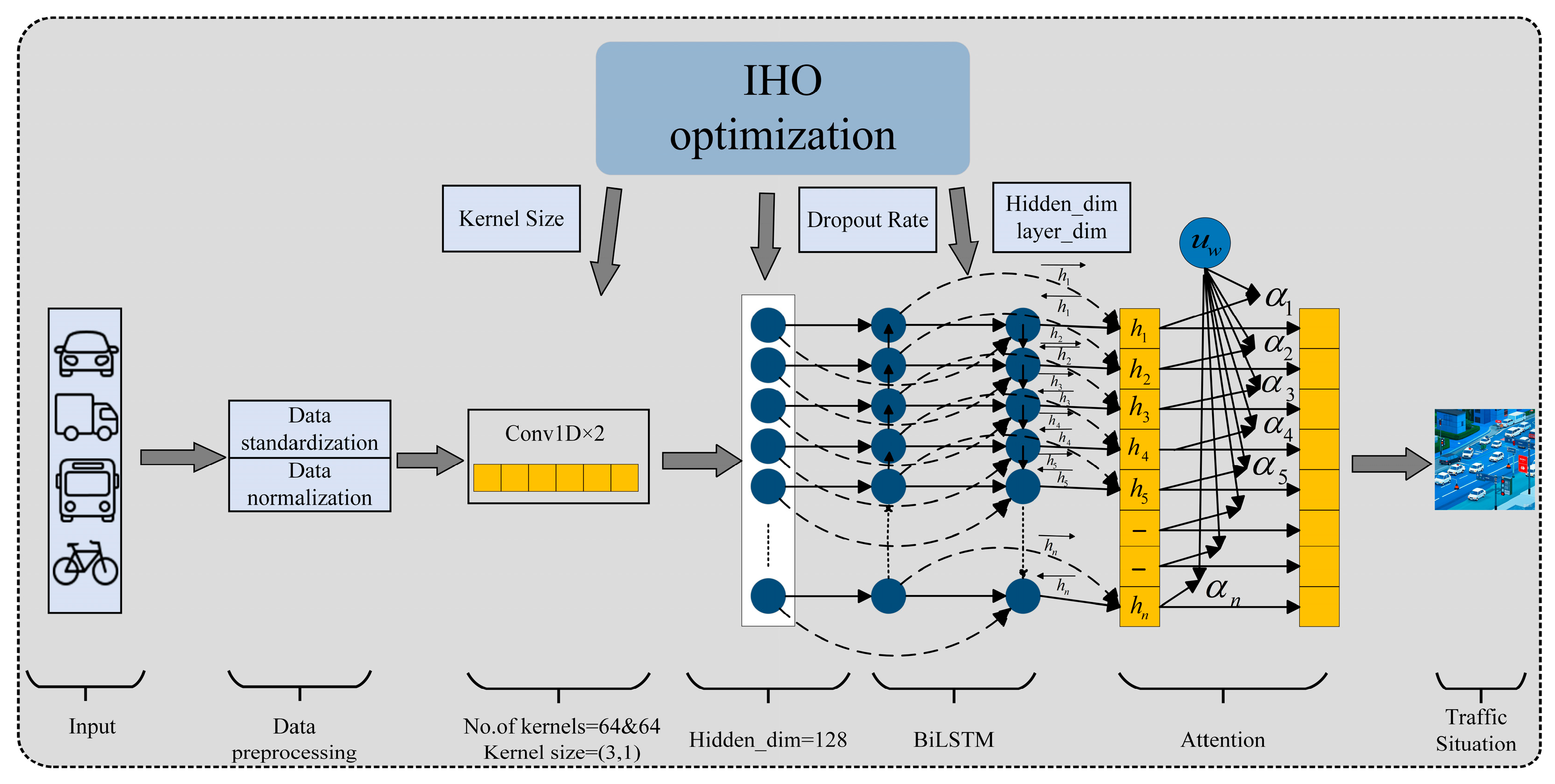
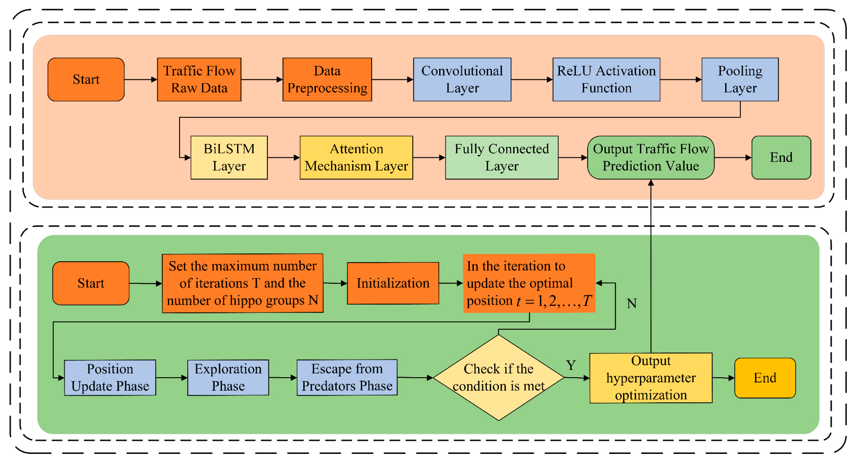
In summary, there have been notable strides in traffic flow prediction research in recent years, particularly in the application of deep learning and spatiotemporal techniques. However, existing CNN-BiLSTM models and Attention mechanisms still face many challenges, especially in improving the ability to capture key spatiotemporal features and optimizing hyperparameters. Therefore, this paper proposes a hybrid model based on CNN, BiLSTM, and Attention mechanisms (CNN-BiLSTM-Attention), using an improved Hippopotamus Optimization Algorithm (IHO) to optimize hyperparameters, aiming to enhance the accuracy and robustness of traffic flow prediction. The flowchart of the specific model architecture and hyperparameter optimization is shown in Figure 1.

3. Materials and Methods

This section details the various modules and the overall construction process of the IHO-CNN-BiLSTM-Attention model, which includes the enhanced Hippopotamus Optimization Algorithm (IHO), Convolutional Neural Network (CNN), Bidirectional Long Short-Term Memory Network (BiLSTM), and Attention Mechanism, and describes the overall approach to model development.

3.1. Introduction and Improvement Strategies of the Hippopotamus Optimization Algorithm

3.1.1. Hippopotamus Optimization Algorithm

The Hippopotamus Optimization Algorithm (HO) is inspired by the behavior of hippos in their natural environment, simulating their position updates in water, defense strategies, and predator-evading behaviors. The HO algorithm seeks to improve both global and local search efficiency to tackle complex optimization problems by simulating these behaviors. The algorithm was first published by Mohammad Hussein Amiri et al. in Scientific Reports in February 2024 [8].

• Position Update Phase (Exploration Phase): This phase simulates the behavior of hippos updating their position in water, primarily used for global search. The mathematical expression is as follows:

$$X_i^{new}=X_i^{current}+y_1\cdot (D_{hippo}-I_1\cdot X_i^{current})$$

(1)

In Equation (1), $X_i^{new}$ is the new position of the $i$-th hippo, $X_i^{current}$ is the current position, $D_{hippo}$ is the current best (dominant) hippo position, $I_1$ is an integer, and $y_1$ is a random number.

2.

Defense Phase (Exploration Phase): This phase simulates the defensive behavior of hippos when facing threats. If a predator approaches, the hippo adjusts its position to avoid being preyed upon. The related position update formula is as follows:

$${\chi }_i^{HippoR}=RL\oplus Predato{r}_j+f\cdot (c-d\times \cos (2\pi g))\cdot {\displaystyle \frac{1}{D}}$$

(2)

In Equation (2), $Predato{r}_j$ represents the position of the predator, ${\chi }_i^{HippoR}$ represents the hippo’s defensive position, $D$ represents the distance between the $i$-th hippo and the predator, and $RL$ denotes a random disturbance vector to defend against threats and maintain exploration balance.

3.

Predator Evasion Phase (Exploitation Phase): When a hippo faces multiple predators or cannot defend itself, it escapes to the nearest safe location. This phase is primarily used for local search optimization. The position update formula is:

$${\chi }_i^{HippoE}={\chi }_i+r_{10}\cdot (l{b}_{local}+s_1\cdot (u{b}_{local}-l{b}_{local}))$$

(3)

In Equation (3), where $r_{10}$ and $s_1$ are random numbers used to generate a new position near the hippo’s current position, optimizing local exploitation. Where $l{b}_{local}$ and $u{b}_{local}$ denote the lower and upper bounds of the local search space, respectively.

3.1.2. Specific Improvements of the Hippopotamus Optimization Algorithm

The original Hippopotamus Optimization (HO) algorithm has limitations in handling high-dimensional complex data, including uneven initial population distribution, rigid linear parameter control, and the high computational overhead of Lévy flight. To overcome these constraints and tailor the algorithm for the hyperparameter optimization of deep learning models, this study proposes an Improved Hippopotamus Optimization (IHO) algorithm by integrating four advanced strategies:

1.

Piecewise Linear Chaotic Map (PWLCM) Initialization [21]: Instead of traditional pseudo-random initialization, which often results in local clustering and search blind spots, IHO utilizes PWLCM to construct a highly ergodic and uniform initial population topology. This guarantees a broader exploration of the initial hyperparameter search space. The initialization is mathematically defined as:

$$x_{i,j}={\mathrm{lb}}_j+z_{i,j}\times \left({\mathrm{ub}}_j-{\mathrm{lb}}_j\right)$$

(4)

In Equation (4), $X_{i,j}$ denotes the initial position of the $i$-th hippo individual in the $i$-th dimension; $l{b}_j$ and $u{b}_j$ represent the lower and upper bounds of the $j$-th decision variable, respectively; $z_{i,j}$ is the chaotic sequence generated by the PWLCM in the range of $(0,1)$.

2.

Tangent Non-linear Adaptive Inertia Weight [22]: To dynamically balance global exploration in the early stages and local exploitation in the later stages, a non-linear adaptive inertia weight ($\omega$) based on the tangent function is introduced. Unlike traditional linear decay, the tangent-based weight maintains a slow decline initially to prevent premature convergence and drops sharply later to accelerate exact convergence.

$$\omega \left(t\right)={\omega }_{\min }+\left({\omega }_{\max }-{\omega }_{\min }\right)\cdot \tan \left[{\displaystyle \frac{\pi }{4}}\cdot \left(1-{\left({\displaystyle \frac{t}{T_{\max }}}\right)}^k\right)\right]$$

(5)

In Equation (5), $\omega (t)$ is the adaptive inertia weight at the current iteration $t$; $T_{max}$ denotes the maximum number of iterations; ${\omega }_{max}$ and ${\omega }_{\min }$ are the predefined maximum and minimum weight values, respectively; and $k$ is the non-linear adjustment exponent which controls the curvature of the weight decay.

3.

Tangent Flight Strategy for Evasion [23]: The original HO relies on Lévy flight during the predator evasion phase. However, the heavy-tailed nature of Lévy flight often causes unbounded jumps, boundary violations, and high computational costs. To address this, IHO introduces the Tangent Flight strategy. By exploiting the mathematical singularity of the tangent function, it provides a smoother, more controllable transition between large exploratory jumps and small exploitative steps, significantly reducing computational overhead while ensuring global reachability. The step size factor is updated as:

$$S_{\tan }=\mathrm{step}\_\mathrm{size}\times \tan \left(\theta \right)$$

(6)

$$x_{i,j}^{\mathrm{new}}\left(t\right)=x_{i,j}\left(t\right)+A\left(t\right)\cdot \tan \left(\theta \right)\cdot \left|x_{\mathrm{best},j}\left(t\right)-x_{i,j}\left(t\right)\right|$$

(7)

In Equation (7), $f_t$ represents the tangent flight step size factor; $\theta$ is a random angle uniformly distributed in the interval $(-\pi /2,\pi /2)$; $A(t)$ denotes the adaptive amplitude factor used to restrict the step size as iterations progress; and $X_i^{new}$ and $X_i^{current}$ represent the updated and current positions of the hippo, respectively.

4.

Lens Opposition-Based Learning (LOBL) [24]: To prevent the algorithm from stagnating at local optima during the late iterations, a Lens Opposition-Based Learning mechanism is applied as a post-processing step. Modeled after the optical imaging principle of a convex lens, LOBL generates an opposite conjugate solution within the dynamically shrinking boundaries of the current population. This mechanism forces the algorithm to explore the symmetrical regions of the current best solution, thus providing a deterministic escape route from local traps. The LOBL conjugate solution is formulated as:

$$X_t^{i+1}=X_t^i+ϵ\cdot \mathcal{N}(0,0.01)$$

(8)

In Equation (8), $ϵ$ is a small perturbation coefficient, and $\mathcal{N}(0,0.01)$ represents a random perturbation following a normal distribution. In the LOBL formula, $X_{best}^{*}$ denotes the generated opposition (reflected) solution; $X_{best}$ is the current global optimal solution acting as the ‘object’; $a_j$ and $b_j$ are the dynamic lower and upper boundaries of the $j$-th dimension in the current population; $k$ represents the scaling factor or the ‘magnification’ of the lens, which balances the distance of the reflected solution from the search center.

3.2. Execution Framework and Pseudocode of the IHO Algorithm

The execution of the proposed IHO algorithm follows a structured optimization process to effectively balance global exploration and local exploitation. Initially, the hippo population is uniformly generated using the Piecewise Linear Chaotic Map (PWLCM). During the iterative process, the algorithm dynamically adjusts its search steps via tangent-based non-linear weights and executes the Tangent Flight strategy to evade local optima. Finally, a Lens Opposition-Based Learning (LOBL) mechanism is applied as a post-processing step to guarantee deterministic escapes from stagnation. The systematic workflow of the IHO algorithm detailed implementation is summarized in Algorithm 1.

Algorithm 1. IHO

Input: Population size $N$$, \mathrm{Maximum} \mathrm{iterations} T_{max}$, Dimension $D$$, \mathrm{Lower} \mathrm{and} \mathrm{Upper} \mathrm{bounds} lb,ub$

Output:$\mathrm{Global} \mathrm{optimal} \mathrm{position} X_{best}$ and its fitness value

1. $\mathrm{Initialize} \mathrm{the} \mathrm{hippo} \mathrm{population} X=\{X_1,X_2,\dots ,X_N\}$ using Piecewise Linear Chaotic Map (PWLCM) 2. $\mathrm{Set} \mathrm{iteration} \mathrm{counter} t=1$ 3. While $t\le T_{max}$ do 4. Calculate the fitness value for each individual in the population 5. $\mathrm{Identify} \mathrm{the} \mathrm{dominant} \mathrm{hippo} (\mathrm{current} \mathrm{best} \mathrm{solution}) \mathrm{as} X_{best}$ 6. Update the non-linear adaptive inertia weight $\omega (t)$ and amplitude factor $A(t)$ using Tangent functions 7. For each individual $i$ from 1 to $N$ do 8. // Phase 1: Position Update (Exploration) 9. $\mathrm{Update} \mathrm{the} \mathrm{individual}’\mathrm{s} \mathrm{position} \mathrm{towards} X_{best}$$\mathrm{or} \mathrm{population} \mathrm{mean}, \mathrm{dynamically} \mathrm{adjusted} \mathrm{by} \omega (t)$ 10. // Phase 2: Predator Defense (Extremum Escape) 11. Execute the Tangent Flight strategy to evade virtual predators and generate a new position 12. // Phase 3: Predator Evasion (Exploitation) 13. Perform local fine-tuning near the current position to simulate escaping to safe waters 14. End For 15. // Phase 4: Lens Opposition-Based Learning (LOBL) Post-processing 16. Calculate the dynamic boundaries of the current population 17. $\mathrm{Generate} \mathrm{an} \mathrm{opposition} \mathrm{conjugate} \mathrm{solution} X_{best}^{*}$$\mathrm{based} \mathrm{on} \mathrm{the} \mathrm{current} X_{best}$ using LOBL 18. If $f(X_{best}^{*})<f(X_{best})$ then 19. $X_{best}=X_{best}^{*}$ (Greedy selection) 20. End If 21. $t=t+1$ 22. End While 23. Return$\mathrm{the} \mathrm{global} \mathrm{optimal} \mathrm{position} X_{best}$

3.3. Construction of the IHO-CNN-BiLSTM-Attention Model

3.3.1. Convolutional Neural Network (CNN) Feature Extraction

The first module of the model is the Convolutional Neural Network (CNN) [25], which is responsible for extracting local spatial features from the input data. The input traffic flow data undergoes two layers of one-dimensional convolution operations, with the calculation formula for each convolution layer as follows:

$$F_{i,j,k}={\displaystyle \sum _{m,n}{X}_{i+m,j+n} · W_{m,n,k} +} b_k$$

(9)

In Equation (9), $F_{i,j,k}$ is the convolution output, $W$ is the convolution kernel weight, $b_k$ is the bias term, $i,j$ are the data positions, and $k$ is the number of channels. The convolutional layer uses the ReLU activation function to handle nonlinear features and further reduces dimensionality through max pooling. The pooling formula is as follows:

$$P_{i,j}=max\left(X_{i+m,j+n}\right), m,n\in \mathrm{kernel} \mathrm{size}$$

(10)

3.3.2. Bidirectional Long Short-Term Memory Network

The Bidirectional Long Short-Term Memory Network (BiLSTM) receives the pooled features to capture temporal dependencies in the input data [26]. It consists of a forward and a backward LSTM layer, with the respective calculation formulas and the final output formula given as follows:

$${\overrightarrow{h}}_t=f(W_{\overrightarrow{h}}\cdot x_t+U_{\overrightarrow{h}}\cdot {\overrightarrow{h}}_{t-1}+b_{\overrightarrow{h}})$$

(11)

$${\overleftarrow{h}}_t=f(W_{\overleftarrow{h}}\cdot x_t+U_{\overleftarrow{h}}\cdot {\overleftarrow{h}}_{t+1}+b_{\overleftarrow{h}})$$

(12)

$$h_t=[\overrightarrow{h_t},\overleftarrow{h_t}]$$

(13)

where $W_{\overrightarrow{h}},U_{\overrightarrow{h}},b_{\overrightarrow{h}}$ and $W_{\overleftarrow{h}},U_{\overleftarrow{h}},b_{\overleftarrow{h}}$ represent the independent weight matrices and bias vectors for the forward and backward LSTM layers, respectively.

3.3.3. Attention Mechanism

The time-step hidden states output by the BiLSTM are fed into the attention mechanism to highlight the influence of key time steps [17]. The attention weights are calculated using the following formula:

$$e_t=\tanh (W_a{h}_t+b_a)$$

(14)

$${\alpha }_t={\displaystyle \frac{\exp (e_t)}{{\displaystyle \sum _k}\exp (e_k)}}$$

(15)

The final aggregated output is:

$$v=\sum _t{\alpha }_t{h}_t$$

(16)

where ${\alpha }_t$ is the weight at time step $t$, and $v$ is the weighted feature vector.

3.3.4. Fully Connected Layer and Output

The attention mechanism’s output is then fed into the fully connected layer for predicting the traffic flow classification results [27]. The classification loss function adopts cross-entropy:

$$L=-{\displaystyle \sum _{i=1}^C}{y}_i\log ({\widehat{y}}_i)$$

(17)

where $y_i$ and ${\widehat{y}}_i$ represent the true class and predicted class probabilities, respectively, and $C$ is the number of classes.

3.4. Model Framework and Pseudocode

By integrating Convolutional Neural Networks (CNN), Bidirectional Long Short-Term Memory Networks (BiLSTM), and an Attention Mechanism, the model utilizes the Improved Hippopotamus Optimization Algorithm (IHO) to fine-tune its hyperparameters.

The model integration begins with the Convolutional Neural Network (CNN), which extracts local features from the data through convolution and pooling layers. The output of the convolution layer is passed through the ReLU activation function and pooled to reduce dimensionality. The resulting features are then fed into the Bidirectional Long Short-Term.

The Memory Network (BiLSTM) processes the sequential data via forward and backward LSTM layers to capture bidirectional dependencies. The output of the BiLSTM is directed through an Attention Mechanism, allowing the model to focus on key time steps and features, thereby extracting more relevant information. Finally, the features enhanced by the attention mechanism are input into a fully connected layer for classification [6,13].

For hyperparameter optimization, the improved Hippo Optimization Algorithm (IHO) is used to optimize the model’s hyperparameters, such as the hidden layer dimensions, number of layers, learning rate, and dropout rate of LSTM. The IHO algorithm simulates the foraging and social behaviors of hippos, finding the optimal parameter combinations through global search and local development [28,29,30]. The specific structure is shown in Figure 2.

4. Results Data Selection and Experiments

4.1. Dataset Description

4.1.1. Multimodal Intersectional Dataset

The dataset used in this study is sourced from the publicly available “Traffic Prediction Dataset” on Kaggle (https://www.kaggle.com/datasets/hasibullahaman/traffic-prediction-dataset) (accessed on 15 January 2026) [31]. It is a comprehensive multi-modal traffic dataset derived from IoT sensor records at a typical urban arterial intersection. As illustrated in Figure 3a, the dataset covers a continuous time span of exactly 31 days (one month), with a sampling granularity of 15 min. This fine-grained sampling results in a total of 2976 continuous temporal observations. Each observation captures the aggregated multi-modal traffic volume, including the counts of cars, bikes, buses, and trucks, reflecting the complex, non-linear diurnal patterns of urban commuting. As shown in Figure 3b, the dataset categorizes the overall traffic situation into four distinct congestion levels (Heavy, High, Normal, Low) based on the total vehicle counts.

To rigorously evaluate the spatiotemporal forecasting capability of the proposed model and to strictly prevent any potential “data leakage”, we entirely prohibited random shuffling during the data splitting process. Instead, a strict chronological sequential split was employed:

• Training Set (70%): The first 21 days (approximately 2083 time steps) were used exclusively for model training and structural learning.
• Validation Set (10%): The subsequent 3 days (approximately 298 time steps) were utilized for hyperparameter tuning and early stopping condition monitoring.
• Test Set (20%): The final 7 days (approximately 595 time steps) were strictly reserved as unseen future data to evaluate the final model’s generalization capability. This strict preservation of temporal ordering guarantees a realistic and scientifically robust evaluation of the time-series model.

4.1.2. METR-LA Dataset

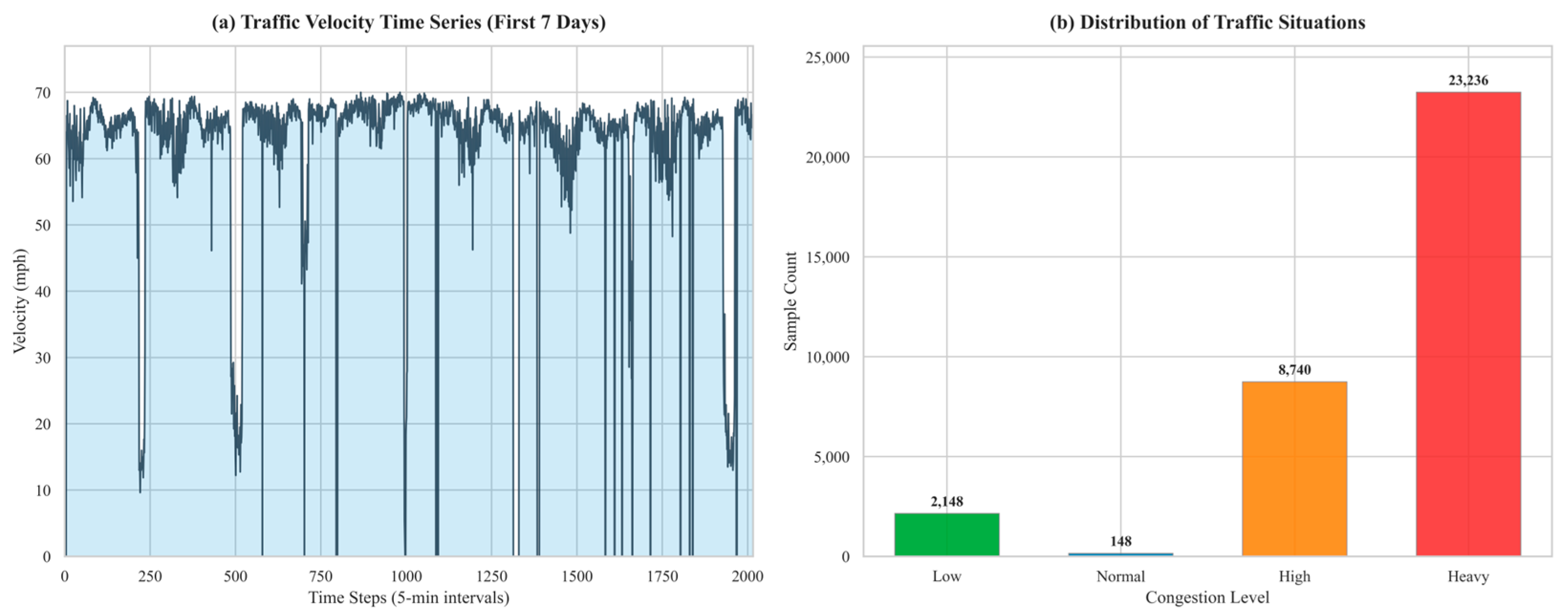
To comprehensively evaluate the generalization capability and robustness of the proposed IHO-CNN-BiLSTM-Attention framework, the international benchmark METR-LA dataset is introduced. Sourced from the highway network of Los Angeles, California, this dataset contains continuous traffic velocity records compiled from $N=207$ inductive loop sensors. The temporal span covers exactly four months, with a standard data aggregation granularity of 5 min, encompassing a total of 34,272 continuous chronological observations.

To align the continuous velocity metrics with our macroscopic intelligent transportation system (ITS) classification paradigm, the raw speed values are discretized into four distinct traffic congestion states based on global statistical quantiles: Heavy, High, Normal, and Low. In this velocity-based formulation, lower speeds correspond to severe traffic gridlock (Heavy), while higher values reflect free-flow conditions (Low). Figure 4a presents the continuous traffic velocity time series of a representative sensor node over a 7-day interval, illustrating the sharp, non-linear velocity drops characteristic of urban congestion.

Furthermore, Figure 4b displays the overall statistical sample distribution across the four discretized congestion levels. As illustrated, the dataset exhibits a severe long-tail class imbalance: the “Heavy” congestion state dominates with 23,236 samples, whereas the minority classes such as “Normal” and “Low” contain only 148 and 2148 samples, respectively. This extreme class imbalance presents a formidable challenge for standard deep learning architectures, as they are prone to overfitting the majority class while failing to recall critical minority state transitions. This distinct dataset characteristic serves as a rigorous testing ground to validate the hyperparameter searching superiority and structural robustness of our IHO-driven model.

Consistent with our strict evaluation protocol to entirely prevent artificial data leakage or temporal overlapping, no random shuffling is executed. A strict chronological sequence split is maintained: 70% of the historical timeline is explicitly reserved for training, 10% is assigned to the validation set for dynamic hyperparameter monitoring, and the final 20% is strictly isolated as the unseen future testing set to examine the final generalized classification performance.

4.1.3. PeMSD4 Dataset

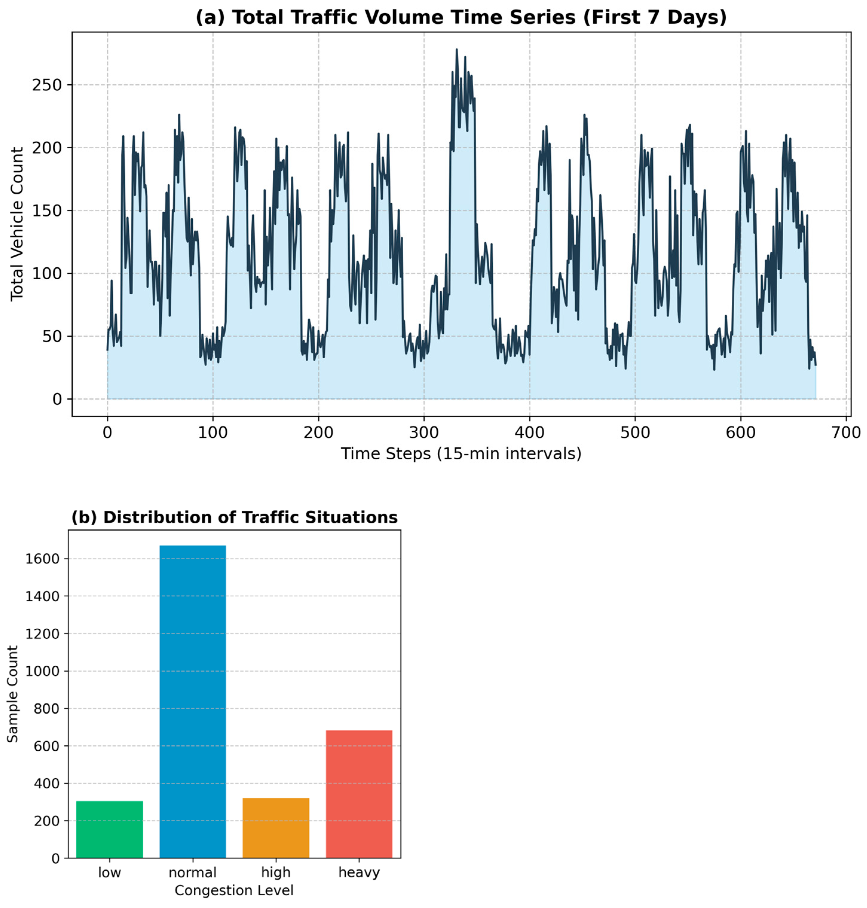
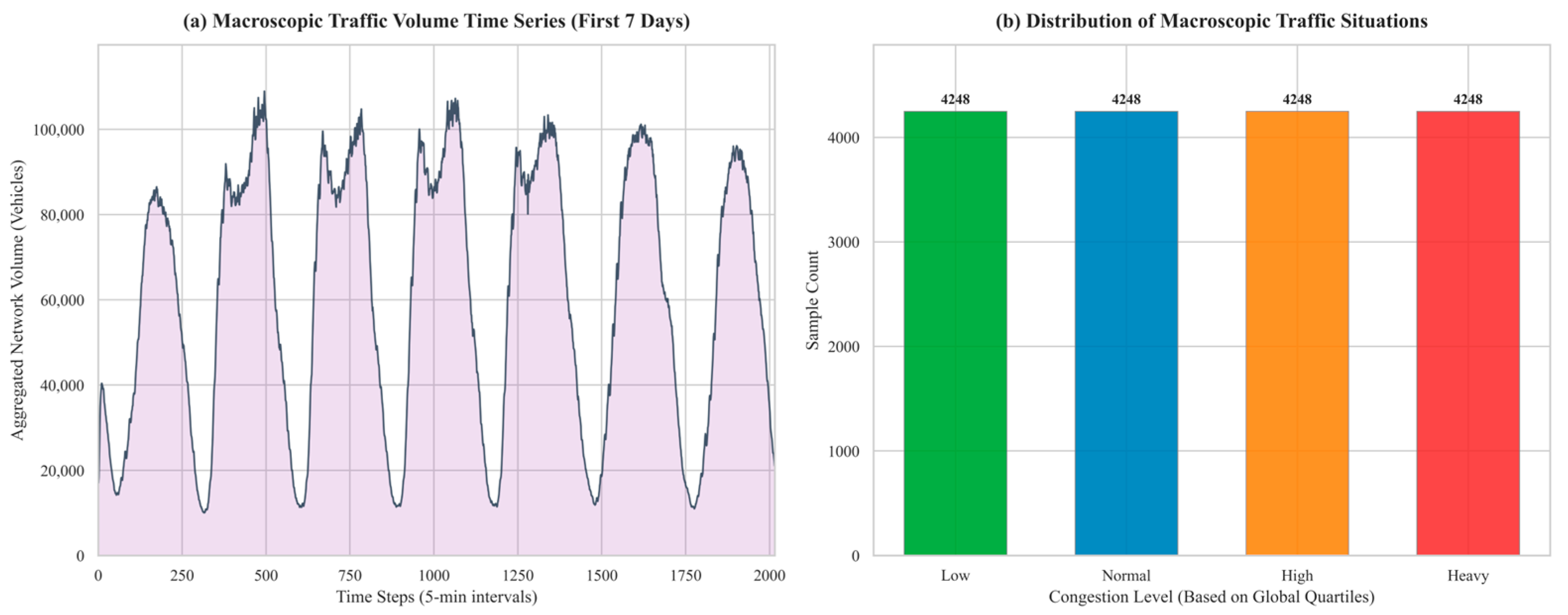
To further validate the framework’s versatility across different physical traffic metrics and larger spatial topologies, the PeMSD4 dataset is utilized as the third evaluation benchmark. Collected by the California Department of Transportation (Caltrans) Performance Measurement System (PeMS), this dataset captures highway traffic flow (volume) data in the San Francisco Bay Area. It comprises continuous measurements from 307 interconnected sensor stations spanning from 1 January 2018, to 28 February 2018. Aggregated at 5 min intervals, the temporal sequence yields a total of 16,992 observations.

Unlike the velocity-centric node-level evaluation in METR-LA, our experiment on PeMSD4 investigates macroscopic network congestion. The traffic volumes across all 307 nodes are spatially aggregated (summed) at each time step to represent the global traffic load of the regional network. Consequently, the continuous macroscopic volume is discretized into four categorical states using global statistical percentiles (25%, 50%, and 75%): Heavy, High, Normal, and Low. In this volume-based paradigm, higher traffic flow indicates a heavier congestion load on the highway network. Figure 5a depicts the macroscopic traffic volume fluctuations over the first 7 days, capturing a highly regular and periodic diurnal commuting pattern characterized by distinct daily volume peaks.

Figure 5b illustrates the sample distribution of the discretized congestion levels. Notably, due to the quartile-based thresholding strategy applied to the aggregated macroscopic volume, the PeMSD4 dataset presents a perfectly balanced class distribution, with exactly 4248 samples per category (Low, Normal, High, and Heavy). This balanced statistical characteristic starkly contrasts with the severe long-tail imbalance observed in the METR-LA dataset. Including both highly imbalanced and perfectly balanced datasets establishes a rigorous and comprehensive evaluation matrix. It verifies that the proposed IHO-CNN-BiLSTM-Attention architecture can maintain exceptional feature extraction and generalization stability regardless of the underlying statistical distribution of the data.

Consistent with the previous experimental designs, the sequential integrity of the time-series data is strictly preserved. The dataset is partitioned chronologically into training (70%), validation (10%), and testing (20%) sets, preventing any temporal data leakage.

4.2. Model Evaluation

To quantitatively assess the performance of the proposed IHO-CNN-BiLSTM-Attention model in traffic state forecasting, several standard classification metrics are employed. It is essential to emphasize that the selection of these metrics is dictated by the formulation of our problem as a four-class classification task. This framing is specifically chosen because categorical congestion levels (e.g., transitioning from ‘Normal’ to ‘Heavy’) provide more direct and actionable insights for macroscopic Intelligent Transportation Systems (ITS) management compared to minor fluctuations in continuous vehicle counts. Furthermore, the classification approach acts as a robust filter against high-frequency random noise inherent in 15 min sampling intervals, ensuring the model captures meaningful spatiotemporal state transitions.

The following metrics are utilized to evaluate the model’s accuracy, precision, and stability [32,33,34]:

$$\mathrm{Accuracy} ={\displaystyle \frac{TP+TN}{TP+TN+FP+FN}}$$

(18)

$$\mathrm{Precision}={\displaystyle \frac{TP}{TP+FP}}$$

(19)

$$\mathrm{Recall}={\displaystyle \frac{TP}{TP+FN}}$$

(20)

$$\mathrm{F}1 \mathrm{Score}={\displaystyle \frac{2\times \mathrm{Precision}\times \mathrm{Recall}}{\mathrm{Precision}+\mathrm{Recall}}}$$

(21)

In the formulas, TP represents True Positives, TN represents True Negatives, FP represents False Positives, and FN represents False Negatives. The higher the values of these metrics, the better the model’s prediction performance and accuracy.

4.3. IHO Comparison Experiment

4.3.1. Selection of Test Functions and Experimental Settings

To fully verify the performance advantages of the proposed IHO algorithm in complex high-dimensional optimization tasks, this subsection selects 9 classic benchmark test functions for testing and analysis. Among them, the fitness landscapes of unimodal functions (F1, F3, F4) are smooth and continuous within the internal area, with a unique global optimal solution and no local extreme traps, and the optimization process does not have local optimal interference; the fitness landscapes of multimodal functions (F2, F5, F6) contain a large number of widely distributed local extreme points that increase exponentially with the increase in dimensions, with intense terrain fluctuations and a concealed global optimal position; in addition, to further increase the testing difficulty, mixed functions (F7) and combined functions (F8, F9) based on the basic functions were constructed. These types of functions have highly heterogeneous fitness landscapes, containing multiple sub-optimization regions with different terrain characteristics, which can more rigorously test the algorithm’s adaptive optimization ability in complex fitness landscapes. The specific information of these 9 test functions is shown in

Table 1. Specific information of the 9 test functions.

Function Number	Function Name	Mathematical Expression	Type	Scope	Optimal Solution
F1	Sphere	${\displaystyle \sum _{i=1}^D{x}_i^2}$	Unimodal	[−100, 100]	0
F2	Rastrigin	${\displaystyle \sum _{i=1}^D\left[x_i^2-10\cos (2\pi x_i)\right]}$	Multimodal	[−5.12, 5.12]	0
F3	Schwefel 2.22	${\displaystyle {\displaystyle \sum _{i=1}^D}\Vert x_i\Vert }+{\displaystyle {\displaystyle \prod _{i=1}^D}\Vert x\Vert }$	Unimodal	[−100, 100]	0
F4	Schwefel 1.2	${\displaystyle \sum _{i=1}^D{({\displaystyle \sum _{j=1}^i{x}_j})}^2}$	Unimodal	[−100, 100]	0
F5	Schaffer N.2 (Variant)	$0.5+{\displaystyle \frac{{\sin }^2(\sqrt{{\displaystyle \sum _{i=1}^D{x}_i^2}})-0.5}{{(1+0.001{\displaystyle \sum _{i=1}^D{x}_i^2})}^2}}$	Multimodal	[−100, 100]	0
F6	Modified Penalized	${\displaystyle {\displaystyle \sum _{i=1}^D}{y}_i^2}-\cos (20\pi {\displaystyle {\displaystyle \prod _{i=1}^D}{y}_i^{1/D}})+1$	Multimodal	[−10, 10]	Dimension $D$
F7	Shifted Schwefel	$418.9829\times D-{\displaystyle \sum _{i=1}^D\left[z_i\cdot \sin (\sqrt{\left|z_i\right|})\right]}$	Hybrid	[−500, 500]	Variation
F8	Hybrid Function	${\displaystyle \frac{1}{4}}[g_1(x_1)+g_2(x_2)+g_3(x_3)+g_4(x_4)]$	Composition	[−100, 100]	$D_4/4$
F9	Composition Function	${\displaystyle \sum _{k=1}^{5}0}.2\times [F_{sub\_k}(x-O_k)+100(k-1)]$	Composition	[−100, 100]	/

.

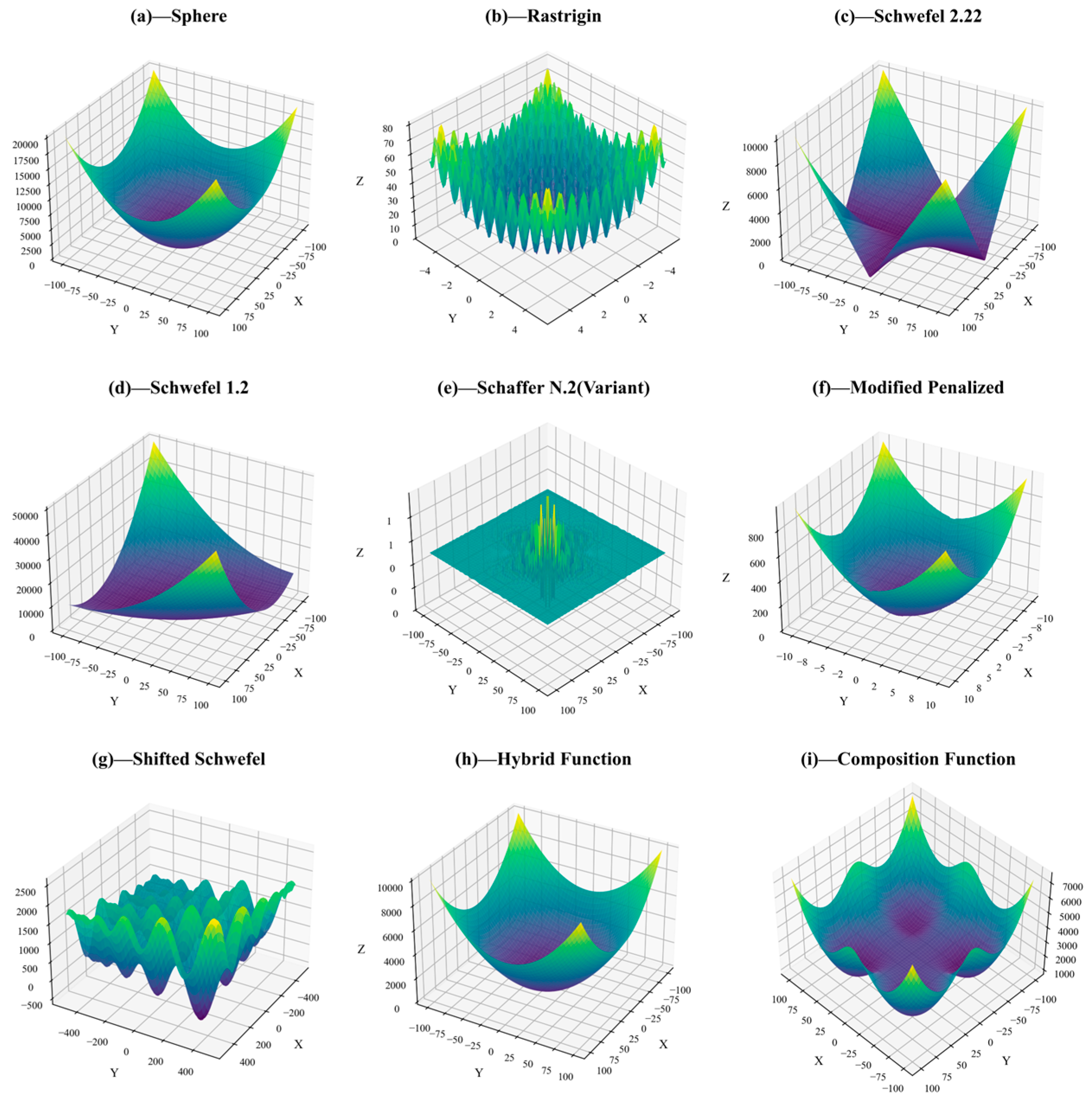
To provide an intuitive view of the fitness landscape complexity of the test functions’ search space, Figure 6 shows the 3D surface plots of the selected test functions.

4.3.2. Analysis of Optimization Accuracy and Stability

To ensure the fairness of comparative experiments and the statistical significance of the results, and to eliminate systematic interference of extraneous variables on the conclusions, this study selects representative metaheuristic algorithms with distinct design logics for cross-comparison. The selected algorithms include: the classic swarm intelligence algorithm Grey Wolf Optimizer (GWO) [35], the mainstream high-performance Sparrow Search Algorithm (SSA) [36], and two newly proposed metaheuristic algorithms, namely the Parrot Optimization Algorithm (POA) [37] and the Crested Porcupine Optimization (CPO) [38]. Meanwhile, the original Hippopotamus Optimization Algorithm is included as the control baseline.

All experiments are conducted on 9 classic benchmark test functions with a dimension of 30. For each compared algorithm, the population size is uniformly set to 30 individuals, and the maximum number of iterations is set to 500. To mitigate random errors caused by the stochastic nature of metaheuristics, each experiment is independently repeated 30 times. The mean and standard deviation (Std) derived from these independent runs are analyzed in depth to characterize the comprehensive performance of IHO in terms of optimization accuracy and numerical stability. The detailed statistical results of the 30-dimensional experiments are presented in

Table 2. 30-dimensional experimental results.

Function	Indicators	GWO	SSA	POA	CPO	HO	IHO
F1	Mean	2.42 × 10−72	5.60 × 10−28	3.78 × 101	1.76 × 102	3.58 × 102	1.42 × 10−228
	Std	1.26 × 10−71	3.01 × 10−27	1.20 × 101	1.99 × 102	1.04 × 102	0.00 × 100
F2	Mean	0.00 × 100	4.33 × 10−9	1.03 × 102	7.80 × 101	2.27 × 102	0.00 × 100
	Std	0.00 × 100	2.24 × 10−8	2.00 × 101	2.31 × 101	4.67 × 101	0.00 × 100
F3	Mean	1.22 × 10−45	1.28 × 10−13	5.97 × 102	3.72 × 102	3.21 × 1034	6.27 × 10−119
	Std	2.37 × 10−45	6.82 × 10−13	1.15 × 102	1.56 × 102	1.43 × 1035	3.37 × 10−118
F4	Mean	1.40 × 10−4	1.02 × 10−37	2.52 × 103	2.05 × 103	1.23 × 104	9.67 × 10−131
	Std	4.08 × 10−4	5.48 × 10−37	9.28 × 102	9.03 × 102	3.59 × 103	3.54 × 10−130
F5	Mean	3.89 × 10−3	0.00 × 100	3.75 × 10−1	4.75 × 10−1	4.68 × 10−1	2.91 × 10−3
	Std	4.76 × 10−3	0.00 × 100	4.37 × 10−2	1.46 × 10−2	2.03 × 10−2	4.45 × 10−3
F6	Mean	3.00 × 101	3.00 × 101	5.51 × 101	3.00 × 101	1.33 × 102	3.00 × 101
	Std	0.00 × 100	0.00 × 100	2.95 × 101	0.00 × 100	3.05 × 101	0.00 × 100
F7	Mean	−6.60 × 102	−2.84 × 101	−5.00 × 102	−9.42 × 102	8.64 × 102	−3.90 × 103
	Std	1.43 × 103	7.34 × 101	1.10 × 103	1.14 × 103	1.04 × 103	2.94 × 103
F8	Mean	2.00 × 100	2.00 × 100	5.13 × 101	3.48 × 101	5.95 × 101	2.00 × 100
	Std	0.00 × 100	6.28 × 10−5	1.74 × 101	3.20 × 101	1.89 × 101	0.00 × 100
F9	Mean	3.83 × 102	3.60 × 102	2.04 × 103	4.84 × 103	3.17 × 104	3.50 × 102
	Std	8.62 × 100	5.09 × 100	2.69 × 103	3.18 × 103	1.98 × 104	4.28 × 100

.

The mean optimization value and standard deviation are adopted as the core evaluation indicators in the above two tables, and the bold values in the tables represent the optimal solutions of the corresponding functions. It is found that the Improved Hippo Optimization Algorithm (IHO) delivers the optimal comprehensive performance on nine classical benchmark test functions with no obvious degradation in performance advantages, demonstrating excellent high-dimensional space adaptability and optimization robustness. The detailed performances are analyzed as follows:

• Unimodal functions feature a smooth internal fitness landscape, and are mainly used to evaluate the local exploitation accuracy and vertical convergence speed of optimization algorithms. The optimization accuracy of IHO on F1, F3 and F4 is several orders of magnitude higher than that of other comparison algorithms, maintaining high solution accuracy, strong dimensional scalability and superior approximation capability to the single global optimal solution.
• Multimodal functions contain a large number of local optimal traps, which severely test the algorithm’s ability to escape local optima. For the classical multimodal function F2, IHO converges to the theoretical optimal value with a standard deviation of 0 under 30 dimensions. In addition, for F6 with a penalty mechanism, IHO accurately reaches its mathematical lower bound at 30 dimensions while maintaining a constant standard deviation of 0, showing outstanding performance in breaking away from local optimum stagnation.
• These two types of functions are characterized by high randomness and extremely high optimization difficulty. In terms of F8 and F9, IHO outperforms or is comparable to other algorithms in both mean value and standard deviation. This indicates that the multi-strategy collaboration mechanism effectively enhances the overall optimization robustness of the algorithm in unknown, complex and variable environments.

4.3.3. Convergence Analysis

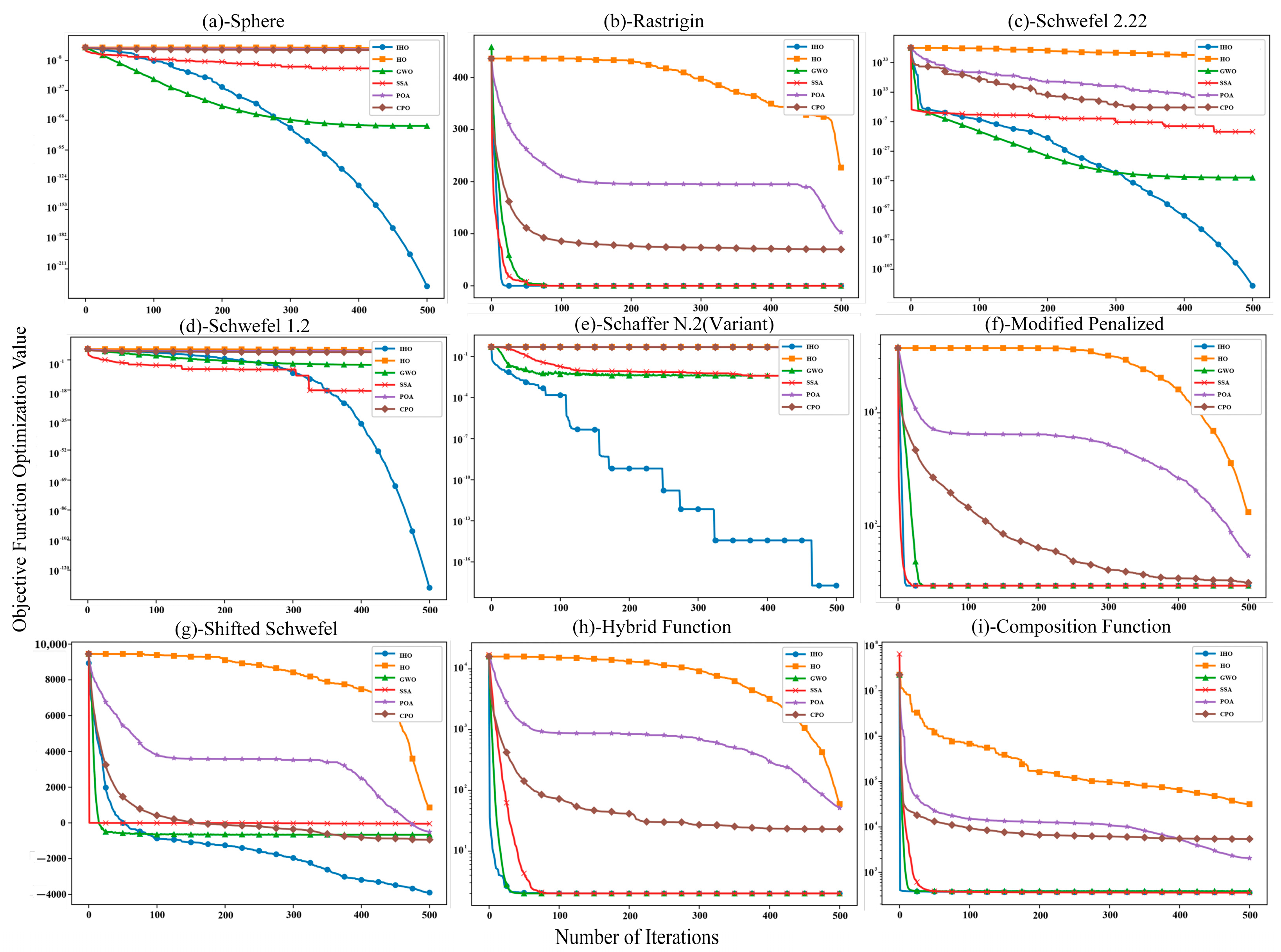
Convergence is one of the core evaluation indicators of metaheuristic optimization algorithms. It intuitively reflects the algorithm’s balance capability between global exploration and local exploitation, optimization efficiency, and global convergence potential. Superior convergence performance enables the algorithm to quickly approach the optimal solution and avoid problems such as premature stagnation and low solution accuracy. Convergence analysis can reveal the optimization mechanism of the algorithm and verify the effectiveness of the improved strategy. In this study, the average convergence curves of six algorithms obtained from 30 independent experiments on nine benchmark functions are plotted to analyze the convergence speed and optimization effect of IHO. As shown in Figure 7:

Based on the average convergence curves of nine classical 30-dimensional benchmark functions, the dynamic optimization performance of IHO and other five algorithms is compared and analyzed as follows:

• These functions are adopted to test the local exploitation capability and convergence accuracy. IHO possesses excellent deep mining ability. It achieves stable convergence throughout the iteration on F1 and F3, with its accuracy far exceeding other algorithms. On F4, IHO converges rapidly in a cliff-like trend after early exploration and approaches the optimal fitness value. By contrast, GWO and SSA are prone to iteration stagnation, and the original HO shows poor convergence performance.
• Such functions focus on testing the algorithm’s capability to escape local optima. IHO, GWO and SSA all achieve fast convergence in the early stage on F2 and F6. On F5, all comparison algorithms fall into high-value stagnation prematurely, while IHO presents a stepwise downward trend, which enables it to escape local optima repeatedly and continuously approach the global optimum.
• With complex search spaces, these functions can effectively verify the comprehensive optimization capability of algorithms. Only IHO maintains continuous optimization ability on F7. For F8 and F9, IHO features a smoother convergence curve and faster initial convergence speed with better stability.

In conclusion, in the 30-dimensional complex search space, IHO significantly outperforms the comparison algorithms in deep optimization of unimodal functions, local optimum escape of multimodal functions, and stable convergence of complex functions. The results effectively verify the feasibility and superiority of the improved strategy proposed in this paper.

4.3.4. Wilcoxon Rank-Sum Test

To further statistically verify the significance of performance differences between IHO and the comparison algorithms, address the limitations of descriptive statistics (e.g., mean and standard deviation) in statistical inference, and comprehensively quantify the actual performance gaps, the Wilcoxon rank-sum test is adopted to analyze the experimental results of each algorithm over 30 independent runs. The significance level is set to α = 0.05. As a non-parametric test method, the Wilcoxon rank-sum test does not require samples to follow a normal distribution. It is suitable for comparing differences in multiple independent runs of metaheuristic optimization algorithms, effectively avoiding analysis biases caused by the normality assumption, and enabling an objective assessment of whether there are statistically significant differences between the improved algorithm and the comparison algorithms.

The test criteria are as follows: If p < 0.05, the null hypothesis is rejected, indicating a statistically significant difference in performance between IHO and the corresponding comparison algorithm on the test function; if p ≥ 0.05, the difference between the two algorithms on the function is considered not statistically significant. The Wilcoxon rank-sum test results of IHO and the comparison algorithms in the 100-dimensional environment are presented in

Table 3. The results of the Wilcoxon rank sum test in a 100-dimensional environment (“*” in the table indicates a significant difference between IHO).

Function	IHO vs. GWO	IHO vs. SSA	IHO vs. POA	IHO vs. CPO	IHO vs. HO
F1	<0.0001 *	<0.0001 *	<0.0001 *	<0.0001 *	<0.0001 *
F2	0.5000	0.3639	<0.0001 *	<0.0001 *	<0.0001 *
F3	<0.0001 *	0.0005 *	<0.0001 *	<0.0001 *	<0.0001 *
F4	<0.0001 *	<0.0001 *	<0.0001 *	<0.0001 *	<0.0001 *
F5	0.7559	0.9995	<0.0001 *	<0.0001 *	<0.0001 *
F6	0.5000	0.5000	<0.0001 *	<0.0001 *	<0.0001 *
F7	0.0526	0.0003 *	<0.0001 *	<0.0001 *	<0.0001 *
F8	0.5000	0.1011	<0.0001 *	<0.0001 *	<0.0001 *
F9	<0.0001 *	<0.0001 *	<0.0001 *	<0.0001 *	<0.0001 *

.

The results in Table 3 show that IHO exhibits significant statistical superiority over most comparison algorithms in the 100-dimensional high-complexity search space. The extremely small p-values on multiple test functions indicate that the performance differences are not caused by random fluctuations but have clear statistical significance. The detailed analysis is as follows:

• Comparison with the original HO and novel algorithms POA, CPO: The p-values on all 9 test functions are less than 0.05, indicating statistically significant differences in the distribution of results between IHO and the above algorithms across all functions. IHO achieves stable and significant performance improvements in high-dimensional complex optimization scenarios.
• Comparison with the classic algorithm GWO: IHO shows significant differences with GWO on F1, F3, F4 and F9 (p < 0.05). On F2, F6 and F8, the p-value is 0.5000, as both algorithms converge to the theoretical global optimal value at this dimension with zero variance of objective function values, demonstrating equivalent convergence capability. On F5 and F7, the p-value is slightly greater than 0.05, indicating comparable performance between the two algorithms.
• Comparison with the mainstream algorithm SSA: Significant differences are observed between IHO and SSA on F1, F3, F4, F7 and F9 (p < 0.05). Both algorithms converge to the theoretical global optimal value on F6, while no statistically significant differences exist on F2, F5 and F8.

In conclusion, for 100-dimensional high-complexity optimization problems, IHO shows statistically significant differences from HO, POA and CPO on all test functions; it outperforms GWO and SSA significantly on most functions and performs comparably on a few. Overall, IHO exhibits notable statistical advantages and strong robustness in high-dimensional complex environments, providing further data support for its anti-dimensionality curse capability.

4.3.5. IHO Ablation Experiment

To quantitatively evaluate the marginal contribution of each improved module in the IHO algorithm, this study adopts an incremental addition strategy. On the basis of the standard HO, four major improved modules are introduced sequentially, and five different algorithm configurations are constructed under identical experimental conditions (population size, maximum iterations, problem dimension, number of independent runs, and hardware/software environment):

• Configuration A (HO): The original Hippo Optimization Algorithm, serving as the performance baseline.
• Configuration B (HO-I): HO with the addition of the piecewise linear chaotic mapping topological reconstruction module.
• Configuration C (HO-II): HO-I with the addition of the nonlinear adaptive inertia weight module.
• Configuration D (HO-III): HO-II with the addition of the tangent flight defense mechanism module.
• Configuration E (IHO): The complete configuration, which integrates the lens imaging opposition-based learning post-processing module into HO-III.

All experiments are conducted with the same parameter settings: population size $N=30$, dimension $D=30$, and maximum number of iterations $T=500$. To comprehensively investigate the performance of the improved modules under different function characteristics, unimodal functions (F1, F3), multimodal function (F6), and composite function (F9) are selected as test benchmarks. Each configuration runs independently 30 times on the benchmark functions, and the mean and standard deviation of the convergence results are recorded, aiming to comprehensively evaluate the performance of IHO from both accuracy and stability perspectives.

The ablation experiment results in

Table 4. Summary of improved module ablation experiment results.

Function	A (HO)	B (HO-I)	C (HO-II)	D (HO-III)	E (IHO)
F1	3.58 × 102 ± 1.04 × 102	1.25 × 101 ± 2.31 × 100	4.31 × 10−12 ± 1.05 × 10−12	8.94 × 10−56 ± 2.14 × 10−57	1.42 × 10−228 ± 0.00 × 100
F3	3.21 × 1034 ± 1.43 × 1035	8.94 × 1012 ± 4.12 × 1012	1.54 × 10−30 ± 2.11 × 10−31	4.12 × 10−85 ± 5.33 × 10−86	6.27 × 10−119 ± 3.37 × 10−118
F6	1.33 × 102 ± 3.05 × 101	8.52 × 101 ± 1.42 × 101	6.44 × 101 ± 9.23 × 100	3.00 × 101 ± 0.00 × 100	3.00 × 101 ± 0.00 × 100
F9	3.17 × 104 ± 1.98 × 104	1.42 × 104 ± 5.21 × 103	8.95 × 103 ± 1.04 × 103	6.12 × 102 ± 9.54 × 101	3.50 × 102 ± 4.28 × 100

verify the effectiveness and synergistic effect of each improved module. With the sequential introduction of modules, the algorithm’s convergence accuracy and stability continue to improve across different test functions. The marginal contribution of each module is analyzed as follows:

• Piecewise Chaotic Mapping Initialization (HO vs. HO-I): This module addresses population clustering caused by pseudo-random initialization, improves initial solution space coverage, and optimizes global exploration capability. Consequently, HO-I outperforms the original HO on all test functions.
• Nonlinear Adaptive Inertia Weight (HO-I vs. HO-II): It achieves a smooth transition between early-iteration exploration and late-iteration exploitation via tangent transformation, optimizing the exploration–exploitation balance. HO-II’s convergence accuracy improves by several orders of magnitude on unimodal functions F1 and F3.
• Tangent Flight Defense Mechanism (HO-II vs. HO-III): By replacing the original Lévy flight with controllable step sizes, this module retains global breakthrough capability while avoiding search oscillations, enhancing local optimum escape ability. As a result, HO-III converges to the theoretical optimal value on multimodal function F6, with significantly improved performance on composite function F9.
• Lens Imaging Opposition-Based Learning (HO-III vs. IHO): At the end of iterations, this module generates conjugate opposite solutions based on the current optimal solution, expanding the search range and avoiding premature convergence. The complete IHO achieves the best performance on all test functions, with further optimized accuracy and stability especially on the most complex composite function F9.

In summary, the four improvements targetedly optimize the original HO from four dimensions: population initialization, exploration–exploitation balance, local optimum escape, and premature convergence avoidance, forming a complementary synergistic effect between modules. The ablation experiment fully verifies the effectiveness of each improved strategy, proving that IHO’s performance improvement stems from multi-module collaborative optimization, providing a reliable basis for its application in engineering optimization tasks.

4.3.6. Comparative Modelling Experiments of Different Optimization Algorithms

To deeply explore the impact of both model architecture design and optimization algorithm selection on traffic prediction performance, we conducted comprehensive comparative experiments on the multi-modal intersection dataset. The evaluation metrics include Accuracy, Precision, Recall, and F1-Score, with detailed results presented in

Table 5. Comparative experiments of different optimization algorithms in the model (bolded text indicates the best option).

Data	Model	Accuracy	Precision	Recall	F1 Score
Traffic	IHO-LSTM-	0.9571	0.9559	0.9498	0.9538
Traffic	IHO-BiLSTM	0.9611	0.9624	0.9521	0.9587
Traffic	IHO-CNN-BiLSTM	0.9653	0.9489	0.9578	0.9598
Traffic	IHO-ASTformer	0.9544	0.9439	0.9568	0.9577
Traffic	IHO-DiffSTG	0.9678	0.9633	0.9609	0.9612
Traffic	PSO-CNN-BiLSTM-Attention	0.9781	0.9559	0.9547	0.9543
Traffic	GWO-CNN-BiLSTM-Attention	0.9782	0.9330	0.9279	0.9281
Traffic	SSA-CNN-BiLSTM-Attention	0.9715	0.9345	0.9262	0.9275
Traffic	WOA-CNN-BiLSTM-Attention	0.9748	0.9491	0.9463	0.9465
Traffic	HO-CNN-BiLSTM-Attention	0.9664	0.9663	0.9664	0.9661
Traffic	IHO-CNN-BiLSTM-Attention	0.9798	0.9799	0.9799	0.9798

.

As shown in the Table, the comparative analysis is divided into three key aspects:

• Architectural Evolution under IHO Optimization: We evaluated the baseline architectures (LSTM, BiLSTM, CNN-BiLSTM) uniformly optimized by the proposed IHO algorithm. ‘IHO-LSTM’ and ‘IHO-BiLSTM’ achieve baseline F1-Scores of 0.9538 and 0.9587, respectively. Integrating CNN for spatial feature extraction (‘IHO-CNN-BiLSTM’) lifts the F1-Score to 0.9598. Ultimately, the full ‘IHO-CNN-BiLSTM-Attention’ architecture achieves a peak F1-Score of 0.9798. This progression proves that the sequential addition of spatial, temporal, and attention modules steadily enhances predictive capability when properly tuned.
• IHO Applied to Contemporary SOTA Architectures: To verify the generalizability of the IHO algorithm and compare architectural suitability, we applied it to the latest generative and attention-heavy models, resulting in ‘IHO-ASTformer’ and ‘IHO-DiffSTG’. While IHO successfully optimizes these heavy networks to achieve highly competitive F1-Scores of 0.9577 and 0.9612, they still fall short of the 0.9798 achieved by our proposed architecture. This demonstrates that while contemporary SOTA models are powerful, our lightweight CNN-BiLSTM-Attention structure is fundamentally more suitable and efficient for handling the localized spatiotemporal features of urban traffic data.
• Optimizer Comparison on the Proposed Framework: Building on the CNN-BiLSTM-Attention architecture, we further compare different optimization algorithms. Traditional optimizers (PSO, GWO, SSA, WOA) achieve relatively high overall Accuracy (0.9715–0.9782), but suffer from severe performance imbalance: GWO and SSA yield the lowest F1-Scores (0.9281 and 0.9275, respectively), indicating poor generalization to complex minority traffic states due to premature convergence. The original HO algorithm alleviates this imbalance (F1-Score 0.9661) but fails to surpass the Accuracy of traditional optimizers. In stark contrast, the proposed IHO algorithm delivers consistent, state-of-the-art performance across all metrics (Accuracy and F1-Score at 0.9798), outperforming all other optimizers by a clear margin.

In contrast, the proposed IHO algorithm delivers consistent, state-of-the-art performance across all metrics. The final IHO-CNN-BiLSTM-Attention model achieves an Accuracy, Precision, Recall, and F1-Score all around 0.9798, outperforming all other models by a clear margin. This confirms that for 15 min granular traffic data, the explicit extraction of local spatial features (CNN) combined with progressive temporal modeling (BiLSTM) and IHO-tuned attention remains the most effective structural and optimization strategy.

4.4. Comparative Experiments and Analysis

4.4.1. Performance on Intersectional Dataset

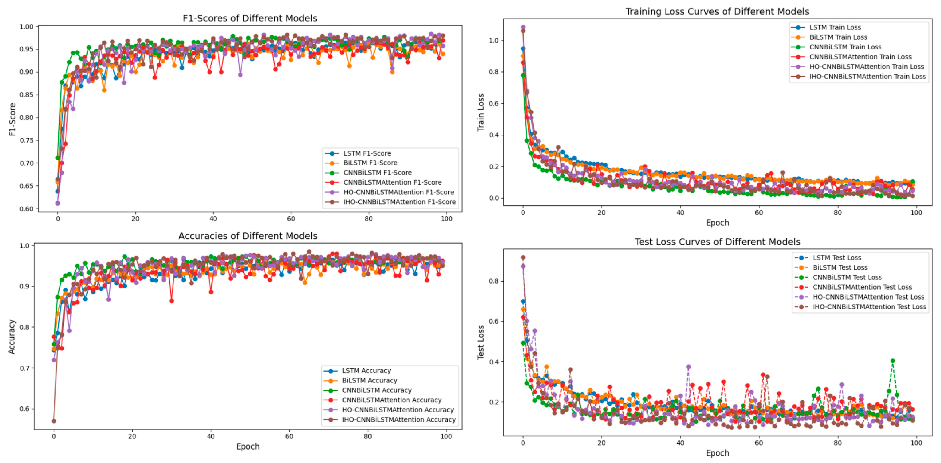
To validate the performance of the IHO-CNN-BiLSTM-Attention traffic flow prediction model, this study selects LSTM, BiLSTM, CNN-BiLSTM, CNN-BiLSTM-Attention, and HO-CNN-BiLSTM-Attention models for comparison experiments. To reduce the impact of training variability, multiple training runs are performed for each model, and the optimal results are recorded. The specific data is shown in

Table 6. Experimental results of different model comparisons (bolded text indicates the best option).

Data	Model	Accuracy	Precision	Recall	F1 Score
Traffic	LSTM	0.9430	0.9487	0.9463	0.9465
Traffic	BiLSTM	0.9396	0.9413	0.9379	0.9368
Traffic	CNN-BiLSTM	0.9698	0.9704	0.9698	0.9698
Traffic	CNN-BiLSTM-Attention	0.9480	0.9503	0.9480	0.9480
Traffic	HO-CNN-BiLSTM-Attention	0.9664	0.9663	0.9664	0.9661
Traffic	IHO-CNN-BiLSTM-Attention	0.9798	0.9799	0.9799	0.9798

, and the comparisons of F1-Score, accuracy, and loss function are shown in Figure 8.

A comprehensive analysis of the charts indicates that the IHO-CNN-BiLSTM-Attention model demonstrates significant advantages across all evaluation metrics. The detailed analysis is as follows: Among the baseline models, the single-module LSTM and BiLSTM struggle to fully capture the spatiotemporal characteristics of traffic data, with accuracies of 0.9430 and 0.9396, respectively. After introducing CNN for spatial feature extraction, the accuracy of CNN-BiLSTM improves to 0.9698. However, the model with an added attention mechanism but without hyperparameter optimization experiences a performance decline, with accuracy dropping to 0.9480. In contrast, after optimization using the HO and IHO algorithms, the accuracy stabilizes at 0.9664 and is further enhanced to 0.9798, respectively. Moreover, precision, recall, and F1-score all approach 0.9799, demonstrating the effectiveness of the optimization algorithms. From the perspective of the loss function, the test loss of the proposed model eventually stabilizes around 0.2, which is lower than that of the comparison models. Its training loss converges faster and to a lower value, indicating superior generalization capability and training stability.

4.4.2. Generalization Analysis on METR-LA

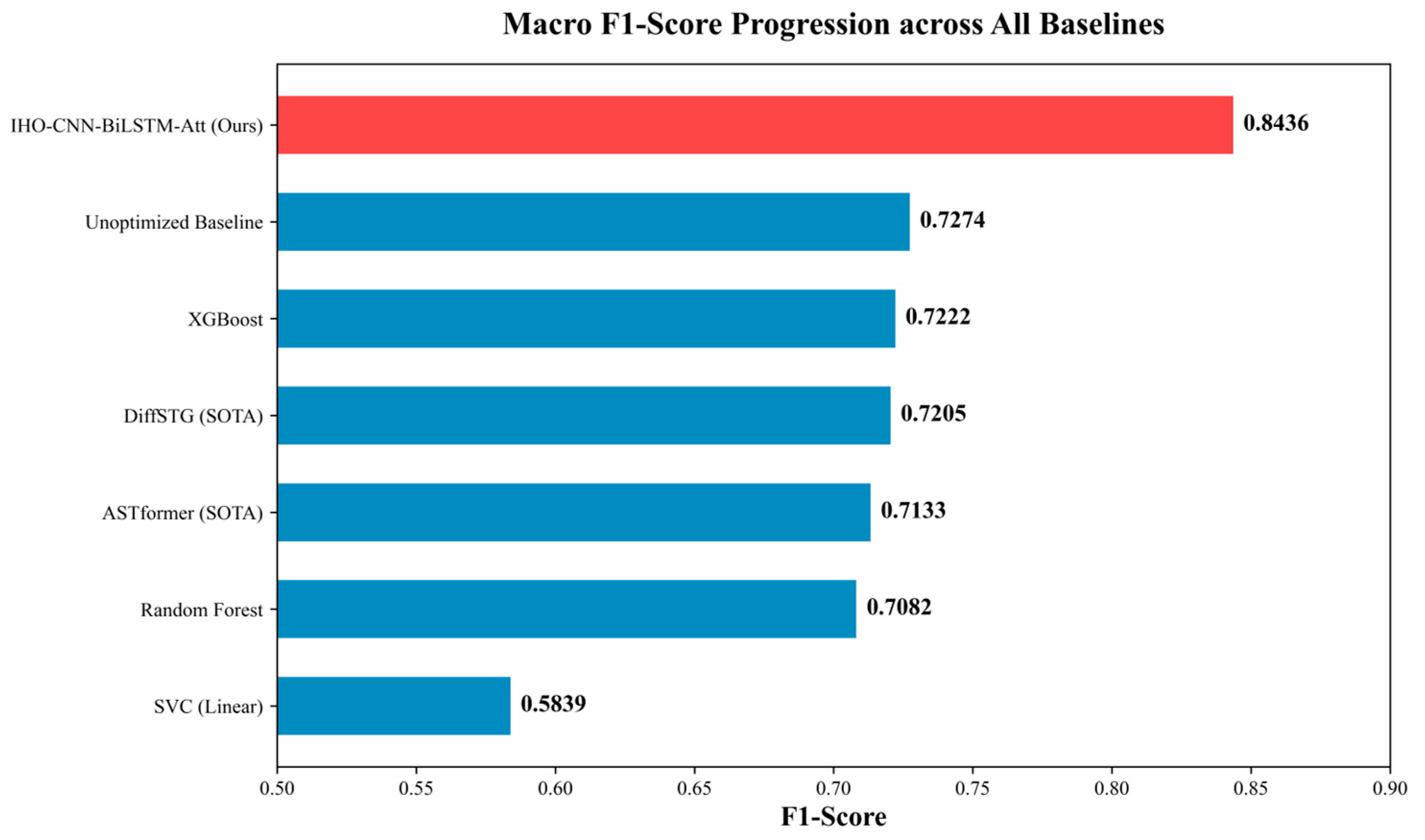
To rigorously validate the generalization capability of the proposed architecture under severe long-tail data distributions, a comprehensive comparative analysis was conducted on the METR-LA dataset. We evaluated the proposed framework alongside two tiers of baselines: classical machine learning ensembles (SVC, Random Forest, XGBoost) and contemporary state-of-the-art (SOTA) deep learning architectures (Attention-based Spatio-Temporal Transformer [ASTformer] and Diffusion-based Spatio-Temporal Classifier [DiffSTG]). The quantitative results are detailed in

Table 7. Performance comparison of different models on the METR-LA dataset (bolded text indicates the best option).

Model Tier	Model	Accuracy	Precision	Recall	F1 Score
Classical ML	SVC (Linear)	0.7615	0.5598	0.6348	0.5839
	Random Forest	0.9406	0.7073	0.7092	0.7082
	XGBoost	0.9508	0.9646	0.7191	0.7222
Deep Learning	Unoptimized Baseline	0.9602	0.8431	0.7262	0.7274
	ASTformer (SOTA)	0.9546	0.7117	0.7149	0.7133
	DiffSTG (SOTA)	0.9616	0.7215	0.7198	0.7205
Proposed	IHO-CNN-BiLSTM-Attention (Ours)	0.9591	0.8798	0.8177	0.8436

.

The experimental results provide a compelling insight into macroscopic traffic state prediction. As demonstrated in Table 7, classical machine learning algorithms struggle significantly with this task. Specifically, flattening the spatiotemporal matrices into 1D arrays for linear models like SVC completely destroys the inherent graph topology, resulting in a failure to converge effectively (F1-Score: 0.5839). While tree-based ensemble methods such as XGBoost achieve a high overall Accuracy (0.9508), their macro F1-Score plateaus at 0.7222. This underperformance stems from their inability to capture deep localized spatial dependencies.

Furthermore, the evaluation exposes a critical vulnerability in contemporary SOTA architectures. Although both ASTformer and DiffSTG achieve excellent global Accuracy (up to 0.9616), they severely underperform in the macro F1-Score (0.7133 and 0.7205, respectively), as visually emphasized in the leaderboard progression (Figure 9). This discrepancy occurs because heavy generative and transformer-based architectures inherently possess massive parameter spaces. Without rigorous, instance-specific hyperparameter tuning, these models tend to overfit the majority class (e.g., free-flow conditions) in highly imbalanced datasets like METR-LA, failing to accurately recall minority anomalies such as severe congestion.

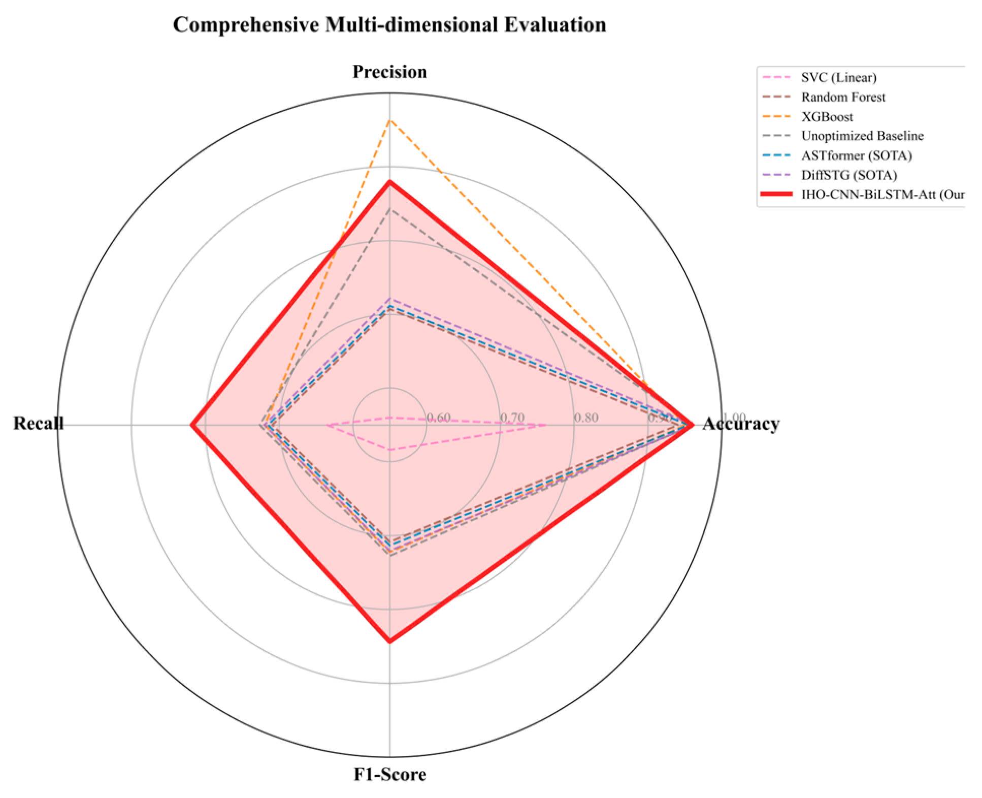
In stark contrast, the proposed IHO-CNN-BiLSTM-Attention framework fundamentally overcomes this bottleneck. As illustrated in the multi-dimensional radar chart (Figure 10), our model robustly wraps around all other baselines, exhibiting no performance trade-offs. By leveraging the Improved Hippopotamus Optimization algorithm to autonomously navigate the hyperparameter space, the network precisely balances its structural capacity. It achieves the highest F1-Score of 0.8436—outperforming all SOTA baselines by a significant margin of over 12%. This robustly validates that dynamically optimizing a lightweight CNN-BiLSTM architecture is a significantly more effective and reliable strategy for handling imbalanced macroscopic traffic data than merely deploying unoptimized, parameter-heavy SOTA models.

4.4.3. Generalization Analysis on PeMSD4

To further evaluate the model’s adaptability to a fundamentally different data distribution—specifically, a perfectly balanced, macroscopic volume-based dataset—a parallel comparative analysis was conducted on the PeMSD4 dataset. Identical to the previous experiment, the proposed framework was benchmarked against classical machine learning algorithms and contemporary SOTA deep spatiotemporal models. The comprehensive quantitative results are summarized in

Table 8. Performance comparison of different models on the PeMSD4 dataset (bolded text indicates the best option).

Model Tier	Model	Accuracy	Precision	Recall	F1 Score
Classical ML	SVC (Linear)	0.8425	0.8379	0.8426	0.8389
	Random Forest	0.9502	0.9490	0.9525	0.9500
	XGBoost	0.9320	0.9361	0.9277	0.9301
Deep Learning	Unoptimized Baseline	0.9120	0.9235	0.9029	0.9078
	ASTformer (SOTA)	0.9223	0.9213	0.9239	0.9216
	DiffSTG (SOTA)	0.9296	0.9325	0.9252	0.9279
Proposed	IHO-CNN-BiLSTM-Attention (Ours)	0.9564	0.9550	0.9583	0.9561

.

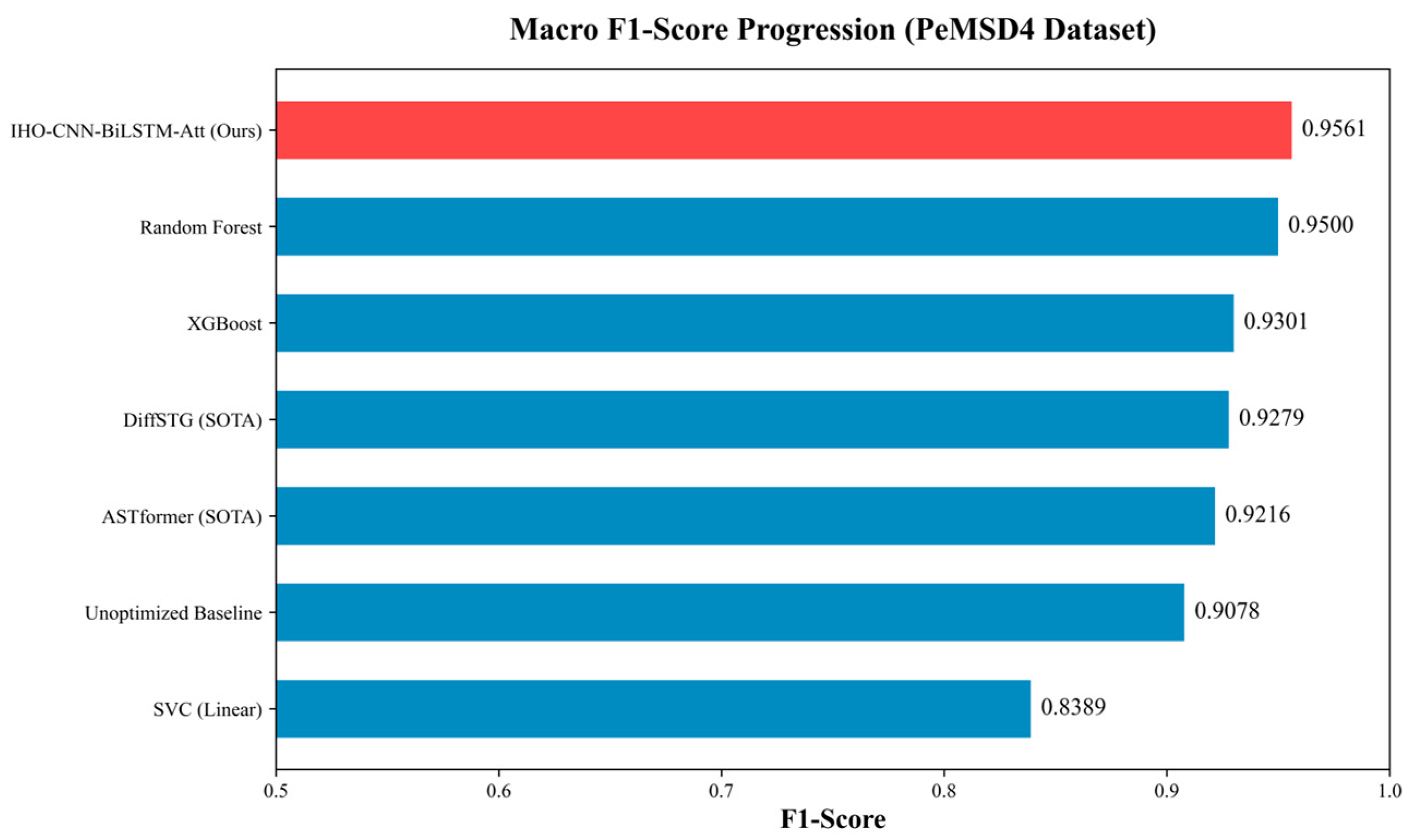
The empirical results on the PeMSD4 dataset provide a critical and objective insight into macroscopic traffic state classification. As shown in Table 8 and visually reinforced by the leaderboard (Figure 11), traditional tree-based ensemble methods—particularly Random Forest (F1-Score: 0.9500)—demonstrate highly competitive performance, significantly rebounding from their poor results on the METR-LA dataset. This phenomenon aligns with the mathematical nature of the data preprocessing: aggregating complex multi-node traffic volumes into a singular, flattened 1D temporal array inherently strips away intricate spatial graph topologies. By reducing the spatiotemporal problem to a purely tabular statistical mapping with perfectly balanced classes, tree-based ensembles are positioned to maximize their objective functions efficiently.

Conversely, the performance of contemporary heavy architectures (ASTformer and DiffSTG) degrades in this specific context, yielding F1-Scores of 0.9216 and 0.9279, respectively. When rich spatial topologies are macroscopically aggregated, the massive parameter spaces of Transformers and Diffusion models become redundant, leading to suboptimal feature extraction and hyperparameter collapse without rigorous dataset-specific tuning.

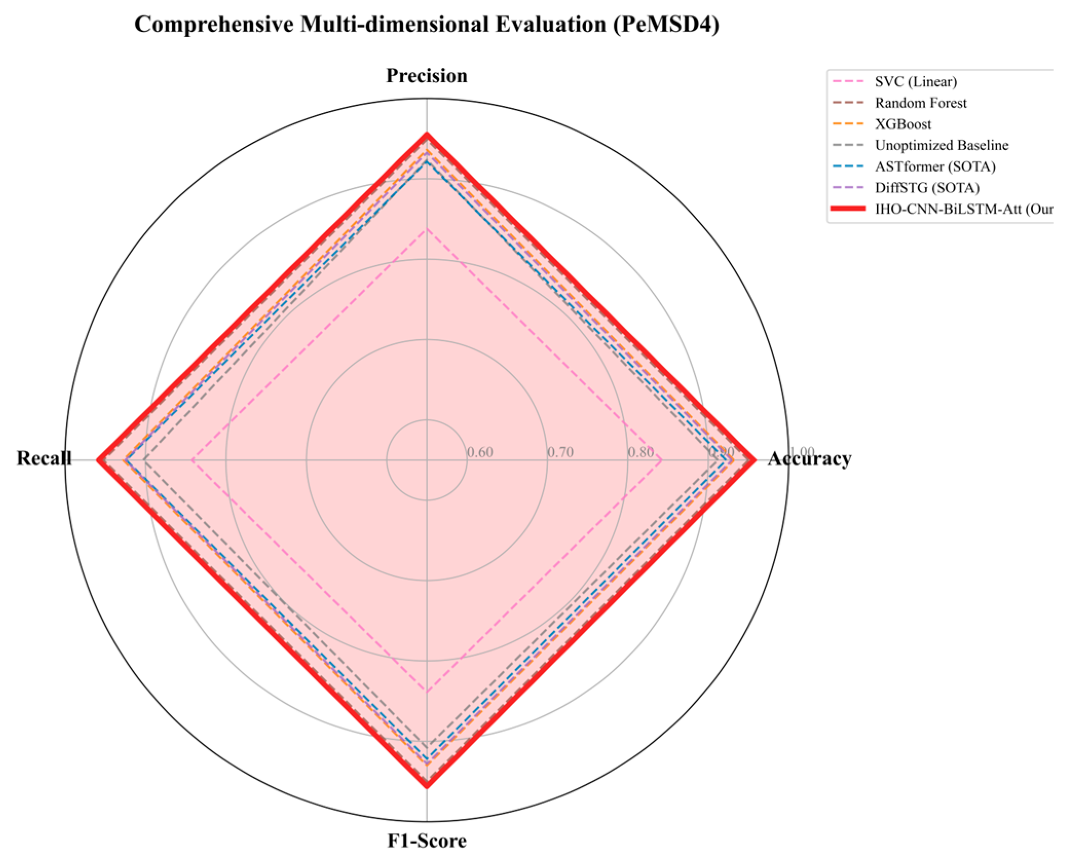
Despite these flattened data characteristics, the architectural superiority of our proposed framework is definitively validated. As depicted in the multi-dimensional radar chart (Figure 12), the IHO-CNN-BiLSTM-Attention model comprehensively dominates all evaluation metrics, achieving a peak F1-Score of 0.9561. This decisively proves the mathematical efficacy of the Chaotic-Lens Adaptive Tangent Hippopotamus Optimization (CLAT-HOA). By enabling the network to autonomously restructure its hyperparameter space specifically for the 307-node volume topology, the IHO algorithm prevents the CNN-BiLSTM from overfitting or experiencing parameter redundancy. Consequently, the proposed framework maintains exceptional robustness and state-of-the-art predictive accuracy across fundamentally diverse real-world traffic environments—mastering both severely imbalanced microscopic velocity data and perfectly balanced macroscopic volume data.

5. Conclusions

This study proposed a robust hybrid framework based on Convolutional Neural Networks (CNN), Bidirectional Long Short-Term Memory Networks (BiLSTM), and an Attention Mechanism, coupled with an Improved Hippopotamus Optimization (IHO) algorithm to boost the accuracy of short-term traffic state classification. Extensive validations on standard CEC benchmark functions proved that the integration of PWLCM, Tangent Flight, and LOBL mechanisms grants IHO exceptional capability to escape local optima and maintain optimization stability in high-dimensional spaces. Furthermore, comprehensive experimental results across three diverse real-world traffic datasets (a multimodal intersection, METR-LA, and PeMSD4) demonstrated the exceptional generalization capability of the IHO-CNN-BiLSTM-Attention model. By effectively handling both severe long-tail class imbalances and varying macroscopic physical metrics (velocity vs. volume), the proposed model consistently achieved peak F1-Scores. It successfully and decisively outperformed unoptimized contemporary heavy deep learning architectures (including ASTformer and DiffSTG), as well as models optimized by traditional meta-heuristic algorithms (PSO, GWO, SSA, WOA). This rigorously verifies the critical necessity of tailored hyperparameter optimization in complex spatiotemporal forecasting, proving that our framework can maintain state-of-the-art predictive accuracy and structural robustness across fundamentally diverse traffic environments.

Nevertheless, this study has some limitations. First, the model training process requires significant computational resources, which may impact the efficiency of practical applications. Second, although the IHO-CNN-BiLSTM-Attention model performs well in hyperparameter optimization, it does not consider the dynamic changes in real-time data. Future research can explore other methods to improve the optimization algorithm to adapt to dynamic data and reduce computational burdens through model lightweighting. Additionally, this study does not fully explore the integration of multimodal data. In the future, other related data sources (e.g., weather, holidays) can be incorporated to further enhance the model’s generalization capability and prediction accuracy. Future research can delve into the following directions: (1) Developing online learning models with adaptability and real-time update capabilities to improve model performance in dynamic environments; (2) Introducing multimodal information fusion into the existing framework to explore the synergy of different data types and enhance the practical applicability and generality of the model. These improvements will help further enhance the accuracy of traffic flow prediction and provide more practical tools for the optimization of intelligent transportation systems.

In summary, the IHO-CNN-BiLSTM-Attention model proposed in this study provides a high-accuracy solution for short-term traffic flow prediction and demonstrates the potential of the IHO algorithm in hyperparameter optimization for deep learning models. This study provides important insights and tools for traffic management departments in signal control optimization and traffic flow guidance. Future work can further explore the application of this model in more complex traffic scenarios and promote further improvements in optimization algorithms.

References

- Khan, A.B.F.; Ivan, P. Integrating Machine Learning and Deep Learning in Smart Cities for Enhanced Traffic Congestion Management: An Empirical Review. J. Urban Dev. Manag. 2023, 2, 211–221. [Google Scholar] [CrossRef]
- Chen, J.; Zheng, L.; Hu, Y.; Wang, W.; Zhang, H.; Hu, X. Traffic Flow Matrix-Based Graph Neural Network with Attention Mechanism for Traffic Flow Prediction. Inf. Fusion 2024, 104, 102146. [Google Scholar] [CrossRef]
- Medina-Salgado, B.; Sánchez-DelaCruz, E.; Pozos-Parra, P.; Sierra, J.E. Urban Traffic Flow Prediction Techniques: A Review. Sustain. Comput. Inform. Syst. 2022, 35, 100739. [Google Scholar] [CrossRef]
- Sattarzadeh, A.R.; Kutadinata, R.J.; Pathirana, P.N.; Huynh, V.T. A Novel Hybrid Deep Learning Model with Arima Conv-Lstm Networks and Shuffle Attention Layer for Short-Term Traffic Flow Prediction. Transp. A Transp. Sci. 2025, 21, 2236724. [Google Scholar] [CrossRef]
- Luo, Y.; Zheng, J.; Wang, X.; Tao, Y.; Jiang, X. Gt-Lstm: A Spatio-Temporal Ensemble Network for Traffic Flow Prediction. Neural Netw. 2024, 171, 251–262. [Google Scholar] [CrossRef] [PubMed]
- Li, F.; Liu, S.; Wang, T.; Liu, R. Optimal Planning for Integrated Electricity and Heat Systems Using Cnn-Bilstm-Attention Network Forecasts. Energy 2024, 309, 133042. [Google Scholar] [CrossRef]
- Méndez, M.; Merayo, M.G.; Núñez, M. Long-Term Traffic Flow Forecasting Using a Hybrid Cnn-Bilstm Model. Eng. Appl. Artif. Intell. 2023, 121, 106041. [Google Scholar] [CrossRef]
- Amiri, M.H.; Mehrabi Hashjin, N.; Montazeri, M.; Mirjalili, S.; Khodadadi, N. Hippopotamus Optimization Algorithm: A Novel Nature-Inspired Optimization Algorithm. Sci. Rep. 2024, 14, 5032. [Google Scholar] [CrossRef]
- Tian, X.; Wu, S.; Xing, X.; Liu, H.; Gao, H.; Chen, C. Traffic Flow Prediction Based on Improved Deep Extreme Learning Machine. Sci. Rep. 2025, 15, 7421. [Google Scholar] [CrossRef]
- Lin, G.; Lin, A.; Gu, D. Using Support Vector Regression and K-Nearest Neighbors for Short-Term Traffic Flow Prediction Based on Maximal Information Coefficient. Inf. Sci. 2022, 608, 517–531. [Google Scholar] [CrossRef]
- Tao, X.; Cheng, L.; Zhang, R.; Chan, W.K.; Chao, H.; Qin, J. Towards Green Innovation in Smart Cities: Leveraging Traffic Flow Prediction with Machine Learning Algorithms for Sustainable Transportation Systems. Sustainability 2023, 16, 251. [Google Scholar] [CrossRef]
- Chen, C.; Liu, Z.; Wan, S.; Luan, J.; Pei, Q. Traffic Flow Prediction Based on Deep Learning in Internet of Vehicles. IEEE Trans. Intell. Transp. Syst. 2020, 22, 3776–3789. [Google Scholar] [CrossRef]
- Ma, Z.; Sun, Y.; Ji, H.; Li, S.; Nie, S.; Yin, F. A Cnn-Bilstm-Attention Approach for Eha Degradation Prediction Based on Time-Series Generative Adversarial Network. Mech. Syst. Signal Process. 2024, 215, 111443. [Google Scholar] [CrossRef]
- Lu, S.; Zhang, Q.; Chen, G.; Seng, D. A Combined Method for Short-Term Traffic Flow Prediction Based on Recurrent Neural Network. Alex. Eng. J. 2021, 60, 87–94. [Google Scholar] [CrossRef]
- Pellicani, A.; Pio, G.; Ceci, M. Carrot: Simultaneous Prediction of Anomalies from Groups of Correlated Cryptocurrency Trends. Expert Syst. Appl. 2025, 260, 125457. [Google Scholar] [CrossRef]
- Do, L.N.N.; Vu, H.L.; Vo, B.Q.; Liu, Z.; Phung, D. An Effective Spatial-Temporal Attention Based Neural Network for Traffic Flow Prediction. Transp. Res. Part C Emerg. Technol. 2019, 108, 12–28. [Google Scholar] [CrossRef]
- Hu, B.; Liu, J.; Xu, Y. A Novel Multi-Scale Convolutional Neural Network Incorporating Multiple Attention Mechanisms for Bearing Fault Diagnosis. Measurement 2025, 242, 115927. [Google Scholar] [CrossRef]
- Topilin, I.; Jiang, J.; Feofilova, A.; Beskopylny, N. Traffic Flow Prediction Via a Hybrid Cpo-Cnn-Lstm-Attention Architecture. Smart Cities 2025, 8, 148. [Google Scholar] [CrossRef]
- Liu, J.; He, Q.; Yue, Z.; Pei, Y. A Hybrid Strategy-Improved Ssa-Cnn-Lstm Model for Metro Passenger Flow Forecasting. Mathematics 2024, 12, 3929. [Google Scholar] [CrossRef]
- Xu, Y.; Lv, Z.; Cai, Y.; Wang, K. A Next-Day Dew Intensity Prediction Model Based on the Improved Hippopotamus Optimization. Sustainability 2026, 18, 1445. [Google Scholar] [CrossRef]
- El-Shafai, W.; Eldawy, H.A.A.; Hemdan, E.E.D.; El-Banby, G.M.; Abd El-Samie, F.E. An efficient cancellable face and fingerprint recognition system based on optical chaos and DNA encoding. J. Opt. 2026, 1–23. [Google Scholar] [CrossRef]
- Chiotti, D.; Quispe-Carlos, M.; Quino, G.; Alegria, E.J. Control Strategies for an Aquaculture Feeder on an Oscillating Platform Using Disturbance-Based Weight Estimation. Electronics 2026, 15, 973. [Google Scholar] [CrossRef]
- Zhu, L.-J.; Tong, K.W.; Wu, E.Q. Deep Q-Network for Maneuver Planning in Beyond-Visual-Range Aerial Pursuit–Evasion with Target Re-Engagement. Aerospace 2026, 13, 77. [Google Scholar] [CrossRef]
- Yao, L.; Wen, J.; Zhou, J.; Yang, Z.; Xu, L.; Yao, L. Path Tracking for Forestry Autonomous Mobile Platforms Based on Improved Snake Optimizer-Pure Pursuit Algorithm. J. Field Robot. 2026, 1–22. [Google Scholar] [CrossRef]
- Li, Z.; Liu, F.; Yang, W.; Peng, S.; Zhou, J. A Survey of Convolutional Neural Networks: Analysis, Applications, and Prospects. IEEE Trans. Neural Netw. Learn. Syst. 2021, 33, 6999–7019. [Google Scholar] [CrossRef]
- Nadimi, R.; Goto, M. A Novel Decision Support System for Enhancing Long-Term Forecast Accuracy in Virtual Power Plants Using Bidirectional Long Short-Term Memory Networks. Appl. Energy 2025, 382, 125273. [Google Scholar] [CrossRef]
- Xiao, J.; Wu, J.; Wang, S.; Yu, Q.; Xie, H.; Wang, Y.-F. Probabilistic Memory Auto-Encoding Network for Abnormal Behavior Detection in Surveillance Video. Neural Netw. 2025, 187, 107299. [Google Scholar] [CrossRef]
- Wang, Y.-C.; Song, H.-M.; Wang, J.-S.; Song, Y.-W.; Qi, Y.-L.; Ma, X.-R. Gog-Mbsho: Multi-Strategy Fusion Binary Sea-Horse Optimizer with Gaussian Transfer Function for Feature Selection of Cancer Gene Expression Data. Artif. Intell. Rev. 2024, 57, 347. [Google Scholar] [CrossRef]
- Zhou, G.; Du, J.; Guo, J.; Li, G. A Novel Hippo Swarm Optimization: For Solving High-Dimensional Problems and Engineering Design Problems. J. Comput. Des. Eng. 2024, 11, 12–42. [Google Scholar] [CrossRef]
- Mashru, N.; Tejani, G.G.; Patel, P.; Khishe, M. Optimal Truss Design with Moho: A Multi-Objective Optimization Perspective. PLoS ONE 2024, 19, e0308474. [Google Scholar] [CrossRef]
- Aman, H. Traffic Prediction Dataset, Kaggle. 2023. Available online: https://www.kaggle.com/datasets/hasibullahaman/traffic-prediction-dataset (accessed on 15 January 2026).
- Sahlaoui, H.; Alaoui, E.A.; Agoujil, S.; Nayyar, A. An Empirical Assessment of Smote Variants Techniques and Interpretation Methods in Improving the Accuracy and the Interpretability of Student Performance Models. Educ. Inf. Technol. 2024, 29, 5447–5483. [Google Scholar] [CrossRef]
- Pacal, I. Maxcervixt: A Novel Lightweight Vision Transformer-Based Approach for Precise Cervical Cancer Detection. Knowl.-Based Syst. 2024, 289, 111482. [Google Scholar] [CrossRef]
- Jia, W.; Qin, Y.; Zhao, C. Rapid Detection of Adulterated Lamb Meat Using near Infrared and Electronic Nose: A F1-Score-Mre Data Fusion Approach. Food Chem. 2024, 439, 138123. [Google Scholar] [CrossRef]
- Mirjalili, S.; Mirjalili, S.M.; Lewis, A. Grey Wolf Optimizer. Adv. Eng. Softw. 2014, 69, 46–61. [Google Scholar] [CrossRef]
- Xue, J.; Shen, B. A novel swarm intelligence optimization approach: Sparrow search algorithm. Syst. Sci. Control Eng. 2020, 8, 22–34. [Google Scholar] [CrossRef]
- Lian, J.B.; Hui, G.H.; Ma, L.; Zhu, T.; Wu, X.C.; Heidari, A.A.; Chen, Y.; Chen, H.L. Parrot optimizer: Algorithm and applications to medical problems. Comput. Biol. Med. 2024, 172, 108064. [Google Scholar] [CrossRef]
- Abdel-Basset, M.; Mohamed, R.; Abouhawwash, M. Crested porcupine optimizer: A new nature-inspired metaheuristic. Knowl.-Based Syst. 2024, 284, 111257. [Google Scholar] [CrossRef]
Figure 1.
Model architecture flowchart.
Figure 2.
IHO-CNN-BiLSTM-Attention model flowchart.
Figure 3.
Overview of the traffic dataset.
Figure 4.
Overview of the METR-LA dataset.
Figure 5.
Overview of the PeMSD4 dataset.
Figure 6.
Three-dimensional visualizations of nine test functions.
Figure 7.
Convergence curve.
Figure 8.
F1-score line chart, accuracy comparison chart, loss function comparison chart.
Figure 9.
F1-score leaderboard of METR-LA dataset (red: ours, blue: baselines).
Figure 10.
Radar chart of METR-LA dataset.
Figure 11.
F1-score leaderboard of PeMSD4 dataset (red: ours, blue: baselines).
Figure 12.
Radar chart of PeMSD4 dataset.