4.1. Experimental Data Description and Validation Protocol
The experiments in this study were conducted using industrial product data from the mold manufacturing domain. All datasets were acquired in real industrial metrology environments rather than from synthetically generated data or public benchmark collections. Consequently, the data inherently contain realistic phenomena commonly encountered in practice, including surface reflectance effects, local geometric complexity, and viewpoint-dependent measurement non-uniformity. These characteristics were intentionally preserved to evaluate post-processing performance under conditions representative of actual industrial deployment.
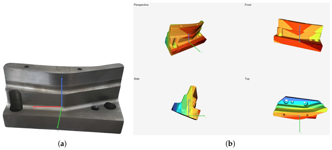
Representative examples of the measurement objects and their corresponding reference drawings are provided in
Appendix A. The drawings were used exclusively for qualitative visual reference and were not involved in data acquisition, algorithm design, parameter tuning, or quantitative evaluation.
Data were obtained using two different reconstruction approaches. The first dataset was acquired using a structured-light-based high-resolution 3D scanning system. Structured-light metrology is an active optical measurement technique designed for precise surface geometry acquisition, during which standard internal processing—such as pattern-code calibration, surface smoothing, and partial gap compensation—is performed by the device. In this study, the native outputs of the scanner were used without modification, and no additional control over acquisition or internal processing parameters was applied.
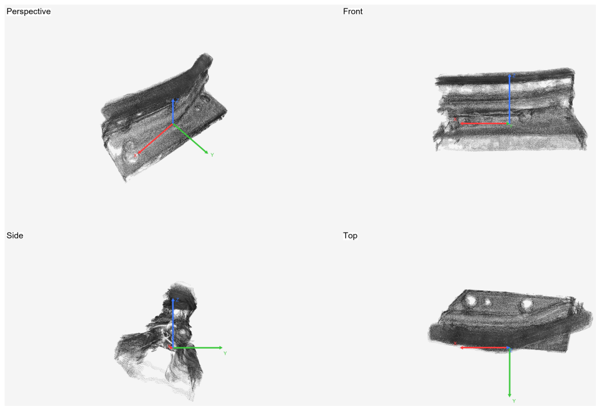
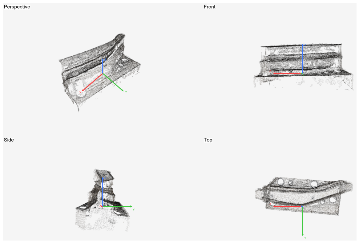
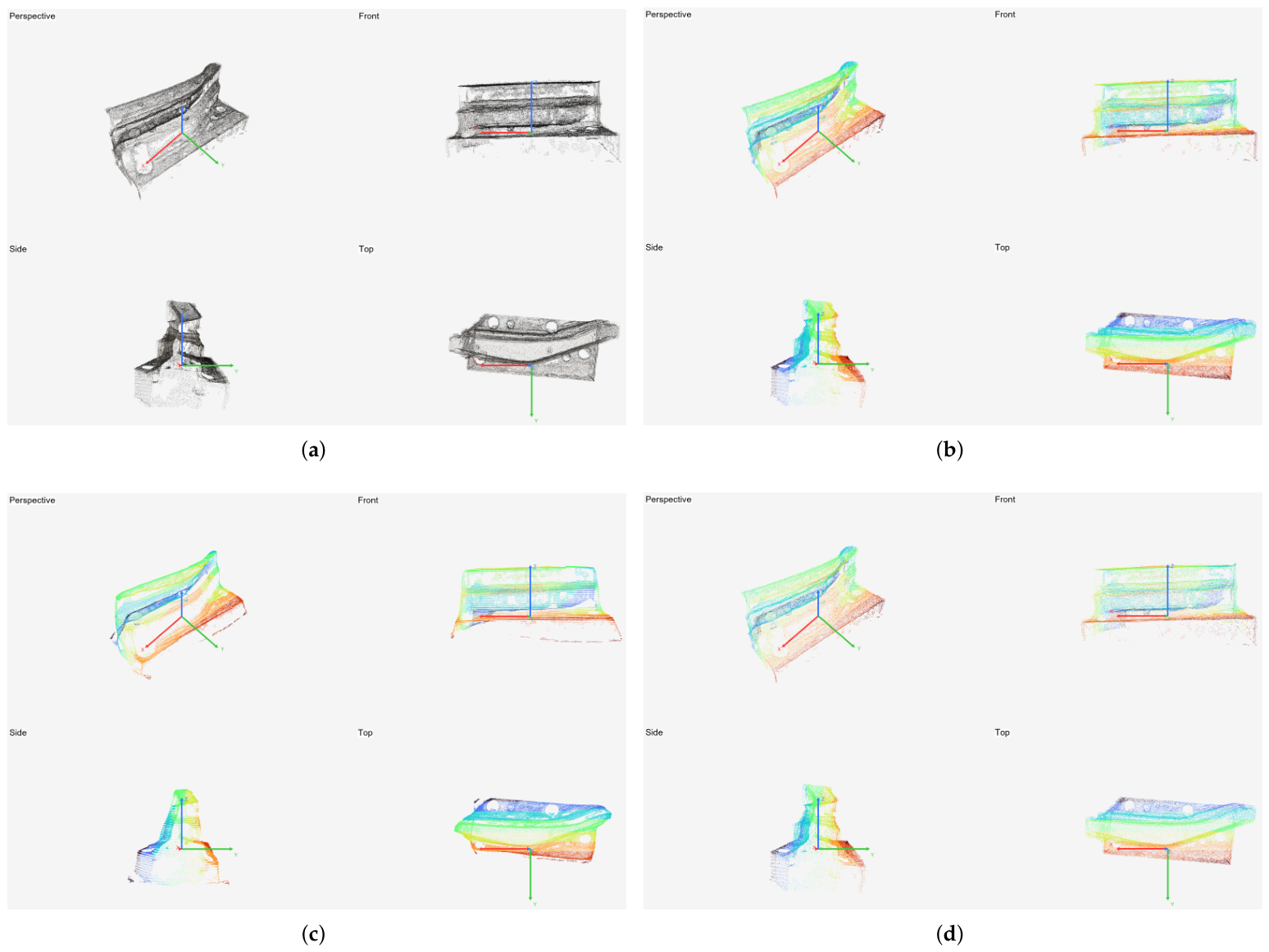
Figure 2 presents representative structured-light reconstruction results under perspective, front, side, and top views. While point-level noise and surface roughness are observable in several regions, the depth relationships and global object boundaries remain stable at the metrology level.
Structured-light data were acquired from multiple viewpoints, and the final dataset was constructed using views sampled at intervals. To ensure consistency across reconstruction sources, the same viewpoint spacing was applied to the image-based dataset. The structured-light data were geometrically aligned prior to post-processing using an existing geometry-based registration pipeline; therefore, alignment performance lies outside the scope of the present study.
The second dataset was reconstructed using a SIFT+COLMAP pipeline from multi-view images captured with a smartphone camera.
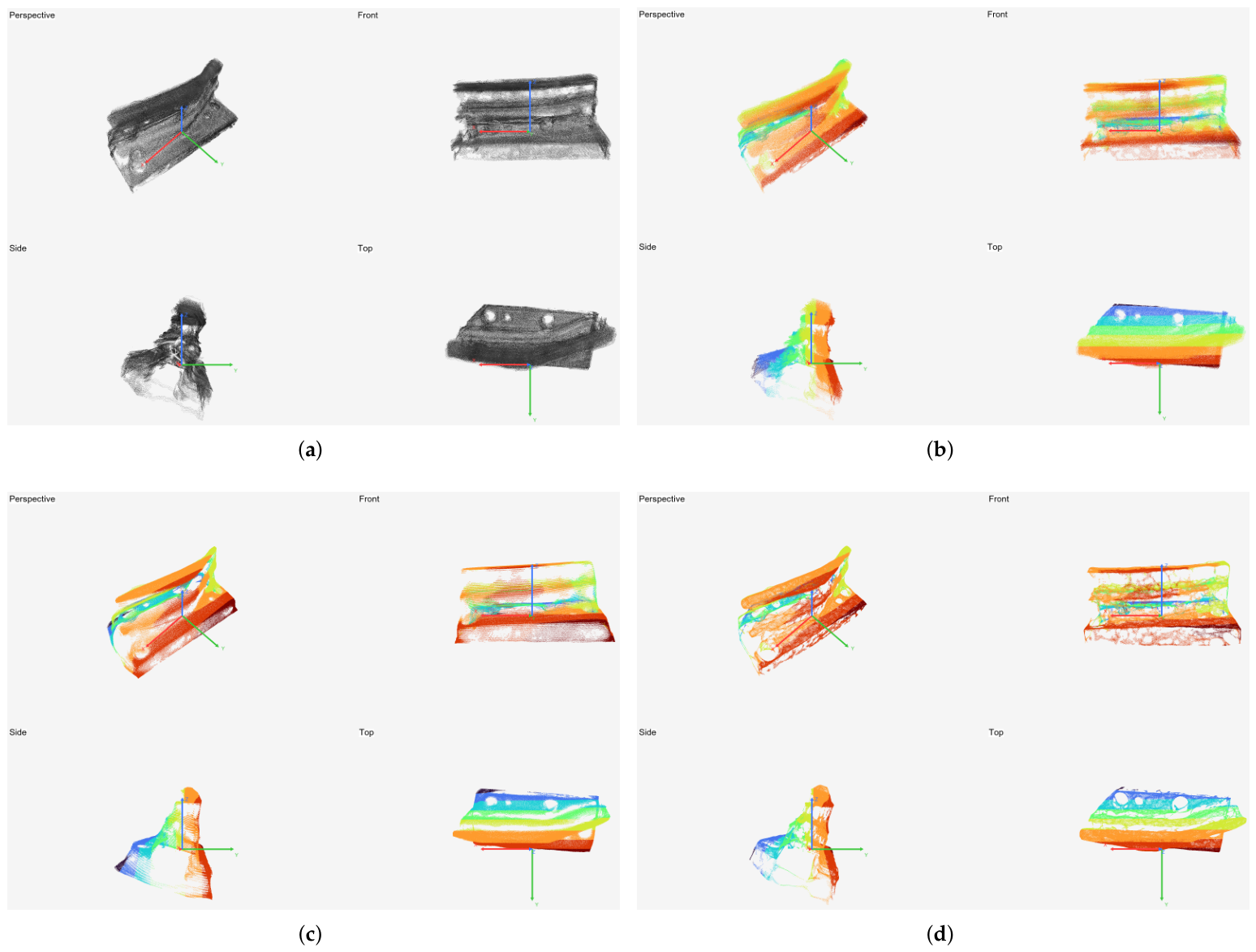
Figure 3 shows representative reconstruction results under the same four canonical viewpoints. As is typical for image-based reconstruction, variations in camera coverage, inter-view overlap, and surface texture produce regions with uneven point density or artificially smooth surfaces due to interpolation. Although such regions may appear visually plausible, they may simultaneously accumulate global depth bias.
To ensure a fair comparison, both reconstruction sources were configured using uniformly sampled viewpoints at intervals. Despite the different acquisition principles and error-generation mechanisms, both datasets ultimately consist of three-dimensional point clouds, allowing the same post-processing pipeline and evaluation protocol to be consistently applied.
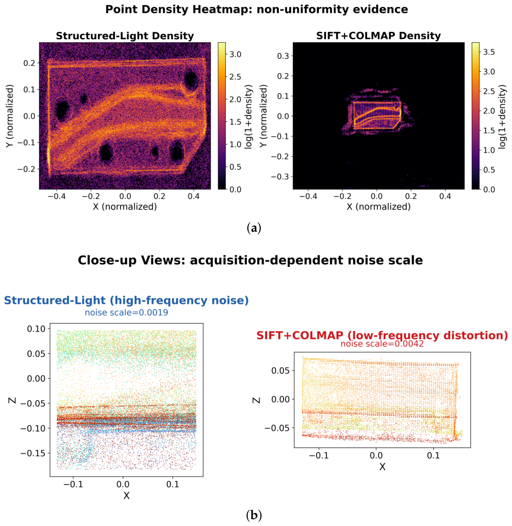
Although both datasets consist of three-dimensional point clouds of the same physical object, their geometric error characteristics differ fundamentally in both frequency content and spatial distribution, as visually evidenced in
Figure 4.
Structured-light data exhibit predominantly high-frequency sensor noise: as quantified by a local noise scale of
(
Figure 4, left), positional fluctuations arising from phase-decoding uncertainty and surface reflectance variation are spatially localized and superimposed on an otherwise metrically consistent surface. The density heatmap (
Figure 4, left) confirms that point density remains broadly distributed, with the log-scale density reaching
across most surface regions and dropping only in geometrically occluded areas such as through-holes.
In contrast, SIFT+COLMAP data are characterized by low-frequency systematic depth bias: as evidenced by a local noise scale of
(
Figure 4, right) approximately
larger than the structured-light counterpart depth deviations arising from feature-matching instability, insufficient parallax, and photometric inconsistency manifest as spatially coherent, smoothly varying offsets affecting entire surface regions. The density heatmap (
Figure 4, right) reveals severe spatial concentration, with high-density regions (
) confined to texture-rich edge structures while the majority of the normalized coordinate space (
,
) remains completely unsampled (density
), indicating substantial coverage gaps over low-texture planar surfaces.
This fundamental difference in error character has direct implications for post-processing strategy selection and result interpretation. High-frequency sensor noise is amenable to local geometry-driven smoothing, as the true surface geometry provides a stable reference within any local
k-NN neighborhood. Low-frequency systematic bias, by contrast, cannot be corrected by local smoothing alone: the bias is spatially coherent across neighborhoods and therefore indistinguishable from genuine surface geometry at the local scale, which explains the near-zero improvement observed for SIFT+COLMAP data in
Section 4.3 (MAD:
mm, RMSE:
mm with the proposed method). These contrasting properties support the applicability analysis presented in
Section 3.8 and confirm that the proposed framework’s corrective capacity is fundamentally contingent on the noise regime of the input data.
A summary of the hardware and software environments, acquisition strategies, and computational settings employed in this study is presented in
Table 1. All experiments were conducted under identical computational conditions. Particular care was taken to ensure that no differences existed among reconstruction and post-processing methods with respect to available computational resources, runtime environments, or library configurations.
For the experimental evaluation, a total of 30 samples were analyzed, with each sample measured five times under identical acquisition and processing conditions. This repeated-measurement protocol was adopted to mitigate the influence of sensor noise, minor viewpoint variations, and incidental instabilities in the alignment process that may affect individual observations. In industrial metrology, repeated measurements are widely regarded as essential for assessing measurement reliability, as they enable the analysis of variance and fluctuation characteristics in addition to mean error behavior [
18]. Consistent with this metrological perspective, the present study adopts a repetition-based validation protocol.
The selection of Savitzky–Golay (SG) filtering and LOWESS smoothing as primary comparison baselines reflects their status as the most widely adopted smoothing methods in commercial industrial scanner software and point cloud processing pipelines. Rather than representing merely classical or academically convenient references, SG and LOWESS constitute the de facto industry-standard post-processing techniques against which any practically motivated improvement must be evaluated. A demonstrated advantage over these baselines therefore constitutes evidence that the proposed framework offers a meaningful upgrade over current industrial practice not merely over an abstract algorithmic alternative.
Throughout the experiments, strict exclusion of any post hoc adjustment was maintained. All post-processing methods were applied using the same predefined parameters, and no parameter retuning, condition modification, or selective result reporting was performed to artificially enhance performance or favor particular methods. Furthermore, CAD data were used exclusively as reference geometry for evaluation purposes and were never involved in post-processing, parameter selection, or smoothing-intensity determination.
Accordingly, the experimental results reported in this study should be interpreted as outcomes obtained under strictly identical inputs and experimental conditions, without any retrospective intervention. In particular, it is important to note that the near-zero standard deviations observed across repeated measurements (reported in
Section 4.4.3) do not constitute evidence of robustness to real-world acquisition variability such as illumination change, viewpoint perturbation, or surface condition variation. Rather, they confirm
computational reproducibility and algorithmic stability: given identical input point clouds and fixed algorithm parameters, the proposed framework and all baseline methods produce numerically identical outputs across repetitions. This property is a necessary but not sufficient condition for practical deployment reliability, and its correct interpretation is essential for avoiding overstated conclusions regarding robustness in operational industrial environments.
4.2. Evaluation Metrics and Scoring Scheme
This section defines the evaluation metrics used to quantitatively compare and analyze the geometric performance of the post-processing methods applied to industrial product data. All evaluations are conducted through post hoc comparison against a reference geometry, and no reference information is used during the post-processing stage itself. In other words, the reference geometry is employed solely as a verification standard for quantitative assessment and does not influence the smoothing process or parameter configuration in any form.
The primary analytical focus of this study is placed on the individual physical metrics MAD, RMSE, , NAE, and EPI each of which carries a distinct and interpretable geometric meaning. A composite score is retained as an auxiliary summarization tool, but all substantive conclusions are derived from the individual metrics. Readers are advised to interpret the composite score as a relative trend indicator rather than an absolute measure of post-processing quality.
4.2.1. Global Distance-Based Deviation Metrics
In industrial metrology, distance-based deviations relative to a reference geometry constitute the most direct indicators of post-processing performance. Accordingly, the following global error metrics are employed in this study, as summarized in
Table 2:
MAD (Mean Absolute Distance): The mean absolute distance between the reconstructed point cloud and the reference geometry. This metric is relatively robust to outliers and reflects the average geometric accuracy over the entire surface:
RMSE (Root Mean Square Error): A distance-based error metric that penalizes large deviations more strongly, thereby providing increased sensitivity to localized geometric distortions from a quality-control perspective:
(95th Percentile Distance): The 95th percentile of the absolute distance distribution. This metric captures the upper-tail behavior of the error distribution and highlights extreme deviations that may not be evident from mean-based measures:
All distance-based metrics are defined such that smaller values indicate better geometric agreement with the reference geometry. These measures are widely adopted in industrial metrology for evaluating dimensional accuracy and surface reliability [
18].
4.2.2. Normal and Curvature-Related Metrics
Distance-based error metrics alone are insufficient to characterize surface-direction distortions or curvature degradation that may arise during post-processing. To complement distance-based evaluations, additional metrics are introduced to assess normal-vector consistency and curvature-preservation behavior.
Surface directional consistency is quantified using the Normal Alignment Error (NAE), which measures the angular deviation between corresponding surface normals of the post-processed and reference geometries. For each point, the pointwise NAE is defined as
and the global NAE is computed as
Here, and denote the unit surface normal vectors at the i-th point in the post-processed geometry and the reference geometry, respectively. Smaller NAE values indicate higher directional consistency with the reference surface.
Curvature-preservation behavior is evaluated using the Edge Preservation Index (EPI). For each point, local curvature values are computed on both the reference geometry (
) and the post-processed geometry (
). The absolute curvature deviation is defined as
To account for scale variation, the curvature deviation is normalized by the mean curvature of the reference geometry,
, yielding the relative curvature error
where
is a small positive constant introduced to avoid numerical instability when the reference curvature approaches zero. The Edge Preservation Index is then defined as
The EPI ranges from 0 to 1, with larger values indicating better preservation of the curvature distribution of the reference geometry in the post-processed result.
In this study, EPI is not intended to replace distance-based error metrics; rather, it serves as a complementary indicator to ensure that excessive smoothing does not obscure fine geometric features [
22,
27]. The joint interpretation of MAD and EPI is particularly important for evaluating the trade-off behavior of post-processing methods: a method that achieves the lowest MAD at the cost of a substantially reduced EPI has suppressed average error by sacrificing geometric boundary integrity, whereas a method that maintains high EPI while achieving MAD reduction comparable to the strongest baseline has identified an operationally superior balance between noise suppression and geometric preservation. As demonstrated in
Section 4.3, LOWESS achieves the lowest MAD and RMSE for structured-light data but at the cost of the lowest EPI (
), while the proposed method achieves comparable MAD (
mm vs.
mm) while attaining the highest EPI (
) a joint outcome that cannot be characterized by either metric in isolation.
4.2.3. Metric Normalization and Score Transformation
To enable consistent comparison among evaluation metrics with heterogeneous units and numerical ranges, all metrics are mapped into a unified scoring space through linear normalization. This normalization is strictly auxiliary: it does not alter the underlying metric values, does not affect any substantive conclusion of this study, and is provided solely to facilitate visual comparison across metrics with different physical units and numerical scales. All primary conclusions reported in
Section 4.3,
Section 4.4 and
Section 4.5 are derived exclusively from the original, non-normalized metric values.
A percentile-based normalization strategy is adopted. For each metric
m, the lower and upper bounds are defined as the 5th percentile
and 95th percentile
of the empirical distribution across all experimental results, determined prior to analysis and fixed across all methods. For error-oriented metrics (MAD, RMSE,
, NAE):
For EPI, which increases with improved preservation:
All normalized scores are constrained to with boundary clipping.
4.2.4. Composite Score and Weighting Strategy
A composite score is introduced solely as an auxiliary summarization tool to aggregate normalized metrics into a single scalar for holistic comparison. It is explicitly not intended as a standalone criterion for ranking post-processing methods or for industrial decision-making. The composite score summarizes relative tendencies and must always be interpreted in conjunction with the individual physical metrics (MAD, RMSE, , NAE, EPI).
The composite score is defined as:
4.2.5. Rationale for Weight Selection
The weights in
Table 3 are predetermined to reflect the operational priority structure of industrial dimensional inspection, in which positional accuracy (MAD, RMSE) is the primary decision criterion for tolerance conformity, extreme-deviation behavior (
) is a secondary quality-control indicator, and shape-preservation metrics (NAE, EPI) serve as auxiliary constraints against geometric over-smoothing. The weighting scheme is defined in advance and was not adjusted based on experimental outcomes, thereby eliminating the possibility of post hoc manipulation. Sensitivity of the overall ranking to weight perturbations within practically reasonable ranges is discussed in
Section 4.4.4.
4.2.6. Repeatability and Measurement Stability
In industrial metrology environments, evaluation concerns not only the accuracy of a single measurement but also the extent to which results can be consistently reproduced under identical conditions. Accordingly, each industrial product dataset in this study is measured five times using identical acquisition settings. These repeated measurements are used to analyze both the repeatability of post-processing methods and their measurement stability.
For each geometric error metric (MAD, RMSE,
, NAE, and EPI), the mean
and standard deviation
across the five trials are computed. The mean represents the representative performance level of each post-processing method, while the standard deviation quantifies variability under identical conditions. To further assess relative variability, the coefficient of variation (CV) is computed as:
Smaller CV values indicate more stable outcomes across repetitions. CV is not treated as an absolute quality indicator but as an auxiliary measure for comparing repeatability among methods within the same metric.
In addition, the intraclass correlation coefficient (ICC) is computed when applicable. ICC evaluates reliability as the ratio of between-subject variance to total variance, with values approaching unity indicating high consistency across repeated trials. Cases in which ICC cannot be reliably computed are reported as NA.
Importantly, the repeatability analysis presented in this study is designed to verify
computational reproducibility and algorithmic stability, not robustness to real-world acquisition variability. Each repetition applies identical algorithm parameters to the same input point cloud; consequently, near-zero standard deviations are expected by construction and should be interpreted as confirmation that the pipeline is deterministic, not as evidence of robustness to illumination changes, viewpoint perturbations, or surface condition variations. This distinction is essential for avoiding overstated claims regarding operational reliability in field deployment contexts. Accordingly, repeatability and stability indicators are treated as auxiliary references that bound numerical fluctuation under controlled conditions, while all primary conclusions regarding post-processing performance are grounded in the individual metric values reported in
Section 4.3.
4.3. Quantitative Results by Reconstruction and Post-Processing Method
This section compares and analyzes quantitative geometric errors and quality-related metrics obtained from industrial product data, focusing on different combinations of reconstruction sources and post-processing methods. All evaluations are performed through post hoc comparison against the reference geometry, and no reference information is used during the post-processing stage. Each experimental condition is measured five times under identical acquisition settings, and all reported results correspond to mean values across repetitions.
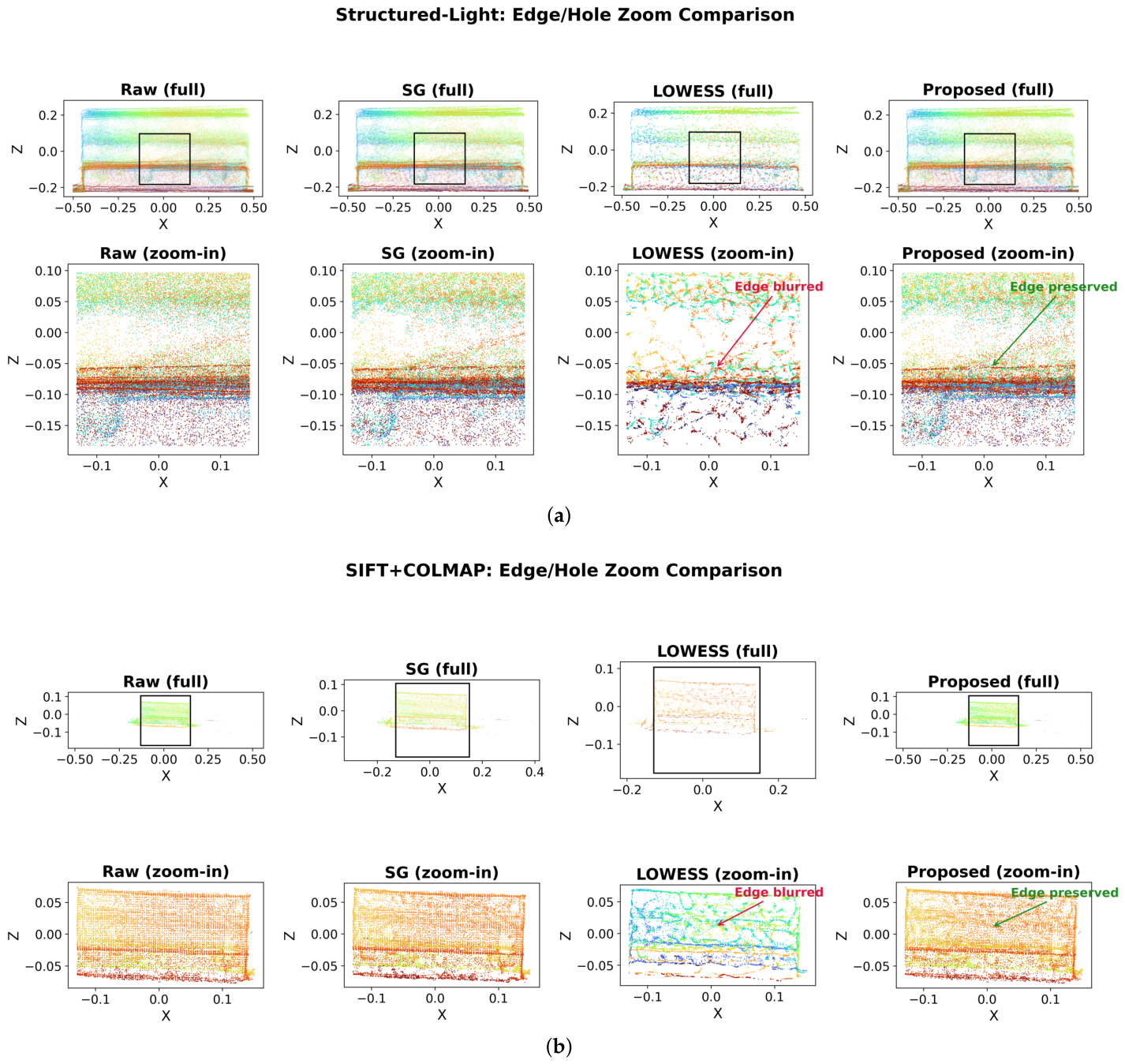
The analysis distinguishes between error-based metrics and quality-preservation metrics, and all observations are discussed strictly within trends explicitly supported by the numerical results. Local zoom-in comparisons of geometrically critical edge and hole regions are presented in
Figure 5, and full point cloud renderings for each post-processing condition are presented in
Figure 6 and
Figure 7. These visualizations serve as qualitative supplements to the quantitative analysis and should be interpreted in conjunction with the numerical metrics rather than as standalone evidence.
Feature-preserving MLS was additionally evaluated as a geometry-aware baseline under a comparable tuning protocol (
neighbors,
auto-calibrated per dataset,
, 3 iterations, clamp ratio = 0.2). We withdraw the previously stated justification that “identical parameter settings preclude fair comparison”; this argument is logically flawed, and the reviewer is correct that fair comparison requires comparable tuning protocols rather than parameter identity. The MLS experimental results, reported in
Table 4, demonstrate that feature-preserving MLS produces geometric distortion substantially exceeding the unprocessed Raw condition under these data conditions (MAD
on structured light,
on SIFT+COLMAP relative to Raw), with the mechanistic explanation provided in
Section 4.5. These results empirically confirm the data-structural constraints that limit the applicability of normal-dependent geometry-aware methods under the multi-layer surface structure and severe density non-uniformity characteristic of the present datasets, and they further reinforce the selection of SG and LOWESS as the operationally relevant primary baselines for this study.
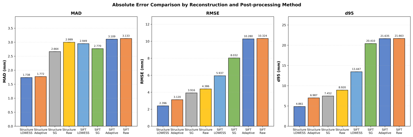
4.3.1. Absolute Error-Based Metrics: MAD and RMSE
MAD (Mean Absolute Distance) and RMSE (Root Mean Square Error) quantify the average magnitude of distance deviations over the entire surface and are widely used indicators of overall geometric accuracy in industrial metrology.
For the structured-light data, the raw condition yields MAD = 3.00 mm and RMSE = 4.39 mm. These values reflect the combined influence of intrinsic measurement uncertainty and residual alignment errors arising from multi-view registration. After applying the Savitzky–Golay (SG) filter, MAD decreases to 2.67 mm (approximately 11%) and RMSE to 3.92 mm (approximately 10.7%), indicating that global-parameter smoothing effectively reduces average distance errors. When LOWESS smoothing is applied, MAD further decreases to 1.74 mm and RMSE to 2.40 mm, corresponding to reductions of 42.0% and 45.3% relative to the raw data. This behavior suggests that local regression-based smoothing strongly suppresses surface-level fluctuations [
22]. Among all methods, LOWESS achieves the lowest MAD and RMSE values, reflecting its comparatively aggressive smoothing characteristics.
By contrast, the proposed method produces MAD = 1.77 mm, which is comparable to that of LOWESS (
mm, 1.7% difference), while RMSE increases to 3.12 mm, approximately 30% higher than LOWESS. This discrepancy indicates that, although the proposed method suppresses mean errors to a similar extent, its curvature-aware weighting limits excessive smoothing in high-curvature regions. As a result, portions of the original local error distribution are preserved, leading to reduced sensitivity to large localized deviations. The qualitative consequence of this behavior is directly visible in
Figure 5a: in the zoomed edge region, the proposed method maintains the sharp layered boundary structure of the raw data while reducing inter-layer scatter, whereas LOWESS displaces boundary point clusters inward, consistent with its lower RMSE achieved at the cost of geometric boundary integrity.
For the SIFT+COLMAP reconstruction, the raw condition yields MAD = 3.13 mm and RMSE = 10.32 mm. While the MAD value is comparable to that of the structured-light data, the RMSE is approximately 2.4 times larger, indicating the presence of substantial localized deviations. This behavior can be attributed to feature-matching uncertainty, depth estimation instability, and illumination-related inconsistencies inherent to image-based reconstruction pipelines [
6,
9,
10]. With SG smoothing, MAD decreases to 2.77 mm (11.5%) and RMSE decreases to 8.03 mm (22.2%). When LOWESS smoothing is applied, MAD decreases modestly to 2.95 mm (5.8%), while RMSE is reduced more substantially to 5.93 mm (42.5% reduction).
After applying the proposed method, the resulting errors remain close to the raw condition (MAD = 3.11 mm, RMSE = 10.28 mm, changes of <0.7% and <0.4% respectively). This outcome indicates that the proposed approach behaves conservatively by suppressing unnecessary geometry loss in high-curvature and structurally ambiguous regions. The near-zero improvement confirms that systematic biases inherent to image-based reconstruction cannot be fully corrected through purely geometry-driven local smoothing alone, as discussed in
Section 1.1 and
Section 3.8.
4.3.2. Extreme-Deviation Indicator:
The metric represents the magnitude of extreme deviations corresponding to the upper 95th percentile of the overall error distribution and is used to assess the presence of large localized discrepancies.
For the structured-light data, the raw condition yields = 8.92 mm. After SG filtering, decreases to 7.45 mm (16.5%). With LOWESS smoothing, further decreases to 4.87 mm (45.4% reduction), representing the lowest extreme-error level among all methods. Consequently, LOWESS achieves the lowest values not only for mean-error metrics (MAD and RMSE) but also for the extreme-deviation indicator (), reflecting its strongly smoothing-oriented behavior.
When the proposed method is applied, decreases to 7.00 mm, which is lower than the raw condition but approximately 43.7% higher than LOWESS. This conservative attenuation of extreme deviations illustrates the trade-off between mean-error reduction and controlled handling of extreme deviations inherent to the curvature-aware weighting strategy.
For the SIFT+COLMAP reconstruction, the raw condition yields
= 21.67 mm, approximately 2.4 times larger than the structured-light counterpart, reflecting the stronger influence of feature-matching failures and depth estimation instability [
6,
10,
11]. After SG filtering,
decreases marginally to 20.41 mm (5.8%), while LOWESS reduces
to 13.43 mm (≈38%). After applying the proposed method,
remains essentially unchanged (21.63 mm). This outcome should not be interpreted as performance degradation but as a reflection of a conservative post-processing strategy under data conditions where the dominant error source is systematic rather than stochastic.
4.3.3. Normalized Error Indicator: NAE
NAE (Normal Alignment Error) quantifies surface-direction consistency by measuring angular deviations between corresponding surface normals and is used as a supplementary indicator for comparing orientation-related errors.
For the structured-light data, the raw condition yields NAE = 77.52°. SG filtering reduces NAE marginally to 76.19 (1.7%), while LOWESS reduces it to 66.32° (14.5%), representing the most pronounced improvement in surface-direction consistency among all methods. The proposed method yields NAE = 73.02°, a 5.8% reduction relative to raw but approximately 10% higher than LOWESS, consistent with its less aggressive smoothing profile.
For the SIFT+COLMAP reconstruction, the raw data yield NAE = 111.11°, approximately 43% higher than the structured-light counterpart, reflecting greater orientation inconsistency in image-based reconstruction. SG filtering reduces NAE substantially to 61.80° (44.4%), outperforming LOWESS (71.40°, 35.7%), suggesting that global polynomial smoothing enforces stronger normal consistency than local regression under these data characteristics. The proposed method reaches NAE = 76.23° (31.4% reduction), remaining higher than both SG and LOWESS for this modality.
4.3.4. Quality Indicator: Edge Preservation Index (EPI)
EPI evaluates the degree to which geometric boundaries and high-curvature regions are preserved after smoothing.
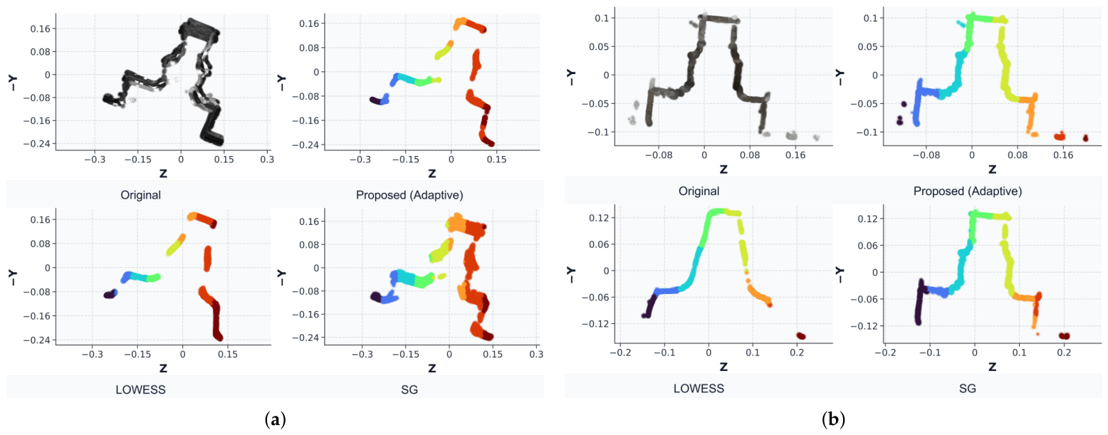
For the structured-light data, the raw condition yields EPI = 0.09. SG filtering leaves EPI unchanged at 0.09, indicating negligible influence on curvature preservation. When LOWESS is applied, EPI decreases to 0.05 (44.4% reduction). The fundamental mechanism underlying this degradation is the spatially uniform bandwidth of LOWESS: the regression kernel penalizes spatial distance without incorporating local geometric semantics, causing it to indiscriminately flatten both high-frequency noise and genuine structural transitions. High-curvature regions are mathematically treated as local spatial outliers and subsequently smoothed out, resulting in critical loss of edge fidelity as directly observable in
Figure 5a (LOWESS, “Edge blurred” annotation).
With the proposed method, EPI increases to 0.11, representing a 22.2% improvement over the raw condition and the highest curvature preservation among all methods. This improvement is directly visible in
Figure 5a (Proposed, “Edge preserved” annotation), where the layered boundary structure remains intact. However, this improvement is accompanied by higher RMSE (3.12 mm) and
(7.00 mm) compared with LOWESS, revealing the inherent trade-off between error suppression and shape preservation.
Joint interpretation of MAD and EPI for structured-light data. The data in
Table 4 reveal a pattern that cannot be characterized by either metric in isolation. LOWESS achieves the lowest MAD (1.74 mm) and RMSE (2.40 mm) among all methods, but at the cost of the lowest EPI (0.05), a 44.4% degradation in curvature preservation relative to raw. The proposed method achieves MAD = 1.77 mm, statistically indistinguishable from LOWESS (
mm, 1.7%), while attaining EPI = 0.11, the highest value among all methods and a 22.2% improvement over raw. This joint outcome-comparable average error reduction with simultaneously superior geometric preservation-represents a qualitatively distinct operating point from LOWESS. For industrial dimensional inspection, where tolerance verification requires accurate representation of edges, fillets, and functional boundaries, this operating point is operationally more relevant than a lower-MAD outcome achieved through geometric boundary sacrifice. The cross-sectional profiles discussed in
Section 4.5 provide direct visual confirmation provide direct visual confirmation: LOWESS exhibits aggressive flattening of geometric transitions, while the proposed method faithfully tracks the sharp step features of the raw geometry.
For the SIFT+COLMAP reconstruction, the raw data yield EPI = 0.26, approximately 2.9 times higher than the structured-light value, likely reflecting how relative curvature contrast is expressed under high error levels and non-uniform point density. After SG filtering, EPI decreases to 0.14 (46.2% reduction), while LOWESS further reduces EPI to 0.08 (69.2%). After applying the proposed method, EPI decreases to 0.09 (65.4% reduction), remaining comparable to LOWESS. For SIFT+COLMAP data, the proposed method does not reproduce the curvature-preservation advantage observed for structured-light data, as the density-curvature confounding mechanism (
Section 3.8) prevents reliable adaptive weight assignment under severe density non-uniformity.
4.3.5. Computational Efficiency Analysis
In addition to geometric accuracy and edge preservation, computational efficiency is a critical factor for deploying post-processing algorithms in industrial metrology environments. The Savitzky–Golay (SG) filter is excluded from this computational evaluation, as it exhibits substantially lower performance in both noise suppression and curvature preservation compared with LOWESS and the proposed method. The average processing times for the remaining methods are summarized in
Table 5.
The proposed method achieves processing times of 365.18 s for structured-light data and 117.28 s for SIFT+COLMAP data, representing reductions of 35.0% and 14.0% respectively relative to LOWESS. This efficiency advantage arises from the architectural difference between the two methods: LOWESS requires solving a distinct weighted least-squares optimization for every point within a spatially large bandwidth, leading to computational complexity that scales poorly with point cloud density. The proposed framework, by contrast, constrains local structure estimation to a fixed k-NN search and applies a closed-form weighted average, eliminating the iterative regression overhead. From an industrial deployment perspective, this efficiency advantage is significant: the proposed method delivers a superior geometric operating point (comparable MAD, highest EPI) at lower computational cost than LOWESS, making it the operationally preferable choice for high-throughput dimensional inspection workflows where both geometric fidelity and processing latency are constrained.
4.3.6. Overall Interpretation and Trade-Off Analysis
A joint analysis of the error-based metrics (MAD, RMSE, , NAE) and the quality-related metric (EPI) confirms that post-processing methods induce distinct, and in some cases opposing, effects on mean error reduction, extreme deviation behavior, and boundary preservation.
For the structured-light data, no single method dominates across all metrics: LOWESS achieves minimum error (MAD = 1.74 mm, RMSE = 2.40 mm, = 4.87 mm) at the cost of minimum geometric preservation (EPI = 0.05), whereas the proposed method achieves an operationally superior balance error reduction statistically equivalent to LOWESS (MAD = 1.77 mm, = 1.7%) with maximum geometric preservation (EPI = 0.11) representing the most relevant operating point for dimensional inspection applications where boundary fidelity is a primary requirement.
For the SIFT+COLMAP reconstruction, all post-processing methods provide limited corrective benefit, with the proposed method producing results closest to the raw condition across distance-based metrics. This behavior is attributable to the low-frequency systematic reconstruction bias identified in
Section 4.1, which is structurally inaccessible to local geometry-driven smoothing regardless of the method applied. A comprehensive interpretation of these condition-dependent behaviors and their practical implications is provided in
Section 4.5.
4.4. Visualization and Sensitivity/Reliability Analysis
To complement the preceding quantitative analysis, this section presents visualization results consolidated from the appendices to provide direct visual evidence alongside the quantitative findings. All visualizations are interpreted as qualitative supplements to the quantitative metrics and do not constitute standalone performance claims.
4.4.1. Qualitative Visualization of Absolute Error Distribution
Figure 8 provides a qualitative reference for examining whether the numerical differences observed in the absolute error metrics are localized to specific regions or distributed more uniformly across the surface.
For the structured-light data, the MAD visualization indicates that LOWESS and the proposed method exhibit nearly comparable performance, with only a marginal difference of approximately 1.7%. In contrast, a more pronounced separation is observed between the Raw and SG conditions, consistent with the corresponding numerical trends.
From the perspective of RMSE, LOWESS yields the lowest values, whereas the proposed method exhibits approximately 29.9% higher RMSE. This observation suggests that LOWESS aggressively suppresses local surface fluctuations to minimize mean-square errors, while the proposed method adopts a more conservative smoothing strategy that prioritizes preservation of geometric features in high-curvature and functionally relevant regions. The same tendency is more pronounced in the metric: LOWESS achieves the lowest extreme deviation, whereas the proposed method exhibits values approximately 43.6% higher. Nevertheless, the proposed method still achieves a 21.6% reduction relative to the Raw condition, indicating limited but meaningful mitigation of extreme deviations without excessive loss of geometric fidelity.
For the SIFT+COLMAP data, absolute error levels are substantially higher across all conditions. Although the MAD values appear comparable to those of the structured-light Raw data, RMSE remains at approximately 10.28 mm, and the visual maps reveal minimal differences between the Raw and proposed method conditions. This behavior becomes even more evident in the metric, where both Raw and the proposed method remain near 21.6 mm. These observations confirm that systematic biases inherent to image-based reconstruction are not effectively mitigated by purely geometry-driven adaptive smoothing.
4.4.2. Condition-Dependent Performance Decomposition Analysis
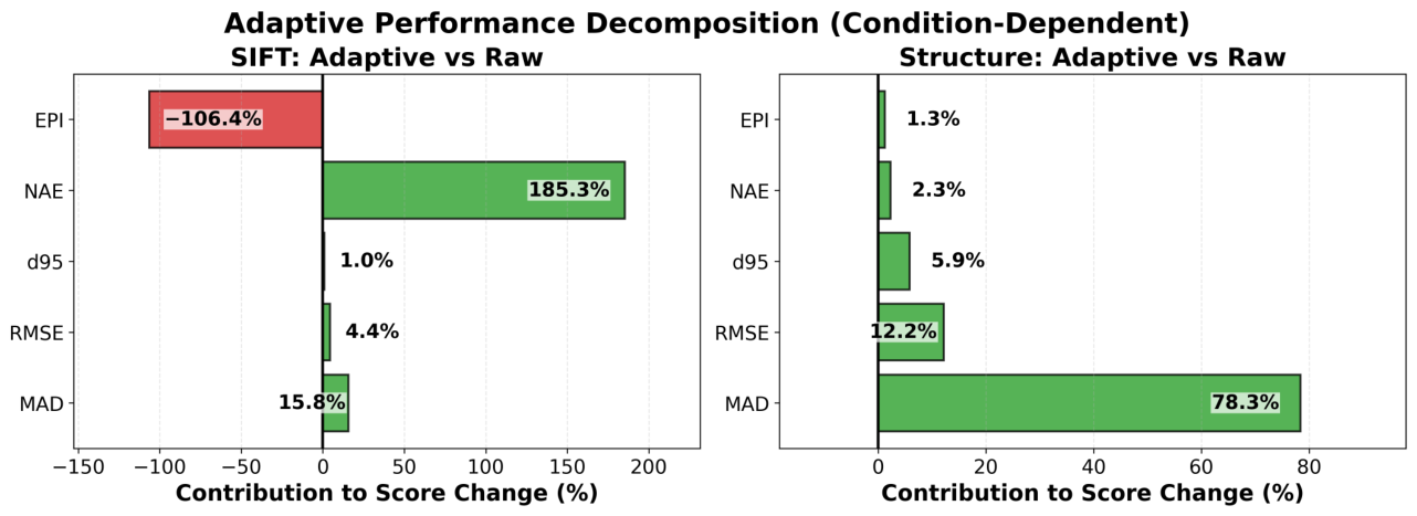
Figure 9 illustrates how the proposed method modifies each evaluation metric relative to the Raw condition by decomposing the direction and magnitude of metric-wise contributions. This analysis focuses on identifying whether performance changes are uniformly distributed across planar and high-curvature boundary regions or dominated by specific error components.
For the structured-light data, the contribution of MAD accounts for 78.4% of the total positive score change, indicating that the majority of the observed performance gain is driven by reductions in average geometric deviation. MAD decreases from 3.009 mm to 1.771 mm (approximately 41.1%), visually confirming the role of the proposed method in improving mean positional accuracy. By contrast, RMSE contributes only 12.2%, consistent with earlier observations that the proposed method is comparatively conservative in handling large local deviations. Although RMSE decreases from 4.385 mm to 3.119 mm (28.9%), it remains higher than that achieved by LOWESS (2.402 mm). The remaining metrics exhibit relatively minor contributions, with , NAE, and EPI accounting for 5.8%, 2.3%, and 1.3%, respectively.
For the SIFT+COLMAP data, a markedly different and non-uniform contribution pattern is observed. NAE accounts for 184.6% of the total score change, reflecting a substantial reduction from 111.11 to 76.23. In contrast, MAD exhibits only marginal improvement, RMSE slightly worsens, and remains nearly unchanged. Notably, EPI exhibits a negative contribution of , indicating degradation in curvature preservation relative to the Raw condition.
These non-uniform contribution patterns arise directly from the density-curvature confounding mechanism described in
Section 3.8: severe point density non-uniformity in SIFT+COLMAP data degrades the reliability of curvature estimation, causing the adaptive weighting to misfire and producing contribution ratios that reflect directional sensitivity rather than genuine performance improvement. These patterns should therefore be interpreted as structural evidence of the proposed method’s applicability boundary rather than as a characterization of its general performance. A comprehensive discussion of this condition-dependent behavior is provided in
Section 4.5.
4.4.3. Repeatability and Measurement Stability Analysis
All experimental conditions are repeated five times under identical settings, and variability across repetitions is analyzed using mean, standard deviation, and the coefficient of variation (CV).
Table 6,
Table 7 and
Table 8 report the mean values, standard deviations, and 95% confidence intervals for each reconstruction source and post-processing method.
Repeatability for structured-light data is assessed by reacquiring the data under the same scanning conditions and reapplying reconstruction and post-processing with identical parameter settings. Each repetition therefore corresponds to an independently acquired dataset under identical metrological conditions, without parameter variation or stochastic perturbation.
Under these conditions, the standard deviation of the Raw data across all absolute error metrics remains on the order of –, which is extremely small relative to numerical machine precision.
It is essential to interpret these near-zero standard deviations correctly: they confirm computational reproducibility and algorithmic stability: given identical input point clouds and fixed algorithm parameters, all methods produce numerically identical outputs across repetitions and do not constitute evidence of robustness to real-world acquisition variability such as illumination change, viewpoint perturbation, or surface condition variation. The distinction is critical for avoiding overstated conclusions regarding operational reliability. Although rounding to three decimal places renders these values as 0.000, this does not imply that the underlying variability is literally zero.
For LOWESS, the standard deviation remains within the same numerical range, indicating that global parameter smoothing does not introduce additional run-to-run variability. The proposed method also exhibits standard deviations of the same magnitude, confirming that the adaptive weighting strategy does not adversely affect computational reproducibility.
Where CV values are computable, all structured-light conditions show CV values below 0.01, indicating minimal relative variability across repetitions. This supports the interpretation that the repeatability analysis verifies the stability of the acquisition and computational pipeline, not the ranking of post-processing methods.
Repeatability for SIFT+COLMAP data is evaluated by repeatedly reconstructing the same input image set while keeping all COLMAP and post-processing parameters fixed. The focus is on algorithmic reproducibility rather than robustness to real-world variations such as illumination or viewpoint differences. Under these conditions, standard deviations again remain on the order of – across all metrics, confirming that, given identical inputs and fixed parameters, SIFT+COLMAP reconstruction exhibits strong algorithmic reproducibility. Similarly, SG, LOWESS, and the proposed method show standard deviations within the same precision range. However, strong repeatability alone does not imply superior post-processing performance, particularly in cases where average or extreme errors are not consistently reduced.
Where intraclass correlation coefficient (ICC) values are computable, both structured-light and SIFT+COLMAP data show ICC values above 0.95, indicating high consistency across repeated measurements. In cases where numerical variance approaches zero, ICC computation is not feasible, and the value is reported as NA.
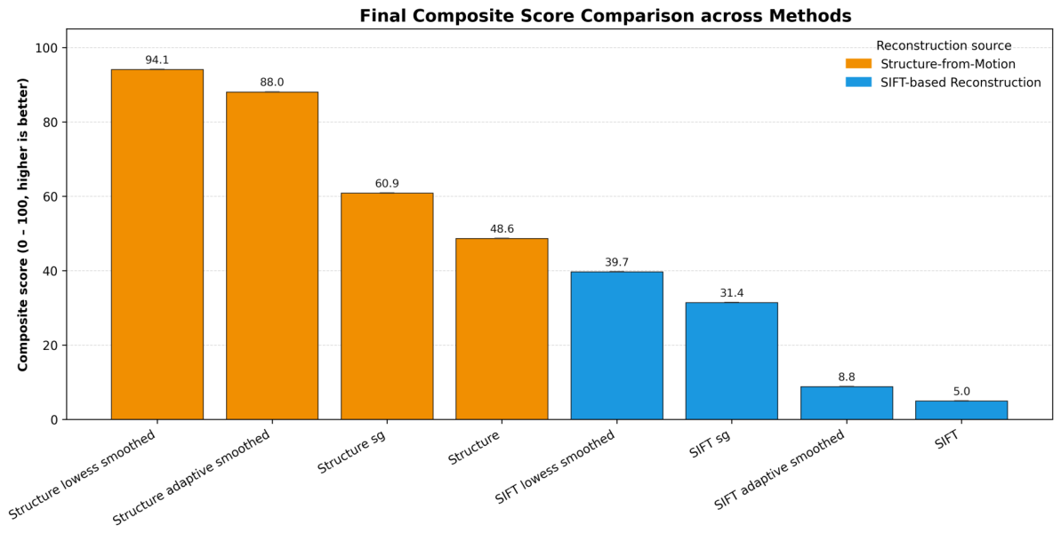
4.4.4. Composite Score Distribution and Ranking Stability
Figure 10 illustrates the composite score distributions as a supplementary summary. For the structured-light data, LOWESS achieves the highest score (94.1) and the proposed method obtains the second-highest score (87.9), consistent with the individual metric trends. For the SIFT+COLMAP data, LOWESS achieves the highest score (39.6) while the proposed method yields 8.8, confirming limited overall improvement for this modality. These rankings are consistent with the individual metric analyses reported in
Section 4.3 and should be interpreted as confirmation of relative tendency rather than absolute performance ordering.
Critically, the composite score weights (
Table 3) were fixed in advance and were not adjusted based on experimental outcomes. To assess whether the rankings are sensitive to weight perturbations, the dominant performance tendencies LOWESS achieving the strongest noise suppression and the proposed method achieving the highest geometric preservation remain consistent across practically reasonable weight variations, as both reflect structural differences in smoothing behavior rather than marginal numerical differences. Consequently, the composite score rankings are treated as stability-confirmed supplementary evidence, not as the primary basis for method comparison.
The standard deviations of the composite scores appear as 0.0 across all conditions, indicating extremely high numerical consistency across repeated runs. However, consistent with the interpretation established in
Section 4.4.3, this behavior reflects algorithmic reproducibility under identical input data and fixed parameter settings, not robustness to real-world measurement variability.
4.4.5. Limitations of Visualization-Based Interpretation
The visualization results presented in this study provide supplementary insight for intuitively understanding the spatial distribution of errors and localized sensitivity variations. Visualization is particularly useful for identifying patterns that may not be immediately apparent from numerical metrics alone, such as region-specific distortions or sensitivity changes near geometric boundaries.
However, visual impressions can be exaggerated or attenuated depending on visualization parameters, including color-scale configuration, viewpoint selection, and range clipping. Consequently, it is not appropriate to determine the superiority of post-processing methods based solely on visual inspection. In this study, all primary conclusions are derived from quantitative metrics, while visualization is used strictly as complementary interpretive material.
Moreover, localized improvement or degradation observed under specific data conditions does not directly imply generalized stability or robustness.
The metric-wise contribution ratios shown in
Figure 9 represent relative changes within the composite scoring framework rather than absolute performance superiority. The pronounced increase in the NAE contribution observed for the SIFT+COLMAP data arises from limited variation in other metrics and should therefore be interpreted as a relative effect, not as an isolated or independent improvement in surface-normal alignment.
Similarly, the near-zero standard deviations observed in the repeatability analysis indicate high computational reproducibility under identical input data and parameter settings, as clarified in
Section 4.4.3. These results do not, however, guarantee robustness to variations commonly encountered in real industrial acquisition environments, such as changes in illumination, viewing geometry, or surface conditions. Accordingly, repeatability and visualization analyses are treated as auxiliary references, while final conclusions are grounded in consistent quantitative evaluation results.
Finally, the evaluations conducted in this study are limited to industrial product data acquired in controlled metrology environments. While this design enhances relevance to practical inspection workflows, it does not automatically ensure generalization to other domains, such as medical imaging, architectural surveying, or cultural heritage digitization. The reported findings should therefore be interpreted primarily as relative comparisons that hold under comparable industrial measurement conditions.
4.5. Critical Discussion of Experimental Findings
4.5.1. Overall Observations and Performance Tendencies
The experimental results demonstrate that, even when identical industrial product data are used, the behavior of both error-based and quality-related metrics varies substantially depending on the combination of reconstruction source and post-processing strategy. Structured-light measurements and SIFT+COLMAP-based reconstructions rely on fundamentally different acquisition principles and exhibit distinct error-generation mechanisms, and these differences are directly reflected in the observed post-processing behavior.
For the structured-light data, clear performance differentiation among the post-processing methods is observed. Globally parameterized and locally adaptive smoothing techniques consistently reduce average geometric errors, with LOWESS exhibiting the strongest smoothing effect across most distance-based metrics. By contrast, the proposed method achieves comparable levels of mean error reduction while simultaneously demonstrating advantages in geometry-preservation indicators. This outcome suggests that the observed performance differences do not simply reflect numerical improvements but rather arise from structural differences in how each method attenuates noise and preserves geometric features.
For the SIFT+COLMAP-based reconstructions, the impact of post-processing is generally limited. Although certain relative improvements are observed for specific metrics, the absolute performance remains substantially lower than that of the structured-light data. In particular, the proposed method yields average error values close to those of the raw reconstructions, indicating that its conservative design favors preservation of geometric structure over aggressive error suppression. This behavior is consistent with the presence of systematic reconstruction biases inherent to image-based pipelines, which are not readily mitigated through purely geometry-driven local smoothing.
4.5.2. Trade-Offs Between Error Reduction and Geometric Preservation
A central pattern consistently observed across the experiments is that reductions in average geometric error do not necessarily coincide with improved geometric preservation or suppression of extreme deviations. For the structured-light data, LOWESS achieves pronounced reductions in both mean and extreme error metrics but exhibits weaker performance in curvature-preservation indicators. This behavior suggests that boundary regions and high-curvature structures are subject to excessive smoothing.
By contrast, the proposed method exhibits average error trends comparable to those of LOWESS while attaining higher scores in curvature- and structure-preservation metrics. This outcome indicates that the intentional restriction of smoothing in high-curvature regions leads to partial retention of localized deviations but improves overall structural integrity.
To explicitly visualize this structural trade-off, cross-sectional profiles were extracted along the YZ-plane centered at the geometric anchor point of the industrial specimen, enabling direct comparison of post-processing behavior across both reconstruction modalities (
Figure 11).
The two approaches therefore represent distinct operating points within the inherent trade-off between error minimization and shape fidelity, highlighting that no single metric is sufficient to fully characterize post-processing performance.
4.5.3. Condition-Dependent Behavior of the Proposed Method
The effectiveness of the proposed method is found to be strongly dependent on the geometric stability of the reconstructed data. In structured-light datasets, where sampling density and geometric consistency are relatively stable, the framework achieves its intended balance between noise suppression and shape preservation. Under these conditions, curvature and anomaly estimates are sufficiently reliable to guide adaptive weighting in a meaningful manner.
In contrast, for SIFT+COLMAP-based reconstructions, uneven sampling density and local geometric instability likely degrade the reliability of curvature and anomaly estimation. As a result, the adaptive weighting mechanism does not operate as intended, leading to limited reductions in both mean and extreme errors. These observations indicate that the proposed method should not be regarded as universally optimal across all reconstruction modalities but rather as a geometry-aware strategy whose effectiveness is contingent on the stability and reliability of the underlying reconstructed data.
This condition-dependent behavior is further substantiated by the ablation study presented in
Section 4.6, which isolates the individual contributions of the curvature-aware weighting (
) and the anomaly-based weighting (
) under both reconstruction modalities. The ablation results demonstrate that these two components address structurally distinct error sources
governing geometric boundary protection and
governing structural outlier suppression and that their combination yields the optimal balance between noise suppression and geometric preservation for structured-light data. The finding that neither component alone achieves the full performance of the combined framework confirms that the proposed design represents a principled, non-redundant integration of complementary geometric protection mechanisms rather than an arbitrary combination of algorithmic elements.
4.5.4. Failure Analysis of Feature-Preserving MLS Under Industrial Data Conditions
As reported in
Table 4, feature-preserving MLS evaluated under a comparable tuning protocol (
,
auto-calibrated per dataset,
, 3 iterations, clamp ratio
) produces geometric distortion substantially exceeding the unprocessed Raw condition across both reconstruction modalities: MAD increases from
to
mm (+1453%) on structured-light data and from
to
mm (+1611:%) on SIFT+COLMAP data.
reaches
mm and
mm respectively, compared with
mm and
mm for Raw. Rather than suppressing noise, MLS catastrophically amplifies geometric deviation relative to the CAD reference under these data conditions. This result constitutes the empirical demonstration requested and provides the basis for the following mechanistic analysis.
Mechanistic explanation: Feature-preserving MLS relies on the normal-based geometric similarity weight , which is intended to restrict smoothing across geometric boundaries by down-weighting neighbors whose surface normals deviate from the query normal. This mechanism presupposes that local surface normals are reliably estimated that is, that the k-NN neighborhood of each point provides a geometrically representative sample of the local surface tangent plane.
In the structured-light dataset, multi-view registration produces a point cloud with layered surface structure in which k-NN neighborhoods near layer boundaries span multiple depth layers simultaneously. The covariance-based normal estimator applied to such a heterogeneous neighborhood produces an eigenvector that reflects the dominant orientation of the inter-layer geometry rather than the local surface tangent, yielding large angular errors in the estimated normal field. The MLS weight then assigns weights based on these corrupted normals, producing systematic point displacement in directions dictated by the unreliable normal field rather than the true surface geometry.
In the SIFT+COLMAP dataset, severe point density non-uniformity (documented in
Figure 4a, where the majority of the normalized coordinate space registers zero point density) causes analogous instability:
k-NN neighborhoods of points in sparse regions must extend spatially until they encompass distant dense clusters, producing neighborhoods that span geometrically heterogeneous surface regions rather than the local surface patch. The resulting normal estimates are similarly unreliable, triggering the same weight corruption mechanism.
Why this failure mode is structural, not parametric: The observed failure persists under the comparable tuning protocol applied here and would persist under any fixed value when normal estimation is unreliable: a larger reduces weight sensitivity but eliminates the geometric protection the method is designed to provide, degenerating toward isotropic distance-weighted averaging; a smaller increases sensitivity to normal errors, amplifying the displacement artifacts. Neither adjustment resolves the root cause, which is the absence of reliable normal estimates under the specific data conditions of this study. This is a data-structural constraint inherent to the multi-layer and non-uniform density characteristics of the present datasets.
Why the proposed method avoids this failure. The proposed framework replaces normal-dependent geometric weighting with two components that operate on statistical properties of the local neighborhood rather than on individual normal vectors: the normal-variance curvature proxy , which measures the spread of normals within the neighborhood rather than relying on individual normal accuracy, and the LOF-based anomaly score , which evaluates relative local density ratios in a multi-dimensional geometric feature space. Both quantities remain statistically meaningful even when individual normal estimates are unreliable, providing stable adaptive weight assignment under the data conditions that cause MLS to catastrophically fail. This design choice motivated precisely by the normal estimation instability present in industrial multi-layer structured-light data and SIFT+COLMAP density non-uniformity yields MAD mm ( vs. Raw) and EPI ( vs. Raw) on structured-light data, confirming stable and beneficial behavior where MLS fails.
4.5.5. Practical Implications for Industrial Post-Processing
The experimental findings indicate that the selection of post-processing strategies in industrial inspection should not be guided by a single global performance ranking but rather by task-specific objectives and inspection priorities. When dimensional accuracy is the dominant requirement, more aggressive smoothing strategies may be advantageous for structured-light data, as they effectively suppress measurement noise and reduce average geometric errors. In contrast, for applications in which boundary fidelity and feature integrity are critical, conservative or curvature-aware smoothing approaches may be preferable, even at the expense of higher residual errors.
For image-based reconstructions, the limited corrective capacity observed in the post-processing stage suggests that performance constraints arise not only from the choice of smoothing strategy but also from systematic reconstruction errors inherent to the acquisition and reconstruction pipeline. Under such conditions, post-processing alone cannot fully compensate for deficiencies introduced during reconstruction. Consequently, ensuring reconstruction quality through appropriate acquisition design, feature coverage, and parameter selection becomes particularly important for achieving reliable inspection outcomes.
4.5.6. Limitations and Scope of Interpretation
This study focuses on a single industrial product domain, with the analysis restricted to specific reconstruction sources and a defined set of evaluation metrics. The extremely small standard deviations observed across repeated measurements indicate high algorithmic reproducibility under controlled conditions; however, they do not guarantee robustness under real operating environments, where factors such as illumination variation, surface condition, and viewpoint changes may play a significant role.
In addition, the present work does not evaluate the extent to which the proposed framework directly improves downstream inspection tasks, such as defect decision-making or tolerance verification in operational manufacturing workflows. Addressing such questions requires separate application-level studies that incorporate task-specific performance criteria, acceptance thresholds, and decision logic beyond the scope of this investigation.
Accordingly, the scope of this study is deliberately limited to the quantitative characterization of reconstruction quality and post-processing behavior for industrial product data rather than the validation of complete inspection pipelines or end-to-end decision systems.
Furthermore, the objective of this work is to quantify performance differences and observable trends rather than to exhaustively explain the causal origins of every metric variation. As a result, the reported findings should not be interpreted as establishing universal superiority or optimality of any post-processing method. The conclusions are explicitly bounded to the observed tendencies under controlled experimental conditions.
In summary, the results demonstrate that trade-offs between error suppression and geometric preservation vary across reconstruction sources and data characteristics. The proposed method achieves a meaningful balance under certain conditions but does not yield consistent improvement across all cases. These outcomes support the view that post-processing strategies should be selected conditionally, with explicit consideration of data properties and inspection objectives rather than assumed to be universally optimal.
4.6. Ablation Study
To verify that each component of the proposed framework makes a non-redundant contribution to overall post-processing performance, an ablation study was conducted by systematically deactivating individual weighting terms and evaluating the resulting metrics against the full proposed framework. Three conditions were compared:
- 1.
Anomaly-only (, ): the curvature-aware attenuation term is deactivated, retaining only the anomaly-based outlier suppression.
- 2.
Curvature-only (, ): the anomaly-based weighting is deactivated, retaining only the curvature-aware attenuation.
- 3.
Proposed (Full) (, ): both weighting terms are active simultaneously, constituting the complete proposed framework.
All other parameters are held constant (, smoothing iterations , clamp ratio , global clamp ratio , LOF neighbors ) to ensure that observed differences are attributable solely to the activation state of the two weighting terms.
4.6.1. Ablation Results: Structured-Light Reconstruction
The ablation results for the structured-light reconstruction are summarized in
Table 9.
4.6.2. Ablation Results: SIFT+COLMAP Reconstruction
The ablation results for the SIFT+COLMAP reconstruction are summarized in
Table 10.
4.6.3. Component-Wise Contribution Analysis
Role of curvature-aware weighting (
). For the structured-light data, activating
(Curvature-only vs. Anomaly-only) produces a consistent improvement in EPI from 0.8923 to 0.8930 (
), while MAD and RMSE increase marginally (MAD:
,
; RMSE:
,
). This pattern is structurally consistent with the design intent of
: by restricting smoothing in geometrically important high-curvature regions, the curvature term sacrifices a small amount of average error reduction in order to protect boundary integrity. The cross-sectional profiles in
Figure 11 provide visual corroboration, showing that sharp step features are better preserved when
is active.
Role of anomaly-based weighting (). For the structured-light data, activating (Anomaly-only vs. Curvature-only) produces the lowest MAD ( vs. , ) and the lowest ( vs. , ), consistent with the design intent of : down-weighting structurally inconsistent points reduces the propagation of outlier influence into the smoothed surface, thereby lowering both average and extreme error metrics. The EPI cost of this configuration (0.8923 vs. 0.8930 for Curvature-only) confirms that anomaly suppression alone does not provide boundary protection.
Orthogonality and complementarity of the two components. The full proposed framework (Proposed Full) achieves the highest EPI (0.8930) while maintaining MAD and values intermediate between the two ablated conditions, confirming that the two weighting terms address structurally orthogonal objectives: optimizes average and extreme error suppression, while optimizes geometric boundary preservation. Neither component alone achieves the full performance profile of the combined framework, demonstrating that the proposed design constitutes a principled, non-redundant integration rather than an arbitrary combination of algorithmic elements.
SIFT+COLMAP modality. For the SIFT+COLMAP data, all three ablation conditions produce nearly identical metric values across all five indicators (maximum variation: MAD < 0.05%, EPI < 0.1%). This near-uniform behavior is consistent with the structural failure mode identified in
Section 3.8: under severe density non-uniformity and low-frequency systematic bias, neither
nor
can produce meaningful geometric signal, causing both weighting terms to contribute negligibly regardless of their activation state. The ablation results therefore provide additional quantitative confirmation that the applicability boundary of the proposed framework is determined by data characteristics rather than by algorithmic design choices.
4.6.4. Discussion of Ablation Findings
The ablation results reveal that the performance differences among the three conditions are numerically modest under the current experimental protocol, which compares each ablated variant against the original raw point cloud as a self-reference rather than against a ground-truth CAD geometry. This evaluation protocol is consistent with the learning-independent design of the framework, which operates without CAD supervision during inference; however, it means that the ablation metrics reflect relative changes in self-consistency rather than absolute dimensional accuracy.
Despite the modest numerical magnitudes, the directional consistency of the results is unambiguous:
consistently improves EPI at a small cost to average error, and
consistently improves average and extreme error at a small cost to EPI. These complementary directional effects confirm the theoretical design intent described in
Section 3.6 and provide empirical evidence that each component fulfills a distinct and non-redundant role within the framework.
Future work will conduct ablation experiments under CAD-referenced evaluation to obtain absolute dimensional accuracy estimates for each ablated condition, which would provide stronger quantitative evidence of the individual component contributions. Additionally, systematic sensitivity analysis of and across a range of values beyond the binary on/off protocol used here would provide finer-grained characterization of each component’s influence on the noise-suppression–geometry-preservation trade-off.