Article

Robust Controller Design for Delayed Load Frequency Control Systems Under Wind Power Uncertainty

1
Xi’an XD Power Systems Co., Ltd., Xi’an 710075, China
2
Department of Electrical Engineering, Tsinghua University, Beijing 100084, China
3
College of Information and Control Engineering, Xi’an University of Architecture and Technology, Xi’an 710072, China
4
MOE Key Laboratory of Intelligent Network and Network Security, Xi’an Jiaotong University, Xi’an 710049, China
*
Author to whom correspondence should be addressed.
Electronics 2026, 15(11), 2347; https://doi.org/10.3390/electronics15112347
Submission received: 27 April 2026 / Revised: 24 May 2026 / Accepted: 25 May 2026 / Published: 28 May 2026
(This article belongs to the Section Systems & Control Engineering)

Abstract

Wind power uncertainty can significantly deteriorate the frequency regulation performance and robustness of load frequency control (LFC) systems, particularly in the presence of communication delays. However, most existing studies rely on simplified wind power fluctuation models, which cannot adequately capture the segmented and stochastic characteristics of wind speed variations. As a result, the resulting robustness analysis may deviate from practical operating conditions, leading to controller designs that are less reliable and less effective in real-world scenarios. To address this issue, this paper develops a robust controller co-design framework for delayed LFC systems under wind power uncertainty. First, a probabilistic wind power model with wind speed segmentation characteristics is established, and electric vehicles are incorporated into frequency regulation to construct a multi-area delayed LFC model. Then, a robust performance index is introduced to quantify disturbance rejection capability, and a genetic algorithm–particle swarm optimization-based collaborative optimization strategy is employed to determine controller parameters efficiently. Simulation results on both single-area and two-area LFC systems demonstrate that the proposed method achieves superior frequency regulation performance and stronger robustness against wind disturbances and time delays compared with designs that neglect wind uncertainty. Quantitatively, compared with controllers designed based on simplified wind power modeling, the proposed design framework reduces the normalized integral of time multiplied absolute value of the error (ITAE), integral of squared error (ISE), and integral of absolute error (IAE) indices by approximately 17.4% and 9% on average in the single-area and two-area cases, respectively.

1. Introduction

Frequency is the core indicator for measuring the power quality and operational safety of the power system, and load frequency control (LFC) is widely used to ensure that the frequency remains within specified ranges [1]. However, the penetration rate of renewable energy sources such as wind power in the power system has been continuously increasing, which poses severe challenges to the traditional load frequency control. The inherent intermittence and strong randomness of wind energy lead to significant fluctuations in wind power output, becoming a non-negligible continuous disturbance source on the system side [2]. Furthermore, in modern power grids, LFC needs to transmit control signals between the control center and remote devices through an open communication network, which inevitably leads to delays. These delays typically have time-varying characteristics and may disrupt the dynamic performance of the power grid, even threatening its safe operation [3]. Therefore, for delayed LFC systems with wind power, developing robustness analysis methods that can analyze the influence of disturbances and time delays, and designing corresponding advanced controllers, is of crucial importance for ensuring the safe and stable operation of the power grid.
Existing studies often rely on simplified dynamic models of wind turbines that fail to capture the significant variations in turbine behavior across different wind speed ranges [4]. This simplification reduces the reliability and guidance of the analysis under actual complex, time-varying wind conditions. Recent studies have further explored advanced control and modeling methods for wind power systems. For example, improved smoothed functional algorithm-optimized PID controllers have been used for efficient wind turbine speed regulation [5]; hybrid adaptive neuro-fuzzy inference system-PI-based robust controllers have been applied to wind turbine power generation systems [6]; and opposition-based particle swarm optimization-aided neural fractional-order PID controllers have been developed for variable-pitch wind turbines [7]. In addition, computational fluid dynamics and machine-learning-based methods have been introduced for wind farm power prediction in complex terrain [8]. These studies indicate that advanced optimization, intelligent control, and data-driven modeling techniques can improve wind turbine control and wind power prediction performance. However, they mainly focus on wind turbine speed regulation, power generation control, pitch control, or wind farm power prediction, while the influence of segmented stochastic wind power fluctuations on delayed LFC robustness still requires further investigation. Furthermore, in recent years, the advancement of vehicle-to-grid (V2G) technology has enabled the widespread integration of electric vehicles (EVs) into power systems [9]. Large-scale EV clusters can rapidly mitigate wind power fluctuations. However, their frequent charging and discharging introduces strong volatility, which further destabilizes the LFC system [10]. Furthermore, the time delay in the control signal transmission of EVs is also inevitable and significantly reduces the performance of the system [11]. Therefore, precise modeling of the wind power generation dynamics can capture the regional wind characteristics, thereby enhancing the credibility of the system-level robustness analysis while considering the impact of EVs on LFC. This is the first research motivation of this paper.
The robust performance index (RPI) analysis method based on the Lyapunov–Krasovskii functional (LKF) theory can provide an RPI for delayed LFC systems. This index directly reflects the ability of system to resist external disturbances and thereby guides controller design [12]. Controllers designed according to this index are expected to effectively address issues such as time delays and wind power disturbances in LFC. In recent years, advanced controller structures combined with intelligent optimization algorithms have also been widely investigated to improve LFC performance. For example, a spider wasp optimizer-optimized cascaded fractional-order controller has been applied to LFC in photovoltaic-integrated two-area power systems [13]; a hybrid emperor penguin optimization-optimized cascade tilt–integral and fractional-order integral-derivative filter controller has been used for deregulated multi-area LFC systems [14]; and hybrid PIDA controllers optimized by teaching–learning-based optimization combined with transit search and exponential distribution optimization techniques have been developed to improve frequency regulation performance under different operating conditions [15]. These studies show that combining advanced controller structures with intelligent optimization algorithms can effectively improve LFC dynamic performance. However, most existing optimization-based LFC methods mainly focus on transient-response indices, while the robust performance of delayed LFC systems under segmented stochastic wind power uncertainty still requires further investigation. The hybrid genetic algorithm–particle swarm optimization (GA-PSO) algorithm combines the global search capability of genetic algorithms with the fast convergence of particle swarm optimization, enabling efficient identification of controller parameters that optimize dynamic performance under stringent robustness constraints [16]. Therefore, using the theoretically derived RPI as the optimization objective and leveraging GA-PSO for co-design effectively balances theoretical rigor and computational efficiency. This constitutes the second research motivation of this paper.
This paper develops a robust controller co-design framework for delayed load frequency control (LFC) systems integrating wind power uncertainty and electric vehicles. The main contributions are threefold: (1) a segmented stochastic wind power model is incorporated into the delayed multi-area LFC framework with EV participation, providing a more realistic basis for robustness evaluation than simplified wind power modeling; (2) a Lyapunov–Krasovskii functional-based delay-dependent RPI is derived to quantify disturbance attenuation capability under wind power uncertainty; (3) a GA-PSO-based co-design strategy is proposed, which minimizes the RPI under explicit stability and disturbance rejection constraints to obtain optimal controller gains. Simulations on single-area and two-area LFC systems show that the proposed framework achieves smaller frequency deviations and lower normalized integral of time multiplied absolute value of the error (ITAE), integral of squared error (ISE), and integral of absolute error (IAE) indices than controllers based on simplified wind power modeling.
Notations: in this paper, R n represents the n-dimensional Euclidean space; S n represents the set of n-dimensional symmetric positive definite matrices; sym { X } = X + X T ; col { } represents a column vector or a column-block vector; diag { } denotes a block-diagonal matrix; the symmetric terms in a symmetric matrix are denoted by ★; the transpose of a matrix is represented by the superscript T.

2. System Description

2.1. Modeling of Wind Power Output Uncertainty

The output of wind energy is characterized by randomness. Let v represent the magnitude of wind speed. Then, the probability distribution function of wind speed can be expressed as
F ( v ) = P ( v i v ) = 1 exp v W k W k
where W k is the shape parameter, which determines the speed of wind speed variation; W c is the scale parameter, reflecting the average wind speed of the wind farm; v i is the actual wind speed; v is the given wind speed; P ( v i v ) represents the probability that the wind speed is less than or equal to v. By applying the inverse transformation to (1), the actual wind speed can be expressed as
v = W c ln ( 1 M ) 1 / W k
Based on (2), wind power output samples reflecting the uncertainty of wind speed are generated through sampling methods. The relationship between wind power output power P w and wind speed v is usually expressed as a piecewise function. This model can effectively describe the dynamic characteristics of wind power output in different wind speed intervals, and its expression is as follows [17]:
P w = 0 , v < v c i v v c o ( a + b v + c v 2 ) P r , v c i v < v r P r , v r v < v c o
where
a = 1 ( v c i v r ) 2 v c i ( v c i + v r ) 4 ( v c i + v r ) v c i + v r 2 v r 3 b = 1 ( v c i v r ) 2 4 ( v c i + v r ) v c i + v r 2 v r 3 ( 3 v c i + v r ) c = 1 ( v c i v r ) 2 2 4 v c i + v r 2 v r 3
where P w represents the output power of the wind turbine at wind speed v; P r represents the rated power output of the fan; the v c i , v c o and v r represent the cut-in wind speed, cut-out wind speed and rated wind speed of the fan, respectively.
Remark 1.
Simplified models, while facilitating theoretical analysis, cannot accurately capture the effects of wind speed uncertainty on the system RPI [18]. This part adopts a piecewise modeling approach for wind power output, which better aligns with the practical operational characteristics of wind turbines. Particularly in the range between cut-in and rated wind speeds, the nonlinear relationship between power output and wind speed is preserved, enabling a more accurate quantification of the impact of wind power fluctuations on the robustness performance index of LFC system in subsequent analyses. In this study, the transition points in the piecewise wind power model are selected according to the technical parameters of the GW66/1500 wind turbine, with v c i = 3 m / s , v r = 13.1 m / s , and v c o = 27 m / s . It should be noted that the proposed modeling and controller-design framework is not restricted to this specific turbine type. Since v c i , v r , and v c o are explicitly parameterized in the model, the framework can be extended to other commercial wind turbines or generalized industrial parameter settings by replacing these parameters accordingly.

2.2. Delayed LFC Model with EVs and Wind Power

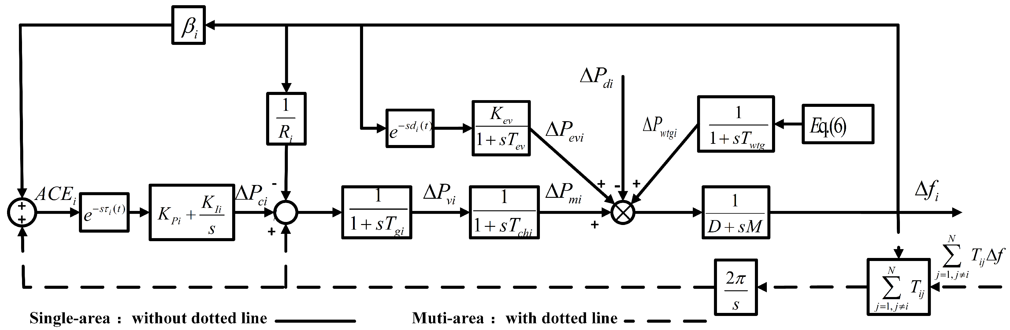
The structure of the delayed LFC system is shown in Figure 1. The model of the EVA for the frequency regulation is described by
Δ P ev = K ev 1 + s T ev
By aggregating numerous individual EVs into an EVA as described in (4), the LFC controller can treat these distributed EV resources as an equivalent collective regulation unit, thereby avoiding a significant increase in the system dimension and computational burden [19]. The communication delay associated with EV participation is modeled as a common equivalent delay in the EVA channel [20].
The differential equation of the wind turbine generator (WTG) can be expressed as
Δ P ˙ w t g = 1 T w t g Δ P w t g + 1 T w t g Δ P w
where P w t g and P w represent, respectively, the output power change of WTG and wind power.
According to (3), P w i n d can be obtained by differentiating the probability model:
Δ P w = ( b + 2 b · v ) P r Δ v v c i v v r 0 v r v < v c o v < v c i v v c o
Through (6), within the range of v c i v v r , the relationship between the change in wind power output P w and the change in wind speed Δ v can be obtained. Therefore, in the probability model of wind power output, (5) can be expressed as
Δ P ˙ w t g = 1 T w t g Δ P w t g + ( b + 2 b · v ) P r T w t g Δ v
Then, the i-th area control error ( A C E i ) is
A C E i = β i Δ f i + Δ P t i e i , e
and a PI-type LFC controller is designed by
u i ( t ) = K P i A C E i ( t ) K I i A C E i ( t ) d t
where K P i denotes the proportional coefficient and K I i denotes the integral coefficient.
The system state vector is defined as x ( t ) = col { Δ f i , Δ P e v i , Δ P w t g i , Δ P m i , Δ P v i , A C E i , Δ P tie i } , ω i ( t ) = col { Δ P d i , Δ v i } , z i ( t ) = Δ f i . Then, the multi-area LFC system can be written as the following closed-loop model:
{ x ̇ ( t ) = A x ( t ) + i = 1 N A di x t τ i + F ω z ( t ) = C z x ( t )
where
x ( t ) = col x 1 ( t ) , x 2 ( t ) , , x n ( t ) ω ( t ) = col ω 1 ( t ) , ω 2 ( t ) , , ω N ( t ) z ( t ) = diag z 1 ( t ) , z 2 ( t ) , , z n ( t ) A = A 11 A 1 n A n 1 A n n , A i j = 0 6 × 1 0 6 × 6 2 π T i j 0 1 × 6 A d i = diag 0 , , A d i i , , 0 A d i i = col 0 1 × 7 , B 1 , 0 2 × 7 , B 2 , 0 2 × 7 B 1 = K e v i T e v i 0 1 × 6 , B 2 = K P i β T g 0 1 × 4 K I i T g i K P i T g i A i i = D i M i 1 M i 1 M i 1 M i 0 0 1 M i 0 1 T e v i 0 0 0 0 0 0 0 1 T w t g i 0 0 0 0 0 0 0 1 T c h i 1 T c h i 0 0 1 R T g i 0 0 0 1 T c h i 0 0 β 0 0 0 0 0 1 a 0 0 0 0 0 0 a = 2 π j = 1 , j i N T i j F = d i a g { F 1 , F 1 , F N } F i = 1 M 0 0 0 0 0 0 0 K W T w t g 0 0 0 T , C z = 1 0 5 × 1 T
Furthermore, a model reconstruction technique [21] is adopted. By separating the state without delay from all other states, the original model (10) is transformed into a coupled system, which is restructured as follows:
x ˙ 1 ( t ) = A 11 x 1 ( t ) + A 12 x 2 ( t ) + F 11 ω 1 ( t ) x ˙ 2 ( t ) = A 21 x 1 ( t ) + A 22 x 2 ( t ) + A d x 2 ( t ) + F 12 ω 2 ( t ) z ( t ) = C ˜ z x 1 ( t )
where
A d = i = 1 N A ˜ di x t τ i x 1 i ( t ) = col { Δ f i , ACE i , Δ P tie i } x 2 i ( t ) = col { Δ P e v i , Δ P w t g i , Δ P m i , Δ P v i } ω 1 i ( t ) = Δ P d i , ω 2 i ( t ) = Δ v i x 1 = col { x 11 , x 12 , x 1 N } x 2 = col { x 21 , x 22 , x 2 N } ω 1 ( t ) = col { ω 11 ( t ) , ω 12 ( t ) , ω 1 N ( t ) } ω 2 ( t ) = col { ω 21 ( t ) , ω 22 ( t ) , ω 2 N ( t ) } A 11 A 12 A 21 A 22 = T A T 1 , 0 0 A ˜ d i 0 = T A d i T 1 F 11 0 0 0 0 0 F 12 0 = T F 0 T 1 C ˜ z 0 0 0 = T C z 0 T 1 T = E a 1 , E a 2 , , E a n 1 , E b 1 , E b 2 , , E b n 2 T E k = 0 1 × ( k 1 ) , 1 , 0 1 × ( n 1 + n 2 k ) T
where E a k represents the number of non-zero columns of A d , and E b k represents the number of other columns.
Remark 2.
The basic idea of the model reconstruction technique is to exploit the sparse structure of the delayed LFC model. In the original system, not all state variables appear directly in the delayed term. Therefore, the state vector is reordered according to the non-zero columns of the delayed-state matrix. The states directly involved in the delayed feedback channel are collected as x 1 ( t ) , while the remaining delay-free states are collected as x 2 ( t ) . By using a nonsingular transition matrix T, the original state vector is transformed into [ x 1 T ( t ) , x 2 T ( t ) ] T = T x ( t ) . This transformation does not change the system dynamics but converts the original model into an equivalent coupled form consisting of a delay-related subsystem and a delay-free subsystem. The reconstruction procedure can be briefly summarized as follows. Step 1: the delay-related states are identified from the nonzero columns of the delay matrix A d = i = 1 N A d i . Step 2: a nonsingular transition matrix T is constructed to reorder the original state vector as [ x 1 T ( t ) , x 2 T ( t ) ] T = T x ( t ) , where x 1 ( t ) contains the delay-related states and x 2 ( t ) contains the remaining states. Step 3: the system matrices are transformed by T A T 1 . The other matrices can be obtained in a similar way. It should be noted that, compared with the model before reconstruction, the reconstructed model may lead to a very slight loss in the subsequent RPI calculation accuracy. This loss is not caused by the equivalent state transformation, but mainly results from the reduced-order LKF construction, where fewer delay-dependent terms and a lower number of decision variables (NDV) are introduced into the LMI conditions.
Remark 3.
In this study, the delays in the LFC signal and EV signal transmission channels are described by a common time-varying delay upper bound. This treatment does not imply that the two physical communication paths are identical. When the detailed EV communication structure is unavailable, the common bound can represent the worst-case delay effect of the involved transmission channels, so that the derived stability condition and RPI provide a conservative guarantee if the actual delays remain below this bound. If the effects of heterogeneous delays need to be further distinguished, the present model can be extended to a multi-delay LFC formulation together with a corresponding multi-delay LKF [22]. In this case, the delayed states associated with the LFC signal and EV control signal are separately described by x ( t τ L F C ( t ) ) and x ( t τ E V ( t ) ) , respectively, and the system dynamics can be written as x ˙ ( t ) = A x ( t ) + A L F C x ( t τ L F C ( t ) ) + A E V x ( t τ E V ( t ) ) + F ω ( t ) . Here, τ L F C ( t ) and τ E V ( t ) denote the independent transmission delays of the LFC and EV control channels. Accordingly, the RPI can be expressed as γ = γ ( h L F C , h E V , μ L F C , μ E V ) , so that the robustness degradation caused by each transmission channel can be analyzed separately.

2.3. Objective

This paper investigates the co-design of robust controllers for a delayed load frequency control system that incorporates uncertain wind power and EVs. This includes the robust performance evaluation of the system and the optimization of the controller gains. The problem can be described as follows: for the preset delay upper bound, suitable controller gains are found to ensure that the closed-loop system is stable without disturbance under any delay less than the given delay upper bound, and to minimize the effect of disturbance ω ( t ) on the controlled output z ( t ) , defined as RPI and denoted by γ , z ( t ) 2 w ( t ) 2 < γ .

3. H Performance Analysis and Controller Co-Design of LFC System

This section presents a method applicable for calculating the H performance index of the LFC system. Based on the derived RPI, controllers can be co-designed to enhance system robustness under both time delays and wind power uncertainty.

3.1. H Performance Analysis

Theorem 1.
For given scalars τ 1 and τ 2 , system in (10) satisfying (12) is asymptotically stable if there exist positive-definite matrices P R 5 n × 5 n , Q i R n × n ,   i = 1 , 2 , Q 3 R 4 n × 4 n , R i R n × n ,   i = 1 , 2 along with matrices T 1 R ( 14 n + 2 ) × n , T i R 9 n × n ,   i = 3 , 4 , 5 ,   M i R 3 n × 14 n + 2 ,   i = 1 , 2 , such that the following LMI (12) holds:
i = 1 3 Υ i + Υ 5 ( τ j ) τ 12 M k T Θ 2 < 0 , j , k { 1 , 2 } , j k
where
Υ 1 = Sym C 1 T P C 11 Υ 2 = e 1 T Q 1 e 1 e 2 T Q 1 e 2 + e 1 T Q 2 e 1 ( 1 μ ) e 3 T Q 2 e 3 + C 21 T Q 3 C 21 C 22 T Q 3 C 22 + Sym C 23 T Q 3 C 24 Υ 3 = e s T ( τ 1 2 R 1 + τ 12 2 R 2 ) e s C 31 T Γ T Θ 1 Γ C 31 + τ 12 Sym ( C 32 T Γ T M 1 + C 33 T Γ T M 2 ) Υ 4 = e 1 T C z T C z e 1 γ 2 e 15 T e 15 Υ 5 ( τ ( t ) ) = Sym T 1 σ 1 ( τ ( t ) ) + i = 3 5 λ i T T i σ i ( τ ( t ) )
and
C 1 = col { e 1 T τ 1 e 5 T e 13 T τ 1 2 e 6 T τ 1 t e 7 T + τ t 2 ( e 9 T + e 11 T ) } C 11 = col { e s T ( e 1 e 2 ) T ( e 2 e 4 ) T τ 1 ( e 1 e 5 ) T ( τ 12 e 2 e 13 ) T } C 21 = col { e 2 T e 1 T 0 14 n × n e 13 T } C 22 = col { e 4 T e 1 T e 13 T 0 14 n × n } C 23 = col { e 13 T τ 12 e 1 T τ 1 t e 7 T + τ t 2 ( e 9 T + e 11 T ) τ 12 e 13 T τ 1 t e 7 T + τ t 2 ( e 9 T + e 11 T ) } C 24 = col { 0 14 n × n e s T e 2 T e 4 T } C 31 = col { e 1 T e 2 T e 5 T e 6 T } C 32 = col { e 2 T e 3 T e 12 T e 8 T } C 33 = col { e 3 T e 4 T e 14 T e 10 T } Θ i = diag { R i , 3 R i , 5 R i } , i = 1 , 2 σ 1 ( τ ( t ) ) = e 13 τ 1 t e 12 τ t 2 e 14 σ 3 ( τ ( t ) ) = e 7 τ 1 t e 8 σ 4 ( τ ( t ) ) = e 9 τ t 2 e 10 σ 5 ( τ ( t ) ) = e 11 τ 1 t e 12 λ i = { λ 1 T e 2 i + 1 T e 12 T e 13 T e 14 T } , i = 3 , 4 , 5 λ 1 = col { e ¯ 1 T e ¯ 2 T e ¯ 3 T e ¯ 4 T e ¯ 5 T } τ 12 = τ 2 τ 1 , τ t 2 = τ 2 τ ( t ) , τ 1 t = τ ( t ) τ 1 Γ = I I 0 0 I I 2 I 0 I I 6 I 12 I
e s = A e 1 + A d e 3 + F e 15 e i = 0 n × ( i 1 ) n I n 0 n × ( 14 1 ) n 0 n × n 3 , i = 1 , 2 , , 14 e 15 = 0 n 3 × 14 n I n 3
Proof: Refer to Appendix A.
Theorem 2.
For given scalars τ 1 and τ 2 , system in (11) satisfying (13) is asymptotically stable if there exist positive-definite matrices P ¯ R ( 5 n 1 + n 2 ) × ( 5 n 1 + n 2 ) , Q ¯ i R n 1 × n 1 , i = 1 , 2 , Q ¯ 3 R 4 n 1 × 4 n 1 , R ¯ i R n 1 × n 1 , i = 1 , 2 along with matrices T ¯ 1 R ( 14 n 1 + n 2 + 2 ) × n 1 , T ¯ i R 9 n 1 × n 1 , i = 3 , 4 , 5 , M ¯ i R 3 n 1 × ( 14 n 1 + n 2 + 2 ) , i = 1 , 2 , such that the following LMI (13) holds:
i = 1 3 Υ ¯ i + Υ ¯ 5 ( τ j ) τ 12 M ¯ k T Θ ¯ 2 < 0 , j , k { 1 , 2 } , j k
where
Υ ¯ 1 = Sym C ¯ 1 T P ¯ C 11 ¯ Υ ¯ 2 = e ¯ 1 T Q ¯ 1 e ¯ 1 e ¯ 2 T Q ¯ 1 e ¯ 2 + e ¯ 1 T Q ¯ 2 e ¯ 1 ( 1 μ ) e ¯ 3 T Q ¯ 2 e ¯ 3 + C ¯ 21 T Q ¯ 3 C ¯ 21 C ¯ 22 T Q ¯ 3 C ¯ 22 + Sym C ¯ 23 T Q ¯ 3 C ¯ 24 Υ ¯ 3 = e ¯ s 1 T ( τ 1 2 R ¯ 1 + τ 12 2 R ¯ 2 ) e ¯ s 1 C ¯ 31 T Γ T Θ ¯ 1 Γ C ¯ 31 + τ 12 Sym ( C ¯ 32 T Γ T M ¯ 1 + C ¯ 33 T Γ T M ¯ 2 ) Υ 4 = e 1 T C z T C z e 1 γ 2 e 16 T e 16 γ 2 e 17 T e 17 Υ ¯ 5 ( τ ( t ) ) = Sym T ¯ 1 σ ¯ 1 ( τ ( t ) ) + i = 3 5 λ ¯ i T T ¯ i σ ¯ i ( τ ( t ) )
and
F 11 = col { e s 1 T ( e ¯ 1 e ¯ 2 ) T ( e ¯ 2 e ¯ 4 ) T τ 1 ( e ¯ 1 e ¯ 5 ) T ( τ 12 e ¯ 2 e ¯ 13 ) T e s 2 T } e s 1 = A 11 e ¯ 1 + A 12 e ¯ 15 F 11 e 16 ¯ e s 2 = A 21 e ¯ 1 + A 22 e ¯ 15 + A ^ d e ¯ 3 + F 12 e 11 ¯ e ¯ i = 0 n 1 × ( i 1 ) n 1 I n 1 0 n 1 × ( 14 i ) n 1 0 n 1 × ( n 2 + n 3 ) , i = 1 , 2 , , 14 e ¯ 15 = 0 n 2 × 14 n 1 I n 2 0 n 2 × n 3 e ¯ 16 = 0 n 31 × ( 14 n 1 + n 2 ) I n 31 0 n 31 × n 32 e ¯ 17 = 0 n 32 × ( 14 n 1 + n 2 + n 31 ) I n 32
To avoid redundant expressions, the matrix ( C i ¯ , σ ¯ i and λ ¯ i ) has the same structure as that in Theorem 1 ( C i , σ i and λ i ), except that it is represented by the new basis vector ( e ˜ i ). The proof is similar to that of Theorem 1 in Appendix A, with x ( t ) in the LKF and ψ ( t ) replaced by x 1 ( t ) , and x 2 ( t ) appended as the last row of ψ ( t ) ; thus, it is omitted for space limitation. Based on the LMI conditions in Theorems 1 and 2, the RPI γ can be calculated by a binary search procedure, as summarized in Algorithm 1.
Remark 4.
In this study, the PI-type LFC model is formulated under a linearized operating condition, and nonlinear physical constraints such as governor rate constraint (GRC), governor dead band (GDB), turbine valve position limits, and actuator saturation are not explicitly included. This treatment is adopted to keep the RPI-based LKF analysis and GA-PSO controller co-design tractable, and to focus on the effects of wind power uncertainty and communication delays. It should be noted that such nonlinearities may reduce the effective control action, increase the obtained RPI γ, and lead to more conservative admissible delay margins. Several existing methods can be used to incorporate these nonlinear factors into LFC analysis. For example, valve position limits can be represented by a Takagi–Sugeno (T–S) fuzzy model, where the nonlinear dynamics are approximated by the convex combination of local linear models [23], and GDB, GRC, reheater dynamics, and time-delay effects can also be handled by optimization-based fuzzy PID controllers, such as hybrid firefly algorithm–pattern search methods [24]. Therefore, although these nonlinear constraints are not the main focus of the present work, the proposed RPI-based framework can be further extended by combining T–S fuzzy modeling and intelligent optimization techniques.
Remark 5.
By separating the states related to time delay from those not related to time delay, a more computationally efficient stability condition can be obtained. Just as stated in Theorem 2, the NDV is 147.5 n 1 2 + 12 n 1 n 2 + 0.5 n 2 2 + 20.5 n 1 + 0.5 n 2 . Before model reconstruction, the NDV is 147.5 n 2 + 20.5 n , where n = n 1 + n 2 , n 1 is the amount of delay-related variables and n 2 is the amount of delay-free variables. It can be seen that the variables that need to be calculated mainly depend on the size of n 1 , and are much smaller than n 1 + n 2 .
Algorithm 1 The binary search algorithm for the RPI γ in the LFC system
  • Step 1: Given the system parameters and the PI controller gains.
  • Step 2: Solve for the RPI γ .
     1.
    A set of system delay upper bound h. Specify the appropriate search range [ γ max , γ min ] with γ min = 0 and γ max to be big enough. Set the proper precision γ a = 0.0001 ;
     2.
    By examining LMIs (12) or (13), determine whether the system is stable under the given γ test = ( γ max + γ min ) / 2 ;
     3.
    if LMIs (12) or (13) is feasible, then set γ max = γ test ; else, set γ min = γ test ;
     4.
    end if
     5.
    if  | γ max γ min |   < γ a , then set γ = γ max ; else, repeat 2);
     6.
    end if
     7.
    Return  γ .
  • Step 3: Output the minimum RPI γ .

3.2. Frequency Controller Design Based on RPI

The GA-PSO algorithm combines the efficient convergence of particle swarm optimization with the strong global exploration ability of genetic algorithms. In this approach, the swarm of particles represents the population of candidate controller gain vectors. Each particle’s position encodes a specific set of controller parameters. The RPI (robust performance index) acts as the fitness function, i.e., f ( X i k ) = γ ( X i k ) . The algorithm drives the swarm to collectively search for the globally optimal controller gains that minimize the RPI. The following outlines the procedure for controller co-design using the GA-PSO methodology.
Set the position vector X i = [ K p , K I ] of each particle to characterize a complete set of controller parameters. Within the given parameter feasible region, randomly initialize a population consisting of N particles.
Each particle updates its velocity V i and position X i based on its individual historical best position p b e s t i and the global best position g b e s t of the swarm:
V i ( k + 1 ) = ω V i ( k ) + c 1 r 1 p b e s t i k X i k
+ c 2 r 2 g b e s t k X i k
X i ( k + 1 ) = X i ( k ) + V i ( k + 1 )
where k is the iteration number, ω is the inertia weight, c 1 , c 2 are the learning factors, and r 1 , r 2 are random numbers within [ 0 , 1 ] .
As particles converge around g b e s t k , the terms ( p b e s t i k X i k ) and ( g b e s t k X i k ) diminish, causing the velocity update to approach zero. This leads to stagnation, where the swarm becomes trapped and cannot escape the current region. If g b e s t k is only a local optimum, early convergence to it results in premature stagnation. To suppress premature convergence and improve the ability to escape local optima, this paper embeds genetic operator selection, crossover, mutation, and substitution after each update. This forms the outer search strategy of GA-PSO. In this step, particles with better fitness values are selected from the current population as parents for subsequent genetic operations.
Pair the selected parent particles in pairs and cross them with a certain probability P c to generate offspring particles, which can be expressed as
X child 1 k = α · X parent 1 k + ( 1 α ) · X parent 2 k X child 2 k = ( 1 α ) · X parent 1 k + α · X parent 2 k
Randomly perturb the positions of the crossed particles with a relatively low probability P m to form Gaussian variation
X child k = X child k + σ N ( 0 , 1 )
The new offspring generated by GA is injected into the population to replace several of the worst particles.
X i ( k ) X child k
Then, continue pressing (14) and (15).
For a given allowable time-delay range [ τ 1 , τ 2 ] , Algorithm 2 is described to design the controllers with the required robustness. The GA-PSO is employed to systematically determine the optimal controller gains by minimizing the RPI γ , where a smaller γ value directly corresponds to enhanced LFC system robustness. The optimization process is constrained by the H stability conditions stated in Theorem 1, requiring the controller gains to satisfy LMIs (9) and (10) under specified delay conditions.
Algorithm 2 Design of LFC system Control Scheme
  • Step 1: Establish the LFC system control model.
  • Step 2: Use GA-PSO to find the controller gain that makes the LFC system have the minimum γ .
     1.
    Set the parameters of the GA-PSO algorithm (population size, maximum iterations, crossover/mutation probabilities, inertia weight) and initialize the particle population.
     2.
    Use the RPI from Algorithm 1 as the objective function, evaluate each fitness of particle (i.e., γ ), and update the personal best (pbest) and global best (gbest) positions.
     3.
    Perform selection, crossover, and mutation to generate a new GA population. Merge elite PSO particles with the new GA individuals to form the next generation.
     4.
    Repeat step until the maximum iterations are reached or convergence criteria are met.
     5.
    Output the controller gains corresponding to the global best position.
  • Step 3: Bring the controller gains into the controllers, set up the simulation environment, and test.

4. Case Studies

In this section, case studies are conducted based on a single-area LFC scheme and a two-area LFC scheme to demonstrate the effectiveness and superiority of the proposed method. The parameters of the LFC system are shown in Table 1. It is assumed that the delay within each area is the same. In the case studies, numerical calculations and simulation tests are based on the Yalmip toolbox and Simulink in MATLAB 2022b, respectively.
The GA-PSO algorithm is partially initialized with the following parameters. Set position bounds, X m i n = 1 , X m a x = 1 , V m i n = 0.3 , V m a x = 0.3 , ω m i n = 0.3 , ω m a x = 0.3 , p c = 0.8 and p m = 0.1 , population size N = 20 , and the maximal iteration times K m a x = 20 . For a fair comparison, the baseline controllers without considering wind power uncertainty are tuned using the same optimization framework and parameter-tuning procedure as the proposed controllers. The only difference lies in the wind turbine model used during the controller optimization process. Specifically, for the baseline controllers, a simplified wind turbine model with Δ P wtgi = 1 1 + s T wtg Δ P w is adopted, and the wind power uncertainty characterized by (3) and (6) is not incorporated.
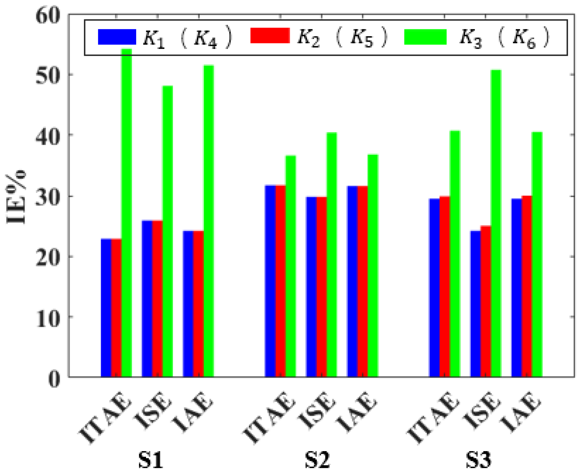
For the following scenario, three control performance indicators are introduced to analyze the robustness of the system: the integral of time multiplied absolute value of the error ( ITAE = 0 t s t Δ f ) , the integral of squared error ( ISE = 0 t s ( Δ f ) 2 d u ) , the integral of absolute error ( IAE = 0 t s Δ f d u ) . Then, to better compare the performance of different controllers, these indexes are uniformly defined as IE, with I E % ( K 1 / 2 / 3 ) = I E ( K 1 / 2 / 3 ) / I E ( K 1 ) + I E ( K 2 + I E ( K 3 ) or I E % ( K 1 / 2 ) = I E ( K 1 / 2 ) / I E ( K 1 ) + I E ( K 2 .

4.1. Case Studies on the Single-Area LFC System

This part focuses on the implementation of the proposed method in a single-area LFC system. It specifically examines the impact on the robustness performance of the system when the wind speed is uncertain, as well as evaluating the controller performance.

4.1.1. Numerical Calculation

Table 2 presents the results of how different communication delay times affect the robustness performance index of the single-area LFC system under a wind speed of 5. It quantitatively measures the impact of increasing delay on the disturbance suppression ability of the system. The results show that the RPI always increases with the increase in the time delay, indicating that the increase in time delay reduces the robustness of the system. Furthermore, from Table 3 and Table 4, it can be concluded that Theorem 2 significantly enhances the computational efficiency compared to Theorem 1, while sacrificing only a small amount of accuracy.
To quantify the impact of this core uncertainty of wind speed fluctuations on the disturbance resistance of system, based on the segmented model of wind power output established in Section 2, three characteristic wind speed operating intervals were defined. Here, only the wind speed within the range between the cut-in wind speed and the cut-out wind speed is considered. The delay range is set as [ τ 1 , τ 2 ] = [ 0 , 1 ] . The corresponding RPI for different situations is shown in Table 3. This verifies that as the wind power output increases, it poses a severe challenge to the robustness of the system as a persistent disturbance source.

4.1.2. Simulation Test

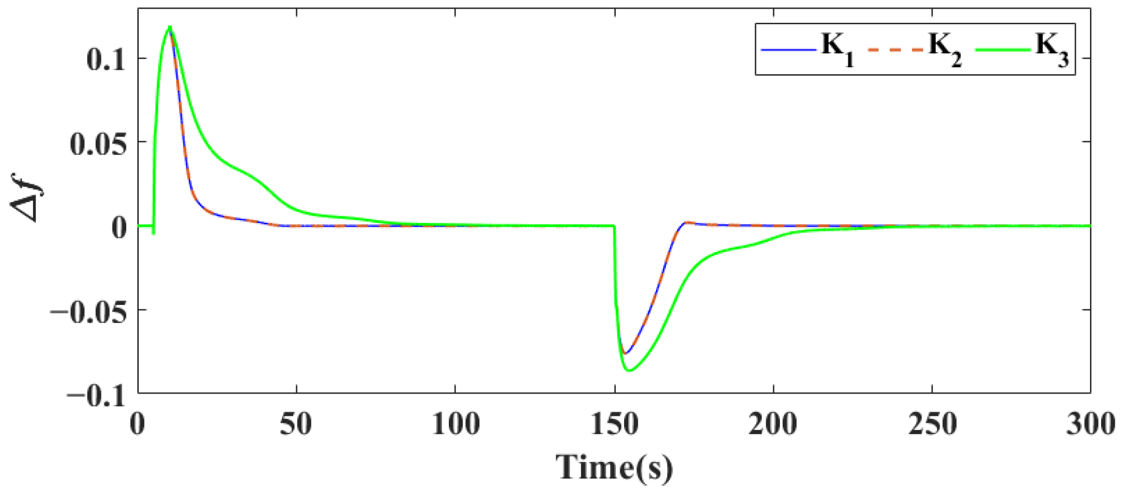
To examine the sensitivity of the GA-PSO optimization to the initial population size and the maximum number of iterations, different [ N , K max ] configurations were tested, as listed in Table 5. The optimized gains become unchanged when K max = 20 and the population size is further increased from N = 20 to N = 30 , suggesting that the obtained solution is insensitive to further population enlargement and that premature convergence is unlikely within the tested search settings. Considering that the single-area LFC system is affected by a time delay of up to 5 s and a maximum wind speed of 5, the controller gains K 1 = [ 0.101 , 0.158 ] and K 2 = [ 0.098 , 0.158 ] can be determined through Theorem 1 and Theorem 2, respectively. K 3 = [ 0.078 , 0.073 ] is determined through Theorem 2 without considering the influence of wind speed.
Scenario 1 (S1) considers a step load disturbance of 0.25 pu occurring at t = 5 s, which decreases to 0.05 pu at t = 150 s. There is a periodic delay as d ( t ) = 5 sin t / 10 + 5 . The frequency response under these conditions is shown in Figure 2.
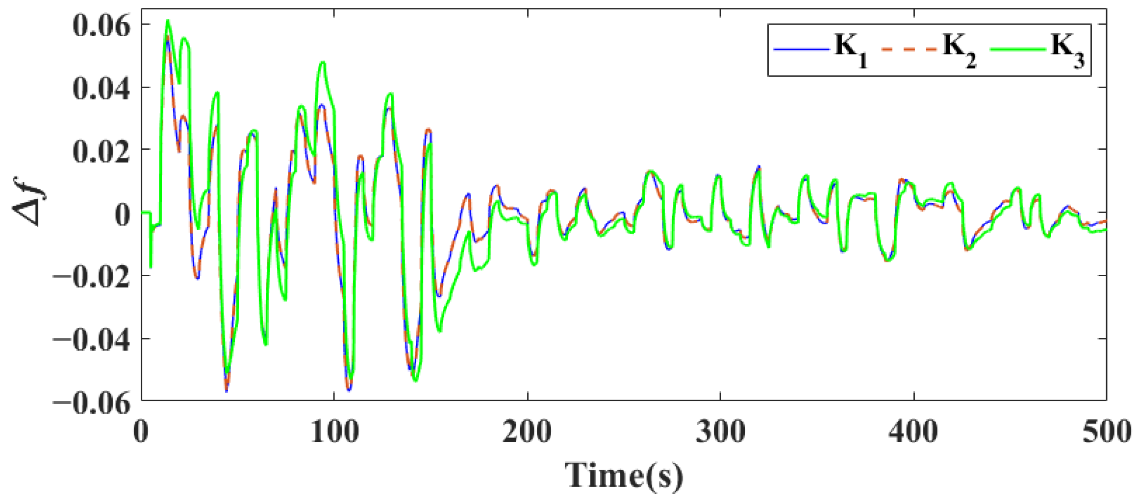
In Scenario 2 (S2), the load disturbance is set such that a 0.5 pu step response occurs at t = 5 s. Under a wind speed of 5 m/s and random disturbances of wind speed variation Δ v ranging from −0.1 pu to 0.1 pu, the periodic delay is the same as that in Scenario 1. Figure 3 shows the regional frequency response when equipped with controllers K 1 , K 2 , or K 3 .
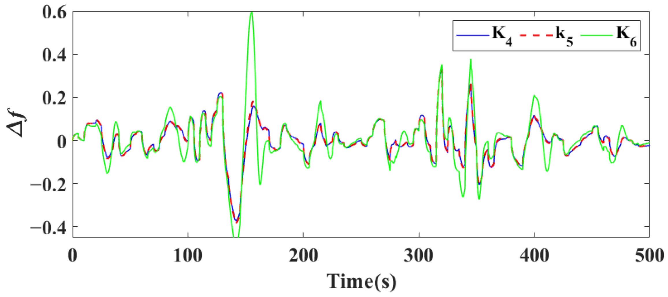
Considering that the single-area LFC system is affected by a time delay of up to 10 s and a maximum wind speed of 10, the controller gains K 4 = [ 0.097 , 0.150 ] and K 5 = [ 0.093 , 0.159 ] can be determined through Theorems 1 and 2, respectively. K 6 = [ 0.072 , 0.282 ] is determined through Theorem 2 without considering the influence of wind speed. Then, set up the following scenario.
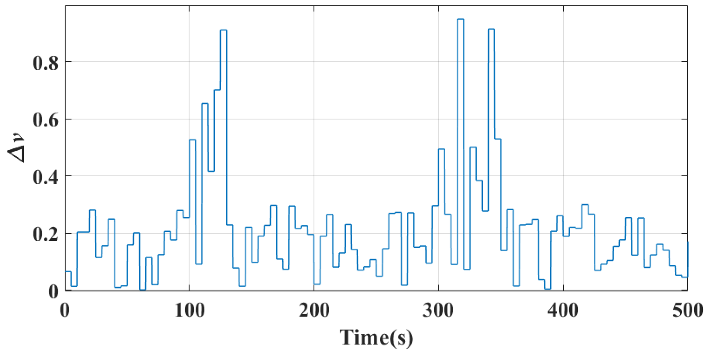
In Scenario 3 (S3), the considered delay is a constant delay of 10 s, and the load disturbance is set such that a 0.25 pu step response occurs at t = 5 s. At a wind speed of 10 m per second, the wind speed variation disturbance is shown in Figure 4. The frequency response under such conditions is illustrated in Figure 5.
A comparison of the results under the three aforementioned scenarios reveals that although all three controllers can ensure stable system operation by driving the frequency deviation response curve to convergence, the systems equipped with controllers K 1 and K 2 exhibit a significantly faster response and relatively smaller deviations compared to those using K 3 . This observation is further supported by the three performance metrics presented in Figure 6. The performances of K 1 and K 2 are highly consistent, indicating that sacrificing a small amount of computational accuracy in exchange for highly efficient results is entirely justified. The results observed in S3 align with those from S1 and S2. Quantitatively, compared with the baseline controllers K 3 and K 6 , the Theorem 1-based controllers K 1 and K 4 and the Theorem 2-based controllers K 2 and K 5 reduce the normalized ITAE, ISE, and IAE indices by approximately 17.4% on average. Therefore, incorporating wind speed uncertainty into the analysis as a necessary consideration for realistic wind conditions can lead to superior frequency deviation performance.

4.1.3. Impact of EV S O C Constraints on Robust Frequency Regulation

To verify the robust frequency-response characteristics of the system when EVs are subject to nonlinear physical constraints imposed by the state of charge, the following formulation is introduced.
K e v , c = K max 1 SOC SOC low SOC max SOC low 2 , Δ f 0 K e v , d = K max 1 SOC SOC high SOC min SOC high 2 , Δ f < 0
where K max denotes the maximum V2G droop gain of the EV aggregator, and S O C max , S O C high , S O C low , and S O C min represent the maximum, high, low, and minimum battery S O C limits, respectively. Accordingly, K e v can be expressed as
K e v = K max K max SOC SOC low ( high ) SOC max ( min ) SOC low ( high ) 2
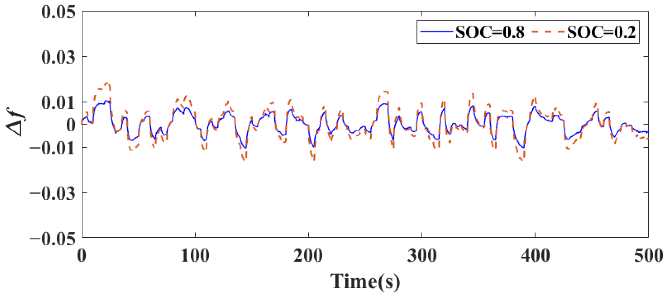
Following the method in [4], two S O C levels, S O C = 0.8 and S O C = 0.1 , are selected for comparison to investigate the sensitivity of the proposed controller to EV S O C constraints. The case of S O C = 0.8 represents sufficient EV regulation capacity, whereas S O C = 0.1 represents a constrained low-SoC condition. The SoC limits are set as S O C max = 0.9 , S O C min = 0.1 , S O C high = 0.8 , and S O C low = 0.2 . According to (17), the corresponding S O C -dependent EV gains in the considered regulation direction are calculated as K e v = 1 for S O C = 0.8 and K e v = 0 for S O C = 0.1 , indicating that the EV frequency-regulation capability is partially depleted under the low- S O C condition. Random load and random wind speed variation disturbances are simultaneously applied to the system, with amplitudes of 0.025 pu and 0.05 pu and sampling times of 3 s and 5 s, respectively. The corresponding frequency responses are shown in Figure 7.
Figure 7 shows the frequency responses under different EV S O C levels. Although S O C = 0.1 represents a constrained low- S O C condition with a partially depleted EV regulation capability, the frequency deviation remains bounded and close to that under S O C = 0.8 . This indicates that the proposed robust controller can tolerate the SoC-dependent variation in the EV gain. Therefore, even when the available EV frequency-regulation capacity is reduced, the closed-loop system can still maintain stable frequency regulation under simultaneous random load and wind speed disturbances.

4.2. Case Studies on the Two-Area LFC System

This part mainly discusses the robust performance of the proposed method in a two-area LFC system, assuming that the delay within each region is the same and that the delay between regions is consistent. In this part, only Theorem 2 was used to calculate the corresponding minimum γ value, which ensures high computational efficiency while still providing a reasonable assessment of robustness, and is applicable for the rapid analysis and design of multi-regional systems.

4.2.1. Numerical Calculation

Table 6 shows the impact of different delays on the RPI of the LFC system in the two-area system. In the calculation, it is assumed that the wind speed is 5. The results show that as the delay increases, the RPI value gradually increases, indicating that the delay has a significant negative impact on the ability of system to suppress disturbances, verifying the weakening effect of delay on the robustness of the multi-region system. Compared with the single-region system, the two-region system has more significant delay sensitivity due to the existence of inter-regional coupling and power interaction through the tie lines.
Table 7 further analyzes the impact of wind speed uncertainty on the robustness of the two regional systems. The calculation results show that as the wind speed increases and the output power of wind power generation rises, the continuous disturbances faced by the system also increase, and the RPI value accordingly rises.
Table 8 and Table 9 further illustrate the relationship between computational time and the number of decision variables. Although the computational burden increases from the single-area case to the two-area case due to the growth of NDVs from 737 to 4306, the model reconstruction technique in Theorem 2 keeps the RPI calculation tractable and significantly improves computational efficiency by reducing the number of delay-related decision variables.

4.2.2. Simulation Test

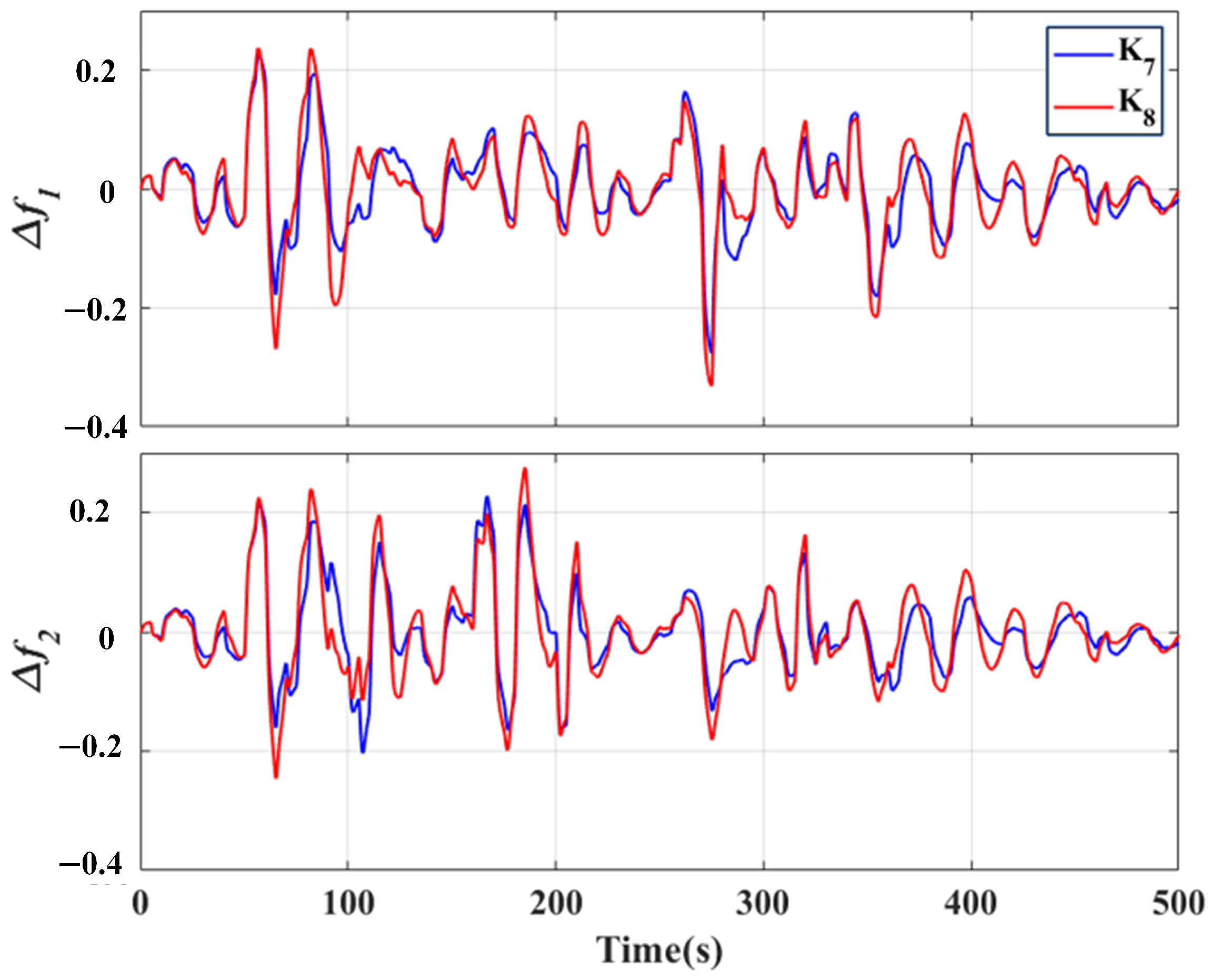
To validate the effectiveness and superiority of the proposed method in this paper, given the 5 s time delay in the dual-region LFC system and the maximum wind speed of 5, the controller gain K 7 = [ 0.018 , 0.113 ] can be determined according to Theorem 2, while K 8 = [ 0.061 , 0.169 ] is also determined by Theorem 2, without considering the influence of wind speed.
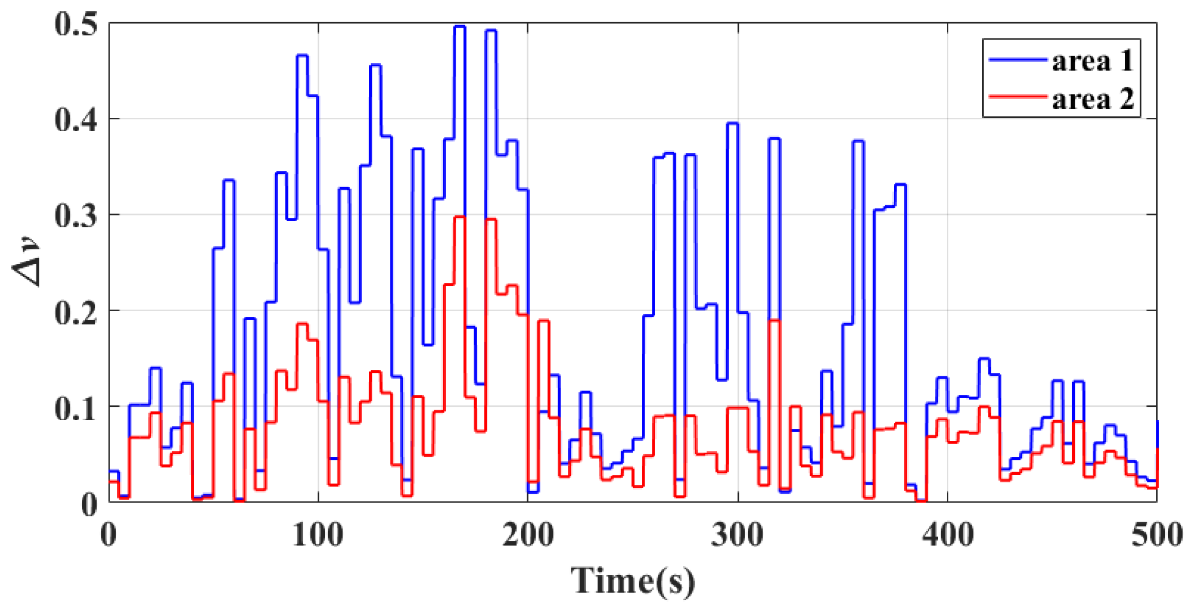
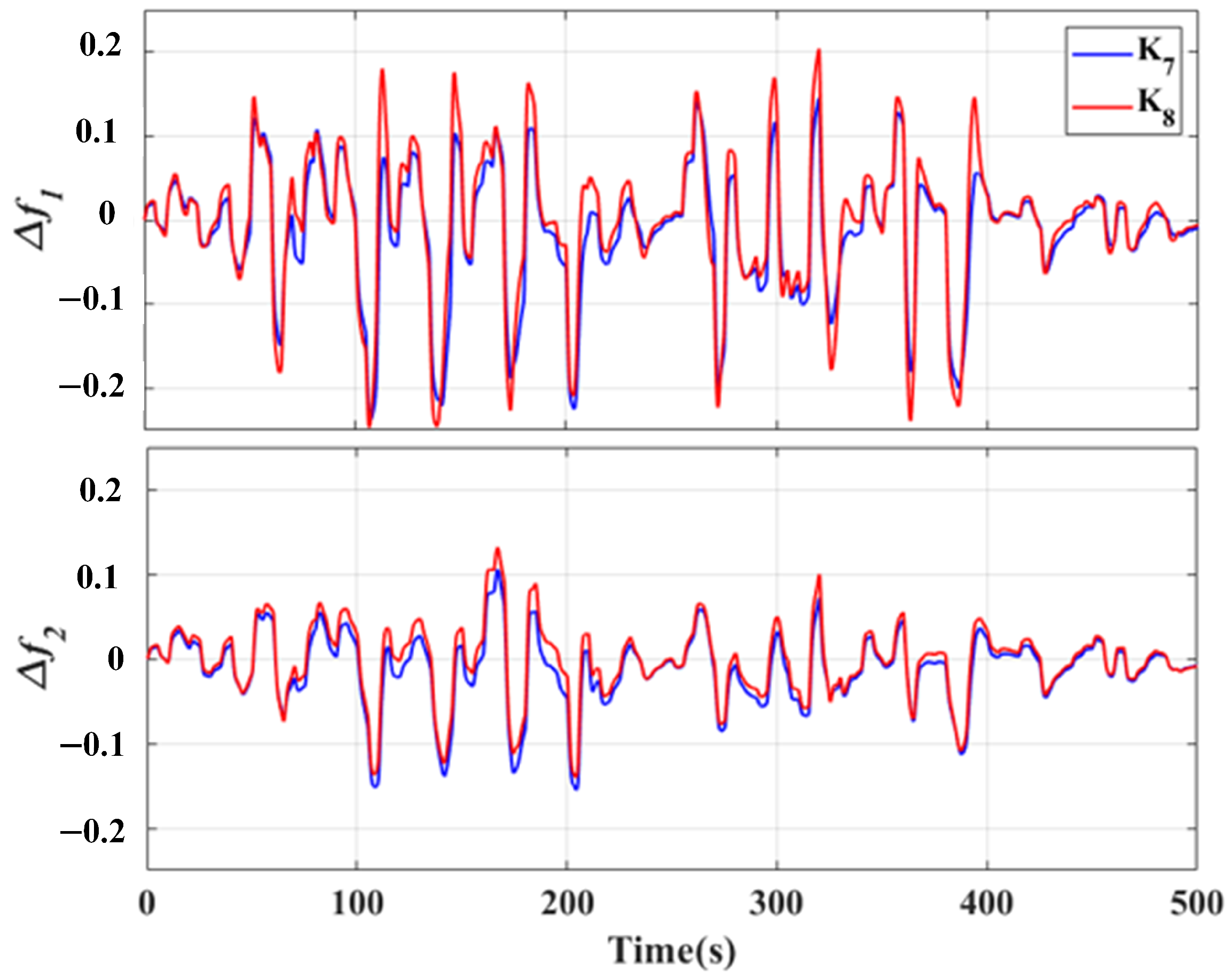
Scenario 4 (S4) assumes that there is a constant 5 s time delay in both regions, and the load disturbance is set such that, at t = 5 s, area 1 generates a 0.2 pu step response, and region 2 generates a 0.25 pu step response. Meanwhile, Figure 8 shows the situation where the wind speed is 5 and there are different wind speed variation disturbances in both regions. The frequency responses under these conditions are shown in Figure 9.
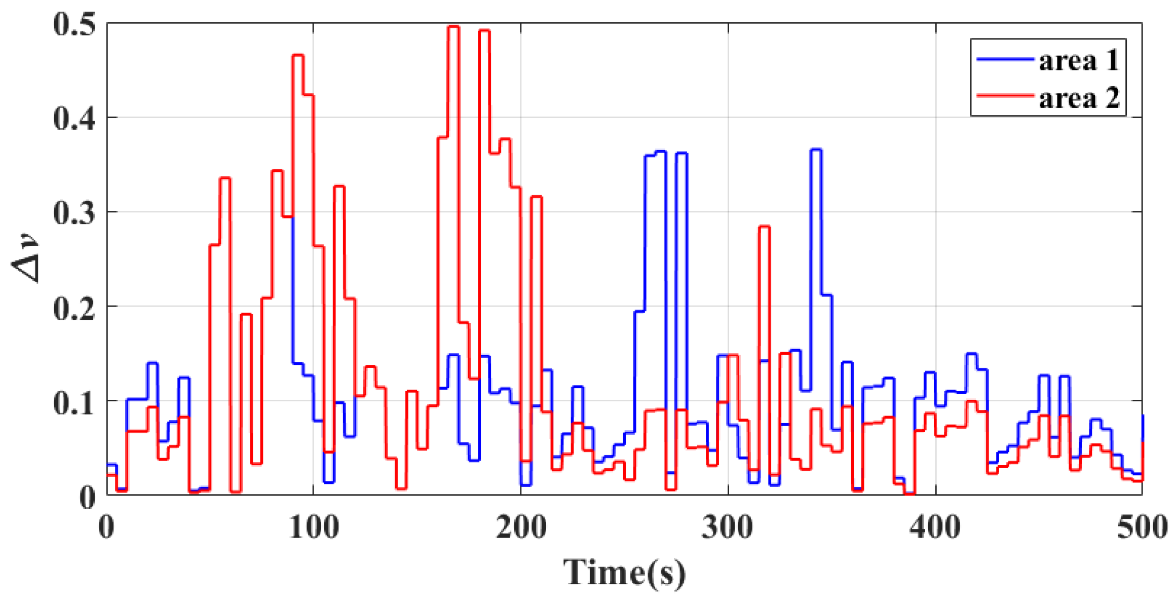
Scenario 5 (S5) assumes that there is a maximum delay of 5 s for both regions, and the periodic delay is d ( t ) = 5 sin t / 10 + 5 . The load disturbance is set as follows: at t = 5 s, region 1 generates a 0.25 pu step response and drops to 0.05 pu at t = 150 s. Region 2 generates a 0.05 pu step response and rises to 0.2 at t = 150 s. Meanwhile, Figure 10 shows the situation where the wind speed is 5 and there are different wind speed variation disturbances in the two regions, aiming to verify the case where there is a significant difference in wind speed changes between the two regions. The frequency responses under these conditions are shown in Figure 11.
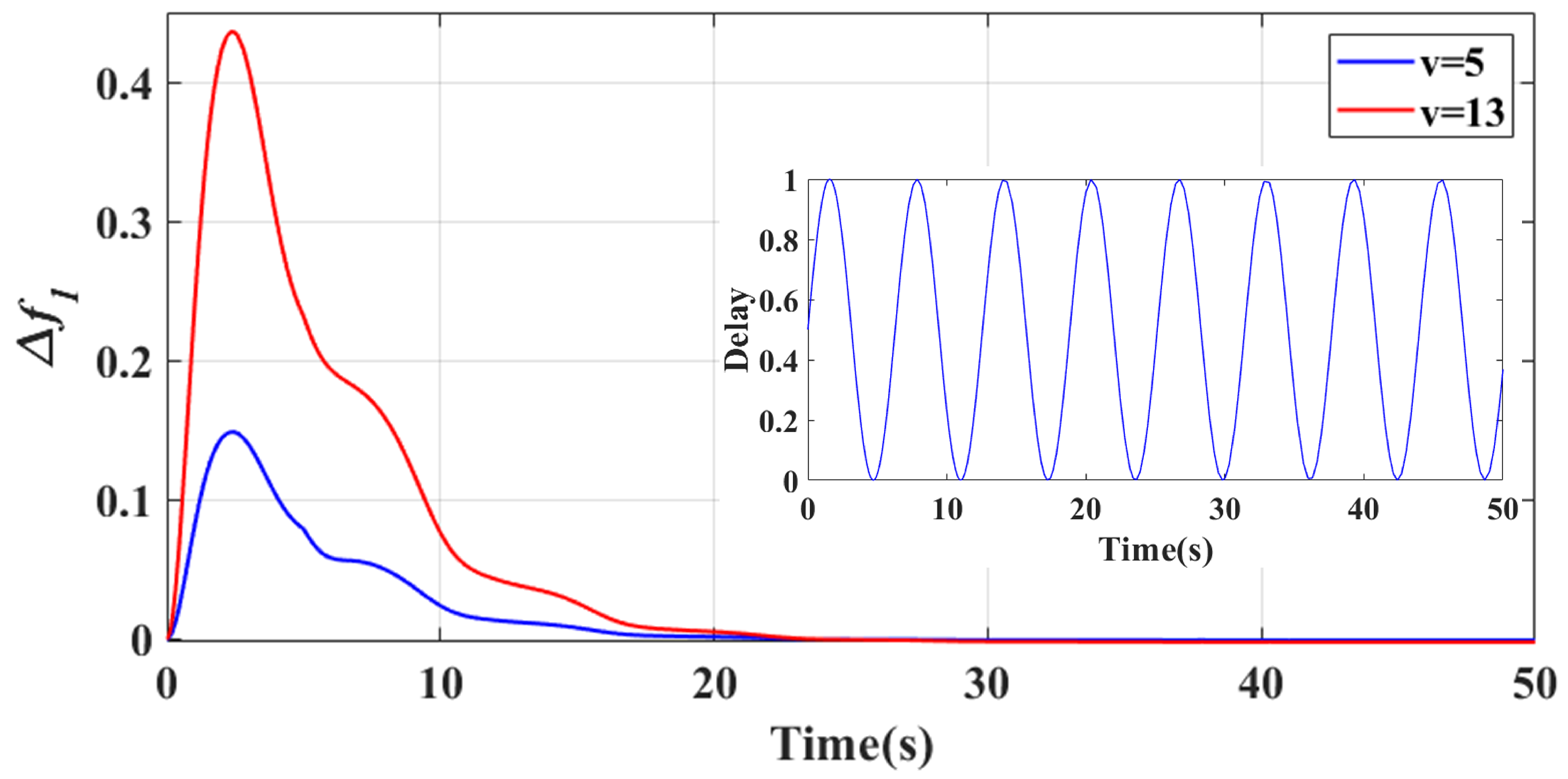
Scenario 6 (S6) is designed to validate the data presented in Table 7. Under identical test conditions, the controller parameters are set to P I = [ 0.1 , 0.2 ] and μ = 0.5 . The system is tested under wind speeds of v = 5 and v = 13 . A load disturbance is implemented as a 0.2 pu step change at t = 5 s. The resulting frequency deviation responses are shown in Figure 12.
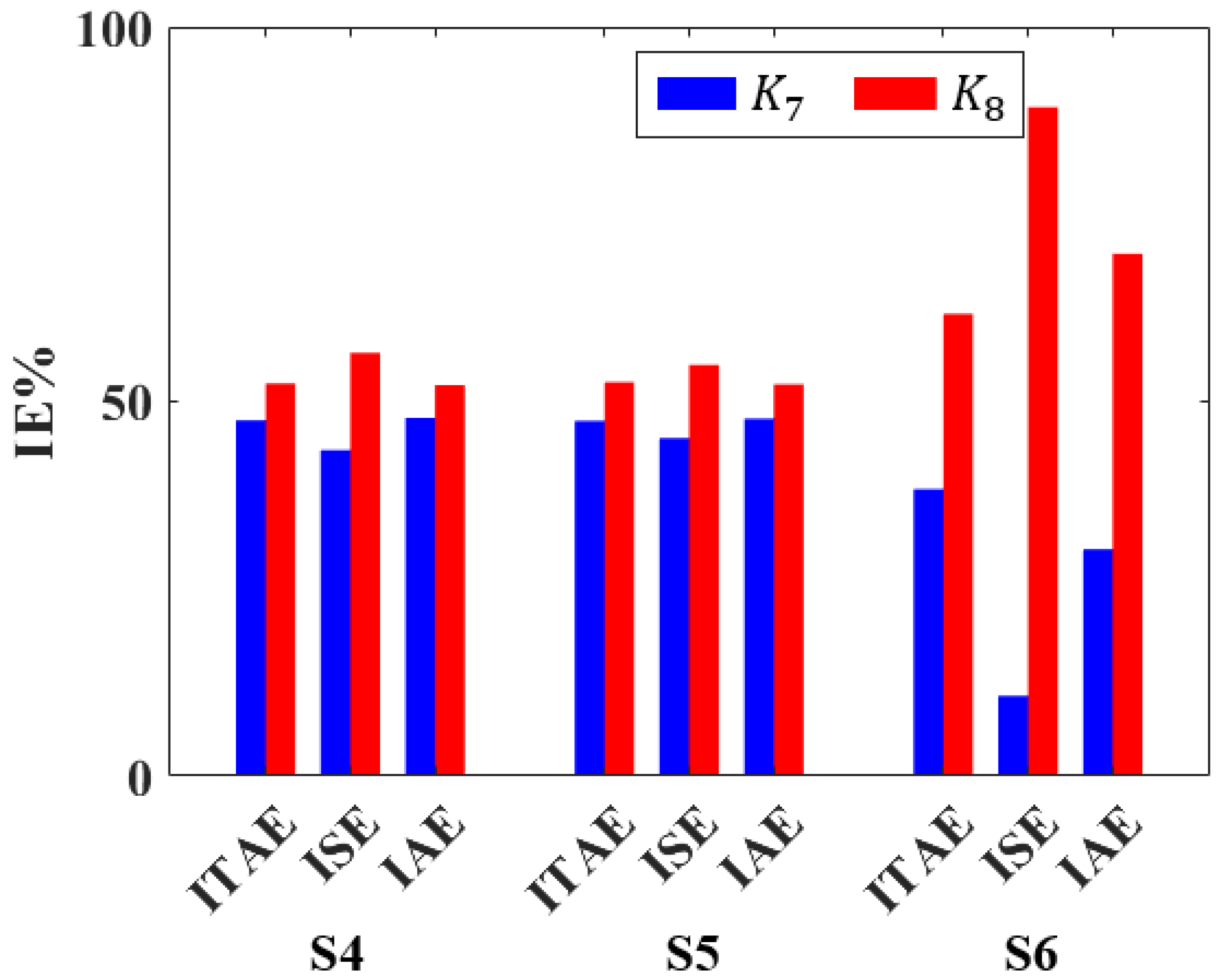
In the more complex and highly coupled two-area system, the proposed controller design method, which integrates GA-PSO optimization with H robust performance analysis, demonstrates excellent scalability, as evidenced by the superior performance of controller K 7 over K 8 further illustrated in Figure 13. In S4 and S5, K 7 reduces the normalized ITAE, ISE, and IAE indices by approximately 9.0% on average compared with the baseline controller K 8 . This approach effectively minimizes the propagation of disturbances between areas and substantially reduces power fluctuations at the tie-line.
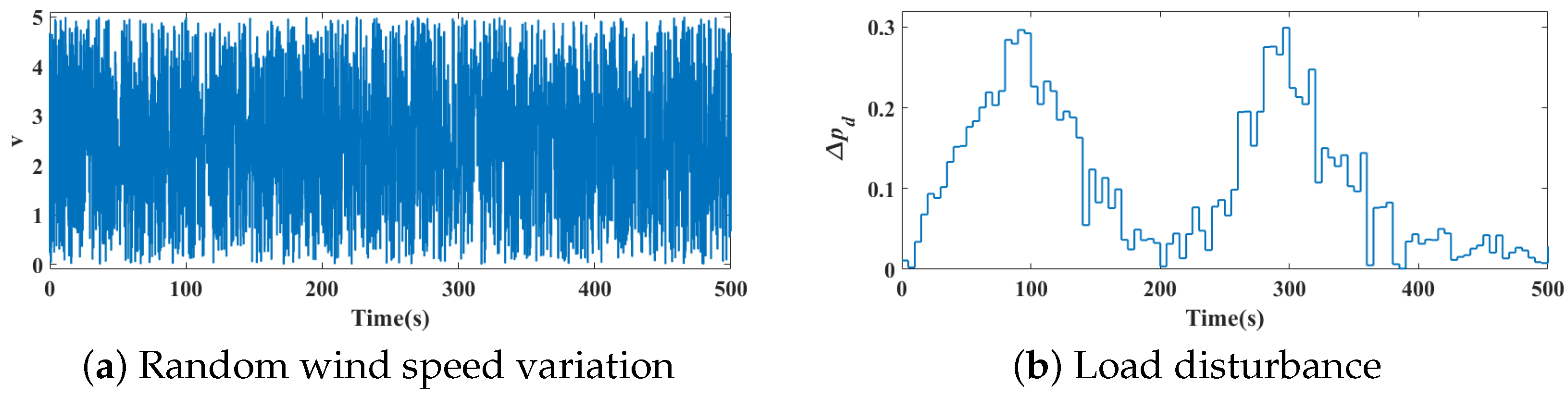
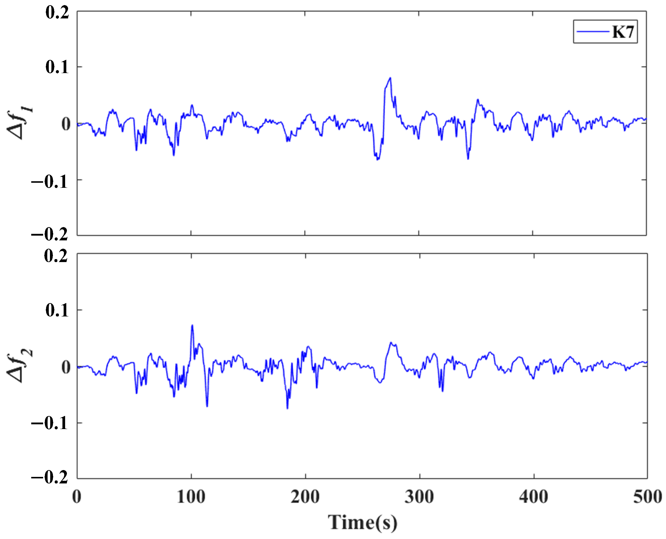
In Scenario 7 (S7), the time delay and Δ v variation are the same as in Scenario 6, while the wind speed undergoes a random variation with a maximum amplitude of 5, as shown in Figure 14a. The load disturbance is presented in Figure 14b. This scenario aims to verify the robust performance of the controller when all disturbances vary simultaneously. The results are shown in Figure 15.
In Scenario 7, where various disturbances vary simultaneously, the designed controller maintains small frequency deviations in both areas, further confirming the robustness of the proposed method under compound disturbances.

5. Conclusions

This paper proposes a robust design framework for LFC systems under wind power uncertainty and communication delays. A segmented wind speed model is established to accurately capture wind power fluctuations, and electric vehicles are incorporated for frequency regulation, forming a realistic multi-area delayed LFC model. The RPI is introduced to quantify system disturbance rejection. Controller parameters are then cooperatively designed by optimizing this index, ensuring stability and performance under specified delays. Case studies confirm that, compared to controllers designed without considering wind uncertainty, the proposed method delivers superior frequency regulation across various wind and delay conditions, effectively suppressing deviations and enhancing system robustness.
Future work will focus on the effects of practical transmission-network and actuator constraints on the RPI. Independent delay upper bounds and delay-jitter rates will be introduced for different signal transmission channels, such as the LFC and EV control paths, to evaluate their impacts on robustness and delay tolerance. Moreover, governor rate constraints, turbine valve limits, and actuator saturation will be incorporated, since neglecting these nonlinear constraints may overestimate the stability margin and disturbance attenuation capability. Extending the proposed framework to heterogeneous-delay and saturation-constrained LFC systems is therefore an important future direction.


Author Contributions

Y.L.: Writing—review & editing, Writing—original draft, Visualization, Methodology, Funding acquisition, Conceptualization. T.W.: Writing—review & editing, Writing—original draft, Validation, Software, Methodology. Y.C.: Writing—review & editing, Supervision, Project administration. J.H.: Supervision, Formal analysis. All authors have read and agreed to the published version of the manuscript.
Funding

This research was funded by the National Natural Science Foundation of China under Grant 62403369; by China Postdoctoral Science Foundation under Grant 2024M752582; by the Postdoctoral Research Project of Shaanxi under Grant 2024BSHTDZZ006; by the Young Talent Fund of Association for Science and Technology in Shaanxi, China, under Grant 20250106; by the Natural Science Foundation of Sichuan Province under Grant 2026NSFSC1515; and by the Natural Science Foundation of Xi’an under Grant 2025JH-ZRKX-0257.

Data Availability Statement

The original contributions presented in this study are included in the article. Further inquiries can be directed to the corresponding author.

Conflicts of Interest

Authors Yantao Lou and Tonghui Wang was employed by the company Xi’an XD Power Systems Co., Ltd. The remaining authors declare that the research was conducted in the absence of any commercial or financial relationships that could be construed as a potential conflict of interest.

Appendix A

Proof of Theorem 1.
Construct the following LKF:
V 1 ( x t ) = ( C 1 ψ ( t ) ) T P ( C 1 ψ ( t ) ) V 2 ( x t ) = t τ 1 t x ( s ) T Q 1 x ( s ) d s + t τ ( t ) t x ( s ) T Q 2 x ( s ) d s + t τ 2 t τ 1 η ( t , s ) T Q 3 η ( t , s ) d s , V 3 ( x t ) = τ 1 t τ 1 t s t x ˙ ( u ) T R 1 x ˙ ( u ) d u d s + τ 12 t τ 2 t τ 1 s t x ˙ ( u ) T R 2 x ˙ ( u ) d u d s ,
where ψ ( t ) = col { ψ 1 ( t ) ψ 2 ( t ) ) · · · ψ 16 ( t ) } , ψ 1 = x ( t )
ψ 2 ( t ) = x ( t τ 1 ) , ψ 3 ( t ) = x ( t τ ( t ) ) , ψ 4 ( t ) = x ( t τ 2 ) ψ 5 ( t ) = 1 τ 1 t τ 1 t x ( s ) d s , ψ 6 ( t ) = 1 τ 1 2 t τ 1 t s t x ( u ) d u d s ψ 7 ( t ) = 1 τ 1 t t τ ( t ) t τ 1 s t τ 1 x ( u ) d u d s , ψ 8 ( t ) = 1 τ 1 t ψ 7 ( t ) ψ 9 ( t ) = 1 τ t 2 t τ 2 t τ ( t ) s t τ ( t ) x ( u ) d u d s , ψ 10 ( t ) = 1 τ t 2 ψ 9 ( t ) ψ 11 ( t ) = t τ ( t ) t τ 1 x ( s ) d s ψ 12 ( t ) = 1 τ 1 t ψ 11 ( t ) ψ 13 ( t ) = t τ 2 t τ ( t ) x ( s ) d s ψ 14 ( t ) = 1 τ t 2 ψ 13 ( t ) ψ 15 ( t ) = t τ 2 t τ 1 x ( s ) d s ψ 16 ( t ) = t τ 2 t τ 1 s t τ 1 x ( u ) d u d s η ( t , s ) = col x ( s ) x ( t ) s t τ 1 x ( u ) d u t τ 2 s x ( u ) d u
Then, calculate the derivative of V i ( x t ) :
V ˙ 1 ( x t ) = 2 ( C 1 ψ ( t ) ) T P C 1 ψ ˙ ( t ) = ψ T ( t ) Υ 1 ψ ( t ) V ˙ 2 ( x t ) = x ( t ) T Q 1 x ( t ) x T ( t τ 1 ) Q 1 x ( t τ 1 ) + x T ( t ) Q 2 x ( t ) ( 1 μ ) x T ( t τ ( t ) ) Q 2 x ( t τ ( t ) ) + η T ( t , t τ 1 ) Q 3 η ( t , t τ 1 ) η T ( t , t τ 2 ) Q 3 η ( t , t τ 2 ) + 2 t τ 2 t τ 1 η T ( t , s ) Q 3 η ( t , s ) t d s = ψ T ( t ) Υ 2 ψ ( t ) V ˙ 3 ( x t ) = x ˙ ( t ) T ( τ 1 2 R 1 + τ 12 2 R 2 ) x ˙ ( t ) τ 1 t τ 1 t x ˙ ( s ) T R 1 x ˙ ( s ) τ 12 t τ 2 t τ 1 x ˙ ( s ) T R 2 x ˙ ( s ) d s
Then, applying inequality [25] yields
V ˙ 3 ( x t ) x ˙ ( t ) T ( τ 1 2 R 1 + τ 12 2 R 2 ) x ˙ ( t ) ψ T ( t ) C 31 T Γ T Θ 1 Γ C 31 ψ ( t ) + τ 12 ψ T ( t ) { 2 C 32 T Γ T M 1 + τ 1 t M 1 T Θ 2 1 M 1 } ψ ( t )
+ τ 12 ψ T ( t ) { 2 C 33 T Γ T M 2 + τ t 2 M 2 T Θ 2 1 M 2 } ψ ( t ) = ψ T ( t ) { Υ 3 + Υ 31 ( τ ( t ) ) } ψ ( t ) Υ 31 ( τ ( t ) ) = τ 12 τ 1 t M 1 T Θ 2 1 M 1 + τ 12 τ t 2 M 2 T Θ 2 1 M 2
Introduce the following zero-equal items to the derivative:
0 = 2 ψ T ( t ) ( T 1 σ 1 + i = 2 6 T i σ i ( τ ( t ) ) ) ψ ( t )
Based on the above-mentioned calculation, it is not difficult to get the following inequality:
V ˙ ( x t ) ψ T ( t ) ( i = 1 4 Υ i + Υ 31 ( τ ( t ) ) + Υ 5 ( τ ( t ) ) ) ψ ( t )
According to the Schur complement, if (12) is feasible, then
V ˙ ( t ) + z T ( t ) z ( t ) γ 2 ω T ( t ) ω ( t ) < 0
This satisfies the condition that the system possesses the H performance index γ . Theorem 1 has been proved. □

References

  1. Ling, C.; Luo, J.; Shi, K.; Liu, Y. A Fault-Tolerant Proportional-Integral-Derivative Load Frequency Control for Power Systems Operating Under a Random Event-Triggered Scheme. Electronics 2025, 14, 2443. [Google Scholar] [CrossRef]
  2. Zhao, X.; Ma, Z.; Li, S.; Zou, S. Robust LFC of Power Systems with Wind Power Under Packet Losses and Communication Delays. IEEE J. Emerg. Sel. Top. Circuits Syst. 2022, 12, 135–148. [Google Scholar] [CrossRef]
  3. Yang, F.; Shen, Y.; Li, D.; Lin, S.; Muyeen, S.; Zhai, H.; Zhao, J. Fractional-order sliding mode load frequency control and stability analysis for interconnected power systems with time-varying delay. IEEE Trans. Power Syst. 2024, 39, 1006–1018. [Google Scholar] [CrossRef]
  4. Zeng, H.B.; Zhou, S.J.; Zhang, X.M.; Wang, W. Delay-dependent stability analysis of load frequency control systems with electric vehicles. IEEE Trans. Cybern. 2022, 52, 13645–13653. [Google Scholar] [CrossRef] [PubMed]
  5. Ahmad, M.A.; Yoganathan, G.; Mohd Rashid, M.I.; Hao, M.R.; Suid, M.H.; Mohd Tumari, M.Z. Improved Smoothed Functional Algorithms- Optimized PID Controller for Efficient Speed Regulation of Wind Turbines. IEEE Trans. Ind. Appl. 2025, 61, 7546–7560. [Google Scholar] [CrossRef]
  6. Ishaque, M.; Laghari, J.A.; Bhayo, M.; Chandio, S.; Mahariq, I. Hybrid Anfis-Pi-Based Robust Control of Wind Turbine Power Generation System. Int. Trans. Electr. Energy Syst. 2024, 2024, 10–1155. [Google Scholar]
  7. Eskandari, A.; Vatankhah, R. Opposition-based particle swarm optimization-aided neural fractional order PID pitch control for variable pitch wind turbines. Int. J. Dyn. Control 2025, 13, 216. [Google Scholar] [CrossRef]
  8. Zhang, X.; Li, T.; Yang, Q.; Hu, W.; Li, T.; Shen, H. A new power prediction method for wind farm in complex terrain based on CFD and machine learning. J. Wind. Eng. Ind. Aerodyn. 2026, 273, 106435. [Google Scholar] [CrossRef]
  9. Jia, H.; Li, X.; Mu, Y.; Xu, C.; Jiang, Y.; Yu, X.; Wu, J.; Dong, C. Coordinated control for EV aggregators and power plants in frequency regulation considering time-varying delays. Appl. Energy 2018, 210, 1363–1376. [Google Scholar] [CrossRef]
  10. Liu, H.; Hu, Z.; Song, Y.; Lin, J. Decentralized Vehicle-to-Grid Control for Primary Frequency Regulation Considering Charging Demands. IEEE Trans. Power Syst. 2013, 28, 3480–3489. [Google Scholar] [CrossRef]
  11. Babaei, F.; Safari, A.; Farrokhifar, M.; Younis, M.A.; Quteishat, A. Participation of Electric Vehicles in a Delay-Dependent Stability Analysis of LFC Considering Demand Response Control. Electronics 2022, 11, 3682. [Google Scholar] [CrossRef]
  12. Wei, C.G.; Shangguan, X.C.; Yang, Y.H.; He, Y.; Zhang, C.K. Delay-Dependent H Robust Frequency Control in Microgrids: Coordination of Secondary Frequency Control and Virtual Inertia Control. IEEE Trans. Ind. Inform. 2025, 21, 6455–6465. [Google Scholar] [CrossRef]
  13. Ekinci, S.; Izci, D.; Turkeri, C.; Ahmad, M.A. Spider wasp optimizer-optimized cascaded fractional-order controller for load frequency control in a photovoltaic-integrated two-area system. Mathematics 2024, 12, 3076. [Google Scholar] [CrossRef]
  14. Bhagat, S.K.; Babu, N.R.; Chiranjeevi, T. Real time simulation of a deregulated multi-area LFC system considering hybrid-EPO optimized cascade TI-FODIN controller. J. King Saud Univ.-Eng. Sci. 2025, 37, 38. [Google Scholar] [CrossRef]
  15. Shawqran, A.M.; Attia, M.A.; Mekhamer, S.F.; Kotb, H.; Ibrahim, M.A.; Mordi, A. Enhancing load frequency control in power systems using hybrid PIDA controllers optimized with TLBO-TS and TLBO-EDO techniques. Processes 2025, 13, 1532. [Google Scholar] [CrossRef]
  16. Bano, F.; Ayaz, M.; Baig, D.e.Z.; Rizvi, S.M.H. Intelligent Control Algorithms for Enhanced Frequency Stability in Single and Interconnected Power Systems. Electronics 2024, 13, 4219. [Google Scholar] [CrossRef]
  17. Zhang, Y.; Zhang, X.; Zhang, J.; Gu, P.; Liu, C.; Liu, S. Evaluation of total transmission capacity of AC-DC hybrid delivery system in desert new energy base considering the uncertainty of wind power. Electr. Power Constr. 2024, 45, 174–186. [Google Scholar] [CrossRef]
  18. Pradhan, S.K.; Das, D.K. H controller design for frequency control of delayed power system with actuator saturation and wind source integration. Arab. J. Sci. Eng. 2022, 47, 13873–13891. [Google Scholar] [CrossRef]
  19. Han, S.; Lee, D.; Park, J.B. Optimal bidding and operation strategies for EV aggegators by regrouping aggregated EV batteries. IEEE Trans. Smart Grid 2020, 11, 4928–4937. [Google Scholar] [CrossRef]
  20. Yuan, Z.L.; Xu, D.; Jin, L.; Wang, H.Z. Delay-dependent stability analysis of load frequency control for power system with EV aggregator. Front. Energy Res. 2021, 9, 771465. [Google Scholar] [CrossRef]
  21. Jin, L.; Zhang, C.K.; He, Y.; Jiang, L.; Wu, M. Delay-dependent stability analysis of multi-area load frequency control with enhanced accuracy and computation efficiency. IEEE Trans. Power Syst. 2019, 34, 3687–3696. [Google Scholar] [CrossRef]
  22. Luo, J.; Chen, L.; Shi, K.; Tang, S.; Zhang, R.; Cheng, J.; Park, J.H. Intelligent event-triggered H load frequency control for power systems with multiple-resource delays. IEEE Trans. Circuits Syst. I Regul. Pap. 2024, 72, 3695–3705. [Google Scholar] [CrossRef]
  23. Yuan, Z.L.; Zhang, C.K.; Shangguan, X.C.; Fan, Y.L.; He, Y. T–S fuzzy-based load frequency control of multiarea power system with hybrid delays: Performance analysis and improvement. IEEE Trans. Fuzzy Syst. 2024, 32, 6939–6950. [Google Scholar] [CrossRef]
  24. Sahu, R.K.; Panda, S.; Pradhan, P.C. Design and analysis of hybrid firefly algorithm-pattern search based fuzzy PID controller for LFC of multi area power systems. Int. J. Electr. Power Energy Syst. 2015, 69, 200–212. [Google Scholar] [CrossRef]
  25. Zeng, H.B.; Liu, X.G.; Wang, W. A generalized free-matrix-based integral inequality for stability analysis of time-varying delay systems. Appl. Math. Comput. 2019, 354, 1–8. [Google Scholar] [CrossRef]
Figure 1. The delayed LFC system scheme of the i−th area.
Electronics 15 02347 g001
Figure 2. System frequency response under Scenario 1.
Electronics 15 02347 g002
Figure 3. System frequency response under Scenario 2.
Electronics 15 02347 g003
Figure 4. Random wind speed variation in Scenario 3.
Electronics 15 02347 g004
Figure 5. System frequency response under Scenario 3.
Electronics 15 02347 g005
Figure 6. Different performance index in S1, S2 and S3.
Electronics 15 02347 g006
Figure 7. Frequency response under different S O C .
Electronics 15 02347 g007
Figure 8. Random wind speed variation in Scenario 4.
Electronics 15 02347 g008
Figure 9. System frequency response under Scenario 4.
Electronics 15 02347 g009
Figure 10. Random wind speed variation in Scenario 5.
Electronics 15 02347 g010
Figure 11. System frequency response under Scenario 5.
Electronics 15 02347 g011
Figure 12. System frequency response under Scenario 6.
Electronics 15 02347 g012
Figure 13. Different performance index in S4, S5 and S6.
Electronics 15 02347 g013
Figure 14. Wind speed variation and load disturbance in Scenario 7.
Electronics 15 02347 g014
Figure 15. System frequency response under Scenario 7.
Electronics 15 02347 g015
Table 1. System parameters.
AreaR β MD T g T ch T ev T wtg T ij
10.0521.0101.000.100.300.101.5 T 12 = 0.1968
20.0521.5121.500.170.400.101.5 T 21 = 0.1968
Table 2. RPI of single-area LFC system under delay.
[ K P , K I ] μ Methodsh
1 2 4 6
[0, 0.2]0The. 10.8251.0781.9475.926
The. 20.8281.0801.9656.136
0.5The. 10.8251.1002.314
The. 20.8281.1022.333
[0.1, 0.2]0The. 10.7300.9381.6564.040
The. 20.7320.9481.6724.224
0.5The. 10.7300.9491.8767.907
The. 20.7320.9541.8768.117
“–” indicates no solution.
Table 3. RPI of single-area LFC system under wind speed.
[ K P , K I ] μ Methodsv
3 5 9 13
[0, 0.2]0The. 10.1840.8252.1203.423
The. 20.1840.8282.1343.439
0.5The. 10.1840.8252.1253.426
The. 20.1840.8282.1323.440
[0.1, 0.2]0The. 10.1620.7301.8743.017
The. 20.1630.7321.8813.037
0.5The. 10.1620.7261.8803.027
The. 20.1630.7321.8833.039
Table 4. The calculation time of the single-area RPI ( μ = 0 ).
[ K P , K I ]Methods h = 1 h = 2 h = 4 h = 6
[0, 0.2]The. 1113.857105.199116.620121.872
The. 27.1266.6827.1707.306
ratio (%) 6.26 6.30 6.15 5.99
[0.1, 0.2]The. 1113.857106.961111.568116.620
The. 26.8194.6705.2905.569
ratio (%) 6.00 4.37 4.74 4.77
Table 5. Optimized controller gains with different population sizes and maximum iterations.
[N, K max ][20, 10][20, 20][30, 20]
[ K P , K I ][0.135, 0.151][0.098, 0.158][0.098, 0.158]
Table 6. RPI of two-area LFC system under delay.
[ K P , K I ] μ h
1 2 4 6
[0, 0.2]00.9541.2402.2567.350
0.50.9561.2782.728
[0.1, 0.2]00.8421.0921.9084.795
0.50.8421.1052.18210.762
“–” indicates no solution.
Table 7. RPI of two-area LFC system under wind speed.
[ K P , K I ] μ v
3 5 9 13
[0, 0.2]00.1640.9542.7754.615
0.50.1690.9562.7784.621
[0.1, 0.2]00.1660.8422.4484.064
0.50.1660.8422.4484.066
Table 8. The calculation time of the two-area RPI ( μ = 0 ).
[ K P , K I ]Methods h = 1 h = 2 h = 4 h = 6
[0, 0.2]The. 1
The. 284.65983.69494.923101.322
[0.1, 0.2]The. 1
The. 273.79277.24579.29379.526
“–” indicates out of space.
Table 9. Optimization time and NDVs for single-area and two-area systems.
AreaMethodsOptimization TimeNDVs
single–areaThe. 145,724.6915433
The. 23953.262737
two–areaThe. 125,194
The. 242,036.1584306
“–” indicates out of space.
Disclaimer/Publisher’s Note: The statements, opinions and data contained in all publications are solely those of the individual author(s) and contributor(s) and not of MDPI and/or the editor(s). MDPI and/or the editor(s) disclaim responsibility for any injury to people or property resulting from any ideas, methods, instructions or products referred to in the content.