Article

A Hierarchical Bayesian Detector for Weak Underwater Acoustic Signal Detection Under Environmental Mismatch


College of Ocean Science and Engineering, Shandong University of Science and Technology, Qingdao 266000, China
*
Author to whom correspondence should be addressed.
Electronics 2026, 15(11), 2345; https://doi.org/10.3390/electronics15112345
Submission received: 16 April 2026 / Revised: 22 May 2026 / Accepted: 24 May 2026 / Published: 28 May 2026
(This article belongs to the Section Microwave and Wireless Communications)

Abstract

Weak underwater acoustic signal detection is fundamentally challenged by low signal-to-noise ratio (SNR), colored ocean noise, multipath distortion, and environmental mismatch. Existing weak-signal detectors have mainly focused on spectral enhancement, time-frequency tracking, or fixed-environment model matching, while environmentally robust Bayesian methods have been developed primarily for localization, matched-field processing, and channel estimation rather than weak passive detection itself. To bridge this gap, this paper proposes a hierarchical Bayesian detector for weak underwater acoustic signal detection under environmental mismatch. The received observation is modeled by jointly incorporating structured weak-signal coefficients, target-related parameters, and uncertain environmental parameters into a unified Bayesian hypothesis-testing framework. In particular, the acoustic environment is treated as a latent random variable rather than a fixed nominal condition so that robustness can be achieved through environmental marginalization. Since the resulting marginal likelihood is analytically intractable, a variational Bayesian approximation is developed to derive a tractable evidence-based detection statistic. Numerical simulations under low-SNR, multipath-distorted, and environmentally uncertain underwater conditions demonstrate that the proposed detector achieves consistently strong performance under both matched and mismatched scenarios. Ablation results in controlled simulations further indicate that environmental marginalization provides the largest observed robustness gain, whereas the structured weak-signal prior offers an additional improvement in weak-signal discrimination. These results provide controlled simulation-based evidence for the potential of hierarchical Bayesian inference in robust passive underwater acoustic detection under prescribed environmental uncertainty models.

1. Introduction

Passive underwater acoustic sensing plays a fundamental role in maritime surveillance, autonomous underwater platforms, environmental monitoring, and underwater situational awareness. In many practical scenarios, the target signature appears as weak narrowband or line-spectrum components immersed in colored ocean noise and further distorted by multipath propagation. The challenge becomes even more severe when the acoustic environment is imperfectly known, since sound-speed variation, seabed uncertainty, source/receiver depth perturbation, and path-gain fluctuations can all induce propagation mismatch and substantially degrade detection performance in the low-SNR regime [1,2,3,4,5].
Recent years have witnessed substantial progress in weak passive-sonar signal processing. For tonal or narrowband targets, representative approaches include particle filter-based soft-decision track-before-detect (TBD), multi-frame coherent TBD, and variable-frequency coherent TBD for maneuvering weak tones [3,6,7]. In parallel, enhancement-oriented and learning-based schemes, such as deep-learning-based line enhancement, matched stochastic resonance under non-Gaussian impulsive noise, multiple-measurement sparse Bayesian learning for acoustic frequency analysis and passive-sonar target identification, and system-informed neural networks for frequency detection, have also been reported [8,9,10,11,12]. These studies have improved weak-signal enhancement, time-frequency accumulation, and spectral representation. However, most of them primarily operate on received observations under simplified or fixed propagation assumptions, and they do not explicitly integrate environmental uncertainty into the final detection rule.
Meanwhile, a large body of recent literature has advanced underwater acoustic localization, tracking, and recognition through both model-driven and data-driven methods. Representative examples include model-based convolutional neural networks for source range estimation, label distribution-guided transfer learning for underwater source localization, multi-scale densely connected and residual attention networks for sound source localization and detection, frequency diversity-based passive localization, and tracking with towed-array sonars under direct and bottom-bounce propagation [2,13,14,15,16,17,18]. More recently, multi-task attention models validated on real sea-trial datasets and broad surveys on deep learning-based sound source localization and ship-radiated noise processing have further demonstrated the rapid growth of machine learning in underwater acoustics [1,19,20,21,22,23,24]. Nevertheless, the primary objective of this literature is localization, tracking, or recognition rather than binary weak-signal detection under uncertain environments.
More recently, several robust underwater acoustic inference methods have started to explicitly address environmental mismatch. Representative examples include robust sparse Bayesian learning in uncertain shallow-water waveguides, noise-free fast sparse Bayesian learning for robust multi-frequency matched-field localization, spatio-temporal structure-aware sparse Bayesian learning for matched-field processing, correction physics-informed neural-network-aided matched-field processing, differentiable modular forward models for mismatch-robust localization, and sparse Bayesian broadband source localization in deep-ocean scenarios [25,26,27,28,29,30,31]. In addition, structured Bayesian inference has been widely exploited in underwater acoustic OFDM channel estimation, including clustered-sparse Bayesian learning, multi-block sparse Bayesian learning, temporal sparse Bayesian learning, message-passing-based sparse Bayesian learning, fast temporal multiple sparse Bayesian learning, and deep learning-based channel estimation [32,33,34,35,36,37]. These results clearly show the value of hierarchical priors and approximate Bayesian inference for underwater acoustic signal processing. However, they are centered on localization, matched-field inversion, or communication channel estimation, rather than robust hypothesis testing for weak passive detection itself.
Therefore, a sharp research gap remains between two lines of research. On the one hand, recent weak passive sonar detectors have mainly emphasized spectral enhancement, time-frequency tracking, or data-driven feature extraction. On the other hand, environmentally robust Bayesian methods have mainly been developed for localization, matched-field processing, and channel estimation. What is still missing is a unified detector that directly formulates weak underwater acoustic detection under environmental mismatch as a Bayesian hypothesis-testing problem, treats the environment as a latent random variable rather than a fixed nominal condition, and combines environmental marginalization with structured weak-signal priors in a tractable inference framework. This gap is particularly important in the low-SNR regime, where even mild propagation mismatch can cause substantial performance loss for fixed-environment template-based detectors such as plug-in GLRTs.
Motivated by this observation, this paper develops a hierarchical Bayesian detector for weak underwater acoustic signal detection under environmental mismatch. The main contributions are summarized as follows.
  • We establish a probabilistic detection model that jointly captures weak signal structure, target-related uncertainty, and environmental uncertainty within a unified Bayesian hypothesis testing framework.
  • We derive a tractable variational Bayesian detector that approximates the marginal likelihood under the signal-present hypothesis and yields an evidence-based detection statistic beyond fixed-environment plug-in designs.
  • Through numerical experiments under matched and mismatched conditions, we show that explicit environmental marginalization provides the dominant robustness gain, while structured weak-signal priors further improve sensitivity in the weak-SNR regime.

2. System Model

In this section, we establish the signal and environmental models for weak underwater acoustic signal detection under environmental mismatch. Unlike conventional detectors that assume a fixed and perfectly known propagation condition, the proposed framework explicitly incorporates environmental uncertainty into the observation model.

2.1. Underwater Acoustic Observation Model

Consider a passive underwater acoustic sensing scenario in which a receiver, or an array of receivers, collects a finite-duration observation possibly containing a weak target-related acoustic signal. Let y C N denote the received discrete-time observation vector over an analysis window of length N. Under the signal-present hypothesis, the received signal can be expressed as
y = H ( θ , ξ ) s + n ,
where s C K denotes the unknown target signal representation, H ( θ , ξ ) C N × K is the acoustic propagation and reception operator, and n C N denotes the background noise and interference term. The vector θ collects target-related parameters, such as source bearing, center frequency, Doppler-related shift, and signal amplitude, while ξ represents environmental parameters governing the underwater acoustic channel, such as sound-speed perturbation, seabed-related reflection uncertainty, path-gain fluctuation, and source–receiver depth mismatch.
For weak tonal or narrowband targets, the signal s may be modeled in a structured form. A convenient representation is s = Φ x , where Φ C K × M is a predefined dictionary, such as a Fourier or overcomplete spectral dictionary, and x C M is a coefficient vector. In weak-signal detection problems, x is often sparse or approximately sparse, reflecting the fact that the target energy is concentrated on only a few dominant spectral components. We then have
y = H ( θ , ξ ) Φ x + n .
For notational convenience, we define the combined sensing matrix as
A ( θ , ξ ) H ( θ , ξ ) Φ ,
so that (2) can be equivalently written as
y = A ( θ , ξ ) x + n .
To make the propagation operator explicit, we adopt an effective multipath forward model rather than treating H ( θ , ξ ) as an arbitrary matrix. Let t n = n / f s , n = 0 , , N 1 , denote the discrete sampling time, and let { f m } m = 1 M denote the frequency grid associated with the dictionary Φ . For a weak narrowband or tonal signal, the element of A ( θ , ξ ) corresponding to the n-th time sample and the m-th frequency atom is modeled as
[ A ( θ , ξ ) ] n , m = = 1 L p β ( ξ ) exp j 2 π f m ( 1 + ν θ ) t n τ ( θ , ξ ) ,
where L p is the number of effective propagation paths, β ( ξ ) is the complex gain of the -th path, τ ( θ , ξ ) is the corresponding propagation delay, and ν θ denotes the normalized Doppler-induced frequency scaling. For small radial motion, ν θ can be approximated by v r / c 0 , where v r is the radial velocity, and c 0 is the nominal sound speed. In this way, Doppler effects are incorporated as a frequency-scaling term in the phase evolution of each dictionary atom.
The environmental perturbations are introduced through the multipath delays and gains. Specifically, the delay of the -th path is modeled as
τ ( θ , ξ ) = τ , 0 + ρ Δ τ τ , 0 Δ c c 0 + χ , z Δ z c 0 ,
where τ , 0 is the nominal path delay, Δ c denotes sound-speed perturbation, Δ τ denotes residual path-delay perturbation, Δ z denotes equivalent source–receiver depth mismatch, and χ , z maps the depth mismatch to the corresponding path-length variation. The scalar ρ [ 0 , 1 ] controls the mismatch severity. Similarly, the complex gain of the -th path is expressed as
β ( ξ ) = a , 0 10 ρ Δ a / 20 exp ( j ϕ ) ,
where a , 0 is the nominal path-gain magnitude, Δ a is the path-gain perturbation in dB, and ϕ is the path phase. Therefore, environmental uncertainty enters the forward model through physically interpretable perturbations of the multipath delays, path gains, Doppler scaling, and effective source–receiver geometry. This formulation connects the abstract operator H ( θ , ξ ) with the concrete underwater multipath propagation model used in the simulations.
The noise term n is modeled as a zero-mean complex Gaussian random vector,
n CN ( 0 , R n ) ,
where R n C N × N is the noise covariance matrix. In this work, R n is treated as the effective noise covariance available from prior calibration or signal-absent training samples. Therefore, the main uncertainty explicitly marginalized by the proposed detector is the propagation-environment uncertainty ξ , rather than the noise covariance itself.

2.2. Environmental Uncertainty Modeling

A central difficulty in underwater acoustic detection arises from environmental mismatch. In practice, the true propagation condition is rarely known exactly, because key ocean parameters may vary over time and space or may only be available through imperfect estimates. As a result, a detector designed under a nominal environment may experience significant performance loss when applied to the true observation.
To explicitly account for this effect, we model the environmental parameter vector ξ as a latent random variable rather than a fixed deterministic quantity. Specifically, let
ξ = ξ 1 ξ 2 ξ L T ,
where each component may correspond to an uncertain environmental factor, such as an effective sound-speed profile coefficient, seabed loss parameter, source-depth perturbation, receiver-depth perturbation, or an equivalent multipath descriptor.
We assign a prior distribution to ξ as
ξ p ( ξ ) ,
where p ( ξ ) reflects available environmental knowledge. Depending on the application, this prior may take the form of a Gaussian distribution centered around a nominal environmental estimate, a bounded uniform distribution over a plausible interval, or a more structured prior learned from historical ocean measurements.
With this formulation, the propagation operator H ( θ , ξ ) becomes a random operator induced by the uncertain environment. Consequently, the observation likelihood under the signal-present hypothesis should be interpreted conditionally on ξ , and robust detection requires marginalization or inference over the environmental uncertainty. This is the key distinction from conventional fixed-model detectors, which typically replace ξ by a nominal estimate ξ ^ and ignore the resulting mismatch.
To further simplify implementation while preserving physical relevance, the environmental parameter space may be reduced to a low-dimensional effective parameterization. For example, a small number of dominant parameters may be used to summarize the major variation in sound-speed structure and bottom interaction. This enables tractable inference without losing the main mismatch mechanism that affects detection performance.

2.3. Structural Prior of Weak Underwater Signals

Weak underwater acoustic targets often exhibit structured spectral behavior rather than arbitrary waveform realizations. For instance, machinery-related or platform-generated emissions may appear as faint line spectra or narrowband components embedded in colored ambient noise. Exploiting this structure is essential for improving sensitivity in low-SNR conditions.
To capture such a structure, we model the coefficient vector x in the observation model using a sparse prior. A commonly adopted formulation is the Bernoulli–Gaussian prior
x m ( 1 π ) δ ( x m ) + π CN ( 0 , σ x 2 ) , m = 1 , 2 , , M ,
where π ( 0 , 1 ) denotes the activation probability, σ x 2 is the variance of active spectral coefficients, and δ ( · ) is the Dirac delta function. This prior reflects the assumption that only a small subset of dictionary atoms is activated by the weak target signal.
For analytical convenience, one may alternatively employ a zero-mean Gaussian prior with an unknown diagonal precision matrix:
x CN ( 0 , Λ 1 ) ,
where
Λ = diag ( α 1 , α 2 , , α M ) .
When many α m become large during inference, the corresponding coefficients are effectively shrunk toward zero. This form is especially convenient for variational Bayesian or evidence maximization-based derivations.

3. Problem Formulation

Based on the system model established in Section 2, we now formulate the weak underwater acoustic signal detection problem under environmental mismatch. The main objective is to determine whether a target-related weak acoustic signal is present in the received observation when both the propagation environment and part of the signal structure are uncertain.

3.1. Binary Hypothesis Testing Under Environmental Mismatch

Given the received observation vector y C N , the detection task can be formulated as the following binary hypothesis test:
H 0 : y = n ,
H 1 : y = H ( θ , ξ ) Φ x + n ,
where H 0 denotes the signal-absent hypothesis, and H 1 denotes the signal-present hypothesis. Under H 1 , the received signal depends on the target-related parameter vector θ , the environmental parameter vector ξ , and the structured coefficient vector x introduced in Section 2. Conditioned on ( x , θ , ξ ) , the observation likelihood under H 1 follows a complex Gaussian distribution:
p ( y H 1 , x , θ , ξ ) = 1 π N det ( R n ) exp y H ( θ , ξ ) Φ x H R n 1 y H ( θ , ξ ) Φ x ,
whereas under H 0 , the likelihood reduces to
p ( y H 0 ) = 1 π N det ( R n ) exp y H R n 1 y .
If all parameters were perfectly known, the optimal Neyman–Pearson detector could, in principle, be constructed directly from the likelihood ratio. However, in the considered weak-signal scenario, both the target and environmental parameters are uncertain, and the structured signal representation is also unknown. This makes direct implementation of an ideal likelihood ratio test infeasible.

3.2. Limitations of Fixed-Environment Detectors

A common practice in conventional underwater acoustic detection is to replace the uncertain environment ξ with a nominal or estimated value ξ ^ and then construct a detector based on the mismatched model
y H ( θ , ξ ^ ) Φ x + n .
This leads to a plug-in likelihood ratio test or a generalized likelihood ratio test (GLRT) that assumes the nominal environment is sufficiently accurate.
However, underwater acoustic propagation is highly sensitive to environmental variation. Small deviations in sound-speed structure, bottom parameters, or source–receiver geometry may induce noticeable mismatch in phase, amplitude, arrival structure, and effective channel response. In weak-signal detection, such mismatch is particularly detrimental because the available signal energy is already limited. As a result, a fixed-environment detector may suffer from severe degradation in detection probability, especially at low signal-to-noise ratio (SNR).
The above observation reveals that environmental mismatch should not be treated merely as an implementation nuisance. Instead, it must be incorporated explicitly into the statistical detection framework. This motivates a Bayesian formulation in which the uncertain environment is modeled as a latent random variable and integrated into the detector design.

3.3. Bayesian Detection Objective

To achieve robust detection under environmental mismatch, our objective is to construct a decision rule that accounts for the uncertainty in ξ as well as the uncertainty in x and θ . Rather than conditioning on a single nominal environment, the detector should be based on the marginal likelihood under H 1 :
p ( y H 1 ) = p ( y H 1 , x , θ , ξ ) p ( x ) p ( θ ) p ( ξ ) d x d θ d ξ .
Accordingly, a Bayesian detector can be formulated through the marginal likelihood ratio
Λ ( y ) = p ( y H 1 ) p ( y H 0 ) ,
and the decision rule is given by
Λ ( y ) H 0 H 1 η ,
where η is a threshold determined by the desired false-alarm requirement or the prior probabilities of the two hypotheses.
Compared with conventional plug-in detectors, the detector in (21) is fundamentally different because it averages over the uncertainty of the acoustic environment rather than ignoring it. In principle, this yields improved robustness when the true propagation condition deviates from the nominal model.

3.4. Detection Criterion and Performance Metrics

The detector is designed to maximize the probability of correct detection under a prescribed false-alarm constraint. Let P FA and P D denote the false-alarm probability and detection probability, respectively, defined as
P FA = Pr ( Λ ( y ) > η H 0 ) ,
P D = Pr ( Λ ( y ) > η H 1 ) .
The primary design objective is to improve P D for a given P FA , particularly in low-SNR and environmentally mismatched conditions.
Although the Bayesian formulation in (19)–(21) is conceptually appealing, it is generally intractable to compute exactly. The marginal likelihood under H 1 involves integration over the structured signal coefficients, target-related parameters, and latent environmental variables, all of which are coupled through the nonlinear propagation operator H ( θ , ξ ) . Therefore, the central challenge of this work is to develop a tractable approximation to the Bayesian detector that preserves the essential robustness benefits of environmental marginalization while remaining computationally implementable. To address this issue, the next section introduces a hierarchical Bayesian detector design in which the observation model, signal prior, and environmental prior are unified into a probabilistic framework, followed by an approximate inference algorithm for robust decision making.

4. Hierarchical Bayesian Detector Design

In this section, we develop a hierarchical Bayesian detector for weak underwater acoustic signal detection under environmental mismatch. Building upon the probabilistic model introduced in Section 2 and Section 3, the key idea is to explicitly incorporate target uncertainty, signal structure uncertainty, and environmental uncertainty into a unified Bayesian framework [38,39]. This allows the detector to marginalize over the uncertain propagation conditions rather than relying on a single fixed environmental estimate.

4.1. Hierarchical Probabilistic Model

Under the signal-present hypothesis H 1 , the received observation is modeled as
y = H ( θ , ξ ) Φ x + n ,
where x denotes the structured signal coefficient vector, θ denotes the target-related parameter vector, ξ denotes the environmental parameter vector, and n CN ( 0 , R n ) is the colored Gaussian noise.
To facilitate Bayesian inference, we define the following hierarchical model:
p ( y , x , α , θ , ξ ) = p ( y | x , θ , ξ ) p ( x | α ) p ( α ) p ( θ ) p ( ξ ) ,
where α = [ α 1 , , α M ] T denotes a set of precision hyperparameters controlling the sparsity and energy distribution of the coefficient vector x . Conditioned on ( x , θ , ξ ) , the likelihood is
p ( y | x , θ , ξ ) = CN y ; A ( θ , ξ ) x , R n ,
where
A ( θ , ξ ) H ( θ , ξ ) Φ .
For the structured weak-signal coefficients, we adopt a Gaussian scale-mixture prior in the precision form:
p ( x | α ) = CN x ; 0 , Λ 1 , Λ = diag ( α 1 , , α M ) .
Equivalently, each coefficient satisfies
p ( x m | α m ) = α m π exp α m | x m | 2 , m = 1 , , M .
A conjugate Gamma hyperprior is assigned to each precision parameter:
p ( α m ) = Gamma ( α m ; a 0 , b 0 ) = b 0 a 0 Γ ( a 0 ) α m a 0 1 exp ( b 0 α m ) ,
where a 0 and b 0 are predefined shape and rate hyperparameters. During inference, irrelevant spectral coefficients tend to be assigned large posterior precision values, which effectively shrinks their amplitudes toward zero and promotes sparse weak-signal representation.
The target-related parameter vector is assigned a prior p ( θ ) , which may reflect coarse prior knowledge of target frequency, bearing, or Doppler range. Similarly, the environmental parameter vector is assigned a prior p ( ξ ) , which captures uncertainty in the ocean environment, such as sound-speed structure, seabed interaction, and source–receiver depth perturbation. Under the signal-absent hypothesis H 0 , the observation model reduces to
p ( y H 0 ) = CN ( y ; 0 , R n ) .
The above formulation defines a complete probabilistic description of the detection problem. Its main advantage is that the environmental mismatch is handled through the latent variable ξ rather than ignored or absorbed into the noise term.

4.2. Marginal-Likelihood-Based Bayesian Detector

Based on the hierarchical model, the ideal Bayesian detector is constructed from the marginal likelihood ratio:
Λ ( y ) = p ( y H 1 ) p ( y H 0 ) ,
where
p ( y H 1 ) = p ( y x , θ , ξ ) p ( x α ) p ( α ) p ( θ ) p ( ξ ) d x d α d θ d ξ .
The decision rule is then given by
Λ ( y ) H 0 H 1 η ,
where η is the detection threshold.
Compared with a conventional plug-in detector that uses a nominal environmental value ξ ^ , the detector in (32) performs implicit averaging over all plausible environmental conditions weighted by their posterior plausibility. Therefore, it is expected to be significantly more robust under environmental mismatch. However, the multidimensional integral in (33) is analytically intractable in general due to the coupling among x , α , θ , and ξ through the propagation operator H ( θ , ξ ) . To address this issue, we next develop a variational Bayesian approximation.

4.3. Variational Bayesian Approximate Inference

To obtain a tractable approximation to the posterior distribution under H 1 , we introduce the variational factorization
q ( x , α , θ , ξ ) = q ( x ) q ( α ) q ( θ ) q ( ξ ) .
Under the mean-field approximation, each factor is updated by minimizing the Kullback–Leibler divergence between the variational distribution and the true posterior or equivalently by maximizing the evidence lower bound (ELBO) [4].
The generic update rule for each factor is
ln q ( z i ) = E q ( z i ) ln p ( y , x , α , θ , ξ ) + const ,
where z i denotes one latent variable block, and z i denotes all remaining latent variables.

4.3.1. Update of q ( x )

Given the current variational distributions of the target-related and environmental parameters, the posterior of x remains complex Gaussian:
q ( x ) = CN ( x ; μ x , Σ x ) .
For compactness, define
G E q ( θ ) q ( ξ ) A H ( θ , ξ ) R n 1 A ( θ , ξ ) ,
and
g E q ( θ ) q ( ξ ) A H ( θ , ξ ) R n 1 y .
Then the posterior covariance and mean of x are updated as
Σ x = G + diag E q ( α ) [ α ] 1
and
μ x = Σ x g .
Here, E q ( α ) [ α ] = [ E ( α 1 ) , , E ( α M ) ] T . The practical evaluation of G and g is described below.

4.3.2. Update of q ( α )

Using the complex Gaussian prior of x and the Gamma hyperprior of each precision parameter, the variational posterior of α m remains Gamma:
q ( α m ) = Gamma ( α m ; a m , b m ) ,
where
a m = a 0 + 1 ,
and
b m = b 0 + E q ( x ) | x m | 2 = b 0 + | μ x , m | 2 + [ Σ x ] m , m .
Therefore, the posterior moments required in the update of q ( x ) and in the ELBO evaluation are
E q ( α m ) [ α m ] = a m b m
and
E q ( α m ) [ ln α m ] = ψ ( a m ) ln b m ,
where ψ ( · ) denotes the digamma function.

4.3.3. Update of q ( θ )

The exact posterior update of θ is generally unavailable in closed form because H ( θ , ξ ) is nonlinear in θ . Therefore, we employ a local quadratic approximation around the current estimate θ ^ , leading to a Gaussian approximation:
q ( θ ) N ( θ ; μ θ , Σ θ ) ,
where ( μ θ , Σ θ ) are obtained from a second-order expansion of the expected log joint density. Specifically,
μ θ = arg max θ E q ( x ) q ( ξ ) ln p ( y , x , θ , ξ ) ,
and
Σ θ 1 = θ 2 E q ( x ) q ( ξ ) ln p ( y , x , θ , ξ ) | θ = μ θ .

4.3.4. Update of q ( ξ )

Similarly, the environmental posterior is approximated as
q ( ξ ) N ( ξ ; μ ξ , Σ ξ ) ,
where the posterior mean and covariance are determined by
μ ξ = arg max ξ E q ( x ) q ( θ ) ln p ( y , x , θ , ξ )
and
Σ ξ 1 = ξ 2 E q ( x ) q ( θ ) ln p ( y , x , θ , ξ ) | ξ = μ ξ .
This update step is particularly important because it allows the detector to adapt to uncertain ocean conditions by refining the posterior belief of the environmental state directly from the received data.

4.3.5. Numerical Evaluation of the Expectations

The expectations in the updates of q ( x ) , q ( θ ) , and q ( ξ ) are evaluated numerically rather than in closed form. Since the target-related and environmental uncertainty variables are low-dimensional in the considered detection setting, we adopt a deterministic sigma-point quadrature rule.
We let
z = θ T , ξ T T , q ( z ) = N ( μ z , Σ z ) ,
where
μ z = μ θ T , μ ξ T T , Σ z = blkdiag ( Σ θ , Σ ξ ) .
A set of weighted sigma points { ( z ( s ) , w s ) } s = 0 2 d z , where d z is the dimension of z , is generated as
z ( 0 ) = μ z , w 0 = κ d z + κ ,
z ( s ) = μ z + ( d z + κ ) Σ z s , w s = 1 2 ( d z + κ ) , s = 1 , , d z ,
and
z ( s + d z ) = μ z ( d z + κ ) Σ z s , w s + d z = 1 2 ( d z + κ ) , s = 1 , , d z ,
where [ ( d z + κ ) Σ z ] s denotes the s-th column of the matrix square root, and κ is a scaling parameter. Equations (55)–(57) define a deterministic sigma-point approximation with one central point and 2 d z symmetric off-center points around the current posterior mean. The weights are chosen to satisfy s w s = 1 so that the first-order moment of q ( z ) is preserved. The parameter κ controls the spread of the sigma points and is selected such that d z + κ > 0 . In our implementation, the matrix square root is computed by Cholesky decomposition with a small diagonal loading if needed. This deterministic rule is used because the target-related and environmental variables are low-dimensional in the considered setting, making sigma-point quadrature more stable than random Monte-Carlo sampling for the same number of function evaluations. For each sigma point, we separate z ( s ) into ( θ ( s ) , ξ ( s ) ) and compute
A s = A ( θ ( s ) , ξ ( s ) ) = H ( θ ( s ) , ξ ( s ) ) Φ .
Then, the two expectations required for the update of q ( x ) are approximated by
G G ^ = s = 0 2 d z w s A s H R n 1 A s
and
g g ^ = s = 0 2 d z w s A s H R n 1 y .
The local updates of q ( θ ) and q ( ξ ) are implemented as Laplace approximations. For a given matrix A = A ( θ , ξ ) , the expectation over q ( x ) in the quadratic data-fitting term is evaluated as
E q ( x ) y A x H R n 1 y A x = y A μ x H R n 1 y A μ x + tr A H R n 1 A Σ x .
Accordingly, the local objective for updating θ is approximated as
J θ ( θ ) = s = 1 S ξ w ξ , s Q A ( θ , ξ ( s ) ) + ln p ( θ ) ,
where
Q ( A ) = y A μ x H R n 1 y A μ x + tr A H R n 1 A Σ x .
The posterior mean and covariance of q ( θ ) are then obtained as
μ θ = arg max θ J θ ( θ )
and
Σ θ = θ 2 J θ ( θ ) | θ = μ θ + δ I 1 ,
where δ I is a small diagonal loading term used only when necessary to ensure positive definiteness.
Similarly, the local objective for updating ξ is
J ξ ( ξ ) = s = 1 S θ w θ , s Q A ( θ ( s ) , ξ ) + ln p ( ξ ) ,
and
μ ξ = arg max ξ J ξ ( ξ ) ,
Σ ξ = ξ 2 J ξ ( ξ ) | ξ = μ ξ + δ I 1 .
In implementation, the local maximization can be carried out using a damped Newton or quasi-Newton method. When analytical derivatives are unavailable, the gradient and Hessian are evaluated by finite differences around the current local mode.
Remark 1
(Validity and limitations of the Gaussian approximation). The Gaussian forms adopted for q ( θ ) and q ( ξ ) should be interpreted as local Laplace approximations rather than exact posterior distributions. This approximation is justified when the likelihood is sufficiently smooth with respect to the target-related and environmental parameters, the prior distributions restrict the uncertainty to a physically plausible neighborhood of the nominal propagation condition, and the posterior mass is dominated by a single local mode. These conditions are consistent with the controlled mismatch setting considered in this work, where the environmental perturbations are low-dimensional and centered around the nominal underwater acoustic channel model.
Nevertheless, the approximation might become inaccurate when the posterior distribution is strongly multimodal, when the true environment lies outside the assumed prior support, when the SNR is so low that the environmental state becomes weakly identifiable, or when the Gaussian-noise and sparse narrowband-signal assumptions are seriously violated. In such cases, the calibrated variational-evidence score can still be computed, but its ranking quality and detection performance may degrade. Therefore, the Gaussian approximation is mainly intended as a local and computationally tractable posterior representation. It should not be interpreted as a universally accurate description of the full posterior distribution, especially when the posterior contains multiple separated modes or heavy non-Gaussian tails.
In severe low-SNR cases, the likelihood may become too flat to provide sufficient information for distinguishing different environmental states, so the posterior can become prior-dominated. In strongly multimodal cases, a single Gaussian Laplace approximation may lock onto one local mode and underestimate posterior uncertainty. These situations may reduce the ranking quality of the ELBO-based detection score.
Remark 2
(Environmental posterior identifiability). The environmental posterior in this work should be understood in an operational and local sense. The objective of the proposed detector is not to recover the true physical ocean environment uniquely but to infer an effective environmental state that explains the received weak-signal observation within the assumed low-dimensional propagation model. Therefore, identifiability is considered with respect to the adopted forward operator H ( θ , ξ ) , the environmental prior p ( ξ ) , and the available observation y .
Under the Laplace update, local identifiability of the environmental posterior is related to the curvature of the local objective J ξ ( ξ ) . Specifically, let I ξ = ξ 2 J ξ ( ξ ) | ξ = μ ξ denote the local information matrix. When I ξ is positive definite and well conditioned within the support of the prior, the environmental posterior is locally identifiable and the posterior covariance Σ ξ provides a finite uncertainty description. In contrast, if I ξ is rank-deficient or ill conditioned, the environmental state is weakly identifiable from the current observation, and the posterior becomes prior-dominated. In such cases, the detector still performs environmental marginalization, but the inferred environmental parameters should not be interpreted as unique physical estimates.

4.4. Detection Statistic Based on Variational Evidence

After obtaining the variational approximation, the marginal likelihood under H 1 is approximated by the evidence lower bound:
ln p ( y | H 1 ) L ( q ) ,
where
L ( q ) = E q ln p ( y , x , α , θ , ξ ) E q ln q ( x , α , θ , ξ ) .
To make the detection statistic numerically reproducible, we explicitly decompose the ELBO as
L ( q ) = L y + L x | α + L α + L θ + L ξ + H x + H α + H θ + H ξ ,
where L y is the expected log-likelihood; L x | α , L α , L θ , and L ξ are the prior-related terms; and H x , H α , H θ , and H ξ are the entropy terms of the variational factors.
Let
C x = E q ( x ) [ x x H ] = Σ x + μ x μ x H .
Using the definitions of G and g, the expected log-likelihood can be written as
L y = N ln π ln | R n | y H R n 1 y + 2 Re μ x H g tr G C x .
This expression contains the determinant term ln | R n | , the quadratic noise-only term y H R n 1 y , the cross-correlation term 2 Re { μ x H g } , and the trace term tr ( G C x ) . The matrices G and g are evaluated using the numerical quadrature procedure described above.
The conditional prior term of x is
L x | α = m = 1 M E [ ln α m ] ln π E [ α m ] C x , m m ,
where C x , m m = | μ x , m | 2 + [ Σ x ] m , m . The Gamma hyperprior term is
L α = m = 1 M a 0 ln b 0 ln Γ ( a 0 ) + ( a 0 1 ) E [ ln α m ] b 0 E [ α m ] .
When Gaussian priors are used for the target-related and environmental parameters, namely θ N ( θ 0 , Σ θ , 0 ) and ξ N ( ξ 0 , Σ ξ , 0 ) , their expected log-prior terms are
L θ = 1 2 [ d θ ln ( 2 π ) + ln | Σ θ , 0 | + tr Σ θ , 0 1 Σ θ + ( μ θ θ 0 ) T Σ θ , 0 1 ( μ θ θ 0 ) ]
and
L ξ = 1 2 [ d ξ ln ( 2 π ) + ln | Σ ξ , 0 | + tr Σ ξ , 0 1 Σ ξ + ( μ ξ ξ 0 ) T Σ ξ , 0 1 ( μ ξ ξ 0 ) ] .
For non-Gaussian priors, these two terms can be evaluated by the same quadrature rule, i.e., E q ( θ ) [ ln p ( θ ) ] and E q ( ξ ) [ ln p ( ξ ) ] are approximated by weighted summation over sigma points.
The entropy of the complex Gaussian posterior q ( x ) is
H x = ln π e Σ x .
The entropy of each Gamma variational factor is
H α m = a m ln b m + ln Γ ( a m ) + ( 1 a m ) ψ ( a m ) ,
and therefore,
H α = m = 1 M H α m .
The Gaussian entropy terms of q ( θ ) and q ( ξ ) are
H θ = 1 2 ln ( 2 π e ) d θ Σ θ
and
H ξ = 1 2 ln ( 2 π e ) d ξ Σ ξ .
Under the signal-absent hypothesis, the log-likelihood is
ln p ( y | H 0 ) = N ln π ln | R n | y H R n 1 y .
Accordingly, after the variational iterations converge, the detection score is computed as
T ( y ) = L ( q ) ln p ( y | H 0 ) .
The decision rule is
T ( y ) H 0 H 1 η ,
where η is the detection threshold. For a prescribed false-alarm probability P FA , it is empirically calibrated from signal-absent calibration samples as
η = F ^ T | H 0 1 ( 1 P FA ) ,
where F ^ T | H 0 denotes the empirical cumulative distribution function of the calibration scores under H 0 .
The robustness of this empirical threshold calibration depends on the representativeness of the signal-absent calibration samples. When the calibration samples and testing samples share the same background noise statistics, the empirical quantile provides a direct and model-free way to enforce the target false-alarm probability. However, if the background noise distribution drifts over time or differs substantially between calibration and testing, the achieved false-alarm probability may deviate from the nominal value. In practical deployment, this issue can be mitigated by periodically updating the calibration set, using recent signal-absent data, or adopting conservative quantile estimates with validation samples.
In numerical implementation, log-determinants and quadratic forms are evaluated using Cholesky decomposition. Specifically, if R n = L L H , then ln | R n | = 2 i ln L i i , and y H R n 1 y is computed as L 1 y 2 2 . Similar Cholesky-based evaluations are used for the log-determinants of the posterior covariance matrices. Matrix inverses are not explicitly formed; instead, linear systems are solved by triangular or Hermitian positive-definite solvers.
For clarity, the complete implementation of the proposed detector is summarized in Algorithm 1. The convergence property of the proposed VB-EMD algorithm is analyzed in Appendix A.
Algorithm 1 Variational Bayesian Environmental-Marginalized Detector (VB-EMD)
Require: 
Received observation y ; dictionary Φ ; noise covariance R n ; priors p ( θ ) and p ( ξ ) ; hyperparameters ( a 0 , b 0 ) ; maximum iteration number I max ; convergence tolerance ϵ ; target false-alarm probability P FA ; signal-absent calibration samples { y 0 ( b ) } b = 1 B 0
Ensure: 
Detection decision H ^ { H 0 , H 1 }
  1:
Initialize q ( 0 ) ( θ ) , q ( 0 ) ( ξ ) , and { q ( 0 ) ( α m ) } m = 1 M
  2:
Set i 0 and initialize L ( 0 )
  3:
repeat
  4:
     i i + 1
  5:
    Generate weighted sigma points from the current q ( θ ) q ( ξ ) according to (55)–(57)
  6:
    Compute the effective sensing matrices { A s } according to (58)
  7:
    Evaluate the expectation terms G ^ and g ^ according to (59) and (60)
  8:
    Update q ( x ) according to (37), (40) and (41)
  9:
    Update { q ( α m ) } m = 1 M according to (42)–(46)
10:
    Update q ( θ ) by maximizing J θ ( θ ) and applying the Laplace approximation according to (62), (64) and (65)
11:
    Update q ( ξ ) by maximizing J ξ ( ξ ) and applying the Laplace approximation according to (66)–(68)
12:
    Evaluate the ELBO L ( i ) according to (71)
13:
until  | L ( i ) L ( i 1 ) | ϵ or i I max
14:
Compute the variational-evidence detection score T ( y ) according to (84)
15:
Apply the same scoring procedure to the signal-absent calibration samples { y 0 ( b ) } b = 1 B 0 to obtain { T 0 ( b ) } b = 1 B 0
16:
Determine the threshold η according to (86)
17:
if  T ( y ) > η  then
18:
     H ^ H 1
19:
else
20:
     H ^ H 0
21:
end if
22:
return  H ^

5. Simulation Results

5.1. Simulation Setup

In this section, numerical simulations are conducted to evaluate the detection performance of the proposed hierarchical Bayesian detector under both matched and environmentally mismatched underwater conditions. Since the focus of this work is weak tonal or weak narrowband signal detection in passive underwater acoustic sensing, the simulation setup is designed to reflect a low-SNR, multipath-distorted, and environmentally uncertain observation scenario. Specifically, each Monte Carlo trial considers a passive sonar observation window of length T obs = 1 s with sampling frequency f s = 4096 Hz , yielding N = 4096 samples per frame. Unless otherwise specified, the target signal is modeled as a weak narrowband tonal component with a fundamental frequency f 0 = 320 Hz and a second harmonic at 2 f 0 = 640 Hz . The amplitude ratio between the second harmonic and the fundamental component is set to 0.6 . To emulate slight target motion or platform-induced instability, a slow frequency fluctuation within ± 2 Hz is introduced across consecutive frames.
The received signal propagates through an effective multipath underwater channel with L = 5 paths. The nominal path delays are set to τ 0 = [ 0 , 3.2 , 7.5 , 12.1 , 18.4 ] ms , and the corresponding nominal path gains are chosen as a 0 = [ 1.00 , 0.72 , 0.51 , 0.34 , 0.22 ] . The nominal sound speed is set to c 0 = 1500 m / s . Under environmental mismatch, the actual propagation operator is generated by perturbing the nominal environment through an uncertainty vector ξ = [ Δ c , Δ τ , Δ a , Δ z ] T , where Δ c denotes sound-speed perturbation, Δ τ denotes path-delay perturbation, Δ a denotes path-gain perturbation, and Δ z summarizes equivalent source–receiver depth mismatch. In the simulations, Δ c N ( 0 , 8 2 ) m/s, each path-delay perturbation is generated from N ( 0 , 0 . 3 2 ) ms, each path-gain perturbation is generated from N ( 0 , 1 . 5 2 ) dB, and Δ z N ( 0 , 2 2 ) m. To quantify mismatch severity, a scaling factor ρ [ 0 , 1 ] is introduced, where ρ = 0 corresponds to the matched case and ρ = 1 corresponds to the full mismatch case.
To clarify the physical realism of the propagation setting, we further highlight that the simulated operator is not generated as an arbitrary random matrix. Instead, it follows the effective multipath model in (5)–(7). The nominal delays from 0 ms to 18.4 ms correspond to an excess path-length spread of approximately 27.6 m under c 0 = 1500 m/s, which is consistent with a short-window shallow-water multipath observation. The sound-speed perturbation standard deviation of 8 m/s corresponds to about 0.53 % of the nominal sound speed, while the delay and gain perturbations correspond to sub-meter-scale path variation and moderate multipath-amplitude fluctuation. Therefore, the validation is based on a physically interpretable shallow-water effective propagation model with controlled environmental mismatch.
The background noise is modeled as colored Gaussian ocean noise with covariance matrix
[ R n ] i , j = σ n 2 ϱ | i j | ,
where ϱ = 0.85 controls the temporal correlation. The above setting considers colored ocean noise rather than white noise. The same noise-covariance model is used for all detectors to ensure a fair comparison. To avoid relying on an analytically assumed score distribution, the decision threshold of each detector is empirically calibrated from independent signal-absent samples generated under the corresponding noise condition. Therefore, possible changes in the noise level are reflected in the empirical H 0 score distribution used for threshold calibration. The input SNR is varied from 22 dB to 6 dB to cover the weak-signal regime. For each SNR point and each mismatch level, 1000 independent Monte Carlo trials are generated. Unless otherwise stated, the decision threshold of each detector is adjusted to satisfy a prescribed false-alarm probability of P FA = 10 2 . For a fair comparison, all detectors are evaluated under the same empirical false-alarm calibration protocol. Specifically, for each detector or ablation variant, the decision threshold is calibrated from an independent set of signal-absent samples generated under H 0 . The threshold is selected as the empirical ( 1 P FA ) -quantile of the corresponding detection-score distribution. After threshold calibration, the empirical false-alarm probability and detection probability are evaluated on independent testing samples. This protocol ensures that the reported performance differences are not caused by different threshold choices. Table 1 reports the empirical calibration results under severe mismatch with ρ = 0.8 and SNR = 14 dB.
As shown in Table 1, all main detectors achieve empirical false-alarm probabilities close to the target value of 10 2 , confirming that the comparison is conducted under a consistent false-alarm constraint. The proposed method attains the highest calibrated detection probability among the main detectors, while the MC-Bayes baseline also performs better than ED and F-GLRT. This confirms that environmental uncertainty modeling is beneficial and that the proposed variational treatment further improves detection performance. The same calibration protocol is also applied to the ablation variants. The full model achieves the highest detection probability, whereas removing environmental marginalization causes a substantial performance drop. Removing the structured weak-signal prior also reduces the detection probability, but the degradation is less severe than that caused by removing environmental marginalization. These results suggest that, within the controlled simulation setting considered here, environmental marginalization provides the dominant robustness gain, while the structured weak-signal prior offers an additional improvement in weak-signal discrimination.
For the proposed method, the sparse spectral dictionary Φ is constructed over the frequency interval from 100 Hz to 800 Hz with a resolution of 1 Hz, resulting in M = 701 candidate atoms. The variational Bayesian hyperparameters are set to a 0 = b 0 = 10 6 to represent weakly informative priors. The maximum number of iterations is set to I max = 50 , and the stopping tolerance is set to ϵ = 10 4 . Additionally, all random trials are generated with a fixed random seed, and the calibration and testing samples are generated independently. Unless otherwise stated, B 0 = 5000 signal-absent calibration samples are used for empirical threshold calibration, and 1000 independent Monte Carlo testing samples are used for each SNR and mismatch setting. The algorithms are implemented in Python 3.11 using NumPy and SciPy on CPU. For the CNN-STFT baseline, the input feature is the log-magnitude STFT computed with a Hann window and 50% overlap. A lightweight convolutional network is trained on independently generated simulated samples covering the same SNR and mismatch ranges as the testing scenarios. The trained network output is used only as a detection score, and its threshold is calibrated using the same independent H 0 calibration protocol as the other detectors.
To provide a fair and transparent comparison, all compared methods are implemented as single-window score-based detectors and are evaluated using the same data generation, threshold calibration, and testing protocol. The compared methods are summarized as follows.
  • ED: the conventional energy detector, which serves as the simplest non-model- based baseline.
  • F-GLRT: a fixed-environment generalized likelihood ratio test, where the detector uses only the nominal propagation operator H ( θ , ξ ^ ) without marginalizing environmental uncertainty. In all mismatched simulations, the true environmental perturbation used to generate the received data is not provided to F-GLRT. Therefore, F-GLRT is evaluated as a practical nominal-model detector rather than as an oracle detector with access to the true mismatch parameters.
  • MC-Bayes: a Monte-Carlo environmental-marginalized Bayesian baseline. This method approximates environmental marginalization by averaging likelihood scores over sampled environmental states drawn from the prescribed prior p ( ξ ) , but it does not perform the proposed variational posterior refinement. The true mismatch realization of each testing sample is not provided to this baseline.
  • Proposed: the proposed hierarchical Bayesian detector with variational environmental inference and structured weak-signal prior.
Although PF-TBD [3] is originally designed for sequential multi-frame track-before-detect scenarios with temporal state evolution, the present study focuses on single-window hypothesis testing with independently generated Monte Carlo trials. Directly applying PF-TBD to independent single-window observations would require additional assumptions on the temporal transition model and would not constitute a fully matched comparison. Similarly, CBSRTSA [40] is an enhancement-oriented weak line-spectrum method rather than an environmental-marginalized hypothesis-testing detector.
For all model-based detectors, the true mismatch realization used to synthesize each received observation is kept hidden during detection. The fixed-environment GLRT uses the nominal environmental parameter ξ ^ , whereas the proposed detector and the MC-Bayes baseline use only the environmental prior p ( ξ ) for marginalization or approximate inference. No detector is given the ground-truth environmental perturbation of the corresponding testing sample.
It should be noted that the present evaluation is based on controlled synthetic simulations. The purpose of this design is to isolate the effect of environmental mismatch by controlling the signal-present/absent labels, SNR, multipath parameters, noise covariance, and mismatch level. Such controlled settings allow us to evaluate whether the proposed environmental marginalization mechanism improves detection under prescribed uncertainty models. However, the simulations do not replace validation on measured at-sea data. A measured dataset with reliable H 0 / H 1 labels, synchronized environmental information, and sufficient low-SNR target observations is required for field-level validation, which is beyond the scope of this paper.

5.2. Results

Figure 1 illustrates the convergence behavior of the proposed iterative detector under matched, moderate-mismatch, and severe-mismatch conditions. It can be observed that the normalized variational objective increases monotonically with the iteration number and gradually approaches a stable value in all considered cases. This demonstrates that the proposed inference procedure is numerically stable and can reliably converge under different underwater propagation conditions. Additionally, the convergence speed under the matched condition is slightly faster than that under moderate and severe mismatch. As the mismatch level increases, the iterative process becomes relatively slower, which is consistent with the fact that stronger environmental uncertainty makes posterior inference more challenging. Nevertheless, even in the severe-mismatch case, the proposed algorithm still converges steadily within a limited number of iterations, indicating that the detector remains computationally implementable and stable in challenging underwater acoustic scenarios.
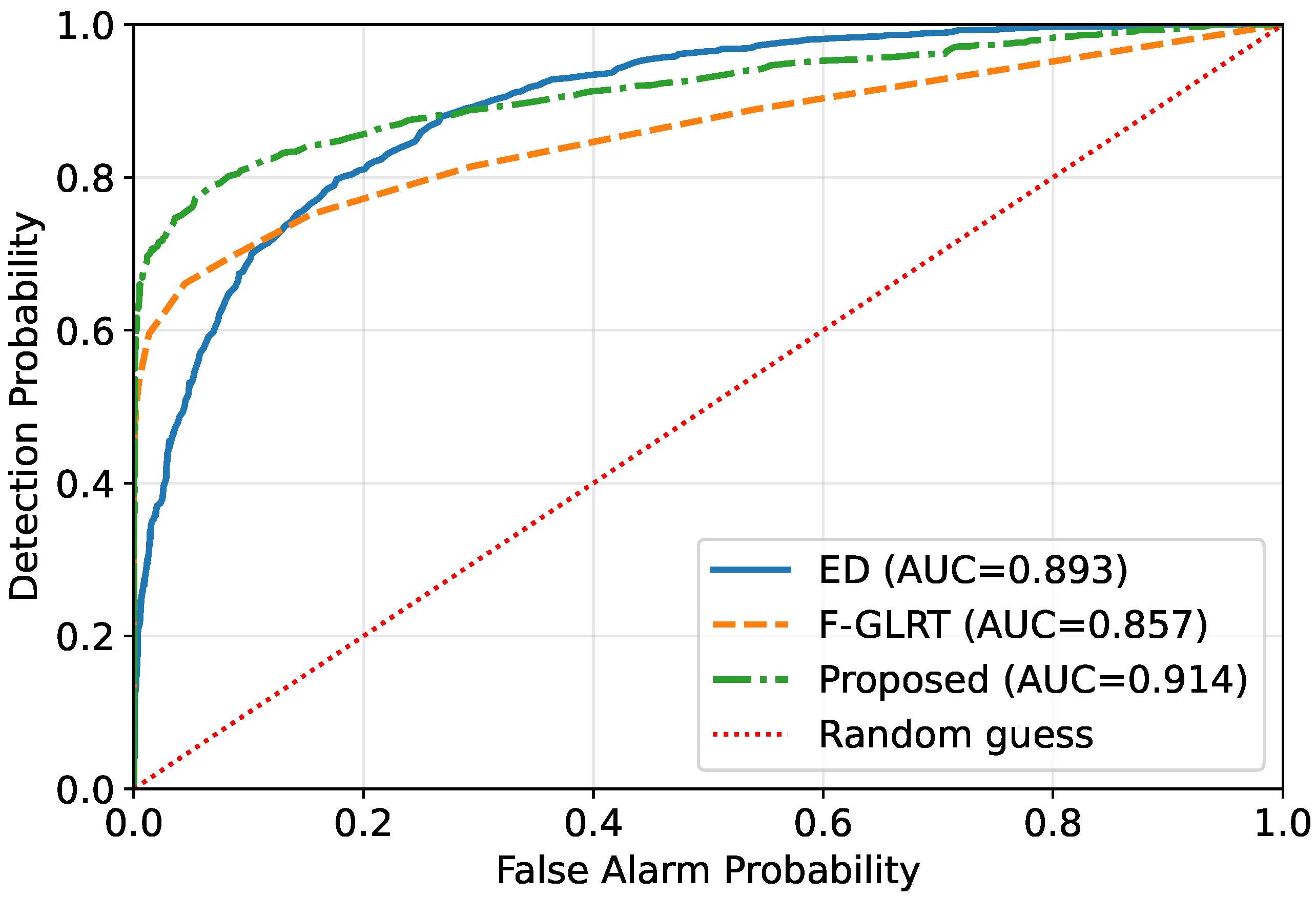
As shown in Figure 2, the proposed detector achieves the best overall ROC performance under matched environmental conditions at SNR = 14 dB. In particular, the proposed scheme attains the largest area under the curve (AUC = 0.914), indicating that the hierarchical Bayesian framework can more effectively exploit the weak-signal structure even when the propagation environment is correctly specified. By comparison, the conventional energy detector yields an AUC of 0.893, while the fixed-environment GLRT achieves an AUC of 0.857. This suggests that although the GLRT incorporates nominal channel information, its performance remains sensitive to the assumed template and does not fully benefit from the structured prior modeling introduced in the proposed method. The energy detector, on the other hand, relies only on overall energy accumulation and therefore lacks robustness in distinguishing weak target components from colored background noise.
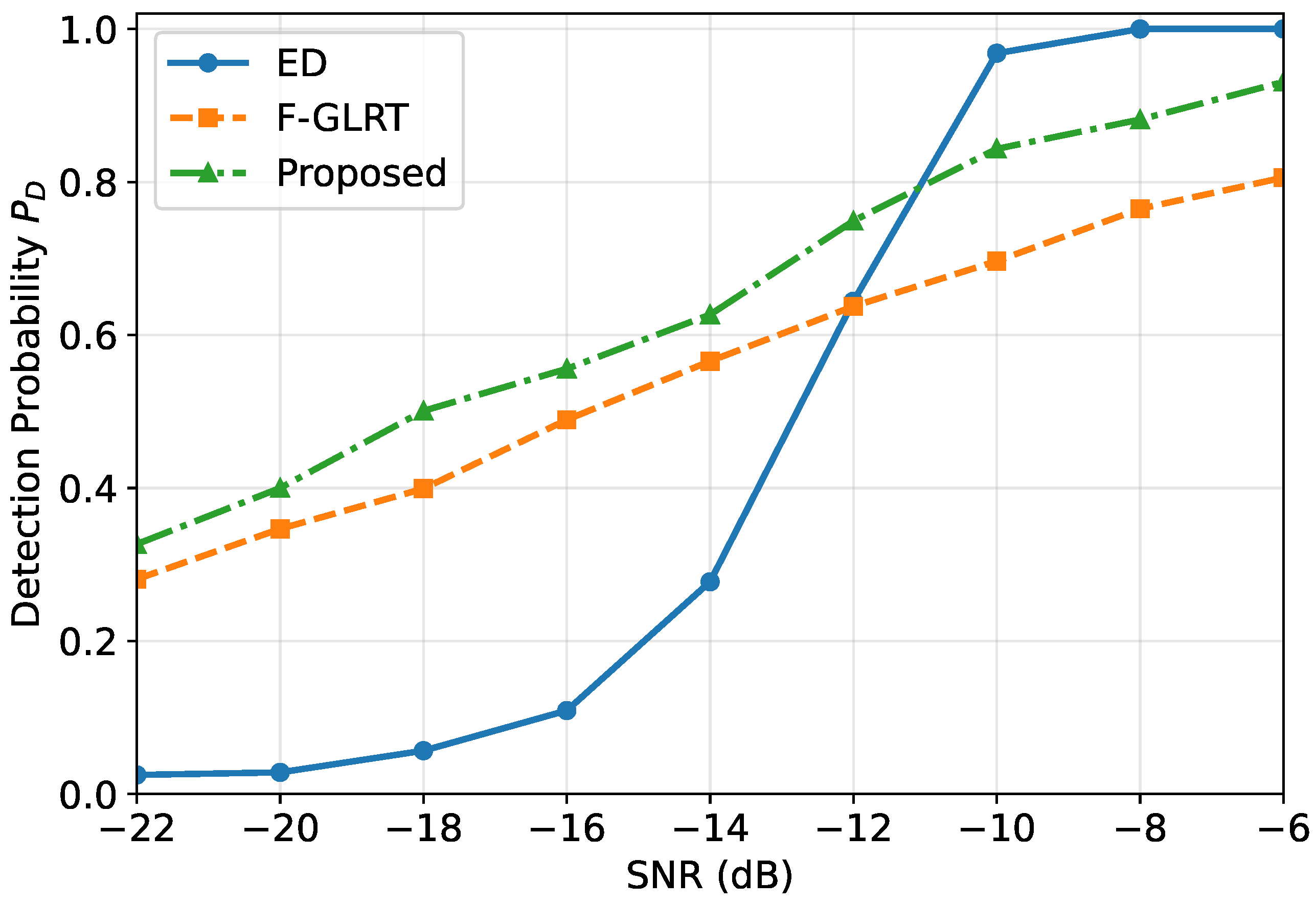
Figure 3 illustrates the detection probability of different detectors versus SNR under matched environmental conditions with a fixed false-alarm probability of P FA = 10 2 . It can be observed that the proposed detector achieves the highest detection probability throughout the low-to-moderate SNR region, demonstrating its clear advantage in weak-signal detection. In particular, when the SNR is below approximately 12 dB, the proposed method consistently outperforms both the conventional energy detector and the fixed-environment GLRT. This indicates that the hierarchical Bayesian framework can better exploit the structured spectral characteristics of weak underwater acoustic signals and thereby provide improved robustness in the challenging low-SNR regime. By comparison, the energy detector performs poorly in this region because it only relies on global energy accumulation and cannot effectively distinguish weak target components from colored background noise. The fixed-environment GLRT improves upon the energy detector by incorporating nominal propagation information, but its performance gain remains limited due to its dependence on a fixed template model. As the SNR further increases, the performance gap gradually narrows. In the relatively high-SNR regime, the energy detector also exhibits a rapid improvement because the target energy becomes sufficiently pronounced in the observation. Nevertheless, the proposed method still maintains consistently strong performance across the entire SNR range. This result suggests that the main strength of the proposed detector lies in enhancing robustness and sensitivity in the weak-signal regime, which is the primary operating condition considered in this work.
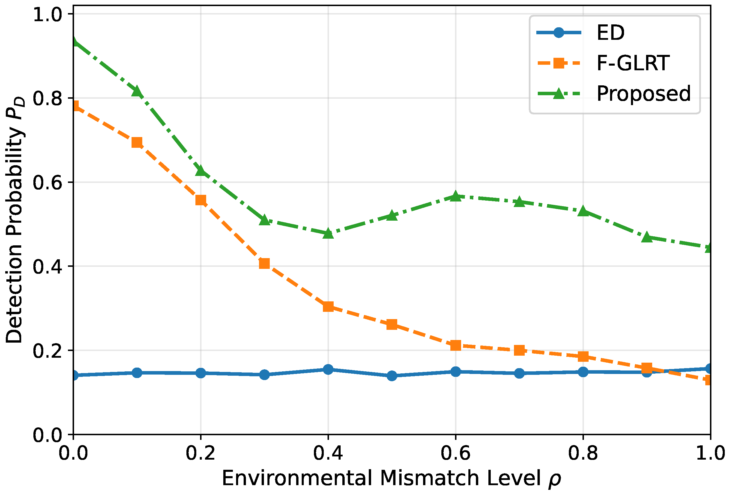
As shown in Figure 4, the detection performance of the fixed-environment GLRT degrades significantly as the environmental mismatch level increases. This result confirms that detectors relying on a single nominal propagation model are highly sensitive to mismatch in underwater acoustic channels. In contrast, the proposed detector consistently achieves the highest detection probability over the entire mismatch range and exhibits a much slower degradation trend, demonstrating its superior robustness against environmental uncertainty. The conventional energy detector maintains a relatively flat performance curve as the mismatch level increases, since it does not explicitly depend on the propagation model. However, its overall detection probability remains much lower than that of the proposed method because it does not exploit the structural characteristics of weak underwater signals. By comparison, the proposed method effectively mitigates the mismatch-induced degradation by incorporating environmental uncertainty into the detection process, thereby preserving a clear performance advantage under both mild and severe mismatch conditions.
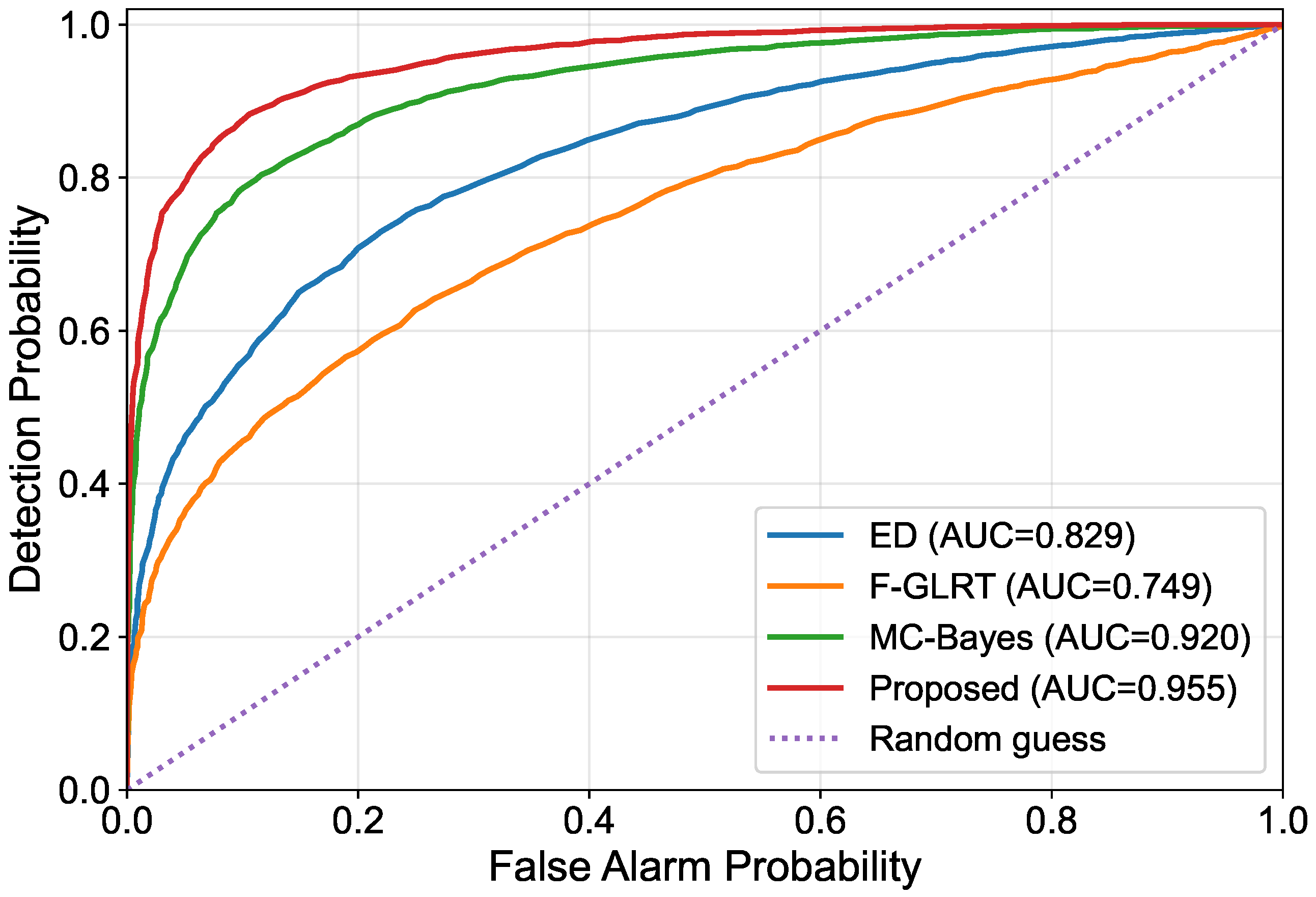
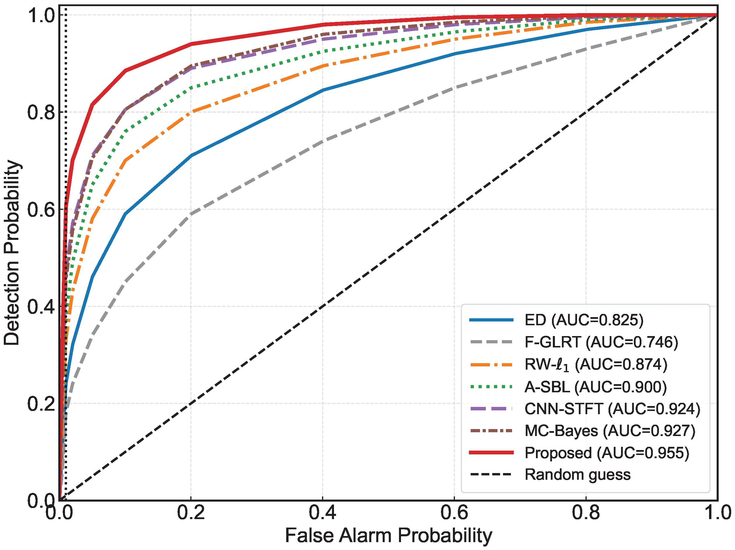
Figure 5 shows the ROC curves under severe environmental mismatch with ρ = 0.8 and SNR = 14 dB. To avoid relying only on weak or fixed-environment baselines, we additionally include an MC-Bayes baseline, which approximates environmental marginalization by averaging likelihood scores over sampled environmental states without performing the proposed variational posterior refinement. Therefore, it serves as a stronger Bayesian-style reference than the fixed-environment GLRT. It can be observed that the fixed-environment GLRT suffers a clear performance degradation under severe mismatch, confirming that a detector relying on a single nominal propagation template is vulnerable when the true underwater channel deviates from the assumed model. The MC-Bayes baseline significantly improves over F-GLRT by explicitly averaging over environmental uncertainty. Nevertheless, the proposed detector achieves the best overall ROC performance, with an AUC of 0.955, compared with 0.920 for MC-Bayes, 0.829 for ED, and 0.749 for F-GLRT. This result suggests that the proposed hierarchical variational inference framework provides an additional robustness advantage beyond direct environmental likelihood averaging in the considered controlled simulation setting.
To further address the concern regarding limited baseline comparison, we additionally include three stronger representative baselines in Figure 6: A-SBL, RW- 1 , and CNN-STFT. More specifically, A-SBL represents adaptive sparse Bayesian learning under the nominal propagation operator, RW- 1 represents reweighted sparse recovery for weak line-spectrum detection, and CNN-STFT represents a learning-based detector using the log-magnitude time–frequency representation. These additional baselines are evaluated under the same severe mismatch setting with ρ = 0.8 , SNR = 14 dB, and identical false-alarm calibration.
The results show that RW- 1 , A-SBL, and CNN-STFT achieve AUC values of 0.874, 0.900, and 0.924, respectively, outperforming ED and F-GLRT and thus providing more competitive references. MC-Bayes also achieves strong performance with an AUC of 0.927. Nevertheless, the proposed detector achieves the best overall ROC performance with an AUC of 0.955 and the highest detection probability at P FA = 10 2 . This demonstrates that the proposed framework remains advantageous even when compared with stronger sparse-recovery and learning-based baselines because it jointly exploits weak-signal sparsity and explicit environmental marginalization rather than relying on a fixed nominal propagation model or purely data-driven discrimination.
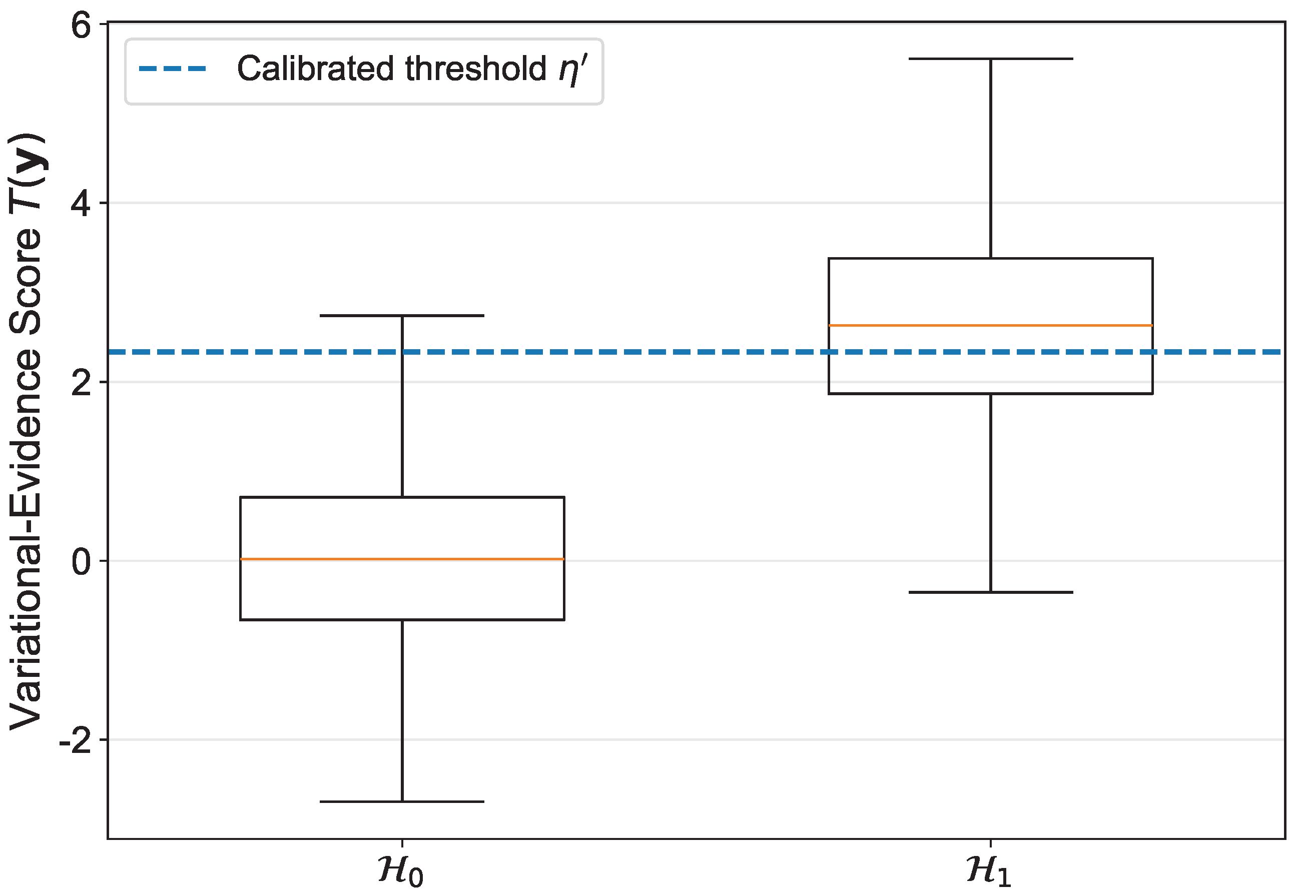
Although the proposed detection statistic is derived from the ELBO rather than from the exact marginal likelihood, it can still serve as a valid calibrated detection score if it provides statistical separation between signal-absent and signal-present observations. To examine this point, Figure 7 shows the distribution of the proposed variational-evidence score under H 0 and H 1 in the severe-mismatch case with ρ = 0.8 and SNR = 14 dB. The dashed line denotes the threshold calibrated from independent H 0 samples at P FA = 10 2 . It can be observed that most H 0 samples are concentrated below the calibrated threshold, while the H 1 scores are shifted to a significantly higher range. This empirical separation supports the use of the ELBO-based statistic as a practical score-based detector, although it is not claimed to be the exact Neyman–Pearson likelihood-ratio statistic.
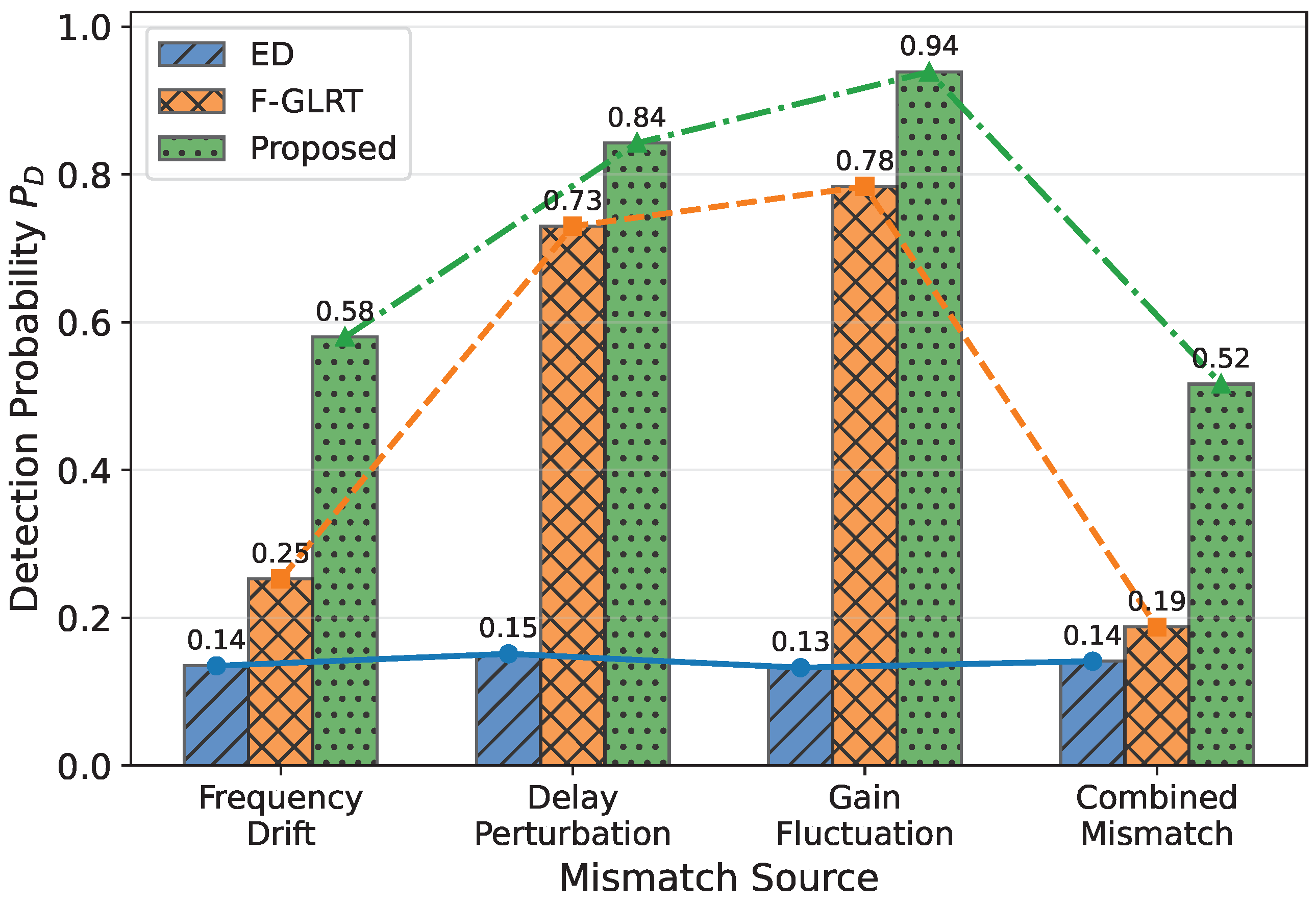
Figure 8 compares the detection performance of different methods under four representative uncertainty sources, including frequency drift, delay perturbation, gain fluctuation, and combined mismatch. It can be observed that the proposed detector consistently achieves the highest detection probability in all considered cases, demonstrating that its advantage is not limited to a single type of environmental or model uncertainty. For the conventional energy detector, the detection probability remains low and nearly unchanged across different uncertainty sources. This is because the energy detector does not explicitly exploit either the signal structure or the propagation model, and therefore cannot effectively distinguish weak target components from background noise. In contrast, the fixed-environment GLRT exhibits strong sensitivity to the type of mismatch. In particular, its performance degrades severely under frequency drift and combined mismatch, indicating that a detector built on a single nominal template can be highly vulnerable to spectral or structural deviations from the assumed model.
The proposed method maintains the best performance under all four cases and shows especially clear advantages under frequency drift and combined mismatch. This suggests that the proposed hierarchical Bayesian framework can effectively mitigate the impact of heterogeneous uncertainty sources by incorporating structured weak-signal priors together with environmental marginalization. Moreover, the combined mismatch case is the most challenging scenario for all compared methods, yet the proposed detector still preserves a substantial performance margin, further confirming its robustness in realistic underwater acoustic environments.
To assess the computational practicality of the proposed detector, we further demonstrate the average runtime per observation window in Table 2. All simulation experiments were conducted on the same desktop workstation under an identical software environment. The algorithms were implemented in Python 3.11 using NumPy and SciPy, and all reported simulations were executed on CPU without GPU acceleration. This setting ensures that the runtime and performance comparisons among different detectors are conducted under consistent hardware and software conditions. The runtime is measured after threshold calibration and averaged over independent Monte Carlo trials under the same simulation setting with N = 4096 and M = 701 . The observation-window duration is T obs = 1 s. As expected, ED has the lowest runtime because it only requires energy accumulation. F-GLRT is more expensive because it performs nominal-model fitting over the search grid. MC-Bayes further increases the computational cost because it approximates environmental marginalization by averaging likelihood scores over sampled environmental states. The proposed VB-EMD detector requires iterative variational posterior updates and is therefore slower than ED and F-GLRT. Nevertheless, its average runtime is 72.5 ms per 1 s observation window, which remains well below the observation duration in the considered setting. Moreover, the proposed method is faster than the MC-Bayes marginalization baseline while achieving better detection performance. These results indicate that the proposed detector is computationally feasible for offline or near-real-time processing in the present proof-of-concept simulation setting.
To further clarify the computational scalability, we analyze the complexity of the proposed VB-EMD detector with respect to the main problem dimensions. Let N t denote the number of time samples per receiver, N r denote the number of receivers or sensors, and N = N r N t denote the total observation dimension. Let M be the dictionary size, L p be the number of effective multipath components, d θ and d ξ be the dimensions of the target-related and environmental parameter vectors, respectively, and S be the number of sigma points used for quadrature. For the sigma-point rule used in this work, S typically scales as S = O ( d θ + d ξ ) . Let I denote the number of VB iterations. At each VB iteration, constructing the effective sensing matrices over all sigma points requires approximately O S N r N t M L p operations for the multipath forward model. After noise prewhitening or for structured noise covariance, the computation of the expected Gram matrix G ^ and correlation vector g ^ requires approximately O S N M 2 + S N M operations. The posterior update of q ( x ) involves solving an M × M linear system, whose direct cost is O ( M 3 ) . The updates of q ( α ) require only O ( M ) operations. The local Laplace updates of q ( θ ) and q ( ξ ) depend on the chosen numerical optimizer. If finite-difference Hessian evaluation is used, their cost scales with the number of local objective evaluations, which is approximately quadratic in d θ and d ξ . Since each objective evaluation involves the same forward-model and quadratic-form calculations, this term can be written as O ( d θ 2 + d ξ 2 ) C obj , where C obj denotes the cost of one local objective evaluation. Therefore, the overall complexity of the proposed detector is approximately O I S N r N t M L p + S N M 2 + M 3 + ( d θ 2 + d ξ 2 ) C obj .
For larger sensing systems, several implementation strategies can improve scalability. First, the effective dictionary can be restricted to a physically plausible frequency band or updated using an active-set sparse Bayesian strategy, thereby reducing M. Second, the sigma-point evaluations are independent and can be parallelized across environmental samples and receiver channels. Third, when R n has Toeplitz, block-diagonal, or approximately diagonal structure after prewhitening, matrix-vector products involving R n 1 can be implemented efficiently without forming a dense inverse. Finally, iterative linear solvers or low-rank covariance approximations can be used to avoid the full O ( M 3 ) cost when M becomes large. These observations indicate that the proposed detector is suitable for offline or near-real-time processing under the current problem size, while larger multi-receiver systems require structured linear algebra and dictionary-pruning strategies for scalable deployment.

5.3. Ablation Experiments

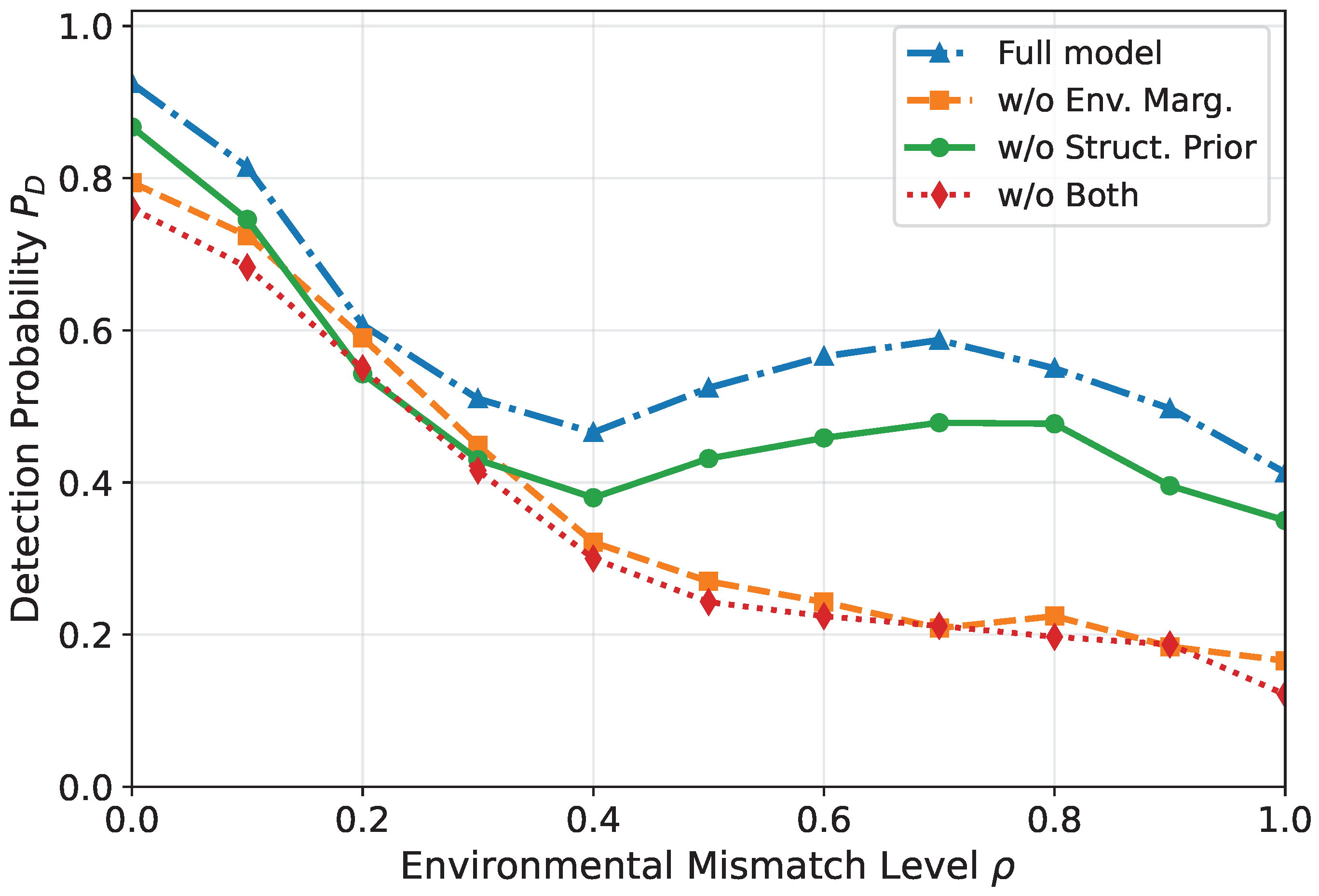
To directly support the contribution of each modeling component, we conduct an ablation study by comparing the full model with three degraded variants. The full model uses both environmental marginalization and the structured weak-signal prior. The “w/o Env. Marg.” variant fixes the environmental variable at the nominal condition, i.e., it removes the marginalization over ξ while retaining the structured prior. The “w/o Struct. Prior” variant retains environmental marginalization but replaces the sparse hierarchical prior with a non-sparse Gaussian prior. The “w/o Both” variant removes both environmental marginalization and the structured prior. All variants are evaluated using the same data generation, threshold calibration, and testing protocol.
Figure 9 presents the ablation study of the proposed detector under different environmental mismatch levels. Four variants are considered, including the full model, the version without environmental marginalization, the version without the structural prior, and the version without both components. It can be observed that the full model consistently achieves the highest detection probability across the entire mismatch range, confirming the effectiveness of jointly incorporating environmental marginalization and structured weak-signal modeling. A clear performance degradation is observed when environmental marginalization is removed. In particular, the w/o Env. Marg. curve drops rapidly as the mismatch level increases and remains close to the w/o Both case in the moderate-to-severe mismatch region. This indicates that environmental marginalization is the main source of robustness against propagation uncertainty. Without this component, the detector becomes much more sensitive to model mismatch and loses a substantial portion of its detection capability. On the other hand, the w/o Struct. Prior variant still performs noticeably better than the w/o Env. Marg. and w/o Both variants, which shows that environmental marginalization alone already provides a significant robustness gain. Nevertheless, its performance remains consistently below that of the full model, demonstrating that the structural prior offers an additional performance improvement by enhancing sensitivity to weak tonal components. Therefore, the ablation results verify that the proposed detector benefits from two complementary mechanisms: Environmental marginalization provides the dominant robustness improvement, while the structural prior further strengthens weak-signal discrimination.

6. Conclusions

This paper investigated weak underwater acoustic signal detection under environmental mismatch and developed a hierarchical Bayesian detector that explicitly incorporates uncertain propagation conditions into the detection process. Unlike conventional fixed-environment detectors that rely on a nominal propagation model, the proposed framework treats the environmental state as a latent random variable and combines environmental uncertainty modeling with structured weak-signal priors within a unified Bayesian hypothesis-testing formulation. Based on this model, a variational Bayesian approximation was developed to obtain a tractable evidence-based detection statistic for practical implementation.
Simulation results demonstrated that the proposed detector achieves consistently strong performance under both matched and mismatched underwater conditions. In particular, the method showed clear advantages in the low-SNR regime, where weak target components are easily masked by colored background noise and propagation uncertainty can cause severe degradation for nominal-model-based detectors. The results further showed that, as the environmental mismatch level increases, the proposed detector degrades much more slowly than the fixed-environment GLRT, confirming the robustness benefit of explicit environmental marginalization. Moreover, the ablation study revealed that environmental marginalization is the dominant source of robustness improvement, while the structural weak-signal prior provides an additional gain in weak-signal discrimination.
The limitation of the proposed method is that its current validation is based on controlled synthetic simulations rather than measured at-sea data. Therefore, the reported results should be considered as proof-of-concept evidence under prescribed environmental uncertainty models rather than as complete field validation. The method may fail or degrade when the true propagation condition lies outside the assumed environmental prior, when the noise covariance is strongly mismatched or dominated by non-Gaussian impulsive interference, or when the target signature does not match the assumed weak narrowband/sparse spectral structure. In these cases, the variational posterior may assign high evidence to an incorrect environmental or signal configuration, leading to degraded detection performance.
Future work will further validate the proposed framework using measured underwater acoustic datasets with reliable signal-present/signal-absent labels, synchronized environmental measurements, and realistic low-SNR target observations. Such validation will be important for assessing the field-level robustness of the proposed detector beyond the controlled effective propagation models considered in this paper.

Author Contributions

Conceptualization, Y.W. and J.L.; methodology, Y.W.; software, Y.W.; validation, Y.W. and J.L.; formal analysis, Y.W.; investigation, Y.W.; resources, J.L.; data curation, J.L.; writing—original draft preparation, Y.W. and J.L.; writing—review and editing, Y.W. and J.L.; visualization, Y.W. and J.L.; supervision, J.L.; project administration, J.L.; funding acquisition, J.L. All authors have read and agreed to the published version of the manuscript.

Funding

This research received no external funding.

Institutional Review Board Statement

Not applicable.

Informed Consent Statement

Not applicable.

Data Availability Statement

The data presented in this study are available on request from the corresponding author due to privacy and institutional restrictions.

Conflicts of Interest

The authors declare no conflicts of interest.

Appendix A. Convergence Analysis of the Proposed VB-EMD Algorithm

This appendix discusses the convergence property of the proposed VB-EMD algorithm. Since the exact marginal likelihood is analytically intractable, the algorithm optimizes the quadrature-approximated variational evidence lower bound introduced in Section 4.4. Let L ˜ q ( x ) , q ( α ) , q ( θ ) , q ( ξ ) denote the numerically evaluated ELBO under the adopted mean-field factorization q ( x , α , θ , ξ ) = q ( x ) q ( α ) q ( θ ) q ( ξ ) . Here, the notation L ˜ is used to emphasize that the expectations over θ and ξ are evaluated using the deterministic sigma-point approximation described in Section 4.4. For fixed q ( θ ) , q ( ξ ) , and q ( α ) , the update of q ( x ) follows the standard coordinate-wise variational rule:
ln q ( x ) = E q ( α ) q ( θ ) q ( ξ ) ln p ( y , x , α , θ , ξ ) + const .
Therefore, the update of q ( x ) maximizes L ˜ with respect to q ( x ) while keeping the other variational factors fixed. Similarly, the update of q ( α ) is obtained from the conjugate Gamma posterior and maximizes L ˜ with respect to q ( α ) under the adopted mean-field factorization. Hence, these two updates are non-decreasing steps of the computed ELBO. It should be noted that the convergence result discussed here refers to the numerically evaluated quadrature-approximated ELBO sequence, rather than to the exact marginal likelihood or to a globally optimal posterior solution.
The updates of q ( θ ) and q ( ξ ) are different, because the propagation operator is nonlinear in these variables and closed-form coordinate-wise VB updates are unavailable. In the proposed algorithm, these two posterior factors are updated by local Laplace approximations. Specifically, their means are obtained from local maximization of J θ ( θ ) and J ξ ( ξ ) , and their covariance matrices are computed from the corresponding regularized local curvature matrices. To ensure a non-decreasing variational objective, the local Newton or quasi-Newton step is implemented with a damping strategy. If a candidate update decreases the computed ELBO, the step size is reduced; if no acceptable increase is found, the previous variational factor is retained. Therefore, the accepted Laplace update satisfies
L ˜ ( i + 1 ) L ˜ ( i ) .
Combining the above block updates, the sequence { L ˜ ( i ) } i = 1 generated by the proposed VB-EMD algorithm is monotonically non-decreasing. Moreover, under the assumed finite noise covariance, proper priors, finite observation energy, finite quadrature points, and positive-definite posterior covariance matrices enforced by diagonal loading when necessary, the computed ELBO is finite and upper bounded. Consequently, the monotone convergence theorem implies that
lim i L ˜ ( i ) = L ˜ ,
where L ˜ is a finite limit.

References

  1. Hummel, H.I.; van der Mei, R.; Bhulai, S. A survey on machine learning in ship radiated noise. Ocean Eng. 2024, 298, 117252. [Google Scholar] [CrossRef]
  2. Chen, R.; Schmidt, H. Model-based convolutional neural network approach to underwater source-range estimation. J. Acoust. Soc. Am. 2021, 149, 405–420. [Google Scholar] [CrossRef] [PubMed]
  3. Zhang, D.; Gao, L.; Sun, D.; Teng, T. Soft-decision detection of weak tonals for passive sonar using track-before-detect method. Appl. Acoust. 2022, 188, 108549. [Google Scholar] [CrossRef]
  4. Chen, Y.; Wang, Y.; Wang, Z.; Han, Z. Angular-Distance Based Channel Estimation for Holographic MIMO. IEEE J. Sel. Areas Commun. 2024, 42, 1684–1702. [Google Scholar] [CrossRef]
  5. Chen, Y.; Guo, X.; Zhou, G.; Jin, S.; Ng, D.W.K.; Wang, Z. Unified Far-Field and Near-Field in Holographic MIMO: A Wavenumber-Domain Perspective. IEEE Commun. Mag. 2025, 63, 30–36. [Google Scholar] [CrossRef]
  6. Zhang, L.; Piao, S.; Guo, J.; Wang, X. Multi-frame coherent track-before-detect method for weak tones in passive sonar. Signal Process. 2024, 220, 109437. [Google Scholar] [CrossRef]
  7. Zhang, L.; Piao, S.; Guo, J.; Wang, X. Variable frequency-based multi-frame coherent track-before-detect method for weak tones in passive sonar. J. Acoust. Soc. Am. 2025, 158, 923–945. [Google Scholar] [CrossRef]
  8. Ju, D.; Chi, C.; Li, Z.; Li, Y.; Zhang, C.; Huang, H. Deep-learning-based line enhancer for passive sonar systems. IET Radar Sonar Navig. 2022, 16, 589–601. [Google Scholar] [CrossRef]
  9. Dong, H.; Ma, S.; Suo, J.; Zhu, Z. Matched Stochastic Resonance Enhanced Underwater Passive Weak Signal Detection under Non-Gaussian Impulsive Background Noise. Sensors 2024, 24, 2943. [Google Scholar] [CrossRef]
  10. Shin, M.; Hong, W.; Lee, K.; Choo, Y. Frequency Analysis of Acoustic Data Using Multiple-Measurement Sparse Bayesian Learning. Sensors 2021, 21, 5827. [Google Scholar] [CrossRef]
  11. Shin, M.; Hong, W.; Lee, K.; Choo, Y. Passive Sonar Target Identification Using Multiple-Measurement Sparse Bayesian Learning. Sensors 2022, 22, 8511. [Google Scholar] [CrossRef] [PubMed]
  12. Ko, S.; Shin, M.; Kim, G.; Choo, Y. System-Informed Neural Network for Frequency Detection. IEEE Signal Process. Lett. 2024, 31, 2980–2984. [Google Scholar] [CrossRef]
  13. Ge, F.X.; Bai, Y.; Li, M.; Zhu, G.; Yin, J. Label distribution-guided transfer learning for underwater source localization. J. Acoust. Soc. Am. 2022, 151, 4140. [Google Scholar] [CrossRef]
  14. Hu, Y.; Sun, X.; He, L.; Huang, H. A generalized network based on multi-scale densely connection and residual attention for sound source localization and detection. J. Acoust. Soc. Am. 2022, 151, 1754–1768. [Google Scholar] [CrossRef] [PubMed]
  15. Cao, Y.; Shi, W.; Sun, L.; Fu, X. Frequency Diversity Based Underwater Acoustic Passive Localization. IEEE Internet Things J. 2022, 9, 12641–12655. [Google Scholar] [CrossRef]
  16. Kim, J. Surface Target Tracking Using Towed Array Sonars with Direct and Bottom Bounce Underwater Sound Signals. IEEE Trans. Signal Inf. Process. Netw. 2022, 8, 997–1007. [Google Scholar] [CrossRef]
  17. He, Q.; Qu, C.; Zuo, W. Planning Waste-to-Energy-Coupled AI Data Centers Through Grade-Matched Cooling and Corridor Screening. Thermo 2026, 6, 28. [Google Scholar] [CrossRef]
  18. He, Q.; Shan, R.; Qu, C.; Tang, Y.; Zou, Y. The Material Blind Spot of the AI Revolution: Rare-Earth Dependencies Undermine Sustainable Digital Future. Available online: https://ssrn.com/abstract=6232318 (accessed on 30 January 2026).
  19. He, J.; Zhang, B.; Liu, P.; Li, X.; Wang, L.; Tang, R. Effective underwater acoustic target passive localization of using a multi-task learning model with attention mechanism: Analysis and comparison under real sea trial datasets. Appl. Ocean Res. 2024, 150, 104072. [Google Scholar] [CrossRef]
  20. Grumiaux, P.A.; Kitić, S.; Girin, L.; Guérin, A. A survey of sound source localization with deep learning methods. J. Acoust. Soc. Am. 2022, 152, 107–151. [Google Scholar] [CrossRef] [PubMed]
  21. Lv, H.; Li, C.; Dai, J.; Zhang, Y.; Fan, Z.; Tan, Y.; Wang, D.; Xie, B. Lightweight Framework for Underground Pipeline Recognition and Spatial Localization Based on Multiview 2-D GPR Images. IEEE Trans. Geosci. Remote Sens. 2025, 63, 5110115. [Google Scholar] [CrossRef]
  22. Wang, D.; Lv, H.; Zhang, Y.; Fan, Z.; Ni, Y.; Lv, S.; Shen, P.; Tang, F.; Wu, H. Monitoring and Detection Technologies and AI-Powered Development Toward Transparent Roads. Engineering, 2025; in press. [CrossRef]
  23. Yu, Y.; Wang, C.; Wang, W.; Lu, K.; Chen, Z.; Zhao, D.; Ju, B.F.; Zhou, S. Determination of elastic constants in unidirectional CFRP laminates using neural networks and laser ultrasonic bulk waves. Compos. Part A Appl. Sci. Manuf. 2026, 207, 109827. [Google Scholar] [CrossRef]
  24. Ren, S.J.; Deng, J.; Wang, J.R.; Wang, C.P.; Xiao, Y.; Kang, F.R.; Li, H.-J.; Dou, L.H. Porosity inversion and determination in gob unconsolidated materials based on acoustic signal response. Fuel 2026, 426, 139614. [Google Scholar] [CrossRef]
  25. Zhang, B.; Jin, R.; Jiang, L.; Yang, L.; Zhang, T. Robust Sparse Bayesian Learning Source Localization in an Uncertain Shallow-Water Waveguide. Electronics 2024, 13, 4789. [Google Scholar] [CrossRef]
  26. Wang, Q.; Yu, H.; Chen, Y.; Dong, C.; Li, J.; Ji, F. Noise-free fast sparse Bayesian learning method for robust multi-frequency underwater matched-field acoustic source localization. Appl. Acoust. 2025, 228, 110356. [Google Scholar] [CrossRef]
  27. Wang, J.; Zhang, L.; Hu, B.; Wu, D.; Hu, X. Sparse Bayesian learning based on spatio-temporal structure-aware for matched field processing. J. Acoust. Soc. Am. 2024, 155, 328–342. [Google Scholar] [CrossRef]
  28. Miao, H.; Li, L.; Zhang, Y.; Cao, R.; Liu, M.; Zhang, B. Correction physics-informed neural network-aided matched field processing technique for underwater passive source range estimation. J. Acoust. Soc. Am. 2025, 158, 235–258. [Google Scholar] [CrossRef]
  29. Kari, D.; Zhuang, Y.; Singer, A.C. Mismatch-Robust Underwater Acoustic Localization Using A Differentiable Modular Forward Model. In Proceedings of the 2025 59th Annual Conference on Information Sciences and Systems (CISS), Baltimore, MD, USA, 19–21 March 2025. [Google Scholar] [CrossRef]
  30. Li, J.; Li, H.; Guo, X.; Ma, L. Broadband source localization using near-surface vertical array in deep ocean based on sparse Bayesian learning. Acta Acust. 2025, 50, 703–717. [Google Scholar] [CrossRef]
  31. Liu, X.; Wang, C.; Chen, C.; Pan, Z.; Xiao, W. Recent advances in hierarchical porous materials for CO2 capture and utilization. Coord. Chem. Rev. 2025, 544, 216927. [Google Scholar] [CrossRef]
  32. Wang, S.; Liu, M.; Li, D. Bayesian Learning-Based Clustered-Sparse Channel Estimation for Time-Varying Underwater Acoustic OFDM Communication. Sensors 2021, 21, 4889. [Google Scholar] [CrossRef]
  33. Jia, S.; Zou, S.; Zhang, X.; Tian, D.; Da, L. Multi-block Sparse Bayesian learning channel estimation for OFDM underwater acoustic communication based on fractional Fourier transform. Appl. Acoust. 2022, 192, 108721. [Google Scholar] [CrossRef]
  34. Feng, X.; Wang, J.; Sun, H.; Qi, J.; Qasem, Z.A.H.; Cui, Y. Channel estimation for underwater acoustic OFDM communications via temporal sparse Bayesian learning. Signal Process. 2023, 207, 108951. [Google Scholar] [CrossRef]
  35. Yin, J.; Zhu, G.; Han, X.; Guo, L.; Li, L.; Ge, W. Temporal Correlation and Message-Passing-Based Sparse Bayesian Learning Channel Estimation for Underwater Acoustic Communications. IEEE J. Ocean. Eng. 2024, 49, 522–541. [Google Scholar] [CrossRef]
  36. Zou, S.; Jia, S.; Zhang, X.; Liu, B. A fast temporal multiple sparse Bayesian learning-based channel estimation method for time-varying underwater acoustic OFDM systems. Front. Commun. Netw. 2024, 5, 1465902. [Google Scholar] [CrossRef]
  37. Guo, J.; Guo, T.; Li, M.; Wu, T.; Lin, H. Underwater-Acoustic-OFDM Channel Estimation Based on Deep Learning and Data Augmentation. Electronics 2024, 13, 689. [Google Scholar] [CrossRef]
  38. Wu, X.; Wang, H.; Zhang, Y.; Zou, B.; Hong, H. A Tutorial-Generating Method for Autonomous Online Learning. IEEE Trans. Learn. Technol. 2024, 17, 1532–1541. [Google Scholar] [CrossRef] [PubMed]
  39. Wu, X.; Zhang, Y.T.; Lai, K.W.; Yang, M.Z.; Yang, G.L.; Wang, H.H. A Novel Centralized Federated Deep Fuzzy Neural Network with Multi-objectives Neural Architecture Search for Epistatic Detection. IEEE Trans. Fuzzy Syst. 2025, 33, 94–107. [Google Scholar] [CrossRef]
  40. Zhou, H.; Luo, X.; Chen, L. The weak modulation line spectrum enhancement and detection method for ship radiated noise in the absence of prior information. Appl. Acoust. 2024, 226, 110211. [Google Scholar] [CrossRef]
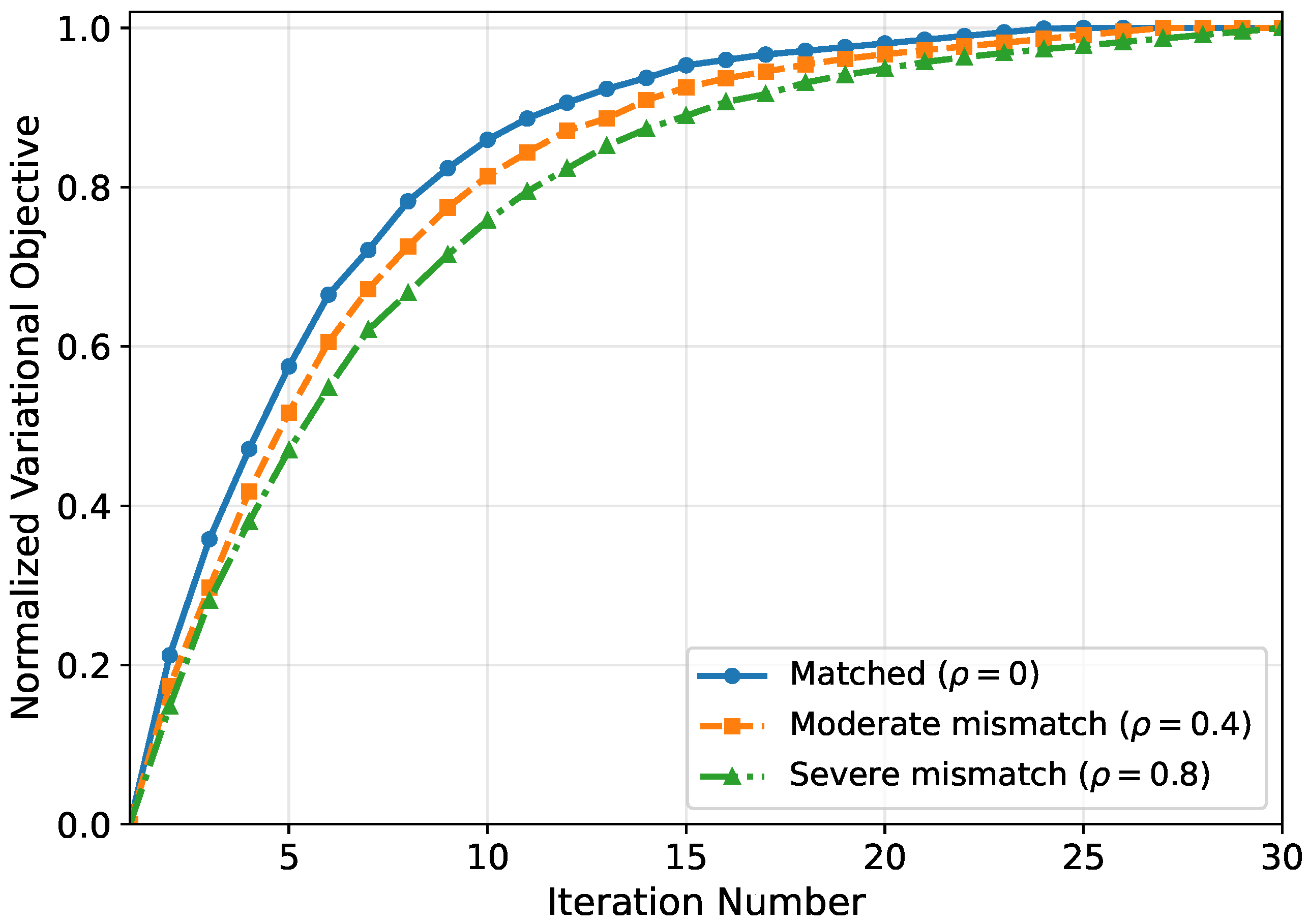
Figure 1. Convergence behavior of the proposed iterative detector under different environmental mismatch levels.
Electronics 15 02345 g001
Figure 2. ROC curves of different detectors under matched environmental conditions at SNR = 14 dB.
Electronics 15 02345 g002
Figure 3. Detection probability versus SNR under matched environmental conditions with P FA = 10 2 .
Electronics 15 02345 g003
Figure 4. Detection probability versus environmental mismatch level under SNR = 14 dB and P FA = 10 2 .
Electronics 15 02345 g004
Figure 5. ROC comparison under severe environmental mismatch with ρ = 0.8 and SNR = 14 dB.
Electronics 15 02345 g005
Figure 6. ROC comparison with stronger contemporary baselines under severe environmental mismatch with ρ = 0.8 and SNR = 14 dB.
Electronics 15 02345 g006
Figure 7. Distribution of the proposed variational-evidence score under H 0 and H 1 under severe environmental mismatch with ρ = 0.8 and SNR = 14 dB. The orange line inside each box denotes the median of the corresponding variational-evidence score distribution.
Electronics 15 02345 g007
Figure 8. Detection performance under different uncertainty sources at SNR = 14 dB and P FA = 10 2 .
Electronics 15 02345 g008
Figure 9. Ablation study under environmental mismatch with SNR = 14 dB and P FA = 10 2 .
Electronics 15 02345 g009
Table 1. Empirical threshold calibration and ablation fairness under severe environmental mismatch with ρ = 0.8 and SNR = 14 dB.
CategoryMethodTarget P FA Empirical P FA Empirical P D
Main detectorED 10 2 0.00900.2403
Main detectorF-GLRT 10 2 0.00830.1820
Main detectorMC-Bayes 10 2 0.00830.4553
Main detectorProposed 10 2 0.01150.6045
AblationFull model 10 2 0.01010.5800
Ablationw/o Env. Marg. 10 2 0.00980.2200
Ablationw/o Struct. Prior 10 2 0.01040.4600
Ablationw/o Both 10 2 0.00990.2000
Table 2. Average runtime comparison per observation window under the simulation setting with N = 4096 and M = 701 . The observation window duration is T obs = 1 s.
MethodAverage Iterations/SamplesRuntime per FrameRelative Runtime
ED0.24 ms1.0×
F-GLRTgrid search18.6 ms77.5×
MC-Bayes100 env. samples96.8 ms403.3×
Proposed VB-EMD18.4 iterations72.5 ms302.1×
Disclaimer/Publisher’s Note: The statements, opinions and data contained in all publications are solely those of the individual author(s) and contributor(s) and not of MDPI and/or the editor(s). MDPI and/or the editor(s) disclaim responsibility for any injury to people or property resulting from any ideas, methods, instructions or products referred to in the content.