Figure 1.
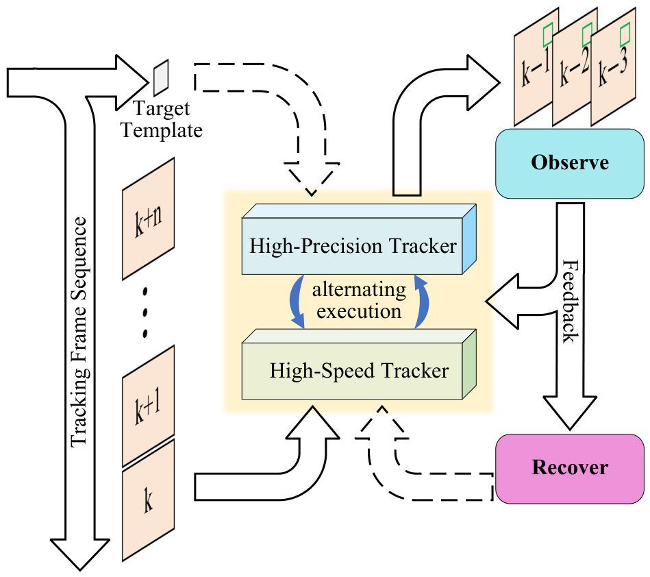
The framework of HCLT. By alternating between two trackers to complete the tracking process, it enables dynamic adjustment of computational load. Additionally, an observation-feedback-recovery channel is designed to further enhance the robustness of HCLT in real-world tracking tasks. Alternating execution is the main working mode in the tracking process, while Observe and Recover are external methods. Solid arrows denote the main task loop, and dashed arrows denote condition-triggered branch tasks.
Figure 1.
The framework of HCLT. By alternating between two trackers to complete the tracking process, it enables dynamic adjustment of computational load. Additionally, an observation-feedback-recovery channel is designed to further enhance the robustness of HCLT in real-world tracking tasks. Alternating execution is the main working mode in the tracking process, while Observe and Recover are external methods. Solid arrows denote the main task loop, and dashed arrows denote condition-triggered branch tasks.
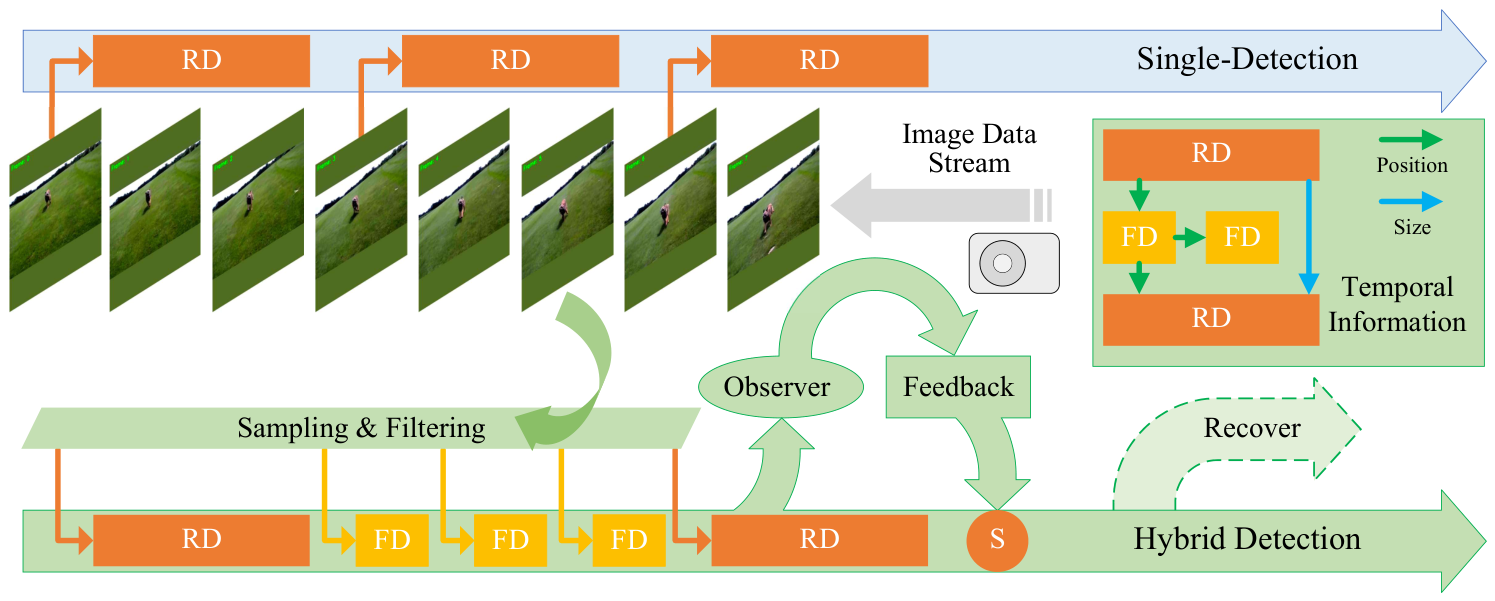
Figure 2.
HCLT’s framework, along with its comparison against single-detection tracking approaches, demonstrates a significant improvement in processing efficiency. Within the same time interval, HCLT is capable of handling a markedly greater number of frames. Blue indicates the single-detection working mode, and green indicates HCLT’s hybrid-detection working mode. The dashed Recover arrow indicates that the recovery process is used only when the target is judged to be lost.
Figure 2.
HCLT’s framework, along with its comparison against single-detection tracking approaches, demonstrates a significant improvement in processing efficiency. Within the same time interval, HCLT is capable of handling a markedly greater number of frames. Blue indicates the single-detection working mode, and green indicates HCLT’s hybrid-detection working mode. The dashed Recover arrow indicates that the recovery process is used only when the target is judged to be lost.
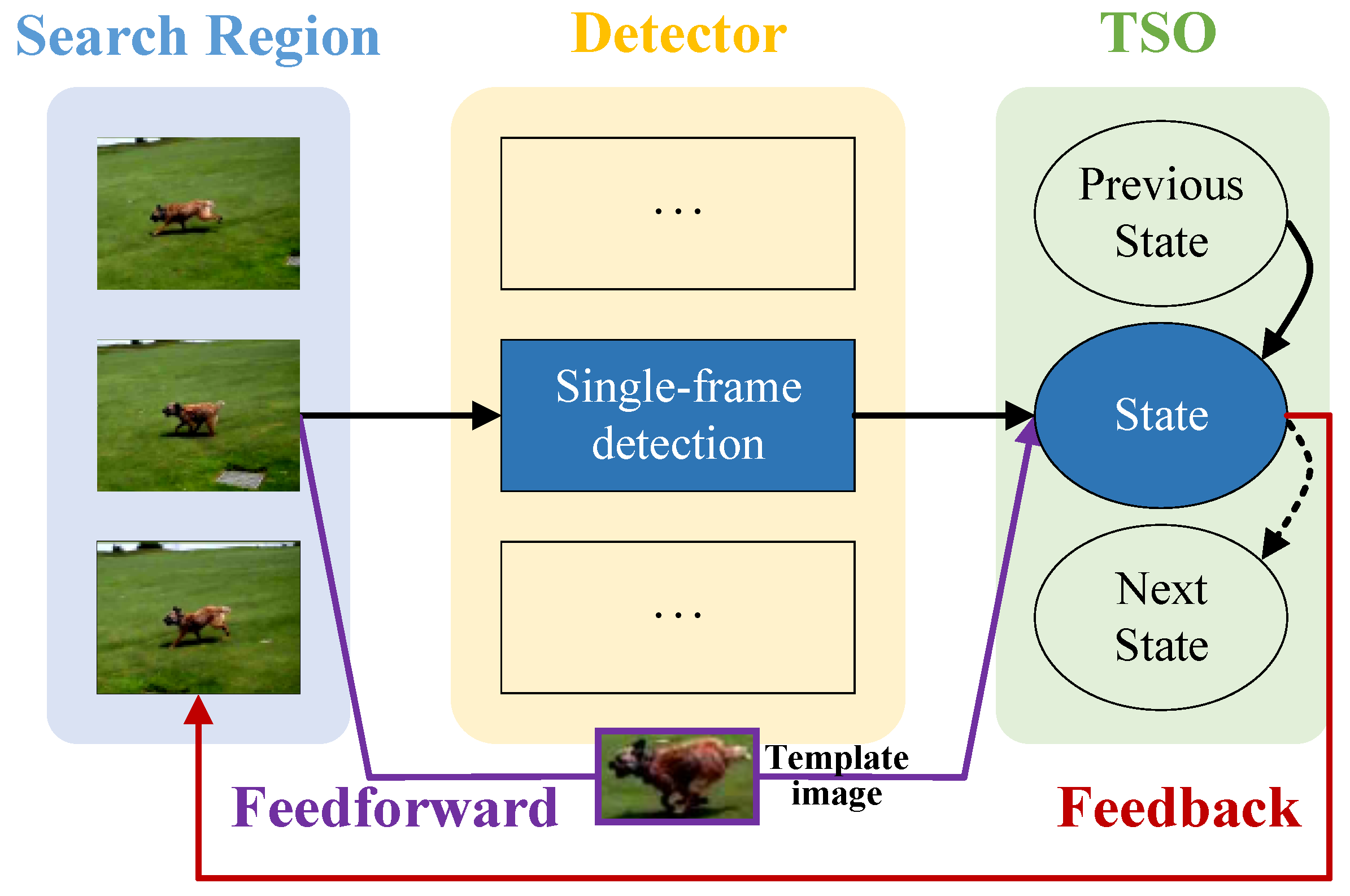
Figure 3.
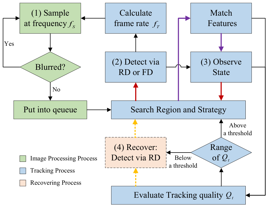
The workflow of HCLT mainly consists of four steps and can run across three distinct processes to enhance the tracking of real-time performance. Red arrows indicate the feedback process, and purple arrows indicate the feedforward process.
Figure 3.
The workflow of HCLT mainly consists of four steps and can run across three distinct processes to enhance the tracking of real-time performance. Red arrows indicate the feedback process, and purple arrows indicate the feedforward process.
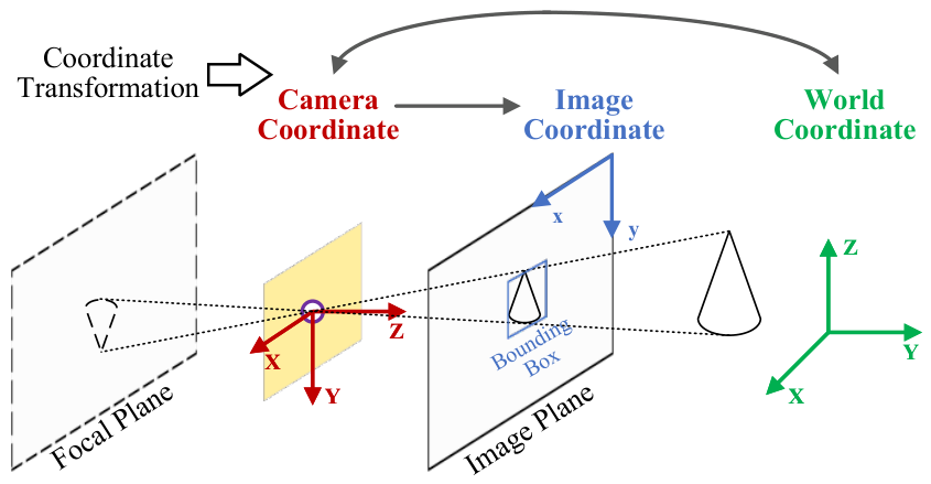
Figure 4.
Coordinate transformation and image-plane projection under camera motion. Camera motion may change the projected position of the target in the image plane and affect tracking; therefore, TSO considers such projection variations. Solid lines denote the coordinate axes, image plane, and target projection, while dashed lines indicate auxiliary projection rays and reference planes.
Figure 4.
Coordinate transformation and image-plane projection under camera motion. Camera motion may change the projected position of the target in the image plane and affect tracking; therefore, TSO considers such projection variations. Solid lines denote the coordinate axes, image plane, and target projection, while dashed lines indicate auxiliary projection rays and reference planes.
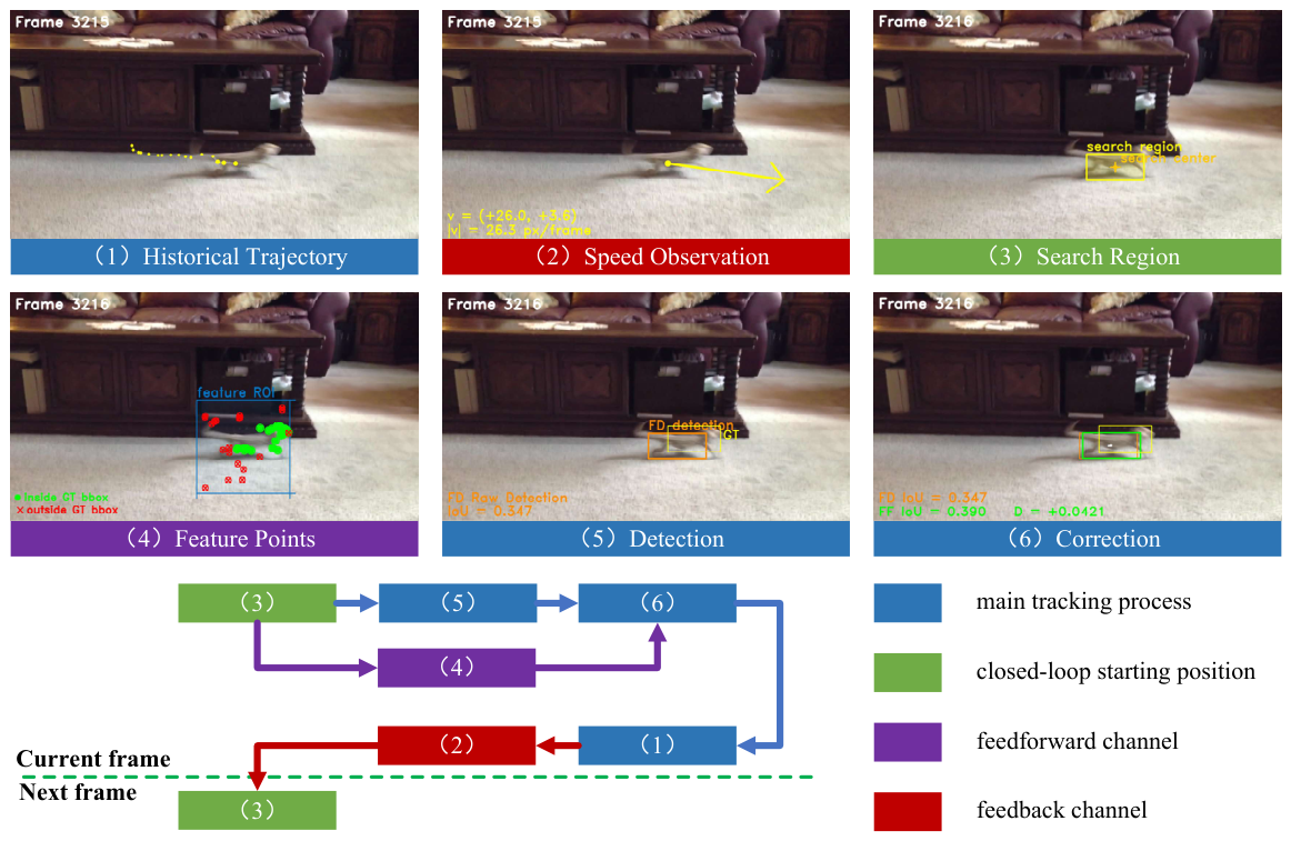
Figure 5.
The feedforward channel operates only on the current frame, while the feedback channel acts on the next frame. Spatial information adjusts the current state through the feedforward channel, and the current state acts on the search region of the next frame via the feedback channel. Red arrows indicate the feedback process, and purple arrows indicate the feedforward process.
Figure 5.
The feedforward channel operates only on the current frame, while the feedback channel acts on the next frame. Spatial information adjusts the current state through the feedforward channel, and the current state acts on the search region of the next frame via the feedback channel. Red arrows indicate the feedback process, and purple arrows indicate the feedforward process.
Figure 6.
Visualization of intermediate results during the tracking process. Incorporating velocity observations and feature points can enhance the accuracy and stability of tracking.
Figure 6.
Visualization of intermediate results during the tracking process. Incorporating velocity observations and feature points can enhance the accuracy and stability of tracking.
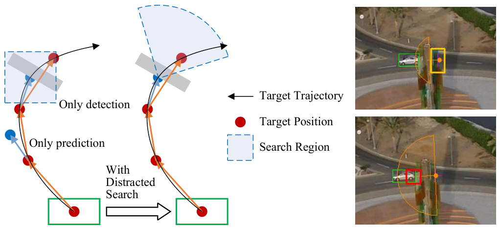
Figure 7.
Distracted search alters the traditional search strategy by utilizing velocity information to derive a new search region after tracking failure, thereby enabling tracking recovery. Blue dots denote incorrect target predictions, and red dots denote the true target positions.
Figure 7.
Distracted search alters the traditional search strategy by utilizing velocity information to derive a new search region after tracking failure, thereby enabling tracking recovery. Blue dots denote incorrect target predictions, and red dots denote the true target positions.
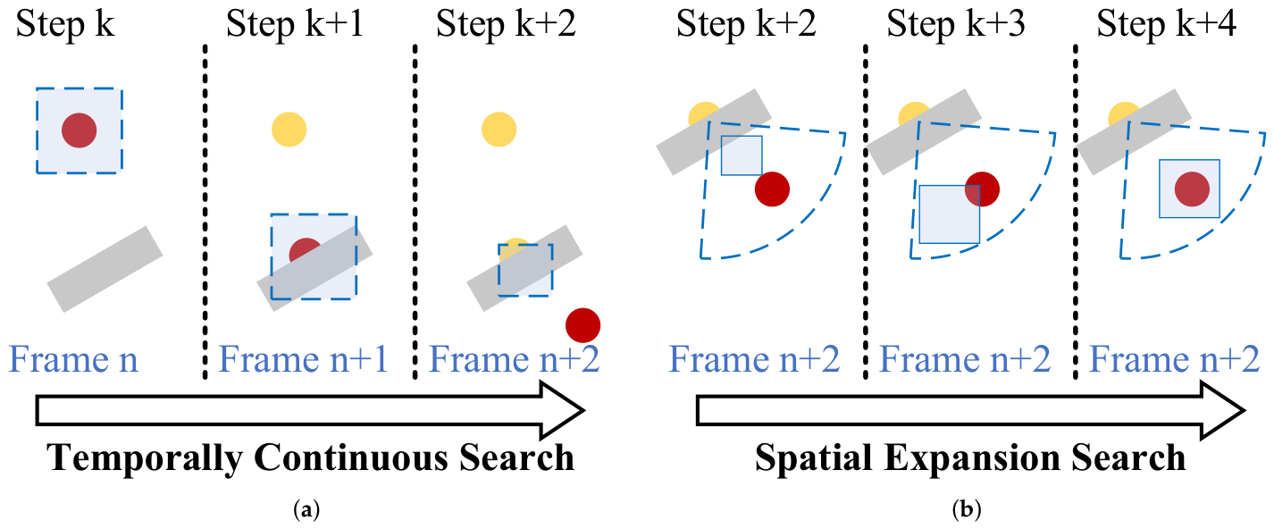
Figure 8.
Each step of temporally continuous search crops the search region on a new frame, while spatial expansion search crops the search region at different positions within the same frame, thereby reducing the computational burden associated with extensive searches required for tracking recovery. Arrows indicate temporal changes, yellow dots denote historical target positions, red dots denote the true target positions, blue dashed boxes indicate search ranges, and shaded boxes indicate the actual search regions. (a) Temporally continuous search. (b) Spatial expansion search.
Figure 8.
Each step of temporally continuous search crops the search region on a new frame, while spatial expansion search crops the search region at different positions within the same frame, thereby reducing the computational burden associated with extensive searches required for tracking recovery. Arrows indicate temporal changes, yellow dots denote historical target positions, red dots denote the true target positions, blue dashed boxes indicate search ranges, and shaded boxes indicate the actual search regions. (a) Temporally continuous search. (b) Spatial expansion search.
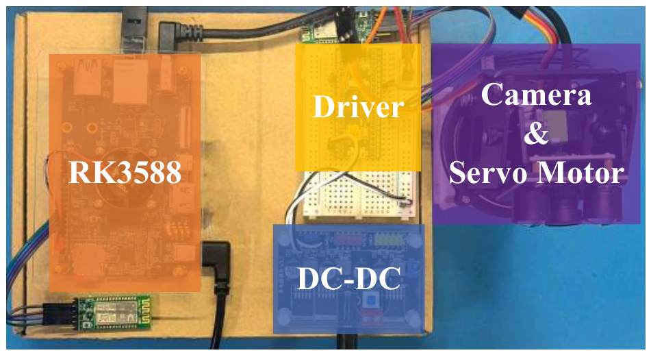
Figure 9.
Embedded hardware platform and several key components. The camera is equipped with steerable servos for object tracking or introducing motion disturbance.
Figure 9.
Embedded hardware platform and several key components. The camera is equipped with steerable servos for object tracking or introducing motion disturbance.
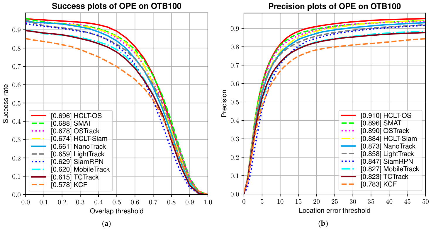
Figure 10.
Success plot and precision plot of OTB2015 with recently lightweight trackers. One-Pass Evaluation (OPE) refers to annotating targets only on the first frame. (a) Success plot. (b) Precision plot.
Figure 10.
Success plot and precision plot of OTB2015 with recently lightweight trackers. One-Pass Evaluation (OPE) refers to annotating targets only on the first frame. (a) Success plot. (b) Precision plot.
Figure 11.
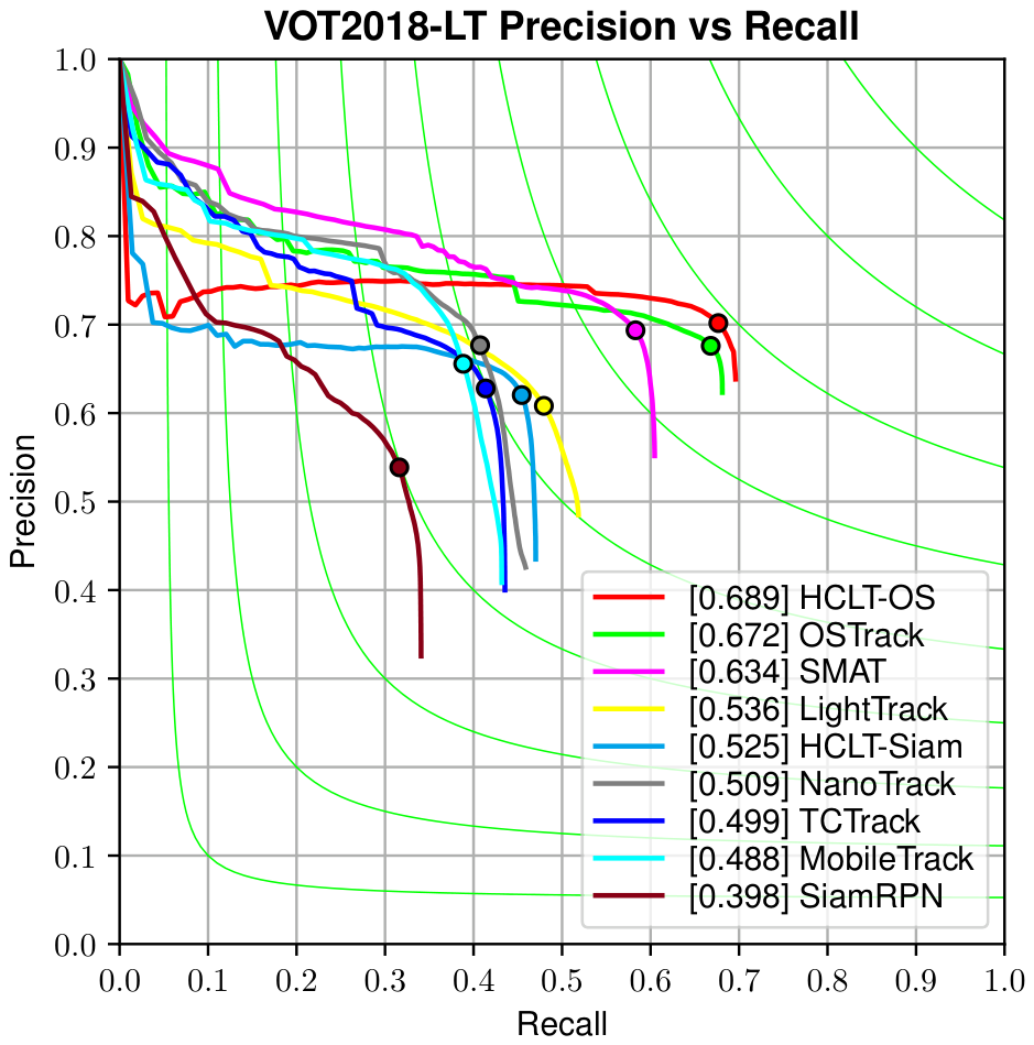
Precision–recall curve on VOT2018-LT dataset. Curves closer to the top-right corner indicate better long-term tracking performance. Dots on the curves denote the maximum F1-score points.
Figure 11.
Precision–recall curve on VOT2018-LT dataset. Curves closer to the top-right corner indicate better long-term tracking performance. Dots on the curves denote the maximum F1-score points.
Figure 12.
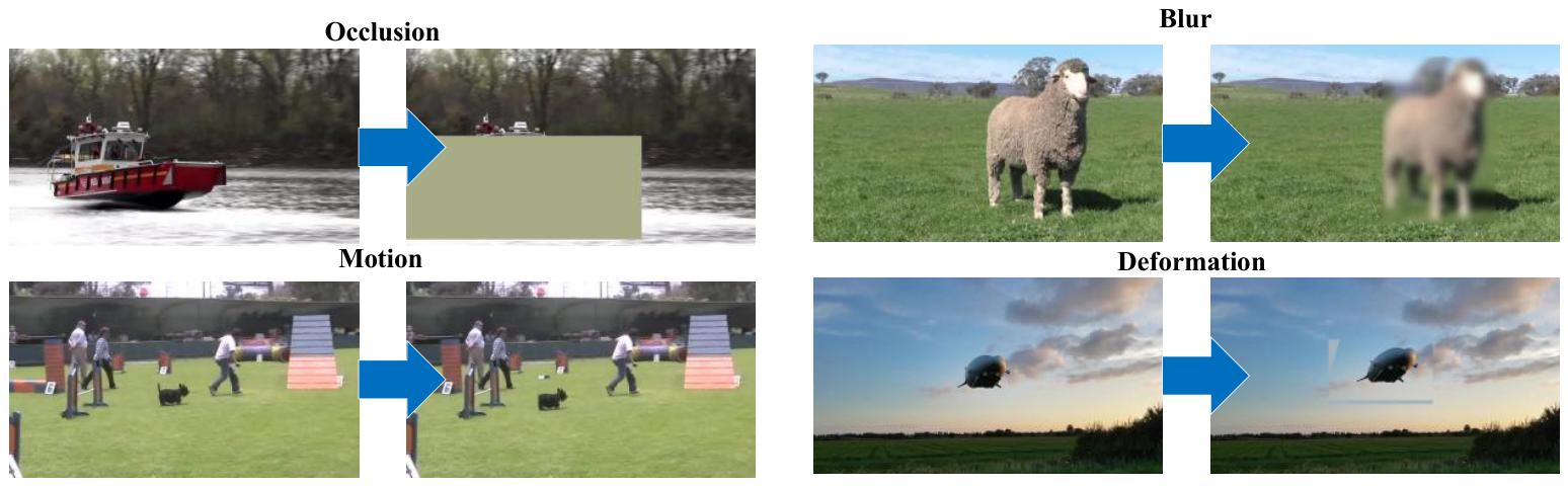
Visual effects of four representative disturbances.
Figure 12.
Visual effects of four representative disturbances.
Figure 13.
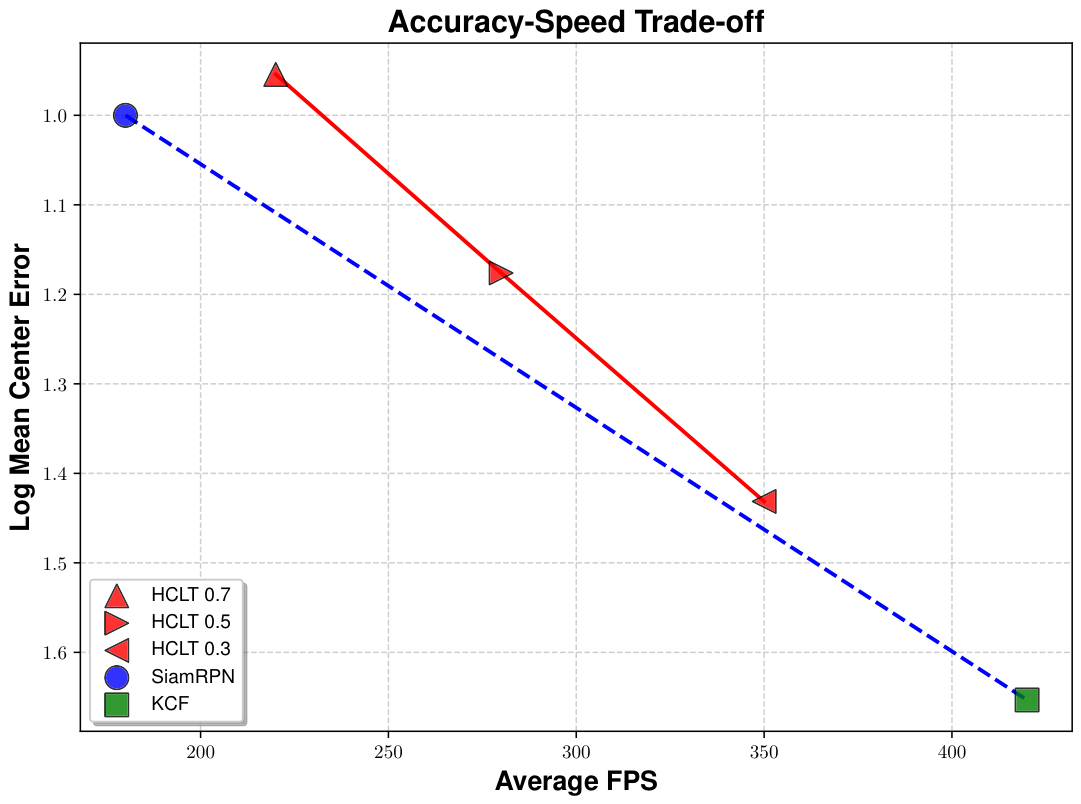
The accuracy of the tracker is evaluated using the logarithm of the mean center error, while its speed is assessed based on the average FPS. Trackers positioned closer to the top-right corner exhibit superior performance. The blue dashed line and red solid line are used only for a simple comparison of variation trends and have no actual meaning under the logarithmic coordinate.
Figure 13.
The accuracy of the tracker is evaluated using the logarithm of the mean center error, while its speed is assessed based on the average FPS. Trackers positioned closer to the top-right corner exhibit superior performance. The blue dashed line and red solid line are used only for a simple comparison of variation trends and have no actual meaning under the logarithmic coordinate.
Figure 14.
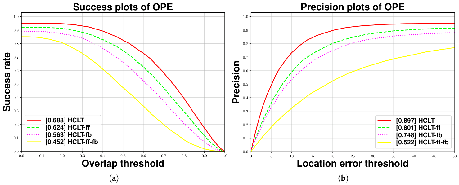
The performance was evaluated on the same video sequences, using the same success rate and precision metrics as defined in the OTB2015 benchmark. (a) Success plot. (b) Precision plot.
Figure 14.
The performance was evaluated on the same video sequences, using the same success rate and precision metrics as defined in the OTB2015 benchmark. (a) Success plot. (b) Precision plot.
Figure 15.
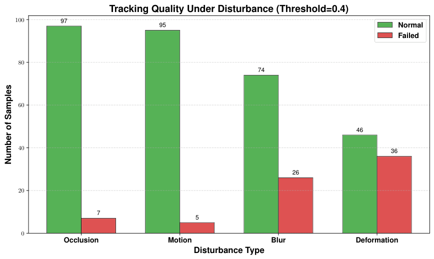
Judgment of tracking failure caused by different disturbances based on quality score.
Figure 15.
Judgment of tracking failure caused by different disturbances based on quality score.
Figure 16.
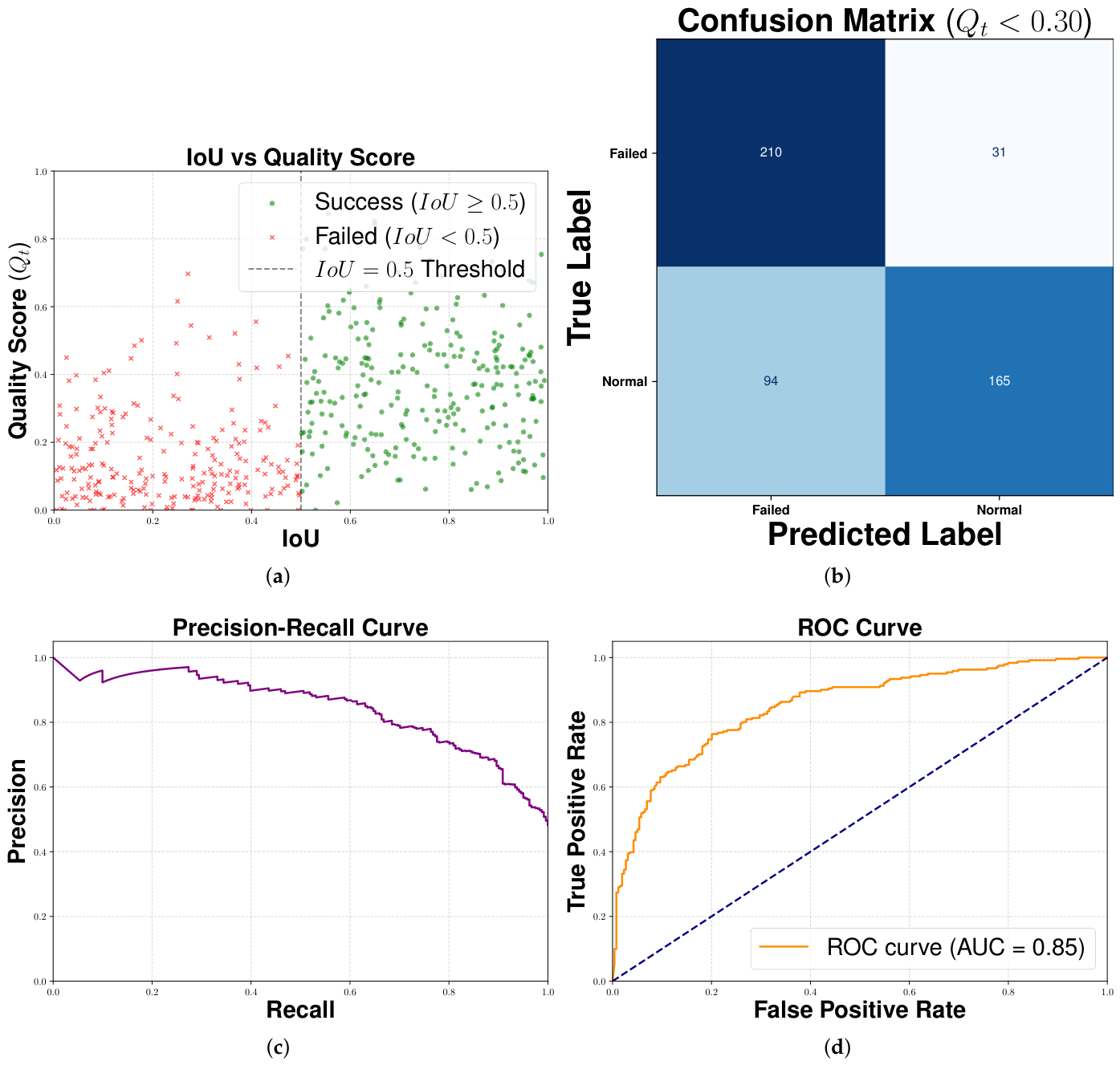
The evaluation metrics for some classifiers. (a) A scatter plot obtained from random sampling of video frames. Tracking is considered a failure when Intersection over Union (IoU) . (b) A confusion matrix of the true tracking state versus the predicted tracking state for randomly sampled instances, with tracking failure defined as the positive class. (c) A PR curve for quality estimation. (d) A ROC curve for quality estimation.
Figure 16.
The evaluation metrics for some classifiers. (a) A scatter plot obtained from random sampling of video frames. Tracking is considered a failure when Intersection over Union (IoU) . (b) A confusion matrix of the true tracking state versus the predicted tracking state for randomly sampled instances, with tracking failure defined as the positive class. (c) A PR curve for quality estimation. (d) A ROC curve for quality estimation.
Figure 17.
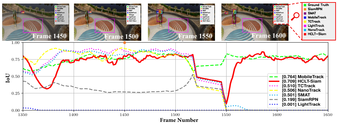
The tracker outputs bounding boxes along with the corresponding IoU curves for these frames. The curves have been smoothed.
Figure 17.
The tracker outputs bounding boxes along with the corresponding IoU curves for these frames. The curves have been smoothed.
Figure 18.
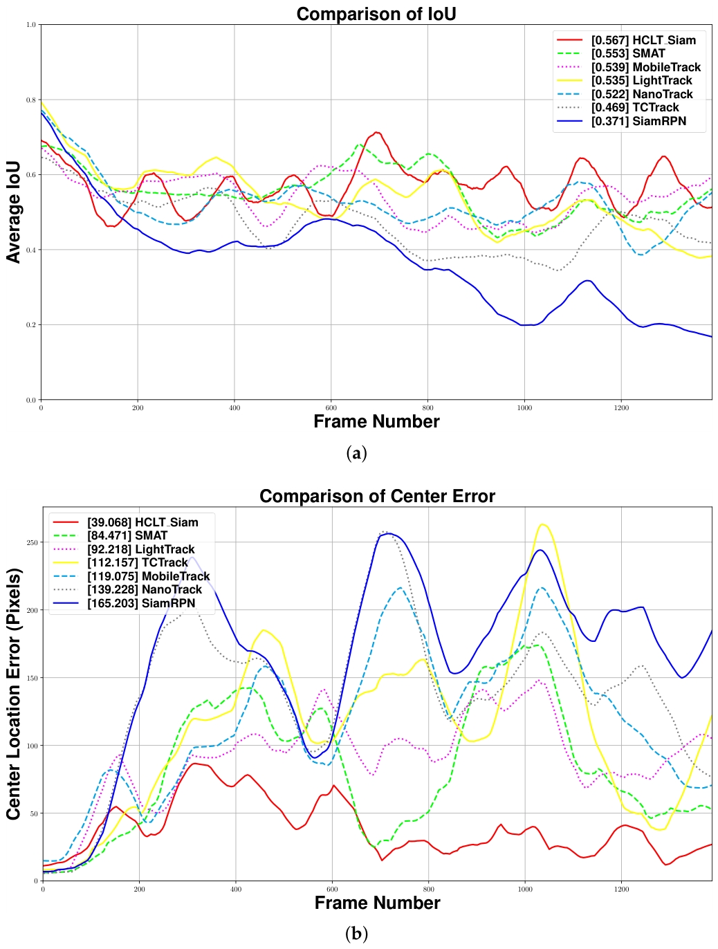
(a) Average IoU across multiple video sequences. (b) Average center error across multiple video sequences. The curves have been smoothed.
Figure 18.
(a) Average IoU across multiple video sequences. (b) Average center error across multiple video sequences. The curves have been smoothed.
Figure 19.
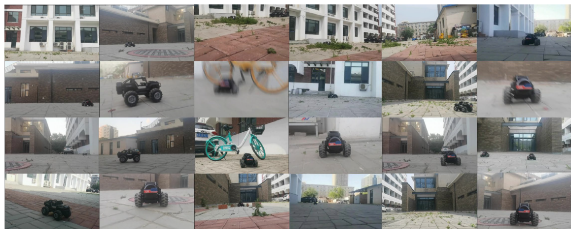
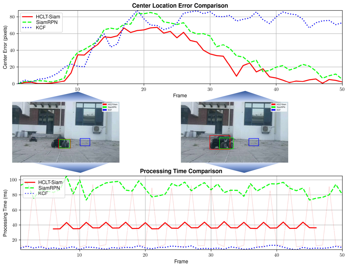
The video sequence obtained through real-time detection. The scene contains multiple types of disturbances.
Figure 19.
The video sequence obtained through real-time detection. The scene contains multiple types of disturbances.
Figure 20.
The center error and processing time for each frame in the video sequence. The red dashed line represents the actual processing time, while the red solid line denotes the smoothed average processing time.
Figure 20.
The center error and processing time for each frame in the video sequence. The red dashed line represents the actual processing time, while the red solid line denotes the smoothed average processing time.
Table 1.
Parameter initialization of the HCLT framework. Parameters are grouped by functional component.
Table 1.
Parameter initialization of the HCLT framework. Parameters are grouped by functional component.
| Parameter | Value | Description |
|---|
| Quality Estimation |
| | 0.80 | EMA smoothing coefficient |
| | 0.6 | Detector response normalization constant |
| | 0.5 | Feature retention penalty strength |
| K | 15 | Sliding window length for |
| | 10 | Look-back offset for feature retention change |
| Warmup frames | 20 | Frames before quality evaluation activates |
| Hysteresis State Machine |
| | 0.30 | Instantaneous quality threshold for “bad” frame |
| | 0.50 | Instantaneous quality threshold for “good” frame |
| | 8 | Consecutive bad frames to enter LOST |
| | 3 | Consecutive good frames to exit LOST |
| Quality-Gated Detector Switching |
| | 0.40 | Suppress FD when drops below |
| | 0.65 | Resume FD when recovers above |
| | 30–60 | Target frame rate (FPS) for speed-aware interleaving |
| Feature Tracker (Feedforward) |
| | 30 | Maximum feature points |
| | 5 | Minimum feature points for offset correction |
| | 15 × 15 | Lucas–Kanade window size |
| | 0.15 | Feedforward correction weight |
Table 3.
Precision, recall, and F1-score on VOT2018-LT. Trackers are ranked by F1-score in descending order.
Table 3.
Precision, recall, and F1-score on VOT2018-LT. Trackers are ranked by F1-score in descending order.
| Tracker | Precision | Recall | F1 |
|---|
| HCLT-OS | 0.702 | 0.677 | 0.689 |
| OSTrack | 0.676 | 0.668 | 0.672 |
| SMAT | 0.694 | 0.583 | 0.634 |
| LightTrack | 0.608 | 0.479 | 0.536 |
| HCLT-Siam | 0.620 | 0.454 | 0.525 |
| NanoTrack | 0.677 | 0.407 | 0.509 |
| TCTrack | 0.628 | 0.414 | 0.499 |
| MobileTrack | 0.656 | 0.388 | 0.488 |
| SiamRPN | 0.539 | 0.316 | 0.398 |
Table 4.
Performance comparison between baseline trackers and the proposed Hybrid framework. All tests are conducted on the CPU. The FD in all Hybrid Framework entries is KCF; therefore, the KCF row is marked with “—” because its hybrid result is already represented as the common FD.
Table 4.
Performance comparison between baseline trackers and the proposed Hybrid framework. All tests are conducted on the CPU. The FD in all Hybrid Framework entries is KCF; therefore, the KCF row is marked with “—” because its hybrid result is already represented as the common FD.
| Trackers | Base | Hybrid Framework |
|---|
| Succ | Prec | FPS | AUC | Pre | FPS |
|---|
| OSTrack | 0.678 | 0.890 | 7 | 0.672 | 0.885 | 32 |
| DaSiamRPN | 0.658 | 0.880 | 13 | 0.665 | 0.881 | 43 |
| SiamRPN | 0.629 | 0.847 | 11 | 0.642 | 0.861 | 41 |
| SiamFC | 0.586 | 0.772 | 28 | 0.601 | 0.812 | 63 |
| KCF | 0.578 | 0.783 | 407 | — | — | — |
Table 5.
FPS comparison between HCLT and other trackers. The video resolution is 720p.
Table 5.
FPS comparison between HCLT and other trackers. The video resolution is 720p.
| Tracker | FPS |
|---|
| HCLT | 39 |
| NanoTrack | >60 |
| LightTrack | 33 |
| TCTrack | 40 |
| SMAT | 45 |
| MobileTrack | 22 |
| SiamRPN | 9 |