Article

A Hybrid Closed-Loop Tracker Fusing a Kalman Filter State Observer for Fast and Robust Embedded Visual Tracking

1
School of Electrical and Information Engineering, Tianjin University, Tianjin 300072, China
2
School of Information Technology Engineering, Tianjin University of Technology and Education, Tianjin 300222, China
*
Author to whom correspondence should be addressed.
Electronics 2026, 15(11), 2276; https://doi.org/10.3390/electronics15112276
Submission received: 15 April 2026 / Revised: 12 May 2026 / Accepted: 19 May 2026 / Published: 25 May 2026
(This article belongs to the Special Issue Advances in Visual Tracking: Emerging Techniques and Applications)

Abstract

Visual object tracking finds extensive application in real-time video analysis on edge devices, yet faces dual challenges: decreased speed due to limited computational resources and weak anti-disturbance capability in complex scenarios. This paper proposes the Hybrid Closed-Loop Tracker (HCLT) to enhance both speed and robustness of embedded visual tracking. HCLT integrates high-precision and high-speed trackers to make real-time performance controllable, while a Kalman filter is employed for state observation and feedback. Within this closed-loop framework, we introduce motion and feature point information as supplementary states and further design mechanisms for adaptive search region adjustment and tracking recovery. Our methods effectively mitigate the impact of external disturbances. Experimental results demonstrate that HCLT further improves both speed and robustness on the basis of high-performance trackers, achieving high tracking accuracy across multiple public benchmark datasets. It demonstrates excellent anti-disturbance performance, particularly in challenging scenarios such as blur and occlusions, while maintaining frame rates exceeding 35 frames per second (FPS) at 720p resolution when deployed on an RK3588 embedded device, thus representing a significant improvement over deep neural network trackers.

1. Introduction

Visual Object Tracking (VOT) aims to continuously and accurately locate a pre-specified target within a video sequence and is generally referred to as Single Object Tracking (SOT). It is widely applied in video analysis for embedded scenarios, including pedestrian tracking [1,2], industrial robotics [3], and aerial drones [4,5,6]. However, VOT in embedded systems faces two major challenges: (1) limited computational capacity and resources struggle to support computationally intensive state-of-the-art (SOTA) tracking algorithms, making real-time tracking unattainable; (2) common disturbing factors in real-world tracking, such as motion blur, target deformation, and occlusion, often lead to degraded tracking performance or even failure. Therefore, trackers suitable for embedded devices must achieve an effective balance between speed and robustness to adapt to complex and dynamic real-world application scenarios under computational constraints.
Current mainstream trackers, predominantly based on the tracking-by-detection (TBD) paradigm, fall into two categories: Correlation Filter (CF) and Deep Learning (DL) methods [7,8]. CF methods leverage Fourier-domain operations for high speed but lack robustness against disturbances. In contrast, DL-based trackers (e.g., Siamese networks [9]) have become the standard for high precision but incur heavy computational costs. Despite efforts to compress the model, DL trackers often waste resources by recomputing deep features for every frame, regardless of tracking quality. We usually select models with lightweight convolutional neural networks as backbones as such solutions are more mature and can run stably on embedded devices.
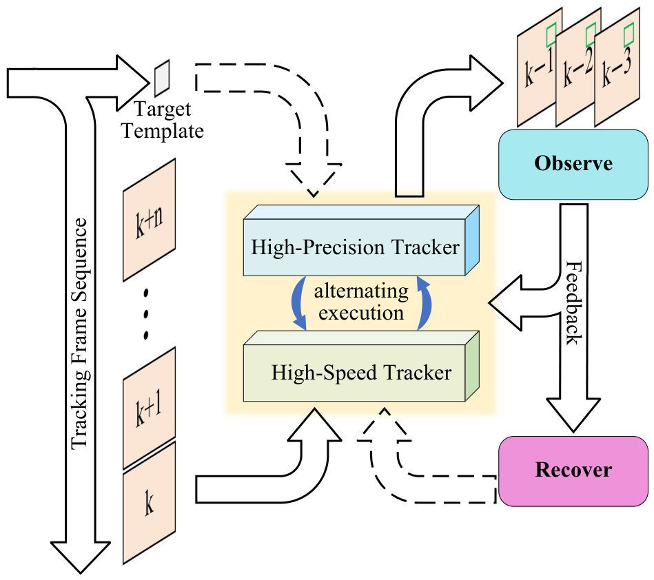
To bridge the gap between efficiency and robustness, we propose the Hybrid Closed-Loop Tracker (HCLT), as visualized by Figure 1. HCLT is a VOT general framework that overcomes the aforementioned shortcomings through three technical components: (1) a hybrid-tracker framework that integrates high-accuracy/low-speed and low-accuracy/high-speed trackers, allowing for dynamic computational load adjustment to satisfy real-time constraints; (2) a state observation-feedback mechanism that assesses tracking quality via motion prediction and feature point detection to optimize search strategies on the fly; (3) a recovery mechanism that triggers a resource-efficient distracted search strategy to recapture the target when the quality of tracking degrades. Furthermore, our ablation experiments demonstrate that the HCLT framework effectively enhances tracker performance, and extensive evaluations show that our approach outperforms several high-performance DL-based trackers in frame rate while maintaining competitive accuracy. Specifically, real-world testing on the RK3588 platform confirms robust performance at over 35 FPS.
The main contributions of this article are summarized as follows:
  • Hybrid Tracking Framework: A general framework that integrates high-accuracy and high-speed trackers is proposed, enabling dynamic computational load adjustment to satisfy real-time constraints on embedded devices. The framework transforms the tracking process into a controllable system where the detector switching, search region, and target scale are all regulated through explicit mechanisms.
  • Closed-Loop Observation–Feedback–Feedforward–Recovery Mechanism: Inspired by control system theory, we design a unified mechanism comprising: (a) a Kalman-filter-based state observer that propagates temporal motion information across frames via feedback; (b) a feedforward channel that exploits pixel-level spatial cues (feature point geometry) to correct the fast detector output in the current frame; (c) a quality-aware recovery strategy that triggers a distracted search to recapture the target when tracking quality degrades.
The remainder of this paper is organized as follows. Section 2 reviews related work on tracking-by-detection, evaluation and recovery mechanisms, and multi-tracker complementarity. Section 3 presents the proposed HCLT method in detail, including the hybrid framework, the tracking state observer, the feedforward–feedback search region control, and the distracted search recovery mechanism. Section 4 reports experimental results on benchmark datasets, ablation studies, long-term tracking, and real-time embedded testing. Section 5 provides a discussion of the results and limitations. Section 6 concludes the paper.

2. Related Works

2.1. Tracking by Detection

Converting a tracking task to a single-frame object detection task is a common design approach for tracking. In SOT, detection is typically performed only around the target, i.e., within the search region [7]. Correlation filters represent one of the most classic categories of such trackers. Since D.S. Bolme et al. [10] first proposed the MOSSE filter, numerous researchers have conducted extensive studies to enhance the performance of such trackers [5,11,12]. However, their limited feature representation capability often leads to poor robustness under complex conditions.
Siamese-based trackers use deep learning to extract high-level features, resulting in significantly improved accuracy and robustness, and have repeatedly achieved SOTA performance [9]. For example, Li et al. [13] proposed the SiamRPN, which integrates a weight-sharing feature extraction network with a region proposal network, thus achieving notable advantages in both accuracy and efficiency. Subsequent trackers have further refined the Siamese network architecture through various improvements, enhancing the feature representation of network [14,15,16,17] or using lightweight components [18,19].
Despite these advances, most existing trackers maintain a single-structure design, making it challenging to balance accuracy and efficiency in practical tracking scenarios, thus lacking flexibility. In contrast, our proposed tracker framework implements a hybrid-tracker design, allowing adaptive adjustment based on computational resources, task requirements, and tracking quality. This general-purpose tracker architecture is specifically tailored to meet the demands of real-time tracking on embedded devices.

2.2. Evaluation and Recovery Mechanisms in Tracking

Trackers designed under the TBD paradigm essentially perform target detection within a search region. However, the updating of the search region and the regularization of target position and size are typically pre-designed, thus lacking an effective evaluation mechanism and a reliable recovery method after tracking failure.
Regarding the evaluation mechanisms, Xu et al. [20] pointed out that anchor-based similarity scoring in region proposal networks suffers from prior bias and inaccuracies. They improved the fully convolutional network and introduced a separate quality assessment branch. Choi et al. [21] introduced perturbations by randomly erasing multiple regions in the image to obtain a more accurate model confidence state.
For recovery after tracking failure, Ma et al. [22] proposed decomposing long-term tracking into translation and scale estimation, incorporating temporal context modeling based on correlation filters and a random fern-based re-detection mechanism. This provided a classical framework for handling target disappearance and reappearance. Huang et al. [23] used a simple yet effective global search method, ensuring that frames where tracking fails do not affect subsequent search regions or tracking results. Choi et al. [21] abandoned computationally expensive global sliding windows in favor of randomly sampling multiple regions in the image for detection, applying spatiotemporal constraint penalties to potential targets.
Although these evaluation and recovery strategies are effective, they are implemented internally within a specific tracker, lack universality, and often introduce additional computational overhead. In contrast, our framework mimics the principles of a feedback control system by implementing evaluation and recovery mechanisms through a separate observation-feedback-recovery channel. This approach improves tracking stability while maintaining high computational efficiency.

2.3. Multi-Tracker Complementarity

Multi-tracker complementarity is a widely adopted optimization strategy capable of further enhancing tracking performance, potentially even surpassing single SOTA trackers [24]. Bailer et al. [25] introduced a Passive Fusion approach that operates without altering internal tracker states. This seminal work demonstrated that fusing multiple trackers consistently outperforms individual ones, establishing a lasting impact on the field. Similarly, Fan et al. [26] proposed the pioneering Parallel Tracking and Verifying (PTAV) framework. By decoupling and delegating tasks to a high-precision tracker and a high-speed tracker, respectively, PTAV achieves remarkable performance in real-time tracking. More recently, Dunnhofer et al. [27] designed CoCoLoT, a framework that combines the characteristics of complementary visual trackers, achieves enhanced long-term tracking performance by online selection of the best-performing tracker, and corrects the performance of failed trackers.
However, these existing multi-tracker methods typically increase computational overhead and are primarily evaluated offline using datasets. Consequently, there is no reliable hybrid tracking solution for embedded systems. To bridge this gap, we propose a hybrid tracker designed to reduce computational load, with its performance validated through online testing on embedded hardware.

3. Method

3.1. Framework for Hybrid Tracking

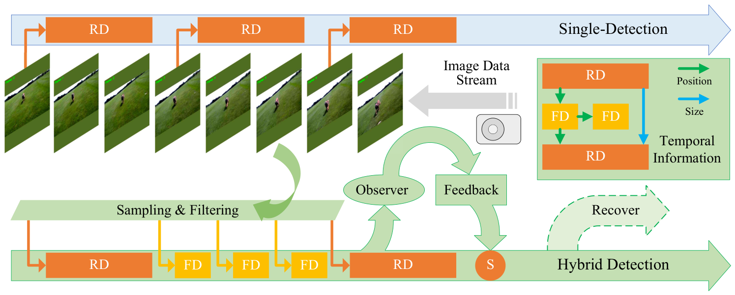
The hybrid tracking framework makes computational load controllable, which is also key to speed improvement. As shown in Figure 2, we employed two types of detectors, a reliable detector (RD) and a fast detector (FD), both of which are extracted from the TBD tracker. Specifically:
  • RD is typically extracted from deep neural network trackers, demonstrating high accuracy and stability during tracking, but its high computational complexity makes it difficult to achieve real-time performance on resource-constrained platforms.
  • FD is based on faster tracking methods, such as the correlation filter. Compared to RD, it incurs very low computational costs and meets real-time requirements in embedded computing, but its tracking performance declines significantly when faced with severe disturbance.
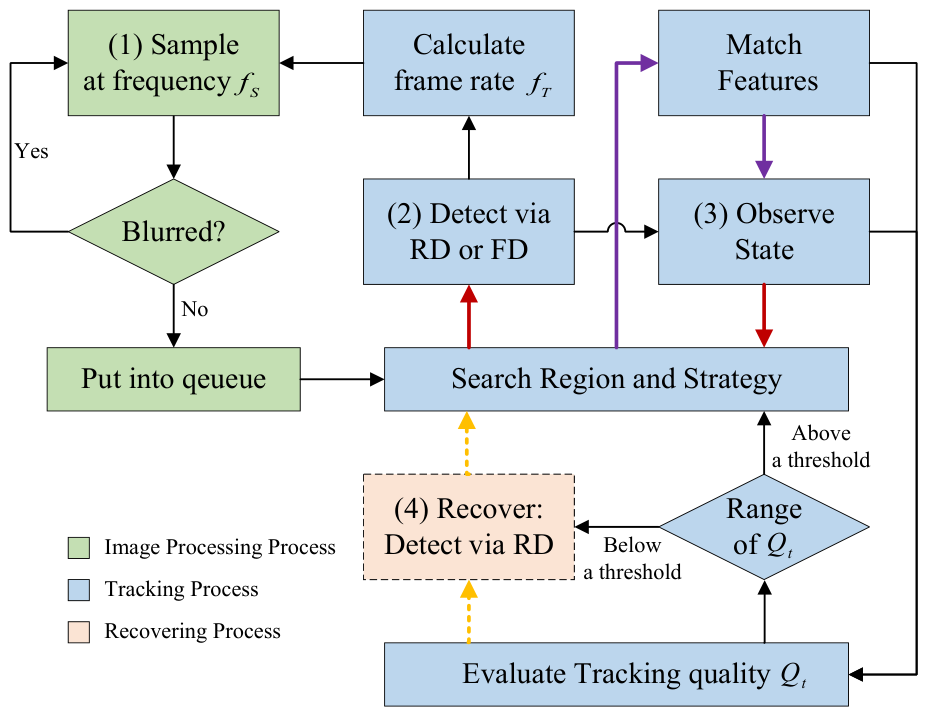
Our framework is similar to [26], but RD and FD alternate execution in different time slices within the same process, resulting in lower and controllable computational overhead. When tracking is stable, the frequency of FD usage increases. Figure 3 illustrates the overall workflow of HCLT, which can be divided into the following four main components:
  • Sampling and Preprocessing: An asynchronous process buffers the incoming image stream and estimates the camera frame rate f C = 1 / Δ t ¯ C , where Δ t ¯ C is the moving average of inter-frame intervals. Images are sampled at an adjustable frequency f S = min ( f C , f T + Δ f ) , where f T is the tracking frame rate fed back from the main process and Δ f is a small margin to prevent queue overflow. Each sampled frame undergoes a Fast Fourier Transform (FFT) to compute a blur metric B f f t ; frames with B f f t exceeding a preset threshold are discarded, while valid frames are enqueued for the main tracking process.
  • Target Detection and Tracking Execution: The main process retrieves valid frames from the queue and invokes a switching module S to select either RD or FD for the current frame. The switching decision is governed by two factors:
    • Speed-aware interleaving: Let t ¯ R D and t ¯ F D denote the exponentially smoothed processing times of RD and FD, respectively. When RD alone cannot meet the target frame interval τ t a r g e t = 1 / f t a r g e t , FD is interleaved every N frames, where N = ( t ¯ R D t ¯ F D ) / ( τ t a r g e t t ¯ F D ) .
    • Quality gate: When the tracking quality Q t drops below a suppression threshold τ l o w , FD usage is suppressed to prevent error propagation through FD’s RD-dependent template update. Normal interleaving resumes only when Q t recovers above a higher threshold τ h i g h , forming a hysteresis that prevents oscillation.
    Additionally, FD detections are protected by a drift guard: if the detection center deviates from the TSO-predicted position by more than γ times the target diagonal ( γ = 3.0 ), the output is anchored back to the predicted position with c d e t overridden to 0.3 . This prevents large excursions of the correlation filter during partial occlusion or rapid appearance changes. After detection, the tracking frame rate f T = 1 / t ¯ t r a c k is computed, where t ¯ t r a c k is the exponentially smoothed per-frame processing time, and is fed back to adjust f S in Stage 1.
    The complete detector switching policy is formally defined as a rule-based system combining the above two factors. At each frame, the switching module S operates as follows. First, a speed-driven baseline determines the nominal FD interleaving interval N via N = ( t ¯ R D t ¯ F D ) / ( τ t a r g e t t ¯ F D ) , where the smoothed per-detector processing times t ¯ R D and t ¯ F D are updated online. Second, a quality-driven gate overrides this schedule: when Q t < τ l o w , FD usage is suppressed regardless of the nominal schedule, forcing RD-only operation to prevent error propagation; the scheduled interleaving resumes only after Q t recovers above τ h i g h . The asymmetric hysteresis ( τ h i g h τ l o w = 0.25 ) ensures stable switching without oscillation. All thresholds are fixed values determined through grid search and listed in Table 1.
  • State Observation and Feedback Regulation: This stage constitutes the core of the closed-loop design and operates through two parallel channels (detailed in Section 3.2 and Section 3.3):
    • Feedback channel: A 6-state Kalman filter propagates the target’s motion state x k = [ c x , c y , d , v c x , v c y , v d ] T across frames. The predicted center defines the search region for the next frame, incorporating camera motion compensation via the control input u k .
    • Feedforward channel: Feature points (FAST [28] corners) are detected within the search region and tracked across frames via Lucas–Kanade [29] optical flow. The mean displacement between the point cloud center and the detector output provides a spatial correction offset applied to FD detections. The normalized point count r f = M / M a v g (relative to a short window of prior frames) serves as an indicator of feature point retention.
    Together, the feedback channel provides temporal continuity while the feedforward channel injects spatial information from the current frame, jointly refining the search region for the next detection cycle.
  • Quality Evaluation and Tracking Recovery: A continuous tracking quality score Q t [ 0 , 1 ] is computed at each frame. The instantaneous quality is defined by a three-factor multiplicative structure:
    Q i n s t = clip c d e t θ p , 0 , 1 · 1 + H k 2 · exp λ · min ( Δ r f , 0 )
    where c d e t is the detector response peak, θ p is a normalization constant, H k [ 0 , 1 ] is the Bhattacharyya-based histogram similarity between the current detection and the initial template, Δ r f = r f ( k ) r f ( k τ ) is the change in feature point retention ratio (negative values indicate point loss), and λ controls the penalty strength. The final quality is obtained via Exponential Moving Average (EMA) smoothing with coefficient β : Q t = β Q t 1 + ( 1 β ) Q i n s t . A hysteresis state machine determines the tracking status: the state transitions to LOST after N b a d consecutive frames with Q i n s t < θ b a d , and recovers to NORMAL after M g o o d consecutive frames with Q i n s t θ g o o d . When LOST is declared, an isolated recovery process (Section 3.4.2) is triggered to re-detect the target via a velocity-guided fan-shaped search, without interrupting the main tracking loop.

3.2. Tracking State Observer

The TBD tracker converts tracking into single-frame detection, disregarding the continuity of motion. Drawing inspiration from modern control systems, we have designed a Tracking State Observer (TSO) to predict the target’s state and pass it to the next frame, serving as the feedback channel for the hybrid tracking framework. We use the Kalman Filter [30] to estimate target states in TSO, and its effectiveness in VOT has been empirically validated [31,32].
To simplify the computation, the target is assumed to maintain a constant velocity over short periods. The TSO recursively estimates the current velocity by the previous frame’s velocity and the current camera motion state. The bounding box is [ c x , c y , w , h ] , where c x and c y represent the center coordinates, and w and h denote the width and height of the bounding box. The target state in the frame k is defined by a 6-dimensional vector x k :
x k = c x c y d v c x v c y v d T
where d is the diagonal length ( d = w 2 + h 2 ), and v c x , v c y , v d are their respective velocities. Assuming a discrete time step Δ t , the filtering process follows a standard Prediction-Update cycle.

3.2.1. Prediction Step

The a prior state estimate x ^ k for frame k is calculated using the state transition matrix F and the posterior state estimate x ^ k 1 from frame k 1 , and compensated by the control input u k via the control matrix B :
x ^ k = F x ^ k 1 + B u k
with
F = 1 0 0 Δ t 0 0 0 1 0 0 Δ t 0 0 0 1 0 0 Δ t 0 0 0 1 0 0 0 0 0 0 1 0 0 0 0 0 0 1 , B = Δ t 0 0 0 Δ t 0 0 0 Δ t 1 0 0 0 1 0 0 0 1
u k = v c a m , x v c a m , y v c a m , s T
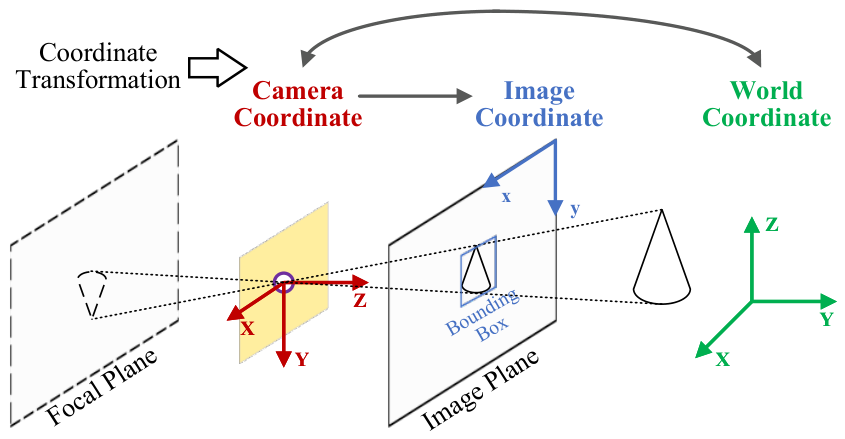
v c a m , x , v c a m , y , and v c a m , s respectively represent the x-axis velocity, the y-axis velocity, and the scaling velocity in the image coordinate system after transformation from camera motion, as illustrated in Figure 4. The transformation from physical camera motion to image-plane velocities is accomplished via the pinhole camera model.
(a) Camera Imaging Model. We adopt the standard pinhole camera model. For a 3D world point ( X , Y , Z ) T , its projection onto the image plane ( x , y ) T is given by:
x = f x X Z + c x 0 , y = f y Y Z + c y 0
(b) Intrinsic Matrix and Calibration. The intrinsic matrix K is:
K = f x 0 c x 0 0 f y c y 0 0 0 1
where f x , f y denote the focal lengths in pixels along the x and y axes, and ( c x 0 , c y 0 ) is the principal point. These parameters are obtained via standard checkerboard calibration [33].
(c) Conversion from Physical Velocity to Image Velocity. Consider a camera undergoing translational motion with instantaneous velocity V c a m = [ V X , V Y , V Z ] T in the world frame (where V Z > 0 corresponds to moving toward the scene). Taking the time derivative of the projection equations and assuming the tracked target lies near the optical axis ( X 0 , Y 0 ), the induced image-plane velocities are:
v c a m , x f x Z · V X , v c a m , y f y Z · V Y
For scale change, the apparent size (diagonal length d) of an object at depth Z is inversely proportional to Z. The time derivative yields:
v c a m , s = d Z · V Z
Thus, forward camera motion ( V Z > 0 ) reduces v c a m , s (negative contribution), which, combined with the negative entries in B , increases the predicted diagonal d, correctly reflecting the growth of the target’s apparent size.
In practice, for monocular 2D tracking where the absolute depth Z is unknown, the global inter-frame camera displacement is estimated directly from background optical flow: sparse feature points are detected in the background region (outside the target bounding box), tracked via Lucas–Kanade optical flow between consecutive frames, and the median displacement is used as a robust estimate of the image-plane velocity components v c a m , x and v c a m , y . For v c a m , s , it is estimated from the scale change of the background feature point constellation. For dataset evaluation where no physical camera motion exists, u k = 0 and the filter reduces to the standard constant-velocity model.
Let Q represent the process noise covariance. Then, the prior estimated covariance P k can be derived from the posterior covariance P k 1 of the previous frame as:
P k = F P k 1 F T + Q

3.2.2. Update Step

The measurement vector z k is obtained from the bounding box:
z k = c x , m c y , m d m T
The most critical step is to compute the Kalman gain K k , which determines the extent to which the new measurement should be trusted:
K k = P k H T ( H P k H T + R ) 1
where R is the measurement noise covariance matrix, and H is the observation matrix that maps the state space to the measurement space. Since velocity cannot be directly measured,
H = 1 0 0 0 0 0 0 1 0 0 0 0 0 0 1 0 0 0
The final posterior state estimate x ^ k and its error covariance P k are updated as
x ^ k = x ^ k + K k ( z k H x ^ k )
P k = ( I K k H ) P k

3.3. Control Effect on Search Region

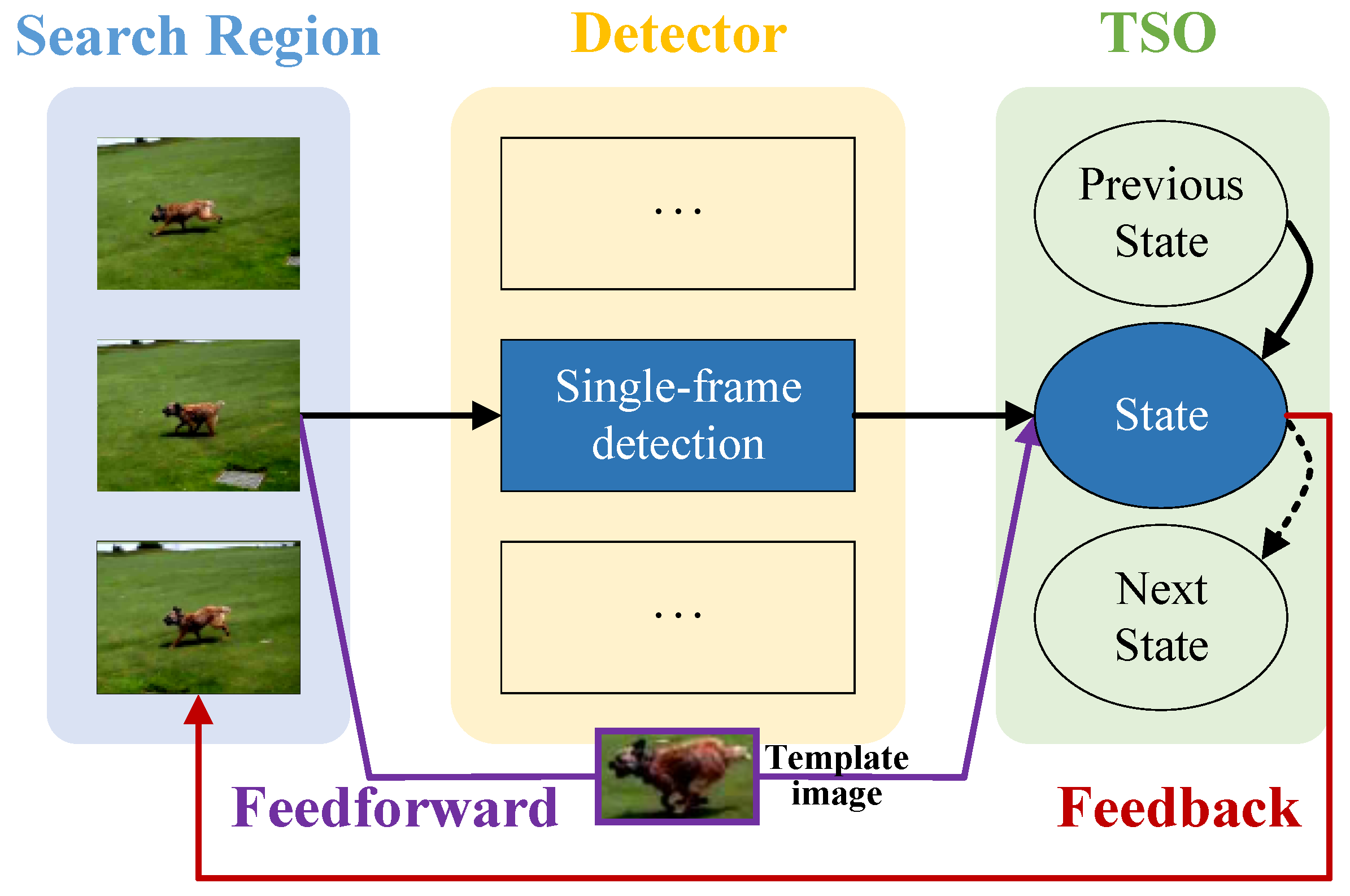
The TBD tracker focuses on a search region, which is updated using the target position from the previous frame and carries strong prior information [20]. Therefore, the update strategy is crucial to achieve stable tracking. We designed a search region adjustment method based on the HCLT framework, which is implemented through two channels, as illustrated in Figure 5. Our method employs raw spatial information—feature point detection and optical flow—as a lightweight target consistency check: the feedforward channel constrains excessive deformation and drift of the bounding box by anchoring the target center, while the feedback channel smooths the target motion trajectory and reduces jitter.
  • Feedforward: HCLT detects feature points (FAST corners) within the search region and tracks them via Lucas–Kanade sparse optical flow. The displacement between the feature point centroid and the detector output provides a spatial correction offset for the fast detector (FD). The number of surviving feature points also serves as a key signal for quality assessment.
  • Feedback: HCLT predicts the target’s center position in the next frame based on the motion state observed by the TSO, providing a more accurate search region for detection in the subsequent frame.
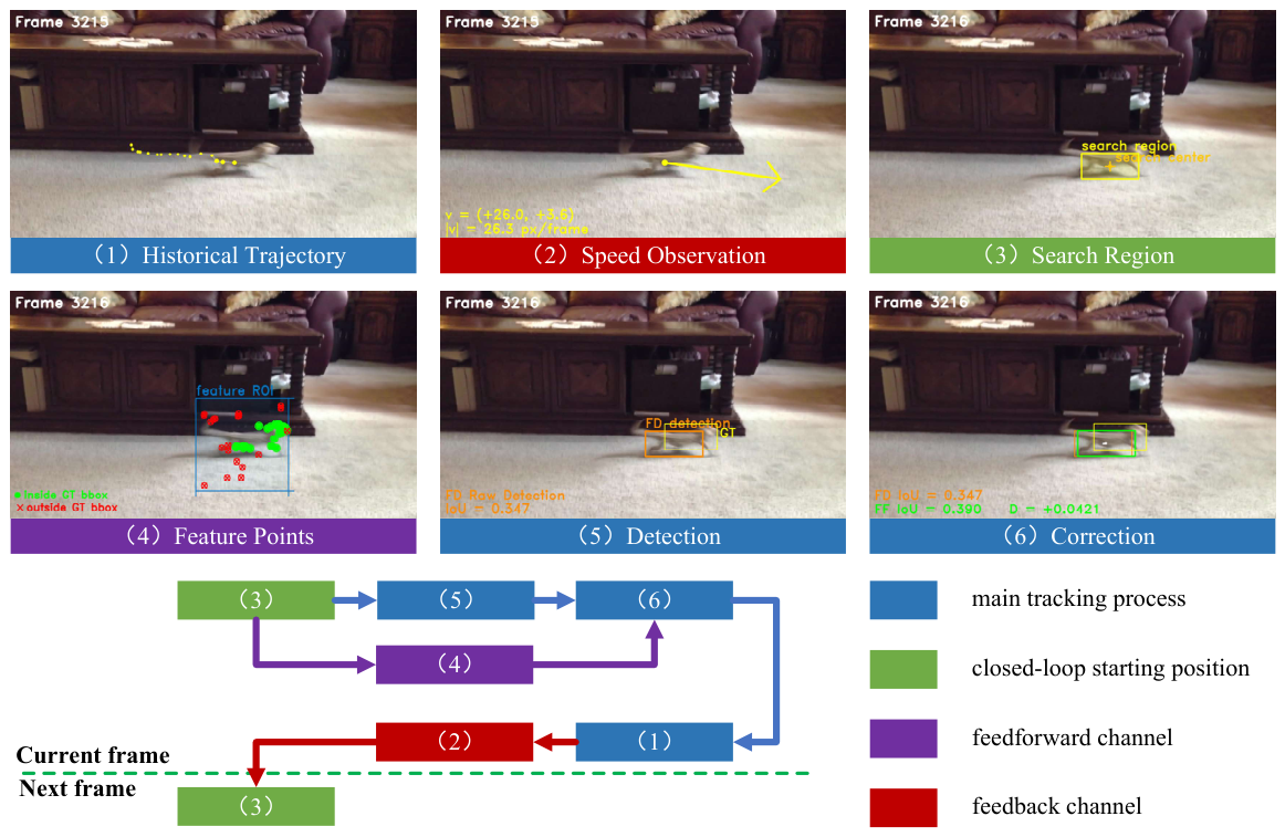
Algorithm 1 details the complete closed-loop per-frame tracking procedure, integrating detector switching, confidence extraction, feedforward correction, quality evaluation, and hysteresis-based recovery. Figure 6 displays a visual representation of this feedforward-feedback process. This search strategy operates as an independent external module of the detector. On the one hand, it enhances the stability of the tracking system by emulating the principles of a control system. On the other hand, it enables a general-purpose evaluation of tracking quality, which will be further discussed in Section 3.4.2.
Algorithm 1: HCLT Per-Frame Closed-Loop Tracking
Electronics 15 02276 i001

3.4. Distracted Search for Recovery

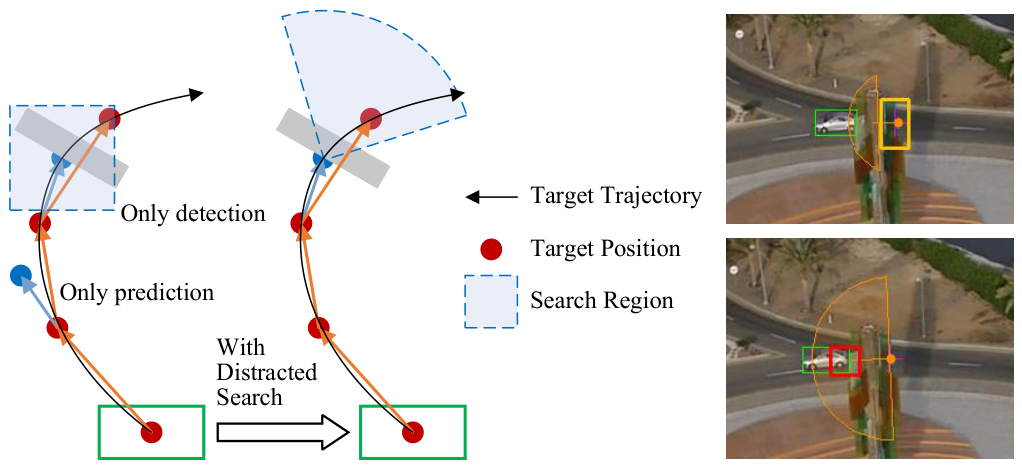
We designed a distracted search mechanism that initiates one or more sub-processes (distracted processes) to recover the target and does not interfere with the main tracking process. Distracted processes are typically activated when the tracking quality Q t falls below a predefined threshold. If Q t of the sub-process exceeds that of the main process, tracking is recovered from the sub-process. Otherwise, the sub-process will be released after a certain period. The mechanism relies on two key components: tracking quality Q t and the distracted search region.

3.4.1. Tracking Quality

The feature point retention ratio serves as the primary indicator of tracking continuity. Let M denote the number ( M k for frame k) of valid feature points tracked on the target at frame k. A reference baseline M a v g is maintained as a sliding-window average over a sliding window of length K:
M a v g ( k ) = 1 K i = 0 K 1 M k i , K = 15
When the target is occluded or lost, M drops sharply relative to M a v g , providing a responsive degradation signal. The feature point retention ratio is r f = min ( 1.0 , M / M a v g ) .
The overall tracking quality Q t combines three complementary signals into a multiplicative structure, as introduced in Stage 4 of the workflow. The instantaneous quality is:
Q i n s t = clip c d e t θ p , 0 , 1 · 1 + H k 2 · exp λ · min ( Δ r f , 0 )
where c d e t is the detector response peak—extracted as the Siamese cross-correlation score for RD and the correlation filter response peak for FD— θ p = 0.6 is a fixed normalization constant, H k [ 0 , 1 ] is the Bhattacharyya-based histogram similarity between the current detection and the initial template, and Δ r f = r f ( k ) r f ( k τ ) captures the change in feature retention over the look-back window. The parameter λ = 0.5 controls the penalty strength for negative Δ r f .
The final quality is obtained via EMA smoothing:
Q t = β Q t 1 + ( 1 β ) Q i n s t
with initial value Q 0 = 1.0 and smoothing coefficient β = 0.80 , corresponding to an effective temporal window of approximately 5 frames. During the warmup period (first 20 frames), Q t is clamped to a minimum of 0.9 .
A hysteresis state machine then determines the tracking status based on Q i n s t : the state transitions to LOST after N b a d consecutive frames with Q i n s t < θ b a d , and recovers to NORMAL after M g o o d consecutive frames with Q i n s t θ g o o d . The asymmetric design ( N b a d = 8 > M g o o d = 3 ) prevents oscillation at the decision boundary. All quality-related parameters were determined through grid search on a validation subset of OTB2015; a complete parameter initialization table is provided in Section 4.

3.4.2. Distracted Search Region

The distracted search mechanism operates as follows. When the hysteresis state machine declares a LOST state (Section 3.4.1), a recovery sub-process is spawned alongside the main tracking loop. The recovery process executes the following steps at each subsequent frame:
  • Fan-shaped feature accumulation. A fan-shaped search region is constructed in the current frame, centered at the predicted target position p p r e d ( k ) = p l o s s + v l o s s · k , where p l o s s is the target position at the time of loss, v l o s s is the smoothed velocity vector at loss, and k is the number of frames since loss. The fan is oriented along the velocity direction, with its angular span and radial extent expanding over time to gradually cover a larger search area:
    α k = α 0 + r α · k , α 0 = π / 6 , r α = π / 30
    R k = d t a r g e t · ( ρ 0 + r ρ · k ) , ρ 0 = 2.0 , r ρ = 0.5
    where α k is the half-angle of the fan at frame k, R k is the search radius, and d t a r g e t = w l o s s 2 + h l o s s 2 is the target diagonal length at the time of loss. The fan is bounded by the two rays at angles θ v e l ± α k , where θ v e l = arctan 2 ( v y , v x ) is the velocity direction. When the target area exceeds 30% of the image area or α k π , the search region degenerates to the full image. Up to M r e c = 80 FAST feature points are detected within the fan-shaped mask and stored in a frame buffer of maximum length 30.
  • Lucas–Kanade chain construction. To enable spatial projection across non-adjacent frames, a chain of LK optical flow transitions is maintained between consecutive buffered frames. Each transition records the correspondence between feature points in frames i and i + 1 , allowing any position in a past frame to be projected forward to the current frame via chained displacement vectors.
  • Feature clustering and candidate selection. Once at least M m i n a c c = 5 frames have been accumulated, the oldest buffered frame is selected for evaluation. Feature points in this frame are clustered using a distance threshold ε = w l o s s · h l o s s (i.e., the square root of the target area). Each cluster centroid defines a candidate search location. Clusters are evaluated sequentially, one per frame, to amortize computational cost.
  • Candidate verification and projection. At each candidate center, the RD (Siamese tracker) performs a detection with the search region size set to the target size at loss. The detection confidence is evaluated as Q c a n d = clip ( c d e t R D / θ p , 0 , 1 ) . If Q c a n d exceeds the maximum quality recorded during the loss period, the candidate is accepted. The detected position is projected from the evaluation frame to the current frame via the LK chain, and tracking is restored with the recovered bounding box. If no candidate in the current frame passes verification, the evaluator advances to the next buffered frame. When all buffered frames are exhausted, the process resumes accumulating new frames.
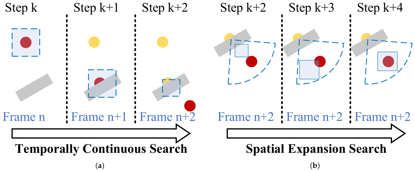
This design balances search thoroughness with computational efficiency: the expanding fan limits feature detection to a probabilistically motivated region, the frame-buffering and per-frame single-cluster evaluation amortize RD detection cost, and the LK chain enables correct spatial alignment of detections from past frames to the current time step. The expansion process of the fan-shaped search region is illustrated in Figure 7. Unlike temporally continuous recovery, HCLT does not perform frame-by-frame detection during recovery; instead, it searches multiple candidate regions within a single frame, as shown in Figure 8.

4. Experiment and Results

4.1. Implementation Details

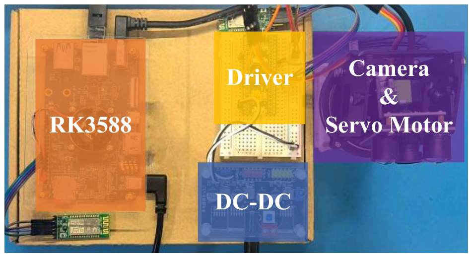
We conducted multiple experiments on HCLT to demonstrate the advantages of our framework. Depending on the hardware setup, the experiments in this section can be divided into simulation evaluation and embedded testing. Our simulation evaluation was performed on a PC equipped with an Intel Ultra 7 265K CPU, 16 GB RAM, and an NVIDIA RTX 5070 Ti GPU, CUDA 13.0. The embedded testing was carried out on an RK3588 platform with a built-in camera and 4 GB RAM, as illustrated in Figure 9.
In terms of algorithm selection, this paper adopts a variety of lightweight models designed for embedded visual tracking, together with several classical models for comparison. Two types of Hybrid Closed-Loop Trackers (HCLT) are adopted in the experiments. For HCLT-OS, OSTrack [34] is employed as the Reference Detector (RD); for HCLT-Siam, SiamRPN [13] with the AlexNet [35] backbone is used as the RD. All HCLT variants adopt the Kernelized Correlation Filter (KCF) [10] tracker with grayscale features as the Forward Detector (FD). All deep learning models are sourced from official releases and implemented based on PyTorch. Except for the SiamRPN model weights, which are obtained by training for 100 epochs on the GOT-10K [23] dataset, the weights of all other models adopt the officially released public weight files. All comparative results are tested under identical experimental environments.
The key parameters of the HCLT framework and their initialization values are summarized in Table 1. All parameters were determined through a grid search on a randomly selected 20-sequence validation subset of OTB2015, which optimizes for the area under the curve (AUC) metric under the one-pass evaluation protocol.
In our validation experiments, the framework showed moderate sensitivity to these default settings: small one-at-a-time perturbations around the calibrated values did not cause drastic performance drops, while noticeable degradation mainly appeared when multiple coupled thresholds were shifted away from their tuned ranges.
  • Simulation Evaluation: We evaluate the optimal performance as well as the performance improvement brought by the proposed HCLT method through HCLT-OS and HCLT-Siam.
    Section 4.2 evaluates the tracking framework on several benchmark datasets to assess its performance metrics.
    Section 4.3 presents ablation experiments aimed at demonstrating the impact of different modules and parameters of the tracking framework.
  • Embedded Testing: We test the robustness and real-time performance of the tracking framework on embedded devices via HCLT-Siam.
    Section 4.4 tests the long-term robustness and tracking recovery capability of the framework on a long-term tracking dataset.
    Section 4.5 demonstrates real-time tracking performance using a camera on the embedded platform.

4.2. Benchmark Results

4.2.1. OTB2015

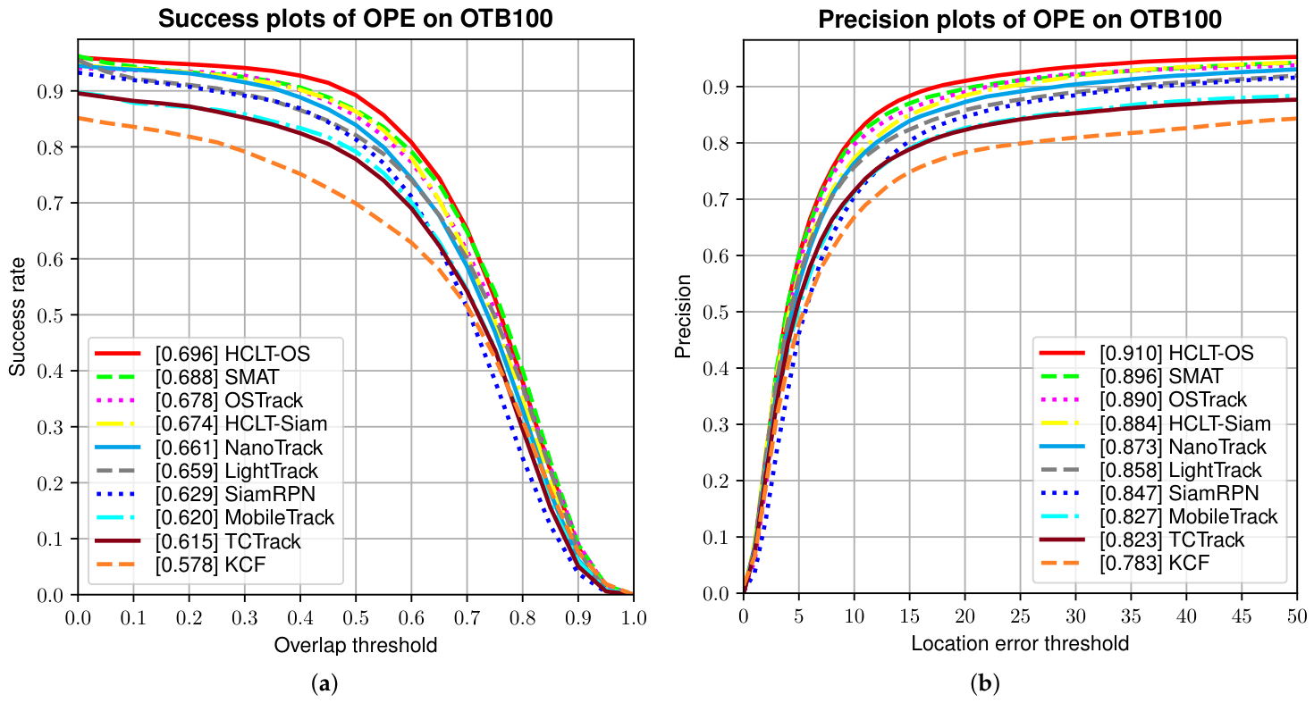
OTB2015 [36] contains 100 sequences that are collected from commonly used tracking sequences. The evaluation is based on two metrics: precision and success plot. The precision plot shows the percentage of frames where the tracking results are within 20 pixels of the target. The success plot shows the ratios of successful frames when the threshold varies from 0 to 1, where a successful frame means its overlap is larger than the given threshold. The area under the curve (AUC) of the success plot is used to rank the tracking algorithm.
In this experiment, our framework was compared with several representative trackers. As illustrated in Figure 10, HCLT-OS outperforms all the aforementioned comparison trackers and achieves further performance improvement on the basis of the original OSTrack. Meanwhile, HCLT-Siam also surpasses SiamRPN and KCF, which are adopted as its core components, thus demonstrating its capability to enhance tracker performance.

4.2.2. VOT2022

The VOT2022 [37] dataset consists of 128 videos. Performance is evaluated under the baseline protocol by Expected Average Overlap (EAO), Accuracy (A), and Robustness (R), which together measure the overall tracking capability. The test results on VOT2022 are shown in Table 2. HCLT-OS and HCLT-Siam achieve competitive performance against both classic and recently lightweight trackers, including OSTrack [34], SMAT [38], TCTrack [39], and MobileTrack [40].

4.2.3. VOT2018-LT

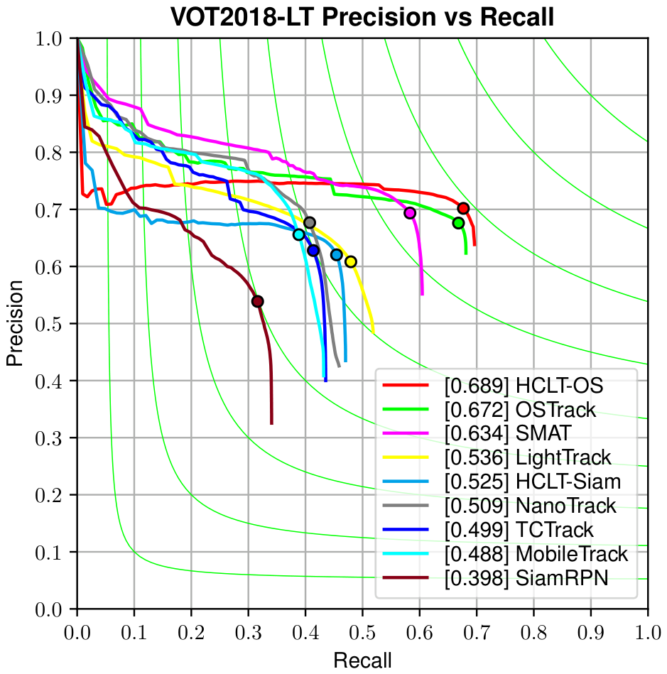
The VOT2018-LT dataset [41] extends the standard VOT evaluation to long-term sequences, where trackers must maintain target lock across hundreds of frames with full occlusions and target disappearance. A key metric in this benchmark is the precision–recall curve, which captures both the tracker’s detection accuracy and its re-detection capability after occlusion. The results on VOT2018-LT are presented in Figure 11 and Table 3.
Table 2. Results on VOT2022 baseline. Top-3 results of each dimension (column) are colored in red, green, and blue, respectively.
TrackersEAOAR
HCLT-OS0.5610.8060.850
HCLT-Siam0.4400.6940.772
OSTrack0.4950.7680.788
SMAT0.4780.7610.769
NanoTrack0.4110.6590.753
LightTrack0.3920.6820.703
TCTrack0.3400.6300.676
MobileTrack0.3350.6510.626
SiamRPN0.3130.5960.644
As shown in Figure 11, HCLT-OS achieves the best precision–recall trade-off, with its curve consistently positioned closer to the top-right corner compared to all other trackers. In terms of F1-score (Table 3), HCLT-OS ranks first (0.689), followed by OSTrack (0.672) and SMAT (0.634). The recall advantage is particularly noteworthy: HCLT-OS attains a recall of 0.677, substantially higher than SMAT (0.583). This demonstrates the effectiveness of HCLT’s distracted search recovery mechanism in re-detecting targets after long-term occlusions. HCLT-Siam, which shares the same SiamRPN detector, achieves an F1-score of 0.525—still outperforming SiamRPN (0.398) and remaining competitive with LightTrack (0.536). This confirms that the closed-loop framework provides consistent improvements over its underlying detector and enables flexible detector upgrading with measurable gains.

4.3. Ablation Study

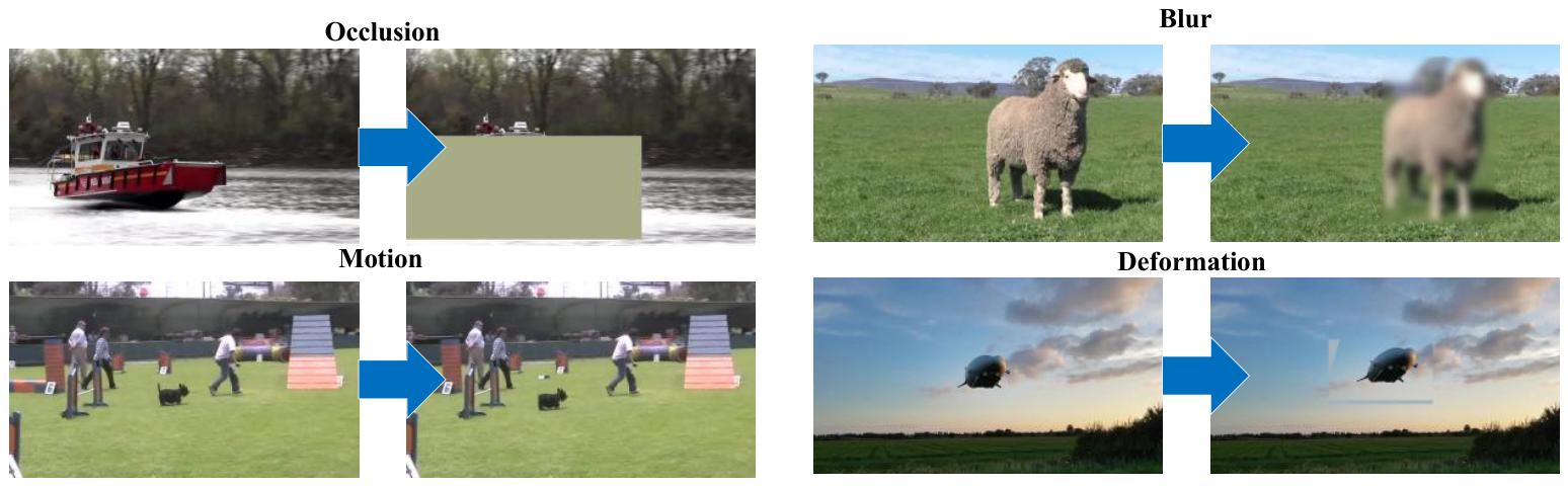
We selected 500 video sequences in which HCLT-Siam achieves stable tracking to test the functionality of each component of the tracking framework. During robustness testing, common real-world disturbance factors such as occlusion, motion, blur, and deformation were manually simulated, as shown in Figure 12. Unless otherwise specified, HCLT in this section refers to HCLT-Siam.

4.3.1. Hybrid Tracking Framework

We evaluate the performance gain of the proposed Hybrid tracking framework on multiple baseline trackers. Since these baseline trackers generally run at over 200 FPS on the GPU platform, it is difficult to trigger the automatic switching mechanism of the framework, making the FD barely functional. Therefore, all tests are conducted on the CPU.
The experimental results are listed in Table 4. The success rate (succ) and precision rate (prec) are evaluated on the OTB100 dataset, and KCF is adopted as the FD for all Hybrid tracking frameworks. The results demonstrate that the proposed Hybrid tracking framework can increase the frame rate by 2 to 3 times while maintaining or even slightly improving the tracking accuracy, achieving a remarkable acceleration effect.
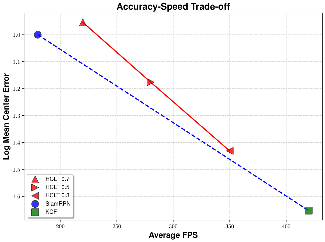
We further test the effect of manually controlling the usage frequency of FD on tracker precision. The results are shown in Figure 13, where HCLT 0.3 indicates that 30 percent of the frames in the entire tracking process used RD for detection; the same applies to the remaining terms. These results demonstrate that HCLT is faster than the original tracker SiamRPN and allows flexible performance adjustment. As the frequency of RD usage decreases, the accuracy of HCLT declines while the frame rate increases. It is noted that the absolute slope of the HCLT curve is greater than that of SiamRPN and KCF. This may be attributed to the fact that HCLT utilizes the more accurate RD for target scale updates, whereas FD detection does not perform scale updates during tracking.

4.3.2. Feedforward and Feedback

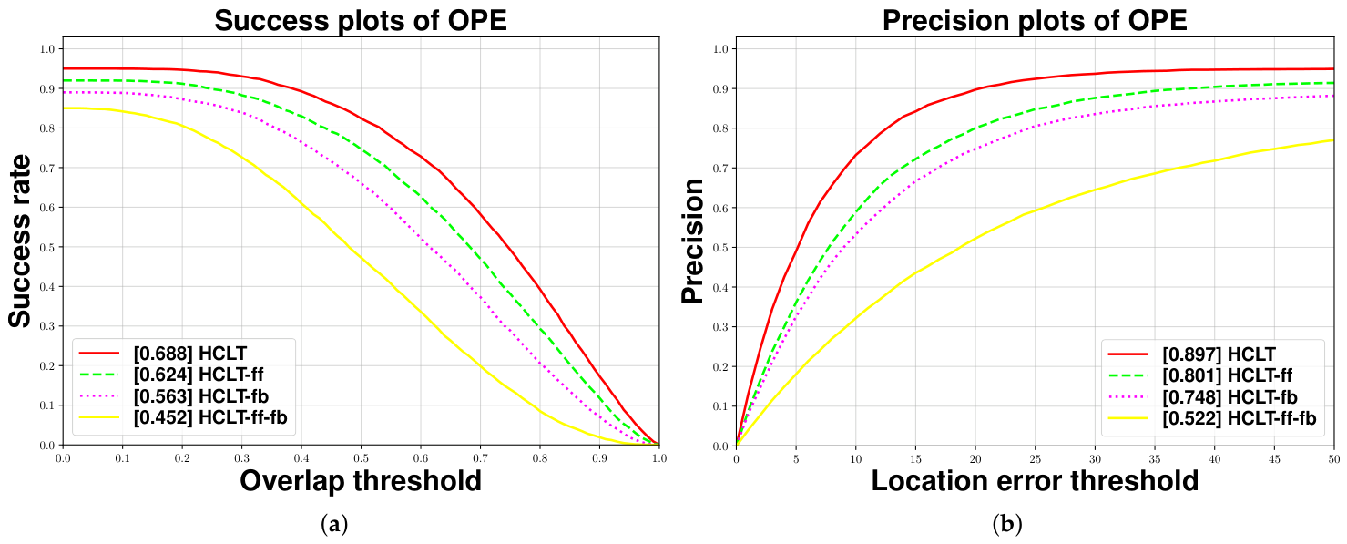
We evaluated the improvement of the feedforward-feedback regulation on tracking stability. We first conducted experiments using the complete HCLT framework and recorded the usage patterns of the two detectors. Keeping this pattern unchanged, we then removed either the feedforward or the feedback channel and repeated the experiments, selecting precision and success rate as evaluation metrics. The results are shown in Figure 14, where HCLT-ff denotes the HCLT framework without the feedforward mechanism; all other names follow the same convention. It can be observed that both feedforward and feedback contribute to enhancing the performance of HCLT. Additionally, we tested the operational speed under these four configurations. The experiments demonstrated that feedback has little impact on FPS, whereas the feedforward mechanism reduces FPS by approximately 15–20 frames. Specifically, the complete HCLT configuration achieves approximately 230 FPS on the simulation platform (GPU), and removing the feedforward channel increases this to approximately 250 FPS. The feedforward overhead is due to FAST feature detection and Lucas–Kanade optical flow computation. In practical applications, the feedforward regulation is typically applied every few frames.

4.3.3. Tracking Quality Estimation

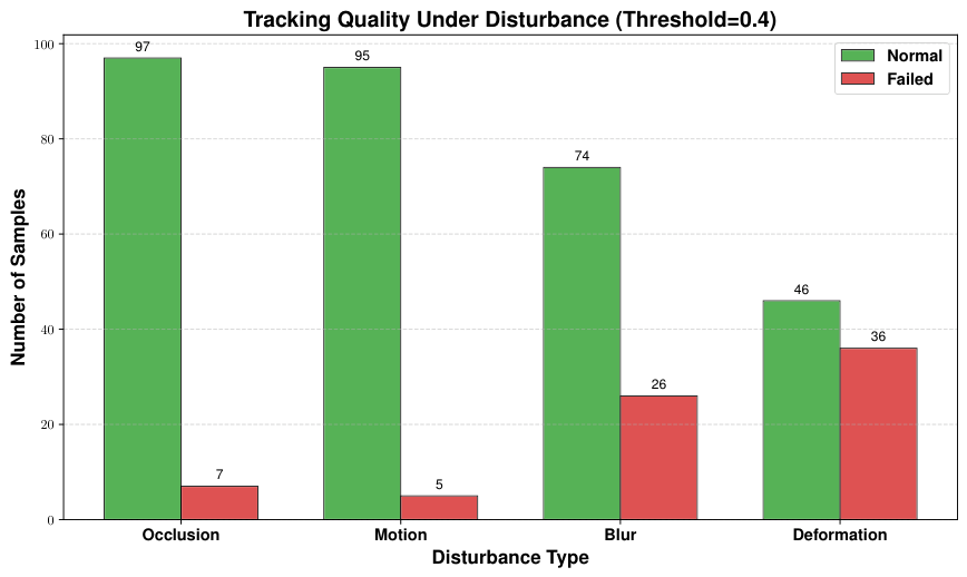
In HCLT, tracking quality Q t below a certain threshold is considered a tracking failure. We manually introduced four types of disturbances—occlusion, motion, blur, and deformation—into the selected video sequences. Using a threshold of 0.4, the resulting histogram (as shown in Figure 15) shows that disturbances causing target loss, such as occlusion and motion, are more likely to lead to a decline in Q t than disturbances such as blur or deformation, where the target remains within the search area.
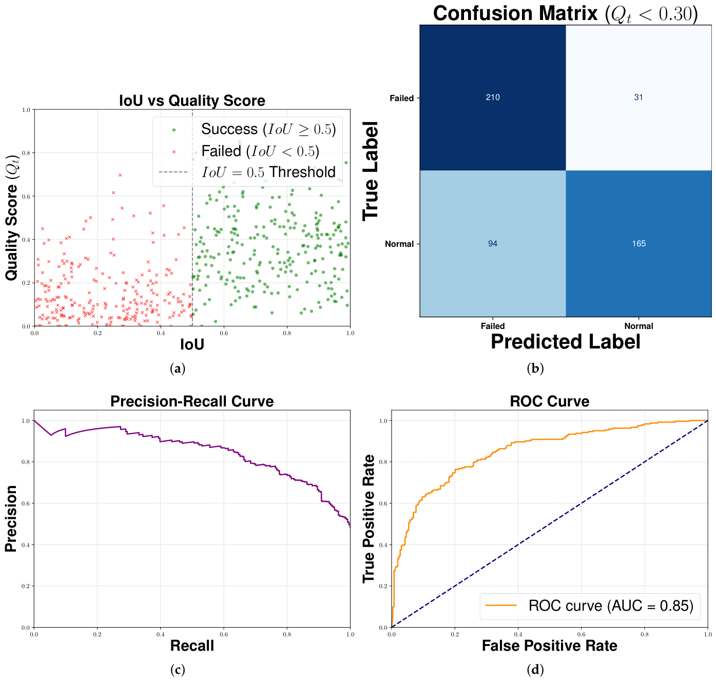
To evaluate the effectiveness of our quality metric Q t in detecting tracking failures, we treat tracking failure as the positive class and tracking success as the negative class. The evaluation results are summarized in Figure 16. First, we randomly sampled a number of frames from the tracking results as test samples. A tracking failure (positive sample) was defined as having an IoU below 0.5. All samples are plotted in Figure 16a. Let τ be the quality threshold. The prediction is classified as positive if Q t < τ . When τ = 0.3 , the corresponding confusion matrix shown in Figure 16b was obtained.
By varying τ , we generated the Precision-Recall (PR) curve in Figure 16c and the Receiver Operating Characteristic (ROC) curve in Figure 16d. The results demonstrate that our tracking quality score performance is satisfactory. It exhibits a high recall rate. Although the precision is relatively low, our objective is to identify tracking failures, which demands a higher recall rate. In practical tracking scenarios, we also sacrifice some precision to enhance recall. Therefore, this metric meets our requirements.

4.4. Long-Term Tracking on Embedded Device

Long-Term Tracking aims to stably track targets over video sequences spanning thousands of frames. Such sequences often involve various disturbances and better reflect real-world embedded tracking scenarios. Therefore, we evaluated the performance of HCLT in long-term tracking on embedded devices. For comparison, we selected classic Siamese network trackers (SiamFC [42], SiamRPN, DaSiamRPN [15]) and lightweight trackers (LightTrack [18], NanoTrack [14]), all capable of stable operation on embedded platforms. The experiments were conducted on the VOT2018-LT and VOT2022-LT datasets.
We first initialized all trackers only at the first frame and tested their runtime speeds. As shown in Table 5, HCLT achieved a speed comparable to that of lightweight trackers. In particular, these lightweight trackers are based on meticulously designed models, while HCLT attained similar average speeds simply by combining two types of trackers. Furthermore, its speed can be further improved by adjusting the frequency of tracker usage, demonstrating its versatility and flexibility.
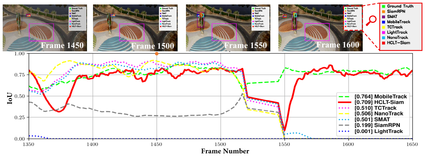
Visualization results of long-term tracking are presented in Figure 17. We selected a sequence with occlusions and plotted the corresponding IoU variation curve. As observed, only HCLT successfully recovered tracking after failure. This is because lightweight and classical models lack mechanisms to handle tracking failures, while most long-term optimized trackers introduce excessive computational overhead, making them unsuitable for embedded devices. We also counted the number of tracking failures across all sequences and found that HCLT significantly outperformed other trackers, confirming its robustness.
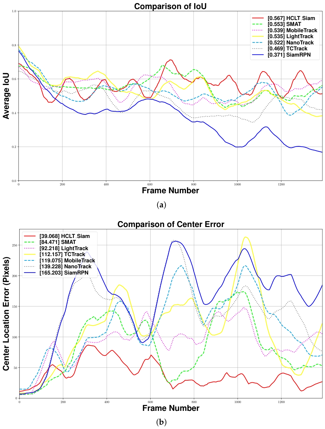
We further analyzed the performance of these trackers by incorporating re-initialization after tracking failures (i.e., when IoU drops to 0) to prevent error propagation from affecting the evaluation. By aggregating results from multiple sequences, we plotted the average IoU and average center error curves, as shown in Figure 18. HCLT demonstrated a clear advantage and exhibited satisfactory performance.

4.5. Real-Time Tracking on Embedded Device

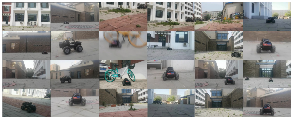
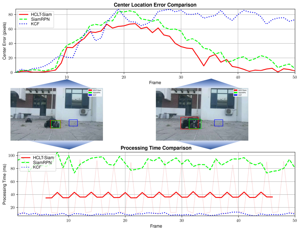
To evaluate the practical performance of HCLT, we conducted real-world object tracking using a camera on an embedded platform and analyzed the results. The images in Figure 19 illustrate video sequences captured during our tests. The camera generates a continuous image stream at a fixed rate, and we filter out severely blurred frames to prevent tracking degradation, though this may slightly affect the frame rate. After the operation, we manually annotated the target positions to calculate the center error of the tracking results, as shown in Figure 20.
The experiments adopt the HCLT-Siam tracker and compare it with SiamRPN and KCF. The experimental results demonstrate that HCLT-Siam can stably maintain a running speed of over 30 frames per second in real-time tracking, achieving a noticeable improvement compared with SiamRPN and fully meeting the real-time requirements of practical engineering applications. Meanwhile, HCLT-Siam achieves the lowest center error among the three trackers and exhibits excellent robustness in complex scenarios with multiple disturbance factors.

5. Discussion

5.1. Design Philosophy and Performance Analysis

HCLT draws inspiration from closed-loop control theory to address the problem of migrating high-computation deep trackers to resource-constrained embedded platforms while preserving robustness. The alternating detector scheme, combined with feedback–feedforward regulation, transforms the conventional open-loop TBD pipeline into a controllable closed-loop system.
The precision improvement stems from several interrelated factors. First, frame rate and accuracy are inherently coupled—higher frame rates preserve stronger inter-frame motion continuity, which benefits the matching process. Second, the quality scoring mechanism prevents single detection failures from cascading into permanent tracking loss, a common failure mode in open-loop TBD trackers. Third, although the feedforward and feedback channels do not individually produce large precision gains, their structural contributions are critical: the feedforward channel provides the primary signal for quality degradation detection, while the feedback channel stabilizes motion prediction across frames.
A closer examination reveals that the Kalman filter effectively functions as a temporal low-pass filter. The per-frame detector produces scale estimates containing high-frequency jitter caused by partial occlusions, motion blur, or background clutter. The Kalman prediction–update cycle attenuates these rapid fluctuations through its inherent state-measurement blending. An ablation study confirms this: enabling the TSO feedback reduces frame-to-frame scale jitter by 10–15% while center error and IoU remain effectively unchanged. The TSO thus serves as a defensive temporal regularizer that suppresses high-frequency scale noise without compromising responsiveness to genuine target changes.

5.2. Comparison with Existing Approaches

Existing multi-tracker methods typically combine multiple tracker outputs through result fusion or design plug-and-play performance enhancement modules. Both approaches increase per-frame computational load and are therefore unsuitable for resource-constrained embedded systems. HCLT avoids this problem by alternating between detectors rather than running them concurrently, which can even improve throughput relative to the heavier detector alone.
The handcrafted features in the feedforward channel and the Kalman filter in the feedback channel are deliberately simple. This simplicity is a design strength: they impose negligible computational overhead and integrate with any TBD-compatible deep tracker without modifying its internal end-to-end structure.

5.3. Applicable Scenarios and Limitations

The HCLT framework is best suited for long-term object tracking on edge-embedded devices, which match the requirements of industrial production monitoring, video surveillance, and similar real-world deployment scenarios.
Several limitations should be noted. First, the current work does not incorporate deep optimization targeting specific model architectures or hardware platforms; substantial headroom remains through model quantization or hardware-specific acceleration. Second, the framework introduces a relatively large number of tunable parameters, which increases deployment-time calibration complexity. Third, HCLT requires detectors that follow the TBD paradigm—trackers that maintain complex inter-frame temporal states cannot be directly integrated. Addressing these limitations will be the focus of future work.

6. Conclusions

We designed HCLT, a practical and flexible multi-tracker framework integrated with disturbance-resistance and recovery mechanisms. This approach effectively addresses the performance degradation that is often encountered in embedded computing due to limited computational resources and frequent environmental disturbances. Rather than solely pursuing SOTA precision metrics, HCLT prioritizes constructing a practical embedded tracking solution that optimizes the synergy between existing models and hardware constraints. Extensive experiments have comprehensively validated its effectiveness in multiple dimensions. Nevertheless, the current framework relies on the TBD paradigm; thus, the selection of trackers has limitations. Additionally, the precision of the current tracking quality estimation score remains suboptimal. Addressing these constraints and refining the quality evaluation metric will be the focal points of our future work.

Author Contributions

Conceptualization, X.W. and J.L.; methodology, J.L.; software, J.L.; validation, J.L., M.L.; formal analysis, J.L.; investigation, J.L.; resources, X.W.; data curation, J.L.; writing—original draft preparation, J.L.; writing—review and editing, X.W.; visualization, J.L.; supervision, X.W.; project administration, X.W.; funding acquisition, X.W. All authors have read and agreed to the published version of the manuscript.

Funding

This work was supported by the National Natural Science Foundation of China under Grant 62571367, 62271348, 62171312.

Data Availability Statement

Data are contained within the article.

Conflicts of Interest

The authors declare no conflicts of interest.

Abbreviations

The following abbreviations are used in this manuscript:
VOTVisual Object Tracking
SOTSingle Object Tracking
HCLTHybrid Closed-Loop Tracker
TBDTracking by Detection
CFCorrelation Filter
DLDeep Learning
TSOTracking State Observer
RDReliable Detector
FDFast Detector
FPSFrames Per Second
IoUIntersection over Union
AUCArea Under the Curve
EAOExpected Average Overlap

References

  1. Zhang, Z.; Wang, X.; Huang, D.; Fang, X.; Zhou, M.; Mi, B. iDT: An Integration of Detection and Tracking Toward Low-Observable Multipedestrian for Urban Autonomous Driving. IEEE Trans. Ind. Inform. 2023, 19, 9887–9897. [Google Scholar] [CrossRef]
  2. Chiu, Y.C.; Hsu, H.W.; Tsai, C.Y. Person Tracking Control of Mobile Robots Using a Lightweight Object Detection and Tracking System. In Proceedings of the 2024 8th International Conference on Robotics and Automation Sciences, Tokyo, Japan, 21–23 June 2024; pp. 21–25. [Google Scholar] [CrossRef]
  3. Cao, Z.; Li, J.; Shao, S.; Zhang, D.; Zhou, M. Siamese Adaptive Network-Based Accurate and Robust Visual Object Tracking Algorithm for Quadrupedal Robots. IEEE Trans. Cybern. 2025, 55, 1264–1276. [Google Scholar] [CrossRef] [PubMed]
  4. Sun, N.; Zhao, J.; Shi, Q.; Liu, C.; Liu, P. Moving Target Tracking by Unmanned Aerial Vehicle: A Survey and Taxonomy. IEEE Trans. Ind. Inform. 2024, 20, 7056–7068. [Google Scholar] [CrossRef]
  5. Li, Y.; Fu, C.; Ding, F.; Huang, Z.; Lu, G. AutoTrack: Towards High-Performance Visual Tracking for UAV with Automatic Spatio-Temporal Regularization. In Proceedings of the 2020 IEEE/CVF Conference on Computer Vision and Pattern Recognition (CVPR), Virtual, 14–19 June 2020; pp. 11920–11929. [Google Scholar] [CrossRef]
  6. Ge, Q.; Zhu, B.; Wang, M.; Zhang, B.; Huang, Y. Airborne Camera Dynamic Target Detection Based on Background Prediction and Semantic Compensation in Surface Environment. IEEE Trans. Circuits Syst. Video Technol. 2025, 35, 10973–10985. [Google Scholar] [CrossRef]
  7. Huang, K.; Zhang, Z.; Chen, J.; Kou, Y. A Survey of Single Object Tracking. In Proceedings of the 2025 6th International Conference on Electronic Communication and Artificial Intelligence (ICECAI), Chengdu, China, 20–22 June 2025; pp. 291–299. [Google Scholar] [CrossRef]
  8. Zhou, J.; Yao, Y.; Yang, R. Deep Learning for Single-object Tracking: A Survey. In Proceedings of the 2022 2nd IEEE International Conference on Software Engineering and Artificial Intelligence (SEAI 2022), Xiamen, China, 10–12 June 2022; pp. 12–19. [Google Scholar] [CrossRef]
  9. Yin, W.; Ye, Z.; Peng, Y.; Liu, W. A Review of Visible Single Target Tracking Based on Siamese Networks. In Proceedings of the 2023 4th International Conference on Electronic Communication and Artificial Intelligence (ICECAI 2023), Guangzhou, China, 12–14 May 2023; pp. 282–289. [Google Scholar] [CrossRef]
  10. Bolme, D.S.; Beveridge, J.R.; Draper, B.A.; Lui, Y.M. Visual Object Tracking Using Adaptive Correlation Filters. In Proceedings of the 2010 IEEE Computer Society Conference on Computer Vision and Pattern Recognition (CVPR), San Francisco, CA, USA, 13–18 June 2010; pp. 2544–2550. [Google Scholar] [CrossRef]
  11. Henriques, J.F.; Caseiro, R.; Martins, P.; Batista, J. High-Speed Tracking with Kernelized Correlation Filters. IEEE Trans. Pattern Anal. Mach. Intell. 2015, 37, 583–596. [Google Scholar] [CrossRef] [PubMed]
  12. Liang, Y.; Xiong, L.; Shan, Y.; Wang, H. Learning Multi-Task Target-Specific Correlation Filters for Robust Tracking. IEEE Trans. Circuits Syst. Video Technol. 2025, 35, 6698–6711. [Google Scholar] [CrossRef]
  13. Li, B.; Yan, J.; Wu, W.; Zhu, Z.; Hu, X. High Performance Visual Tracking with Siamese Region Proposal Network. In Proceedings of the 2018 IEEE/CVF Conference on Computer Vision and Pattern Recognition (CVPR), Salt Lake City, UT, USA, 18–22 June 2018; pp. 8971–8980. [Google Scholar]
  14. Chen, Z.; Zhong, B.; Li, G.; Zhang, S.; Ji, R.; Tang, Z.; Li, X. SiamBAN: Target-Aware Tracking with Siamese Box Adaptive Network. IEEE Trans. Pattern Anal. Mach. Intell. 2023, 45, 5158–5173. [Google Scholar] [CrossRef] [PubMed]
  15. Zhu, Z.; Wang, Q.; Li, B.; Wu, W.; Yan, J.; Hu, W. Distractor-Aware Siamese Networks for Visual Object Tracking. In Proceedings of the Computer Vision—ECCV 2018, Munich, Germany, 8–14 September 2018; pp. 103–119. [Google Scholar] [CrossRef]
  16. Bao, J.; Chen, K.; Sun, X.; Zhao, L.; Diao, W.; Yan, M. SiamTHN: Siamese Target Highlight Network for Visual Tracking. IEEE Trans. Circuits Syst. Video Technol. 2025, 35, 7061–7074. [Google Scholar] [CrossRef]
  17. Wang, J.; Chai, B.; Zhou, L.; Wang, Y. Robust Object Tracking via Long-Range Spatial Representation and Local Feature Enhancement. IEEE Trans. Circuits Syst. Video Technol. 2025, 35, 11362–11376. [Google Scholar] [CrossRef]
  18. Yan, B.; Peng, H.; Wu, K.; Wang, D.; Fu, J.; Lu, H. LightTrack: Finding Lightweight Neural Networks for Object Tracking via One-Shot Architecture Search. In Proceedings of the 2021 IEEE/CVF Conference on Computer Vision and Pattern Recognition (CVPR), Nashville, TN, USA, 19–25 June 2021; pp. 15175–15184. [Google Scholar] [CrossRef]
  19. Zhang, X.; Xu, H.; Yu, C.; Tan, G. PCTrack: Accurate Object Tracking for Live Video Analytics on Resource-Constrained Edge Devices. IEEE Trans. Circuits Syst. Video Technol. 2025, 35, 3969–3982. [Google Scholar] [CrossRef]
  20. Xu, Y.; Wang, Z.; Li, Z.; Yuan, Y.; Yu, G. SiamFC++: Towards Robust and Accurate Visual Tracking with Target Estimation Guidelines. Proc. AAAI Conf. Artif. Intell. 2020, 34, 12549–12556. [Google Scholar] [CrossRef]
  21. Choi, S.; Lee, J.; Lee, Y.; Hauptmann, A. Robust Long-Term Object Tracking via Improved Discriminative Model Prediction. In Proceedings of the Computer Vision—ECCV 2020 Workshops; Bartoli, A., Fusiello, A., Eds.; Springer: Cham, Switzerland, 2020; pp. 602–617. [Google Scholar] [CrossRef]
  22. Ma, C.; Yang, X.; Zhang, C.; Yang, M.H. Long-Term Correlation Tracking. In Proceedings of the 2015 IEEE Conference on Computer Vision and Pattern Recognition (CVPR), Boston, MA, USA, 7–12 June 2015; pp. 5388–5396. [Google Scholar] [CrossRef]
  23. Huang, L.; Zhao, X.; Huang, K. GlobalTrack: A Simple and Strong Baseline for Long-Term Tracking. Proc. AAAI Conf. Artif. Intell. 2020, 34, 11037–11044. [Google Scholar] [CrossRef]
  24. Bailer, C.; Stricker, D. Tracker Fusion on VOT Challenge: How Does It Perform and What Can We Learn about Single Trackers? In Proceedings of the 2015 IEEE International Conference on Computer Vision Workshops (ICCVW), Santiago, Chile, 7–13 December 2015; pp. 630–638. [Google Scholar] [CrossRef]
  25. Bailer, C.; Pagani, A.; Stricker, D. A Superior Tracking Approach: Building a Strong Tracker through Fusion. In Proceedings of the Computer Vision—ECCV 2014, Zurich, Switzerland, 6–12 September 2014; pp. 170–185. [Google Scholar] [CrossRef]
  26. Fan, H.; Ling, H. Parallel Tracking and Verifying: A Framework for Real-Time and High Accuracy Visual Tracking. In Proceedings of the 2017 IEEE International Conference on Computer Vision (ICCV), Venice, Italy, 22–29 October 2017; pp. 5487–5495. [Google Scholar] [CrossRef]
  27. Dunnhofer, M.; Micheloni, C. CoCoLoT: Combining Complementary Trackers in Long-Term Visual Tracking. In Proceedings of the 2022 26th International Conference on Pattern Recognition (ICPR 2022), Montréal, QC, Canada, 21–25 August 2022; pp. 5132–5139. [Google Scholar] [CrossRef]
  28. Rosten, E.; Drummond, T. Machine Learning for High-Speed Corner Detection. In Proceedings of the Computer Vision—ECCV 2006, Graz, Austria, 7–13 May 2006; pp. 430–443. [Google Scholar] [CrossRef]
  29. Lucas, B.D.; Kanade, T. An Iterative Image Registration Technique with an Application to Stereo Vision. In Proceedings of the 7th International Joint Conference on Artificial Intelligence (IJCAI), Vancouver, BC, Canada, 24–28 August 1981; Morgan Kaufmann Publishers Inc.: San Francisco, CA, USA; pp. 674–679. [Google Scholar]
  30. Kalman, R.E. A New Approach to Linear Filtering and Prediction Problems. J. Fluids Eng. 1960, 82, 35–45. [Google Scholar] [CrossRef]
  31. Zhang, Y.; Sun, P.; Jiang, Y.; Yu, D.; Weng, F.; Yuan, Z.; Luo, P.; Liu, W.; Wang, X. ByteTrack: Multi-object Tracking by Associating Every Detection Box. In Proceedings of the Computer Vision—ECCV 2022, Tel Aviv, Israel, 23–27 October 2022; pp. 1–21. [Google Scholar] [CrossRef]
  32. Le, X.; Gonzalez, R. Hybrid Salient Motion Detection Using Temporal Differencing and Kalman Filter Tracking with Non-Stationary Camera. In Proceedings of the 2017 IEEE International Conference on Image Processing (ICIP), Beijing, China, 17–20 September 2017; pp. 3345–3349. [Google Scholar] [CrossRef]
  33. Zhang, Z. A Flexible New Technique for Camera Calibration. IEEE Trans. Pattern Anal. Mach. Intell. 2000, 22, 1330–1334. [Google Scholar] [CrossRef]
  34. Ye, B.; Chang, H.; Ma, B.; Shan, S.; Chen, X. Joint Feature Learning and Relation Modeling for Tracking: A One-Stream Framework. In Proceedings of the Computer Vision—ECCV 2022, Tel Aviv, Israel, 23–27 October 2022; pp. 341–357. [Google Scholar] [CrossRef]
  35. Krizhevsky, A.; Sutskever, I.; Hinton, G.E. ImageNet Classification with Deep Convolutional Neural Networks. Commun. ACM 2017, 60, 84–90. [Google Scholar] [CrossRef]
  36. Wu, Y.; Lim, J.; Yang, M.H. Object Tracking Benchmark. IEEE Trans. Pattern Anal. Mach. Intell. 2015, 37, 1834–1848. [Google Scholar] [CrossRef] [PubMed]
  37. Kristan, M.; Leonardis, A.; Matas, J.; Felsberg, M.; Pflugfelder, R.; Kämäräinen, J.K.; Chang, H.J.; Danelljan, M.; Zajc, L.Č.; Lukežič, A.; et al. The Tenth Visual Object Tracking VOT2022 Challenge Results. In Proceedings of the Computer Vision—ECCV 2022, Tel Aviv, Israel, 23–27 October 2022; pp. 431–460. [Google Scholar] [CrossRef]
  38. Gopal, G.Y.; Amer, M.A. Separable Self and Mixed Attention Transformers for Efficient Object Tracking. In Proceedings of the 2024 IEEE/CVF Winter Conference on Applications of Computer Vision (WACV), Waikoloa, HI, USA, 3–8 January 2024; pp. 6708–6717. [Google Scholar]
  39. Cao, Z.; Huang, Z.; Pan, L.; Zhang, S.; Liu, Z.; Fu, C. TCTrack: Temporal Contexts for Aerial Tracking. In Proceedings of the 2022 IEEE/CVF Conference on Computer Vision and Pattern Recognition (CVPR), New Orleans, LA, USA, 19–24 June 2022; pp. 14778–14788. [Google Scholar] [CrossRef]
  40. Zhai, J.; Cheng, Z.; Zhang, W.; Zhu, D.; Yang, W. Efficient Object Tracking on Edge Devices with MobileTrack. J. Vis. Commun. Image Represent. 2024, 100, 104126. [Google Scholar] [CrossRef]
  41. Kristan, M.; Leonardis, A.; Matas, J.; Felsberg, M.; Pflugfelder, R.; Čehovin Zajc, L.; Vojir, T.; Bhat, G.; Lukezic, A.; Eldesokey, A.; et al. The Sixth Visual Object Tracking VOT2018 Challenge Results. In Proceedings of the Computer Vision—ECCV 2018, Munich, Germany, 8–14 September 2018; pp. 3–53. [Google Scholar] [CrossRef]
  42. Cen, M.; Jung, C. Fully Convolutional Siamese Fusion Networks for Object Tracking. In Proceedings of the 2018 25th IEEE International Conference on Image Processing (ICIP), Athens, Greece, 7–10 October 2018; pp. 3718–3722. [Google Scholar] [CrossRef]
Figure 1. The framework of HCLT. By alternating between two trackers to complete the tracking process, it enables dynamic adjustment of computational load. Additionally, an observation-feedback-recovery channel is designed to further enhance the robustness of HCLT in real-world tracking tasks. Alternating execution is the main working mode in the tracking process, while Observe and Recover are external methods. Solid arrows denote the main task loop, and dashed arrows denote condition-triggered branch tasks.
Electronics 15 02276 g001
Figure 2. HCLT’s framework, along with its comparison against single-detection tracking approaches, demonstrates a significant improvement in processing efficiency. Within the same time interval, HCLT is capable of handling a markedly greater number of frames. Blue indicates the single-detection working mode, and green indicates HCLT’s hybrid-detection working mode. The dashed Recover arrow indicates that the recovery process is used only when the target is judged to be lost.
Electronics 15 02276 g002
Figure 3. The workflow of HCLT mainly consists of four steps and can run across three distinct processes to enhance the tracking of real-time performance. Red arrows indicate the feedback process, and purple arrows indicate the feedforward process.
Electronics 15 02276 g003
Figure 4. Coordinate transformation and image-plane projection under camera motion. Camera motion may change the projected position of the target in the image plane and affect tracking; therefore, TSO considers such projection variations. Solid lines denote the coordinate axes, image plane, and target projection, while dashed lines indicate auxiliary projection rays and reference planes.
Electronics 15 02276 g004
Figure 5. The feedforward channel operates only on the current frame, while the feedback channel acts on the next frame. Spatial information adjusts the current state through the feedforward channel, and the current state acts on the search region of the next frame via the feedback channel. Red arrows indicate the feedback process, and purple arrows indicate the feedforward process.
Electronics 15 02276 g005
Figure 6. Visualization of intermediate results during the tracking process. Incorporating velocity observations and feature points can enhance the accuracy and stability of tracking.
Electronics 15 02276 g006
Figure 7. Distracted search alters the traditional search strategy by utilizing velocity information to derive a new search region after tracking failure, thereby enabling tracking recovery. Blue dots denote incorrect target predictions, and red dots denote the true target positions.
Electronics 15 02276 g007
Figure 8. Each step of temporally continuous search crops the search region on a new frame, while spatial expansion search crops the search region at different positions within the same frame, thereby reducing the computational burden associated with extensive searches required for tracking recovery. Arrows indicate temporal changes, yellow dots denote historical target positions, red dots denote the true target positions, blue dashed boxes indicate search ranges, and shaded boxes indicate the actual search regions. (a) Temporally continuous search. (b) Spatial expansion search.
Electronics 15 02276 g008
Figure 9. Embedded hardware platform and several key components. The camera is equipped with steerable servos for object tracking or introducing motion disturbance.
Electronics 15 02276 g009
Figure 10. Success plot and precision plot of OTB2015 with recently lightweight trackers. One-Pass Evaluation (OPE) refers to annotating targets only on the first frame. (a) Success plot. (b) Precision plot.
Electronics 15 02276 g010
Figure 11. Precision–recall curve on VOT2018-LT dataset. Curves closer to the top-right corner indicate better long-term tracking performance. Dots on the curves denote the maximum F1-score points.
Electronics 15 02276 g011
Figure 12. Visual effects of four representative disturbances.
Electronics 15 02276 g012
Figure 13. The accuracy of the tracker is evaluated using the logarithm of the mean center error, while its speed is assessed based on the average FPS. Trackers positioned closer to the top-right corner exhibit superior performance. The blue dashed line and red solid line are used only for a simple comparison of variation trends and have no actual meaning under the logarithmic coordinate.
Electronics 15 02276 g013
Figure 14. The performance was evaluated on the same video sequences, using the same success rate and precision metrics as defined in the OTB2015 benchmark. (a) Success plot. (b) Precision plot.
Electronics 15 02276 g014
Figure 15. Judgment of tracking failure caused by different disturbances based on quality score.
Electronics 15 02276 g015
Figure 16. The evaluation metrics for some classifiers. (a) A scatter plot obtained from random sampling of video frames. Tracking is considered a failure when Intersection over Union (IoU) < 0.5 . (b) A confusion matrix of the true tracking state versus the predicted tracking state for randomly sampled instances, with tracking failure defined as the positive class. (c) A PR curve for quality estimation. (d) A ROC curve for quality estimation.
Electronics 15 02276 g016
Figure 17. The tracker outputs bounding boxes along with the corresponding IoU curves for these frames. The curves have been smoothed.
Electronics 15 02276 g017
Figure 18. (a) Average IoU across multiple video sequences. (b) Average center error across multiple video sequences. The curves have been smoothed.
Electronics 15 02276 g018
Figure 19. The video sequence obtained through real-time detection. The scene contains multiple types of disturbances.
Electronics 15 02276 g019
Figure 20. The center error and processing time for each frame in the video sequence. The red dashed line represents the actual processing time, while the red solid line denotes the smoothed average processing time.
Electronics 15 02276 g020
Table 1. Parameter initialization of the HCLT framework. Parameters are grouped by functional component.
ParameterValueDescription
Quality Estimation
    β 0.80EMA smoothing coefficient
    θ p 0.6Detector response normalization constant
    λ 0.5Feature retention penalty strength
   K15Sliding window length for M a v g
    τ 10Look-back offset for feature retention change Δ r f
   Warmup frames20Frames before quality evaluation activates
Hysteresis State Machine
    θ b a d 0.30Instantaneous quality threshold for “bad” frame
    θ g o o d 0.50Instantaneous quality threshold for “good” frame
    N b a d 8Consecutive bad frames to enter LOST
    M g o o d 3Consecutive good frames to exit LOST
Quality-Gated Detector Switching
    τ l o w 0.40Suppress FD when Q t drops below
    τ h i g h 0.65Resume FD when Q t recovers above
    f t a r g e t 30–60Target frame rate (FPS) for speed-aware interleaving
Feature Tracker (Feedforward)
    M m a x 30Maximum feature points
    M m i n 5Minimum feature points for offset correction
    w L K 15 × 15Lucas–Kanade window size
    η 0.15Feedforward correction weight
Table 3. Precision, recall, and F1-score on VOT2018-LT. Trackers are ranked by F1-score in descending order.
TrackerPrecisionRecallF1
HCLT-OS0.7020.6770.689
OSTrack0.6760.6680.672
SMAT0.6940.5830.634
LightTrack0.6080.4790.536
HCLT-Siam0.6200.4540.525
NanoTrack0.6770.4070.509
TCTrack0.6280.4140.499
MobileTrack0.6560.3880.488
SiamRPN0.5390.3160.398
Table 4. Performance comparison between baseline trackers and the proposed Hybrid framework. All tests are conducted on the CPU. The FD in all Hybrid Framework entries is KCF; therefore, the KCF row is marked with “—” because its hybrid result is already represented as the common FD.
TrackersBaseHybrid Framework
SuccPrecFPSAUCPreFPS
OSTrack0.6780.89070.6720.88532
DaSiamRPN0.6580.880130.6650.88143
SiamRPN0.6290.847110.6420.86141
SiamFC0.5860.772280.6010.81263
KCF0.5780.783407
Table 5. FPS comparison between HCLT and other trackers. The video resolution is 720p.
TrackerFPS
HCLT39
NanoTrack>60
LightTrack33
TCTrack40
SMAT45
MobileTrack22
SiamRPN9
Disclaimer/Publisher’s Note: The statements, opinions and data contained in all publications are solely those of the individual author(s) and contributor(s) and not of MDPI and/or the editor(s). MDPI and/or the editor(s) disclaim responsibility for any injury to people or property resulting from any ideas, methods, instructions or products referred to in the content.