Article

LGP-Net: A Lightweight Gated-Fusion Network with Physics-Informed Features for Automatic Modulation Classification


1
The College of Electronic Information and Optical Engineering, Nankai University, Tianjin 300350, China
2
Tianjin Key Laboratory of Optoelectronic Sensor and Sensing Network Technology, Nankai University, Tianjin 300350, China
*
Author to whom correspondence should be addressed.
Electronics 2026, 15(11), 2261; https://doi.org/10.3390/electronics15112261
Submission received: 26 April 2026 / Revised: 18 May 2026 / Accepted: 21 May 2026 / Published: 23 May 2026

Abstract

The growing diversity of wireless standards and complex real-world channel effects render automatic modulation classification (AMC) increasingly challenging for spectrum monitoring and edge intelligence. However, most competitive deep-learning-based AMC networks still require 10 5 10 6 parameters, exceeding the memory available on resource-constrained edge platforms. We propose LGP-Net, a lightweight gated-fusion network that pairs a physics-informed expert branch with a compact temporal encoder built from depthwise separable convolution (DSConv), squeeze-and-excitation (SE) attention, and a single-layer gated recurrent unit (GRU). Specifically, unlike other dual-branch structures that directly concatenate the outputs of both pathways, this work designs a lightweight gating unit that requires no external signal-to-noise ratio (SNR) labels and adaptively reweights the two pathways according to signal-quality degradation. With fewer than 40 K parameters, a peak activation footprint of 26.00 KB and an amortised inference latency of 9.7 μ s per sample under GPU acceleration, LGP-Net attains 65.00% overall accuracy on RadioML 2016.10B (91.48% at 0 dB) and 62.76% on RadioML 2016.10A, placing it in a competitive accuracy–efficiency regime relative to architectures consuming 5× to 500× more parameters. These characteristics support deployment-oriented feasibility under memory-constrained edge settings and high-throughput spectrum-monitoring pipelines.

1. Introduction

Automatic modulation classification (AMC) identifies the modulation scheme of an incoming radio signal without prior knowledge of its transmission parameters. It underpins cognitive radio, electronic surveillance, and adaptive receiver design, and its relevance has grown sharply with spectrum densification. Internet-of-Things devices, unmanned aerial vehicles, and 6G-oriented systems now share increasingly crowded bands, making accurate modulation recognition under tight computational budgets and noisy channel conditions a practical requirement. Two recent surveys [1,2] converge on the same diagnosis: the complexity–accuracy trade-off, low-SNR robustness, and real-time edge deployment remain persistent open problems in the field.
AMC research has long been organised around two paradigms [1]. The first is likelihood-based hypothesis testing, which is asymptotically optimal in theory. In practice, however, it demands precise knowledge of the channel model and can make real-time operation difficult on resource-constrained platforms. The second paradigm extracts hand-crafted statistical descriptors, such as higher-order cumulants [3], amplitude histograms, and phase-difference moments, and feeds them to a shallow classifier such as a support vector machine or decision tree. Recognition accuracy under this pipeline is dictated largely by whether the selected statistics remain informative when the operating environment shifts.
Since the release of the RadioML benchmark datasets, these two paradigms have been increasingly complemented, and often surpassed, by deep learning approaches [4], which we review in the context of recent lightweight and fusion-oriented designs.
Despite remarkable advances in automatic modulation classification (AMC) [4,5] driven by deep learning in recent years, practical edge-oriented AMC still faces three coupled requirements. First, high-performing deep AMC models [1,2], as catalogued in the related work section below, often rely on parameter counts in the 10 5 10 6 range [6], which can exceed the on-chip static random-access memory (SRAM) capacity of many microcontrollers and small software-defined radio (SDR)/field-programmable gate array (FPGA) platforms. Second, aggressive architectural compression can reduce the redundancy needed to separate modulation patterns at low signal-to-noise ratio (SNR), where waveform-level cues are strongly corrupted. Third, when heterogeneous signal cues are available, fixed or coarse feature aggregation cannot adjust the branch balance for each degraded sample.
These observations motivate a model that is compact, noise-aware, and adaptive at inference time. LGP-Net therefore combines a data-driven temporal encoder with a physics-informed expert branch, and balances the two pathways through lightweight per-dimension gates trained without explicit SNR supervision.
Our main contributions can be summarised as follows:
1.
We design LGP-Net as two complementary branches. The temporal branch uses depthwise separable convolution (DSConv) with squeeze-and-excitation (SE) attention followed by a single-layer gated recurrent unit (GRU) to extract waveform-level representations from in-phase/quadrature (IQ)-derived inputs. The expert branch encodes 11 domain-specific signal statistics that provide noise-averaging cues less sensitive to sample-level fluctuations. By merging these complementary representations, the model jointly exploits learned temporal structure and analytically grounded statistical priors.
2.
LGP-Net employs a per-dimension sigmoid gate to address adaptive fusion without explicit SNR labels. Unlike fusion strategies with fixed or globally shared weights, this gate is a lightweight linear layer trained solely on the classification loss. This per-sample, per-dimension routing adjusts the temporal–expert balance without introducing a separate SNR-estimation module in the inference pipeline.
3.
We establish LGP-Net as a compact, accuracy-oriented operating point for lightweight AMC rather than a model that merely minimises parameter count. Under identical evaluation protocols, it achieves 65.00% accuracy on RadioML 2016.10B and 62.76% on RadioML 2016.10A with fewer than 40 K parameters, a peak activation memory of 26.00 KB, and dynamic 8-bit integer (INT8) post-training quantisation that preserves recognition accuracy while reducing the serialised state size by about 53%. These results provide a unified accuracy–efficiency reference for future lightweight AMC comparisons under RadioML-based evaluation.
The remainder of this paper is organised as follows. Section 2 surveys related work on AMC. Section 3 describes the network architecture and computational complexity. Section 4 details the dataset and training protocol. Section 5 reports classification results, lightweight-baseline comparisons, deployment-oriented feasibility analysis, ablation studies, robustness tests, and gate-behaviour analysis. Section 6 summarises the findings and future directions.

2. Related Work

This section reviews representative work on deep-learning-based modulation recognition architectures, lightweight AMC models, and multi-cue fusion with knowledge-driven schemes.

2.1. Preliminary Architectures Derived from Deep Learning

The release of the RadioML benchmark datasets catalysed the shift toward data-driven AMC. Early work [4] showed that even a two-layer convolutional network trained directly on raw in-phase/quadrature (IQ) samples could match or surpass traditional classifiers. Deeper residual and hybrid CNN–recurrent [5] architectures subsequently raised the accuracy bar. Later contributions explored LSTM-based denoising autoencoders [6], attention-enhanced recurrent models [7], and CNN-GRU hybrids [8].
Transformer-based designs have likewise drawn considerable attention along this line. Cai et al. [9] ported the Transformer architecture to modulation-classification tasks, whereas Kong et al. [10] took a rather different route by wrapping a Transformer encoder inside a contrastive semi-supervised framework. Recent studies such as IQFormer [11], SMTrans [12], and the MFCA-Transformer [13] continued this direction by exploring different tokenisation schemes or fusion strategies on top of a Transformer backbone. However, these Transformer-oriented designs are not primarily optimised for the compact edge-oriented regime considered here because accuracy improvements built upon mainstream Transformer architectures generally entail non-negligible parameter overhead.

2.2. Lightweight AMC Architectures

Compression of AMC networks for edge deployment has become a research direction in its own right. Guo et al. [14] proposed ULCNN, which combines complex-valued convolution with channel shuffling in only 9751 parameters and runs in real time on a Raspberry Pi 4B; its absolute accuracy, however, is substantially lower than that of mid-sized models. Huo et al. [12] introduced SMTrans, a scale-aware modulation Transformer that reaches 63.27% accuracy with roughly five times fewer parameters and fifteen times fewer FLOPs than comparable Transformer designs.
Other efficient baselines include MCLDNN [15] and MCNet [16]. PET-CGDNN [17] further showed that lightweight modulation recognition can be maintained with around 70 K parameters through parameter estimation and transformation, whereas SCNN [18] explored a decentralised-learning-based lightweight design. Ke and Vikalo’s LSTM Auto-Encoder/DAE [6] is also worth noting: with only about 15 K parameters, it coupled recurrent sequence encoding with reconstruction-assisted learning and achieved highly competitive performance at the time, providing an instructive lightweight reference for later compact AMC designs.
Kong et al. [19] reported in 2025 that a TCN–Mamba fusion architecture delivers up to a 3.8 dB SNR gain at 90% accuracy while keeping the parameter count and inference latency low. Its model size, however, still exceeds the compact regime targeted in this work, and the reported 59.12% average accuracy leaves headroom for improvement.
Robustness at low SNR remains a central difficulty. Lin et al. [7] applied signal-enhancement preprocessing and found that it attenuates noise corruption to a degree, yet accuracy still collapses once SNR falls below roughly 0 dB. The failure mechanism is informative: convolutional and recurrent layers operate on each local window under translation-invariant kernels, so when the noise power exceeds the signal power, the filters may respond to stochastic fluctuations rather than modulation-specific structure—the network is not simply uncertain but may fit noise-driven local fluctuations.
Suman et al. [20] proposed DP–DRSN, a dual-path deep residual shrinkage network that embeds garrote denoising in the forward pass. With 27 K parameters, it has a reported accuracy of 61.20% on RadioML 2016.10A, suggesting that a noise-aware prior can benefit lightweight AMC. However, this accuracy remains near the apparent raw-IQ plateau, which motivates supplementing architectural compression and implicit denoising with noise-robust statistical descriptors.
The Mamba architecture, built on selective state-space models, has also entered the AMC arena: MAMCA [21] is the first Mamba-based AMC backbone and offers favourable GPU memory and latency characteristics for long signal sequences. Related efforts include lightweight TCN–GRU hybrids [22], knowledge distillation from heavy DRSN teachers to compact ShuffleNetV2 students [23], the multi-level distillation network MLD-Net [24] that transfers Transformer knowledge to a Reformer-based student at three granularity levels, and the progressive differentiable architecture search of Zhang et al. [25].
A common thread runs through this body of work: the resulting models rely exclusively on features learned from raw IQ waveforms. Their accuracy on RadioML 2016.10A has largely converged to around 62%, while the corresponding value on RadioML 2016.10B is about 63% [20]—a plateau that appears difficult to break by purely architectural means. Further parameter reduction is therefore unlikely to yield meaningful accuracy gains unless additional inductive biases are introduced.

2.3. Multi-Cue Fusion and Knowledge-Driven AMC

A third strand of recent work fuses multiple views of the signal. Jiang et al. [26] proposed MAFFNet, a dual-branch ViT–LSTM architecture that combines raw IQ with amplitude/phase information through a learnable element-wise weighted module under an orthogonal-constraint loss, reaching 82.53% accuracy in the 0–10 dB range on RadioML 2018.01A. Shao et al. [11] proposed IQFormer, whose Dynamic Fusion Embedding module aggregates IQ and time–frequency features at the embedding stage. The MFCA-Transformer [13] fuses constellation diagrams, time–frequency maps, and power-spectrum features through a triple dynamic feature fusion module built on the Swin Transformer, reporting a high-SNR peak accuracy of 93.2% on RadioML 2016.10A. M-LSCANet [27] further shows a representative SNR-segmented use of time-domain and constellation-diagram branches: constellation information is exploited in medium- and high-SNR regions, whereas the constellation branch is disabled at low SNR because noise-blurred constellations may interfere with recognition. Lightweight realisations of multi-feature fusion based on asymmetric convolution blocks and hybrid channel attention have also been demonstrated [28].
A related line of work injects domain knowledge into the model itself. Zheng et al. [29] proposed the HKDD framework, which fuses higher-order cumulants and instantaneous statistics with CNN-learned IQ features through an attention mechanism. Ding et al. [30] described a data-and-knowledge dual-driven scheme aimed at 6G modulation classification. Li et al. [31] embedded modulation expertise into training through a knowledge graph and a feature aggregation loss. Zheng et al. [32] took a different route and injected prior knowledge through regularisation, an approach that operates on the loss surface rather than providing adaptive runtime fusion.
The fusion strategies surveyed above share a structural limitation: their fusion weights are either fixed hyperparameters or globally learned constants, neither of which tracks how the relative reliability of the two information sources changes with SNR. A recent attempt [33] introduces SNR as an explicit gating signal, but this design requires the noise level as an external input, which is rarely available at inference time. LGP-Net addresses this gap by inferring the noise regime from the signal itself, sample by sample and dimension by dimension, without requiring any external SNR estimate.

3. Proposed Method

3.1. Overview

LGP-Net uses a functional split among three lightweight components: a temporal branch extracts waveform-level features from a four-channel IQ-derived input, an expert branch encodes an 11-dimensional vector of physics-informed statistics, and a gated fusion unit determines how the two d-dimensional representations should be combined. The fused representation h fusion is passed to a single linear Classifier head at inference, while two auxiliary heads on h time and h expert are used only during training.
Figure 1 traces this data flow. A raw IQ segment is first augmented with instantaneous amplitude and phase channels and then processed by the temporal branch, where DSConv blocks with SE attention, a residual skip, and a single-layer GRU produce h time R d . In parallel, 11 physics-informed statistics are computed directly from the raw IQ samples and passed through a multilayer perceptron (MLP) with two layers to form h expert R d . A per-dimension sigmoid gate g combines the two representations into h fusion , which is then projected to class logits by the Classifier head.

3.2. Input Representation

Each received signal segment is represented as X IQ R 2 × 128 , containing 128 time-domain samples of the in-phase component I [ n ] and quadrature component Q [ n ] . Two derived channels, instantaneous amplitude A [ n ] and phase P [ n ] , are appended:
A [ n ] = I [ n ] 2 + Q [ n ] 2 , P [ n ] = atan 2 Q [ n ] , I [ n ] ,
producing a four-channel tensor X R 4 × 128 . Each channel is standardised independently per sample:
X c [ n ] X c [ n ] μ c σ c + ϵ 1 , c { I , Q , A , P } ,
where μ c and σ c are the mean and standard deviation of channel c computed along the time axis for the given sample, and ϵ 1 = 10 8 guards against division by zero. This standardisation removes sample-specific amplitude-scale variation before temporal encoding while preserving the waveform shape within each channel.
The normalised tensor X feeds only the temporal branch. By contrast, the expert features are extracted from the original complex baseband signal z [ n ] = I raw [ n ] + j Q raw [ n ] before any Z-score operation; otherwise, the power and amplitude-scale statistics would lose their physical meaning. The resulting 11-dimensional feature vector h prior R 11 is then globally Z-score normalised using the training-set mean and standard deviation before being passed to the expert branch MLP. Table 1 summarises the three normalisation stages used in the model.

3.3. Expert Branch and Physics-Informed Features

An 11-dimensional physics-informed feature vector forms the second information pathway in LGP-Net. These features target a well-known weakness of purely data-driven temporal models: noise-induced degradation below 0 dB SNR. By extracting analytically motivated statistics from raw IQ samples, the expert branch supplies discriminative information that is less sensitive to Gaussian noise than waveform-level representations, helping compensate for when learned filters struggle to infer modulation structure from severely corrupted signals.
A natural alternative would be to introduce a second deep branch over a frequency-domain, time–frequency, or constellation-image representation. We did not adopt this route because LGP-Net is designed to obtain a complementary information source under a strict lightweight budget and without external SNR labels, rather than simply increasing the number of learned encoders. The expert branch therefore deliberately uses aggregate physics-informed statistics whose noise-degradation behaviour differs from that of waveform-level temporal features.
Our design draws on the strengths of traditional methods [3]: rather than asking the network to rediscover these regularities at every training epoch, we endow the model with a structured prior that encodes the physical generation mechanism of each modulation family. This structured prior allows the temporal branch to focus on waveform-level temporal patterns.
Before presenting the feature definitions, we first establish the notational conventions used throughout this section. Table 2 summarises the key signal representations and derived quantities referenced in the sequel.
The 11 features are organised into three functionally complementary groups. Group 1 (G1, features 0–3) describes the power envelope and its fluctuations, which are most effective at separating constant-envelope modulations from amplitude-varying ones. Group 2 (G2, features 4–6) captures phase dynamics and instantaneous-frequency behaviour, discriminating frequency- and phase-modulated formats. Group 3 (G3, features 7–10) consists of higher-order cumulants, whose values are theoretically distinct across standard modulation families such as PSK, QAM and PAM [3]. Table 3 lists the complete set of definitions.
We adopt and combine these features because each group captures a different aspect of the signal. No single group is sufficient for robust recognition across the full 11-class set. Ablation experiments further confirm that the three feature groups contribute complementary discriminative power throughout the entire SNR range, with each encoding a distinct set of modulation-specific statistics. The downstream MLP learns nonlinear interactions among the statistics exploited by each modulation family, rather than treating them as mutually independent inputs.
As established in Swami and Sadler [3], this property is important in the low-SNR regime: every feature in Table 3 is an aggregate statistic computed over the full 128-sample window. Aggregation suppresses additive white Gaussian noise at a rate approximately proportional to 1 / N , so the expert feature vector degrades more gradually than the sample-wise representations used by the temporal branch. The fourth-order cumulants in G3 are particularly useful in this respect because their aggregate form averages out zero-mean noise while preserving modulation-specific structure. As a result, the expert branch can exploit this noise-suppression property with minimal parameter overhead to strengthen lightweight recognition.
We summarise the resulting 11-dimensional raw feature vector h prior R 11 . Before being fed into the expert branch MLP, it is first globally Z-score normalised using the training-set mean and standard deviation. The normalised expert vector h prior R 11 is encoded by a two-layer MLP:
h expert = LN GELU W 2 GELU ( W 1 h prior ) R d ,
where W 1 R 144 × 11 , W 2 R d × 144 , dropout with p = 0.1 is applied between the two layers (after the first GELU), and LN denotes layer normalisation applied to the output of the second GELU.
The hidden dimension of 144 was selected during preliminary architecture tuning: smaller values (≤64) limited the expressive capacity of the first layer and reduced validation accuracy, whereas larger values (≥256) increased the expert-branch parameter count beyond 15,000 without measurable performance improvement, thereby moving away from the lightweight intent of the expert pathway.
The final layer normalisation aligns the amplitude scale of the expert and temporal features, supporting stable operation of the subsequent gated fusion process. This lightweight feature representation serves as a noise-aware complement to the richer but more noise-sensitive features summarised by the temporal branch.

3.4. Temporal Branch

The expert vector is a physics-based summary, but relying solely on expert features can reproduce a limitation of traditional methods: insufficient information capture. Modulation schemes also leave subtler fingerprints, such as brief phase excursions, instantaneous envelope asymmetry, and sample-trajectory aggregation patterns that depend on modulation order. These cues cannot be fully captured by any predefined fixed statistical metric.
Therefore, a learnable pathway that operates directly on the waveform remains necessary. Existing methods along this direction often require large parameter budgets for modest accuracy gains. In our design, the physics-informed expert branch reduces the burden on the learned temporal pathway, allowing the model to remain compact while retaining competitive accuracy.

3.4.1. Depthwise Separable Convolution with SE Attention

Following Xception [34], we replace standard 1-D convolution with depthwise separable convolution. A standard conv uses C in · C out · k weights. The factorisation separates spatial filtering from channel mixing, which together total C in ( k + C out ) . For our first block ( C in = 4 , C out = 20 , k = 7 ), this reduces the parameter count by approximately 81%. The saving grows further in deeper blocks as C out increases. Meanwhile, the kernel span and channel-mixing capacity are preserved, so the accuracy cost of the factorisation is negligible. Each block is defined as
DSConv ( x ) = GELU BN PW DW ( x ) ,
with depthwise convolution DW , pointwise mixing PW , batch normalisation BN , and GELU activation on the main pathway.
The stack uses channel counts 4 20 48 d and kernel sizes 7 5 3 . Shallow layers require a larger temporal window to cover a full symbol cycle, but the corresponding feature types, such as symbol-rate periodicity and coarse envelope variation, are relatively limited, so a moderate channel count is sufficient. Deeper layers model shorter-range variations, where more short kernels are preferable to a small number of long kernels. This configuration of decreasing kernel size and increasing channel count is common in lightweight one-dimensional convolutional front ends.
Squeeze-and-excitation modules [35] are attached to the first two DSConv blocks. Each SE unit averages every channel over time and passes the resulting descriptor through a two-layer bottleneck MLP to obtain a per-channel weight:
s = σ W 4 ReLU ( W 3 GAP ( x ) ) , x ^ = x s ,
where GAP is temporal average pooling, W 3 R ( C / r ) × C and W 4 R C × ( C / r ) form the bottleneck at reduction ratio r = 8 , and σ is the sigmoid.
The output s [ 0 , 1 ] C reweights each channel: noise-dominated channels are suppressed, whereas informative channels are amplified. We use ReLU inside the SE bottleneck because its output is expected to approach a hard on/off pattern, while the main pathway retains GELU for smoother gradient flow.
A 1 × 1 projection connects the first DSConv block to the third, bridging the channel gap:
x 3 = DSConv 3 DSConv 2 ( x 1 ) + Proj 1 × 1 ( x 1 ) .
We chose the block-1 anchor rather than block-2 because the 20 d width change between block 1 and block 3 is much larger than the 48 d change between block 2 and block 3. Shortcuts across larger representation changes tend to carry more low-level information that two successive nonlinearities would otherwise erase. This information includes coarse envelope structure, which helps distinguish AM-DSB from WBFM, and low-frequency phase trends relevant to QPSK versus 8PSK. The shortcut also assists gradient flow during training.

3.4.2. Sequential Memory via GRU

The feature map x 3 R d × 128 is transposed to ( 128 , d ) and read by a single-layer GRU [36]; the hidden state at the final time step forms the branch output:
h time = GRU x 3 R d .
The convolutional operations, regardless of their depth, process each local window under the principle of translation invariance and are therefore incapable of representing the sequential relationships between events.
However, temporal order is crucial for several modulation types, including CPFSK frequency sweeps and QPSK phase transitions. Similar instantaneous phase jumps can carry different meanings depending on their ordering. The GRU at the end of the temporal branch supplies this sequential memory capacity.

3.5. Gated Fusion Unit

At this stage, the network contains two d-dimensional representations of the same signal. The first, h time , is a learned description extracted by the temporal branch; it captures rich, data-driven patterns but inherits the noise present in the underlying waveform. The second, h expert , summarises the signal with analytically selected statistics that average over the full observation window and therefore degrade more gradually as noise power increases.
The extent to which each description should be trusted depends on the instantaneous noise regime, which varies not only across samples but also across representation dimensions within a single sample. A fixed weighting scheme cannot track this variation; it imposes a ratio calibrated for one SNR regime and becomes suboptimal elsewhere. The gated fusion unit is designed to address this problem by operating at the granularity of individual dimensions and individual samples, assigning a separate trust coefficient to each element of the two d-vectors.
Concretely, the two branch outputs are concatenated along the channel axis and projected through a single linear layer followed by an element-wise sigmoid to yield the gate vector g . The fused representation is then formed as a convex combination:
g = σ W g [ h time h expert ] + b g [ 0 , 1 ] d ,
h fusion = g h time + ( 1 g ) h expert .
Here W g R d × 2 d and b g R d are the only trainable parameters; [ · · ] denotes concatenation and ⊙ the Hadamard product.
Because W g receives both branch outputs jointly, it can compare the statistical signatures of the two representations: a clean, well-organised h time differs markedly from one dominated by noise. The expert vector, composed of cumulants and envelope moments, retains a degree of discriminative power across SNR regimes. The linear layer then compares the two signatures and estimates which side is more trustworthy along each dimension. A value g k close to one favours the temporal description along dimension k, whereas a value close to zero favours the expert description along the same dimension.

3.6. Classification Heads and Multi-Task Loss

For final classification, the fused representation h fusion is mapped to the C candidate modulation classes by a single linear head, which is the only classifier retained at inference:
y ^ final = W f Dropout 0.3 ( h fusion ) .
Two additional linear heads are attached during training, one directly on h time and another on h expert :
y ^ time = W t h time , y ^ expert = W e h expert ,
where W { f , t , e } R C × d . The auxiliary heads are included to prevent a branch-starvation failure mode observed in preliminary runs with a single fused head. Once the gate begins to favour one branch during training, the other branch receives weaker gradients; its features then drift, its contribution to the fused representation becomes progressively less informative, and the gate learns to rely on it even less. This feedback loop is difficult to escape without additional supervision. With auxiliary heads, each branch is trained to classify independently so that both h time and h expert receive a direct supervisory signal at every step regardless of how the gate currently weights them.
The training objective is a weighted sum of three focal-loss terms:
L = L focal ( y ^ final , y ) + 0.5 L focal ( y ^ time , y ) + 0.5 L focal ( y ^ expert , y ) ,
with unit weight on the fused head and weight 0.5 on each auxiliary head. Using 0.5 for each auxiliary term gave the best balance in validation tuning: noticeably smaller weights left the starved branch under-supervised, whereas noticeably larger weights pulled the two branches toward individual accuracy at the expense of joint complementarity.
We use focal loss [37] with a label-smoothed target:
L focal = c = 1 C y ˜ c ( 1 p c ) γ log p c ,
y ˜ c = 1 ϵ ls if c = y , ϵ ls / ( C 1 ) otherwise ,
with focusing parameter γ = 2.0 and smoothing strength ϵ ls = 0.1 . Here p c denotes the softmax probability assigned by the head to class c.
This formulation applies the focal weight ( 1 p c ) γ to every term of a label-smoothed cross-entropy, a mild variant of the original formulation of Lin et al. [37]; we found it simpler to implement and numerically stable in mixed precision. The two ingredients play complementary roles: the focal weight concentrates optimisation effort on examples the model currently misclassifies (low-SNR samples and perennially confused pairs such as QAM16/QAM64 and AM-DSB/WBFM), while label smoothing prevents the network from pushing p c arbitrarily close to one on any class, acting as an entropy regulariser that improves calibration.

3.7. Computational Complexity and Structural Parameterisation

Table 4 lists the layer-by-layer parameter and multiply-accumulate operation (MAC) breakdown of LGP-Net ( d = 52 ). The temporal branch consumes 57% of the 39,019 parameters but dominates the 2.77 M inference MACs, a concentration dictated by the GRU’s 3 d 2 L scaling in hidden dimension and sequence length.
All parameter and MAC values are derived analytically from the layer dimensions and then cross-checked against the implementation. For the depthwise-separable convolution blocks, the count follows the temporal length, kernel size, and input/output channel dimensions of the depthwise and pointwise stages. For the expert MLP, gated-fusion layer, and classifier heads, the count follows the corresponding input and output dimensions of each linear projection. For the GRU, the recurrent cost is accumulated over the 128 time steps and the three gate projections.
This breakdown identifies the temporal branch, especially the GRU stage, as the main computational bottleneck. By contrast, the expert branch and gated fusion together contribute fewer than 15 K MACs while encoding noise-robust physics-informed priors. This parameter allocation reflects the structural design choice of concentrating most computation in the recurrent temporal encoder while keeping the statistical expert and adaptive fusion modules inexpensive. On RadioML 2016.10B the class count drops to 10, reducing the three classification heads by 3 × ( d + 1 ) = 159 parameters and yielding a total of 38,860 parameters and 2.77 M MACs.
Having specified the architecture and its layer-wise computational cost, the next section fixes the datasets, partitions, and training protocol used for all subsequent comparisons.

4. Experimental Setup

4.1. Dataset

Experiments are conducted on two variants of the RadioML 2016.10 benchmark: the 11-class RadioML 2016.10A and the 10-class RadioML 2016.10B. Both contain baseband IQ samples of length 2 × 128 and share the same channel impairments: additive white Gaussian noise, multipath fading, sample-rate offset, and centre-frequency offset. Each dataset spans 20 SNR levels from −20 dB to +18 dB in 2 dB steps.
Table 5 summarises the two datasets side by side.
The table-defined class sets, partitions, and SNR range are used consistently in all experiments.

4.2. Training Protocol

Training uses AdamW with weight decay 5 × 10 3 , batch size 128, and gradient clipping at 2 -norm 5.0. The learning rate follows a linear warm-up over the first ten epochs from 0 to the base rate of 1.0 × 10 3 , followed by cosine annealing with T max = 300 and η min = 10 6 . Mixed-precision training (FP16) with automatic gradient scaling is enabled on CUDA. All weights use Kaiming-uniform initialisation.
Early stopping monitors validation accuracy with a minimum improvement threshold of 10 4 ; the weights from the best validation epoch are restored for final evaluation. Training was conducted on a single NVIDIA RTX 3090 (24 GB) GPU.
Table 6 collects the main hyperparameters in one place for reproducibility.
With this common evaluation protocol fixed, the following section moves from aggregate accuracy to class-level bottlenecks, literature and same-protocol comparisons, hardware-oriented feasibility evidence, and mechanism-level analyses.

5. Results and Discussion

The analysis below is organised from aggregate performance to specific failure modes and mechanism-level evidence. We first report overall and per-SNR accuracy, then inspect class-level bottlenecks through per-modulation curves, confusion matrices, and t-SNE embeddings. The subsequent sections compare LGP-Net with published and same-protocol baselines, analyse hardware-oriented efficiency, and use ablation, fusion-rule, interference, and gate-behaviour studies to explain where the observed gains arise.

5.1. Overall and Per-SNR Accuracy

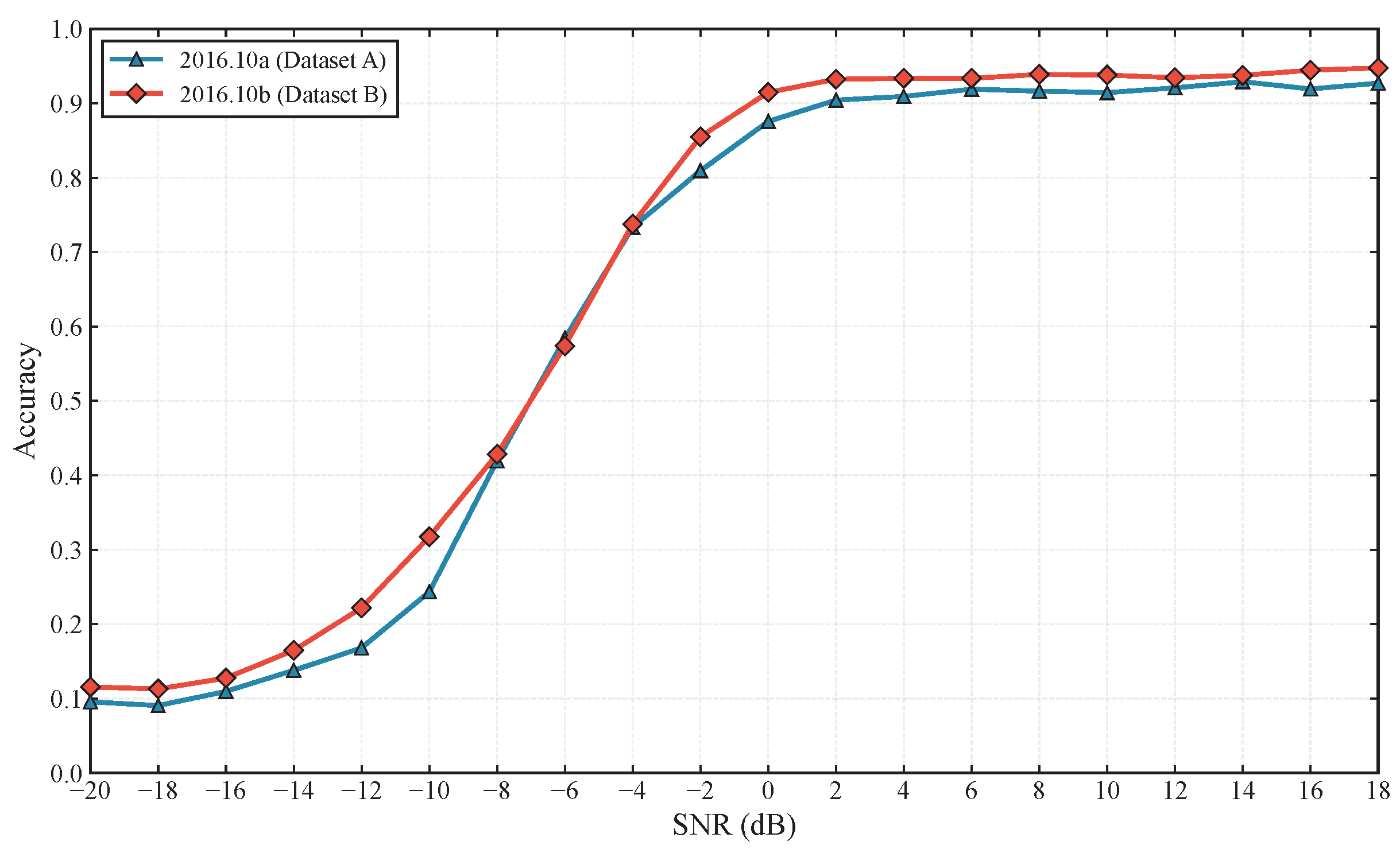
Table 7 reports classification accuracy at each of the 20 SNR levels on RadioML 2016.10A (11 classes, 44,000 test samples) and RadioML 2016.10B (10 classes, 240,000 test samples). Overall accuracy, defined as the unweighted mean over all test samples, reaches 62.76% on 2016.10A and 65.00% on 2016.10B.
Table 7 and Figure 2 show that the largest dataset gap occurs at 12 to 10 dB, where the 2016.10B advantage peaks at about 7 pp before narrowing at higher SNR.
To understand which specific modulation pairs account for the remaining errors, we turn to the per-class accuracy and confusion matrix analysis below.

5.2. Per-Class Accuracy and Confusion Matrix Analysis

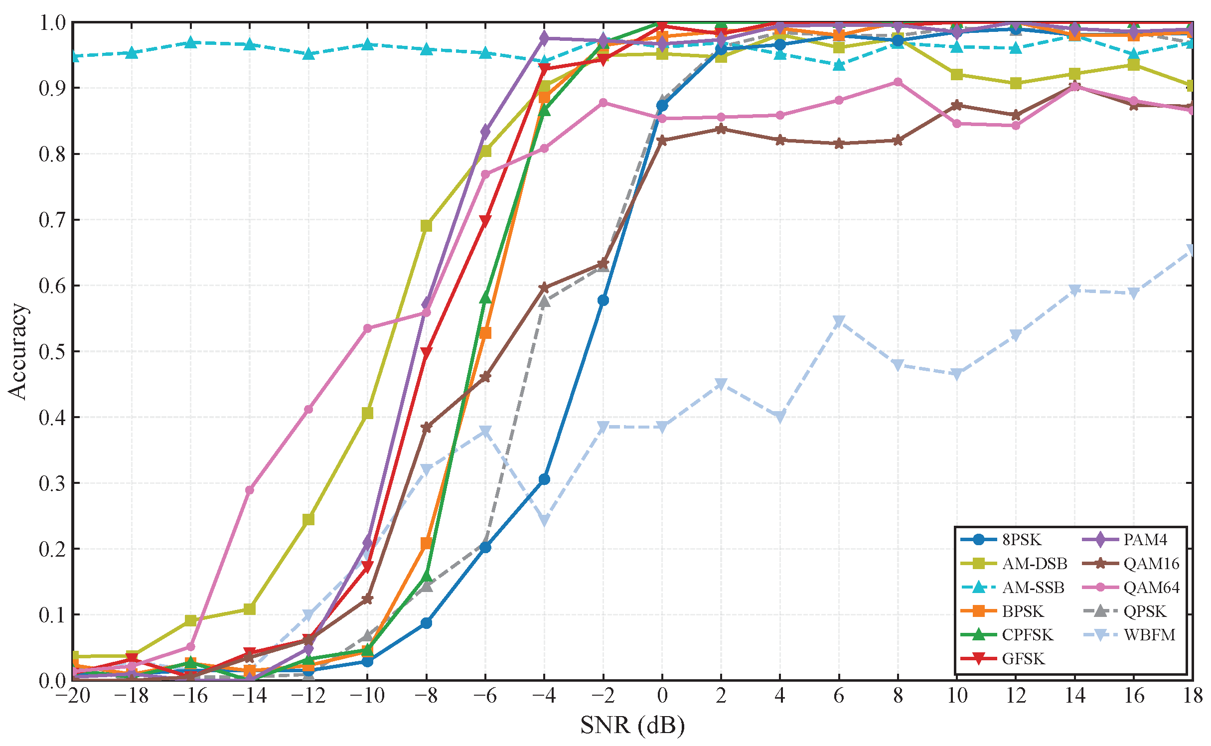
Figure 3 shows per-class accuracy versus SNR for RadioML 2016.10A. On 2016.10A, constant-envelope modulations (BPSK, QPSK, 8PSK, CPFSK, GFSK) converge to near-perfect accuracy above 0 dB, whereas QAM constellations plateau at 85–92% at high SNR due to intra-QAM confusion.
Notably, AM-SSB on 2016.10A achieves an anomalous near-perfect accuracy (approximately 95%) across the entire SNR range. This is not a genuine model capability but rather a dataset artefact—as Shao et al. noted in IQFormer [11], the AM-SSB signals in the RadioML 2016.10A synthetic generation process were inadvertently contaminated by pure noise, so the model essentially classifies noise-like samples as AM-SSB regardless of SNR. To separate this artefact from the remaining 2016.10A evaluation, we additionally exclude samples whose ground-truth label is AM-SSB and compute the macro-averaged recall over the remaining ten classes. The resulting value is 59.45%, compared with the original 62.76% overall accuracy on RadioML 2016.10A. Because prior RadioML 2016.10A studies commonly report the complete 11-class overall accuracy, we retain the full-dataset metric for literature comparison and present the AM-SSB-excluded value as a sensitivity check.
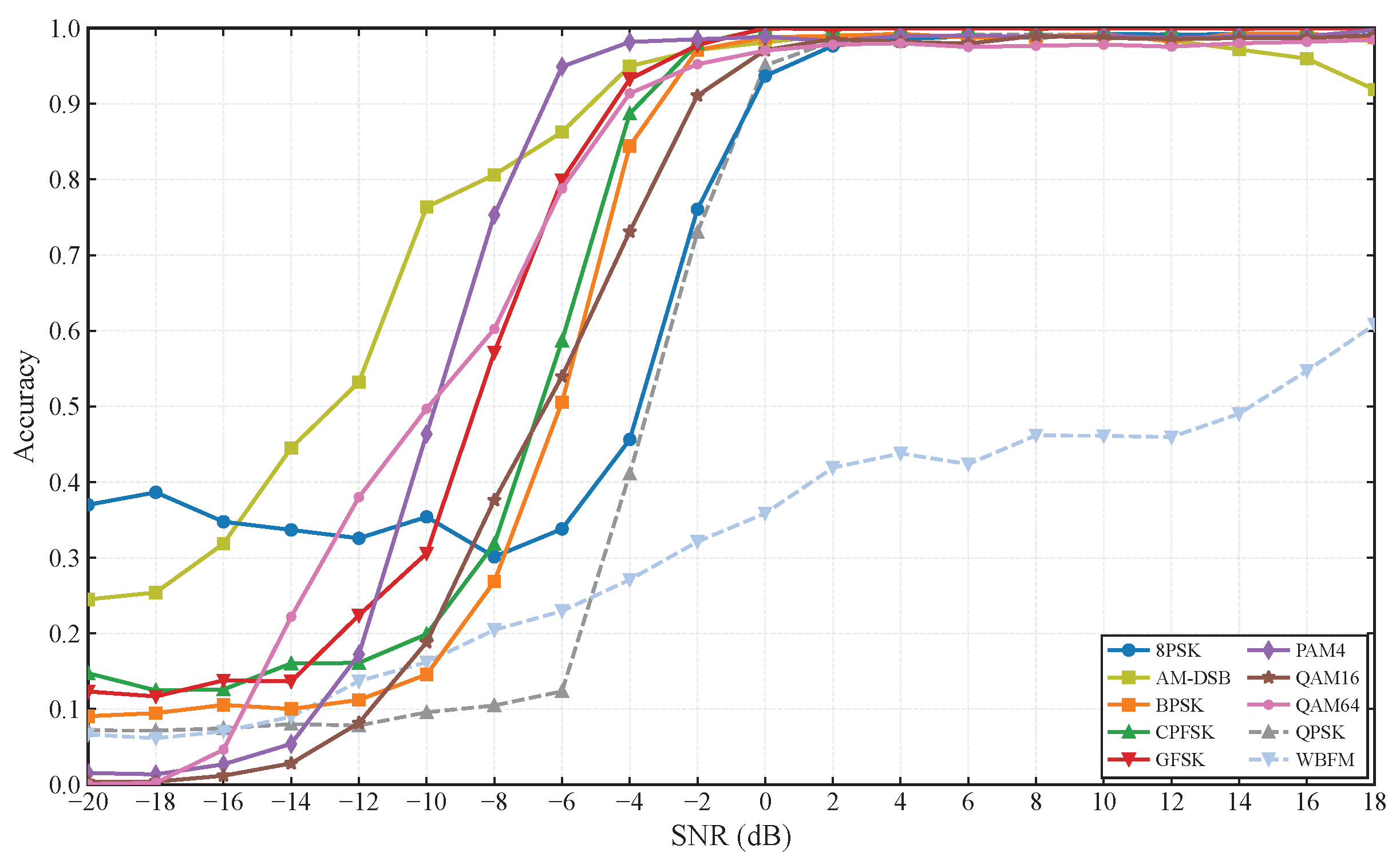
Figure 4 shows the corresponding per-class accuracy curves for RadioML 2016.10B. Every class except WBFM exceeds 90% accuracy at 0 dB. WBFM remains the hardest class, reaching only 48% at + 10 dB—consistent with the confusion-matrix observation that WBFM samples are systematically misrouted to AM-DSB.
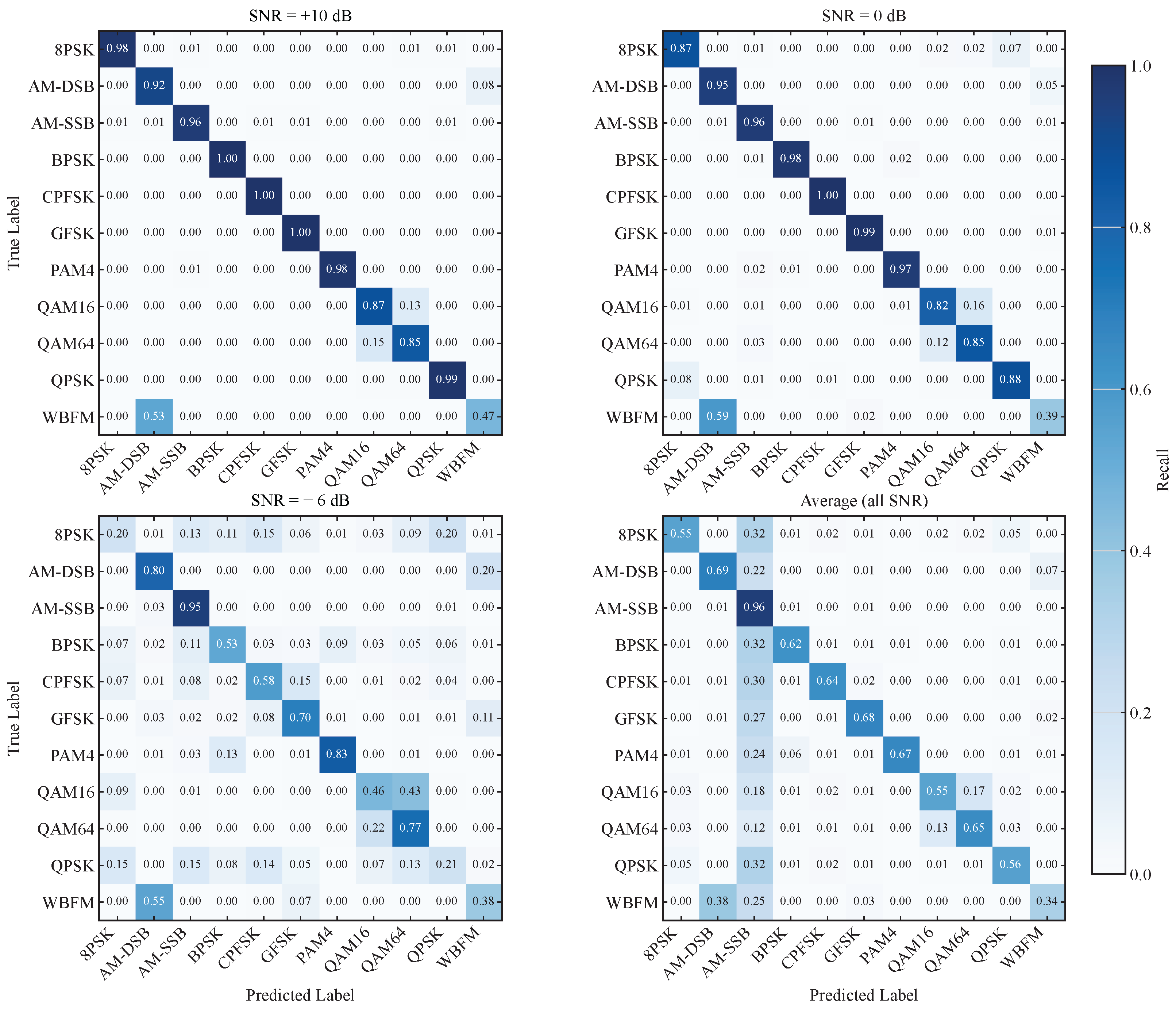
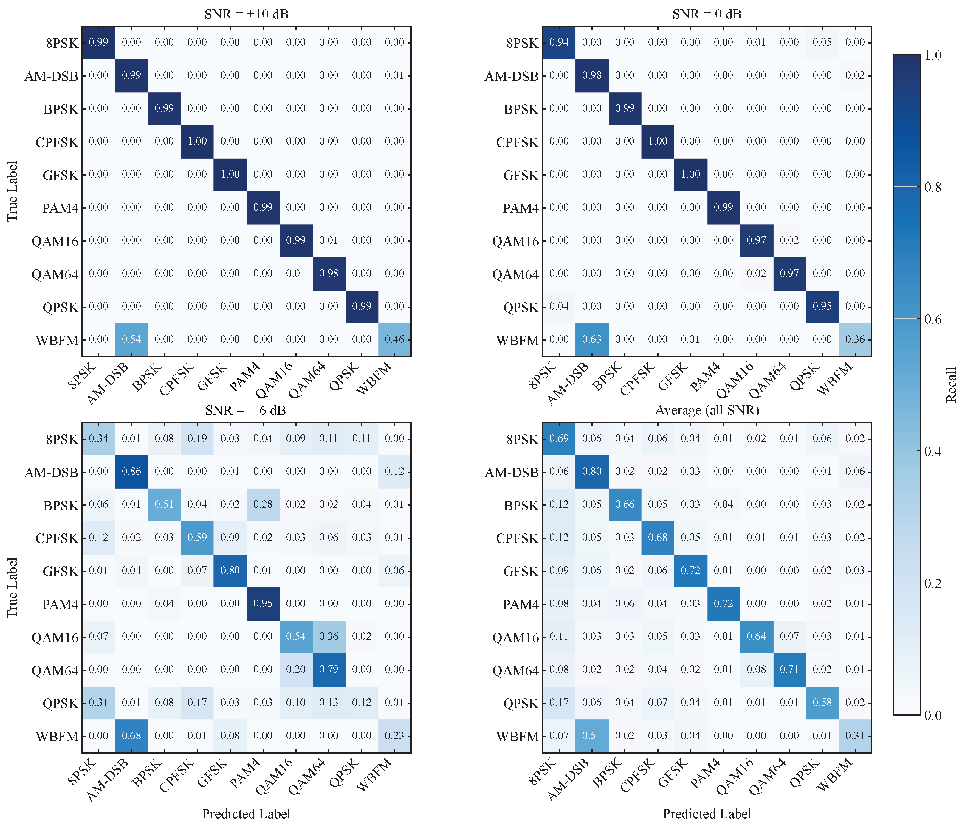
A finer look at the high-SNR confusion matrix in Figure 5 reveals that the matrix shows most classes achieving recall above 0.95, with QAM16↔QAM64 as the notable exception—these two share ring-structured constellations that differ only in density, and the cumulant-based expert features partially but not fully resolve them. At 0 dB, constant-envelope modulations retain a near-diagonal pattern, and off-diagonal mass concentrates within the QAM family (QAM16↔QAM64) and the AM–FM pair (AM-DSB↔WBFM). At 6 dB the behaviour becomes class-dependent: CPFSK and GFSK retain recall above 0.90 thanks to their strong FM signatures, while WBFM recall drops below 0.50 and QAM64 recall falls to roughly 0.50.
The 2016.10B confusion matrices shown in Figure 6 are notably cleaner at moderate and high SNR because AM-SSB is no longer competing with AM-DSB and WBFM. At 0 dB, most classes reach recall above 0.90, with BPSK, CPFSK, GFSK, and PAM4 at or above 0.98. The dominant residual confusion is AM-DSB↔WBFM: AM-DSB exhibits high recall (0.98) but only moderate precision (0.61) because WBFM is frequently mistaken for AM-DSB; WBFM itself suffers from low recall (0.36). These two share spectral-envelope characteristics that make them hard to distinguish even at moderate SNR. At 6 dB, the QAM constellations fragment while CPFSK and GFSK retain strong recall.
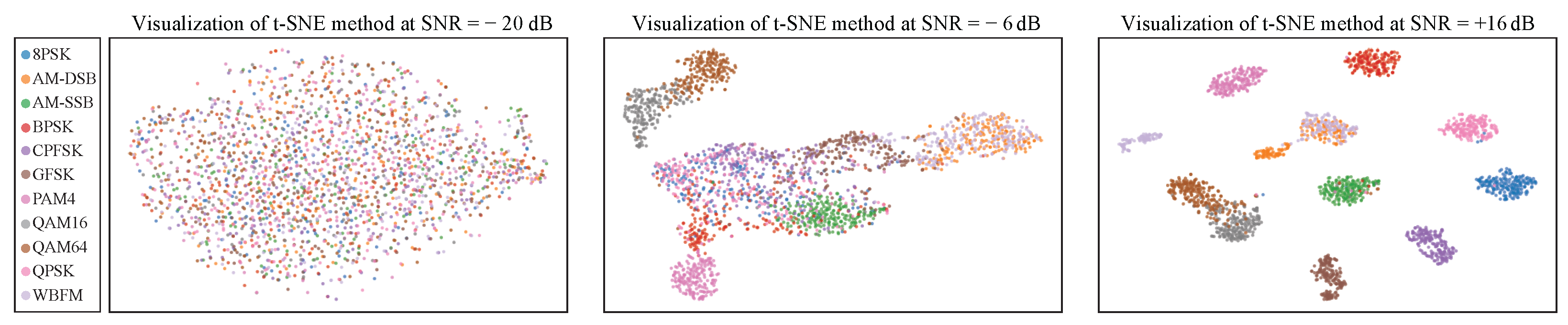
Figure 7 shows t-SNE projections of the fused representation h fusion on RadioML 2016.10A at 20 dB, 6 dB, and + 16 dB. At 20 dB, samples from different modulations are heavily intermixed, consistent with the near-random classification observed in this regime. By 6 dB, FM and PSK families begin to separate, whereas QAM and AM samples still share overlapping regions. At + 16 dB, most modulation types form compact, well-separated clusters. The remaining overlap between AM-DSB and WBFM agrees with the corresponding confusion-matrix pattern.
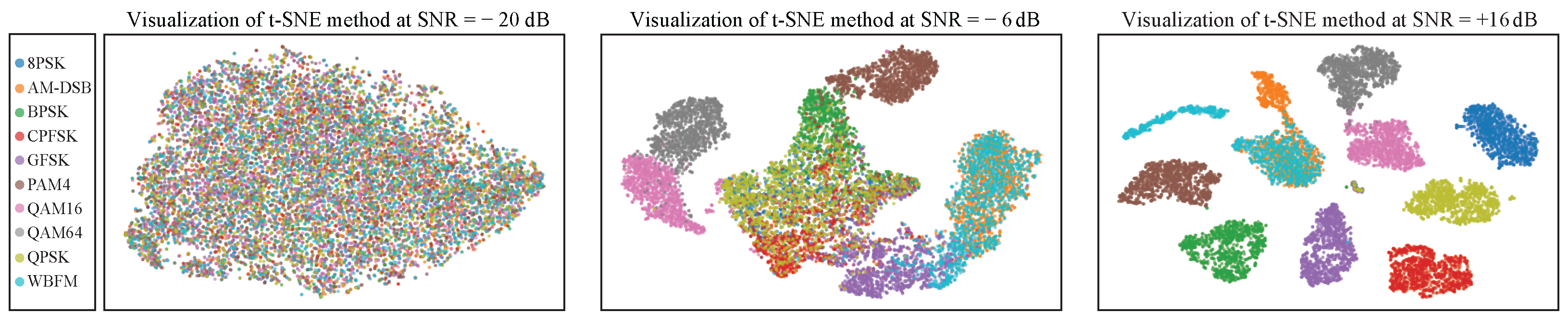
Figure 8 presents the corresponding RadioML 2016.10B projection under the same SNR settings. The overall family-level arrangement is similar to that on 2016.10A, but the clusters are more compact and the margins between neighbouring groups are wider. Without the AM-SSB class, the regions near AM-DSB and WBFM are less crowded, and BPSK and CPFSK appear more clearly separated. AM-DSB also forms a more compact cluster, consistent with the 2.24 pp higher overall accuracy on RadioML 2016.10B reported in Table 7.
Taken together, the per-SNR, per-class, confusion-matrix, and embedding analyses identify three performance bottlenecks. At extremely low SNR, the available modulation-specific information is too weak and the fused representations remain poorly separated. In the transition region around 6 to 0 dB, the temporal and expert branches become simultaneously informative but imperfect, which is where adaptive fusion has the largest effect. At higher SNR, the dominant errors are no longer caused mainly by additive noise but by intrinsic class similarity, especially QAM16/QAM64 and AM-DSB/WBFM. The AM-SSB behaviour on RadioML 2016.10A is treated separately as a dataset artefact rather than as a genuine high-SNR recognition advantage.

5.3. Comparison with Existing Methods

5.3.1. Cross-Paper Comparison with Published AMC Methods

We now situate LGP-Net within the broader landscape of recent AMC methods. Since RadioML 2016.10A/B impose no canonical train/test split, reported accuracies across the literature may diverge by 1–3 pp because of partitioning choices alone; variations in preprocessing pipelines and evaluation protocols can further compound this gap.
All performance values in Table 8 are taken directly from the respective publications, and where identical-protocol replication is unavailable we emphasise the parameter-efficiency axis as a comparison dimension that is invariant to split choice.
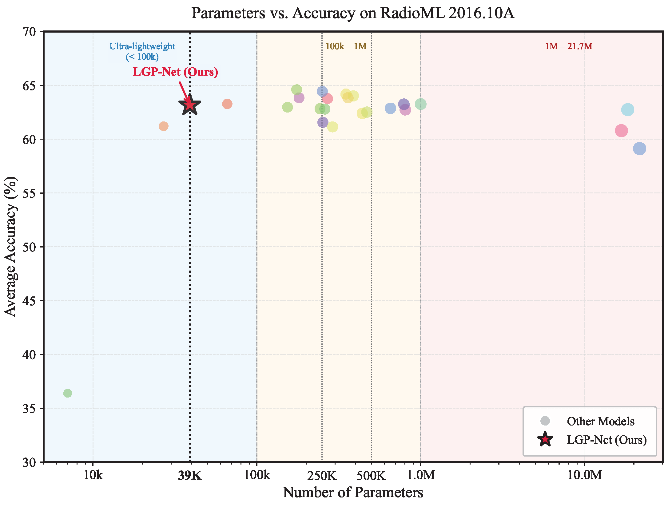
As summarised in Table 8, LGP-Net shows a favourable accuracy–efficiency trade-off compared with recent published works. For instance, TCN–Mamba [19] employs 21.7 M parameters in 2025 yet achieves 59.12% on 2016.10A, whereas MFCA–Transformer [13] reaches 62.74% with 18.35 M parameters, marginally trailing our 62.76% while using three orders of magnitude more parameters.
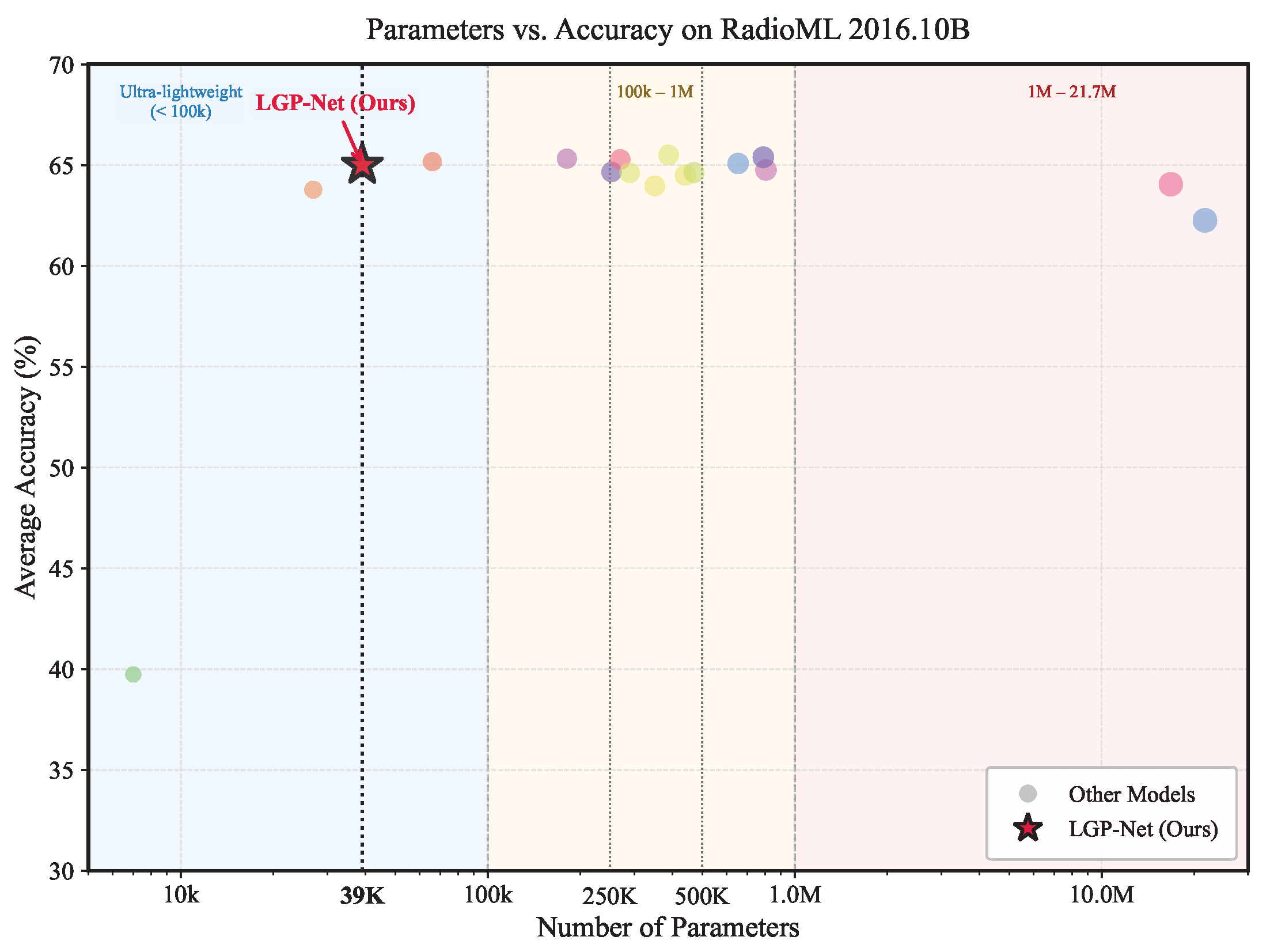
On 2016.10B, our model attains 65.00% using 38,860 parameters, a footprint far smaller than CC–MSNet (654 k, 65.08%) [41], ICRNNA (790 k, 65.39%) [42], RLITNN (181 k, 65.32%) [44], and CBADNN (388 k, 65.50%) [46]. This comparison indicates that LGP-Net achieves competitive accuracy at a substantially lower parameter cost, supporting its intended role in resource-constrained edge-oriented AMC.
Figure 9 visualises the parameter–accuracy trade-off on RadioML 2016.10A against recently published (2024–2026) lightweight AMC methods, with detailed numbers provided in Table 8. LGP-Net (red star) occupies the sub-100 k-parameter zone while reaching accuracy comparable to architectures in the 100 k–1 M range.
Figure 10 presents the corresponding parameter–accuracy scatter for RadioML 2016.10B. As illustrated, LGP-Net (red star) achieves accuracy comparable to many models in the middle and upper-right regions of the plot, while its leftward position on the horizontal axis indicates a much lower parameter overhead.
The cross-paper comparison provides broad literature context, but the absence of a canonical RadioML split still limits strict fairness. We therefore complement it with a same-protocol comparison in which representative lightweight baselines are trained and evaluated under the same local setting as LGP-Net.

5.3.2. Comparison with Reimplemented Same-Protocol Lightweight Baselines

To reduce the uncertainty caused by cross-paper differences in data partitioning, preprocessing, random seeds, and implementation details, we further reimplemented several representative lightweight AMC baselines under the same experimental protocol as LGP-Net. The selected baselines cover recurrent, convolutional, complex-valued, parameter-efficient, and ultra-lightweight designs, including MCLDNN [15], SCNN [18], MCNet [16], PET-CGDNN [17], DAE [6], and ULCNN [14]. Table 9 reports the number of trainable parameters on RadioML 2016.10A and RadioML 2016.10B, the corresponding overall accuracy, the mean accuracy across the two datasets, the mean accuracy at 0 dB, and two deployment-oriented memory indicators.
The results show that LGP-Net provides a favourable balance between recognition accuracy and lightweight deployment cost. Although DAE and ULCNN use fewer parameters, their mean accuracies are lower by 2.20 and 2.30 percentage points, respectively. MCLDNN reaches a slightly higher mean accuracy at 0 dB, but it requires more than 400,000 parameters and an estimated INT8 model size of 0.39 MB. In contrast, LGP-Net achieves the highest mean accuracy in this same-protocol comparison, 63.88%, while requiring only 39,019 parameters on RadioML 2016.10A, 38,860 parameters on RadioML 2016.10B, an estimated INT8 model size of 0.04 MB, and 26 KB peak activation memory. These results support the intended design goal of LGP-Net: it is not the smallest network in isolation, but it offers a compact and accuracy-oriented trade-off for lightweight AMC.

5.4. Hardware Efficiency and Deployment-Oriented Feasibility

The same-protocol comparison above shows that LGP-Net occupies a compact accuracy–efficiency regime relative to reimplemented lightweight baselines. We further analyse whether this compactness translates into practical deployment-oriented evidence. The number of trainable parameters alone is insufficient for this purpose; model storage, peak activation memory, host-side inference latency, quantisation behaviour, and export consistency must also be considered.
Table 10 summarises the hardware-efficiency profile of LGP-Net. The MAC and floating-point operation (FLOP) counts were calculated analytically per layer from the network equations and cross-checked with the parameter breakdown in Table 4. The estimated INT8 parameter storage follows the same one-byte-per-parameter estimate used in the same-protocol lightweight-baseline comparison, whereas the FP32 model size and total inference memory are reported for the floating-point checkpoint.
The peak activation footprint is 26.00 KB, which is below the 256–512 KB on-chip SRAM budget of many Cortex-M4/M7-class microcontrollers. Together with the 0.04 MB estimated INT8 parameter storage, this indicates a compact memory budget for resource-limited inference settings. The latency values in Table 10 provide host-side reference measurements: single-sample classification completes in 4.09 ms on a CPU-only single-thread setting, while CUDA batch = 128 yields 9.3–9.7 μ s amortised latency per sample for high-throughput spectrum-monitoring pipelines.
To further address quantisation and deployment-format concerns, Table 11 reports post-training quantisation (PTQ) and export probes on trained LGP-Net checkpoints. These probes evaluate whether the compact model preserves recognition behaviour after dynamic INT8 PTQ and whether the trained checkpoint can be represented by unrolled deployment-format graphs with identical or near-identical predictions.
These results complement the memory indicators in Table 10. Dynamic INT8 post-training quantisation reduces the serialised state size while causing less than 0.5 percentage-point accuracy degradation. The TFLite export probes further show that the trained checkpoint can be converted into unrolled deployment-format graphs while preserving identical or near-identical predictions. The resulting graphs contain no WHILE control-flow operator or Flex dependency, supporting software-side deployment-format feasibility. We therefore frame these results as deployment-oriented feasibility evidence and leave target-board kernel tuning and power profiling to future hardware-specific benchmarking.

5.5. Ablation Study

After establishing the accuracy, comparison, and deployment-oriented efficiency profile of LGP-Net, we next isolate the contribution of each architectural component by comparing LGP-Net against a set of ablation variants trained under the identical protocol on RadioML 2016.10A. The 2016.10A benchmark is used for the main ablation analysis. To examine whether the same component-level trend persists on RadioML 2016.10B, we further report the corresponding major-component ablation on that dataset.
Three SNR points are highlighted in the following tables: 6 dB represents the transitional regime where the two branches are most competitive, 0 dB marks the beginning of the high-accuracy plateau, and + 10 dB represents the high-SNR regime where the temporal branch is most informative.
The study is organised into four parts: major-component ablation, expert-group ablation, temporal-branch sub-module ablation, and fusion-rule comparison with class-level gate evidence. The fine-grained expert-feature and temporal sub-module ablations are used as diagnostic analyses of the internal design on RadioML 2016.10A, while cross-dataset support for the main architectural components and the gate mechanism is provided on RadioML 2016.10B.

5.5.1. Major Component Ablation

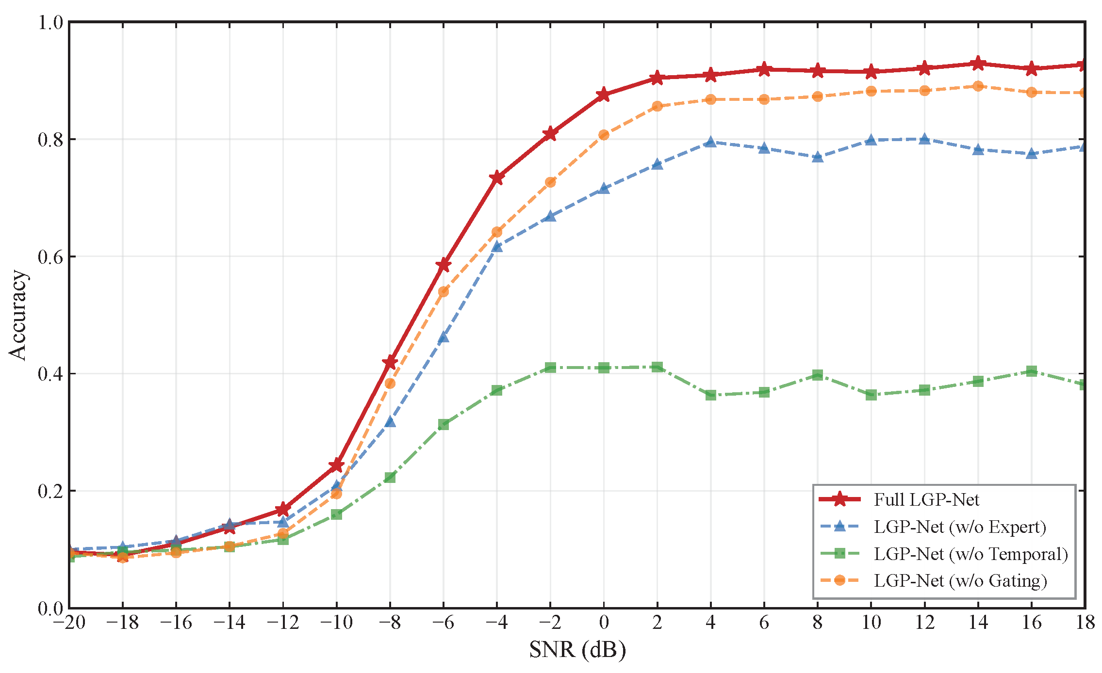
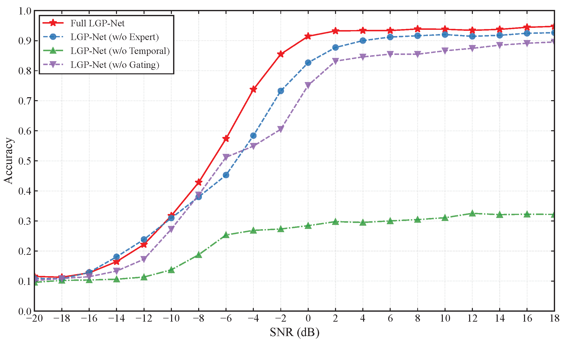
Figure 11 and Table 12 summarise the major-component ablation results, while Figure 12 shows the corresponding per-SNR curves on RadioML 2016.10B.
Removing the temporal branch forces the network to rely on the expert branch alone. Overall accuracy collapses from 62.76% to 29.25%, a loss of 33.5 pp. The damage is unevenly distributed across SNR: at 0 dB the expert-only variant reaches 40.99%, well above the 9.09% random-guess floor but still 46.6 pp below the full model.
The expert branch delivers a modest yet consistent performance boost. Dropping this component reduces overall accuracy by 9.41 pp, with the largest performance gap of 15.99 pp appearing at 0 dB. The difference can be seen as early as 6 dB: the full model obtains 58.50%, whereas the version without the expert branch reaches 46.25%. At low SNR, the expert features retain discriminative power that the temporal branch has already lost to noise. These features are calculated directly from raw IQ data, prior to any normalisation.
A fixed 50/50 average of the two branches incurs an overall accuracy penalty of 4.24 pp relative to the learned gate. The largest gap appears around 0 dB, where the averaged fusion strategy attains 80.71% compared with 87.57% for the full model with adaptive gating. This finding highlights the importance of learning branch weights rather than using a uniform weighting scheme.
The magnitude of each penalty differs between the two datasets, but the component ranking and the positive contribution of each major component are consistent. On RadioML 2016.10B, removing the temporal branch remains by far the most destructive ablation, dropping overall accuracy from 65.00% to 23.62%. The expert branch still provides a positive contribution away from the high-SNR ceiling, and the learned gate remains beneficial, with the fixed-fusion variant incurring a 7.50 pp overall penalty and a 16.34 pp gap at 0 dB. The corresponding per-SNR curves are shown in Figure 12.

5.5.2. Expert Feature Group Ablation

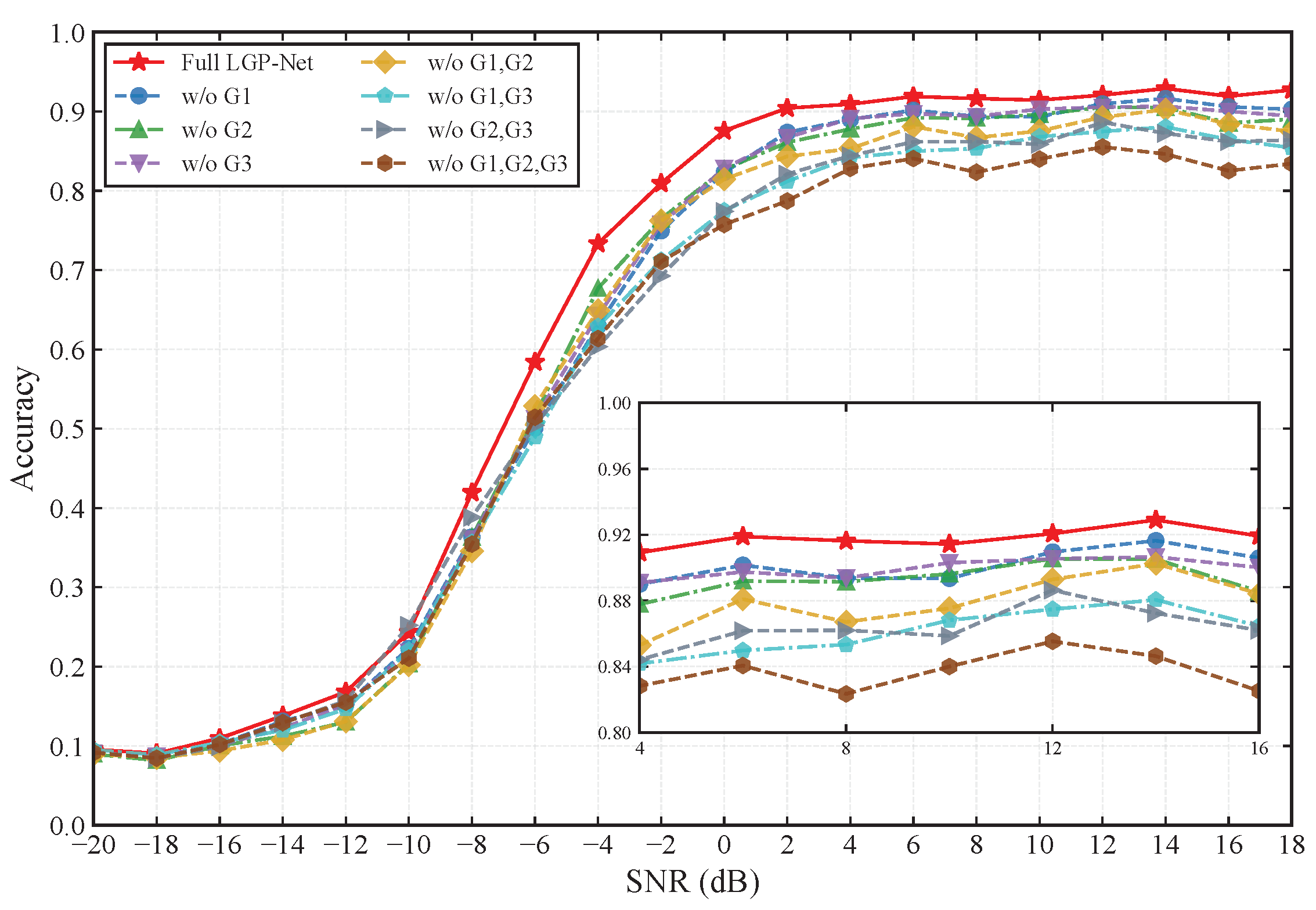
The 11 expert features presented in Table 3 are divided into three groups (G1–G3). We evaluate all possible group subsets, zeroing the removed features before the expert MLP while keeping all other elements unchanged.
Figure 13 presents per-SNR accuracy of the eight variants. All curves intersect at the random-guessing floor below 10 dB. Above 0 dB they diverge, with the full model yielding the highest accuracy.
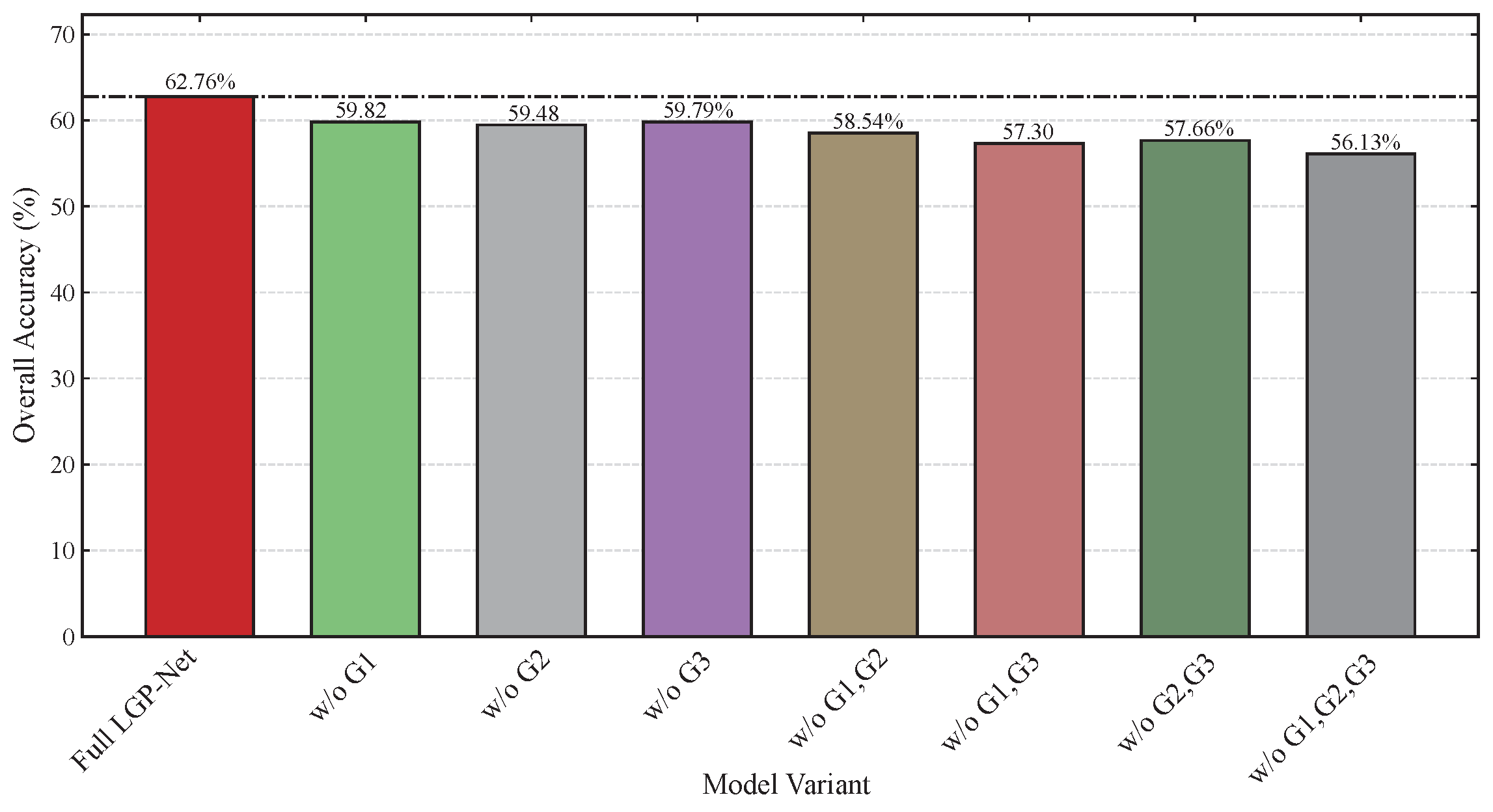
Figure 14 summarises the overall accuracy. Pairwise removals yield 57–59%, and removing all three groups gives 56.13%, a 6.63 pp deficit. The penalties are non-additive: G1 can be removed at a cost of 2.94 pp, but when both G1 and G2 are removed together, the cost becomes 4.22 pp rather than the sum of the individual costs. This pattern indicates partial redundancy among the groups, with some statistics being encoded through more than one feature group.

5.5.3. Sub-Module Ablation of the Temporal Branch

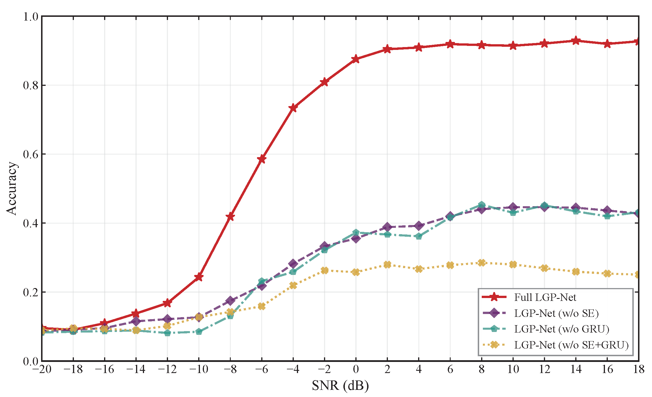
Figure 15 and Table 13 evaluate three variants: SE attention removed, GRU replaced by temporal average pooling, and both removed.
Removing SE reduces overall accuracy by 33.49 pp. Without per-channel recalibration, noise-corrupted channels propagate degradation into deeper layers. At 6 dB, accuracy drops from 58.50% to 21.84%. Replacing GRU with average pooling incurs a comparable 34.76 pp penalty, because average pooling discards the event ordering that distinguishes, for instance, FM frequency sweeps from PM phase transitions.
Joint removal of SE and GRU yields 20.31% overall—approximately 9 pp below the expert-only variant (29.25%) from Table 12. Removing the entire temporal pathway is therefore preferable to retaining an unfiltered one because raw DSConv outputs without SE or GRU introduce noise-driven features that the downstream gate cannot fully discount. SE and GRU are therefore not merely incremental additions; they are needed to make the convolutional stack a functional feature extractor.

5.5.4. Fusion Rule Comparison

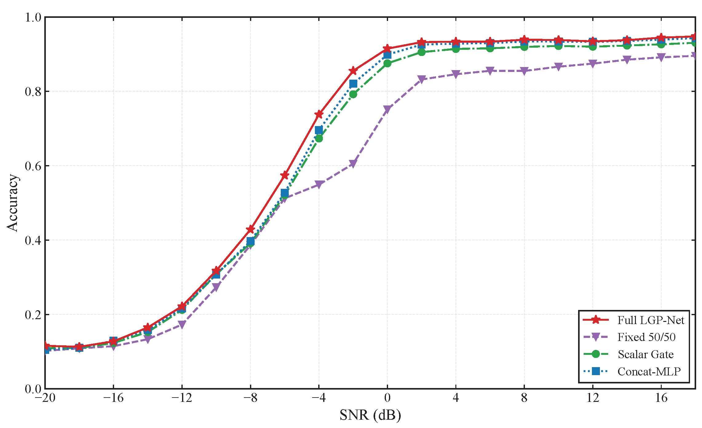
To examine whether the gain comes merely from using a learnable combiner or from the proposed per-dimension gate, we compare Full LGP-Net with three representative fusion rules on RadioML 2016.10B: fixed 50/50 averaging, a sample-wise scalar gate, and a feature-level Concat-MLP. Table 14 summarises the overall accuracy, selected SNR points, and the transition-region average.
Here, Transition denotes the mean accuracy over 6 , 4 , 2 , and 0 dB, and Gain over Fixed is measured as the overall-accuracy improvement over the fixed 50/50 baseline. Fixed averaging is clearly insufficient, reaching only 57.50% overall accuracy and 60.45% in the transition region. Concat-MLP and the sample-wise scalar gate recover much of this loss, improving the overall accuracy to 63.79% and 62.68%, respectively. Nevertheless, Full LGP-Net remains the highest-performing variant in this comparison, with 65.00% overall accuracy and 77.04% transition accuracy. Its transition-region advantage is 3.48% over Concat-MLP and 5.49% over scalar gate, indicating that the per-dimension gate is most useful when the two branches carry complementary but imperfect evidence.
Figure 16 visualises the corresponding per-SNR trends for the fusion rules on RadioML 2016.10B.
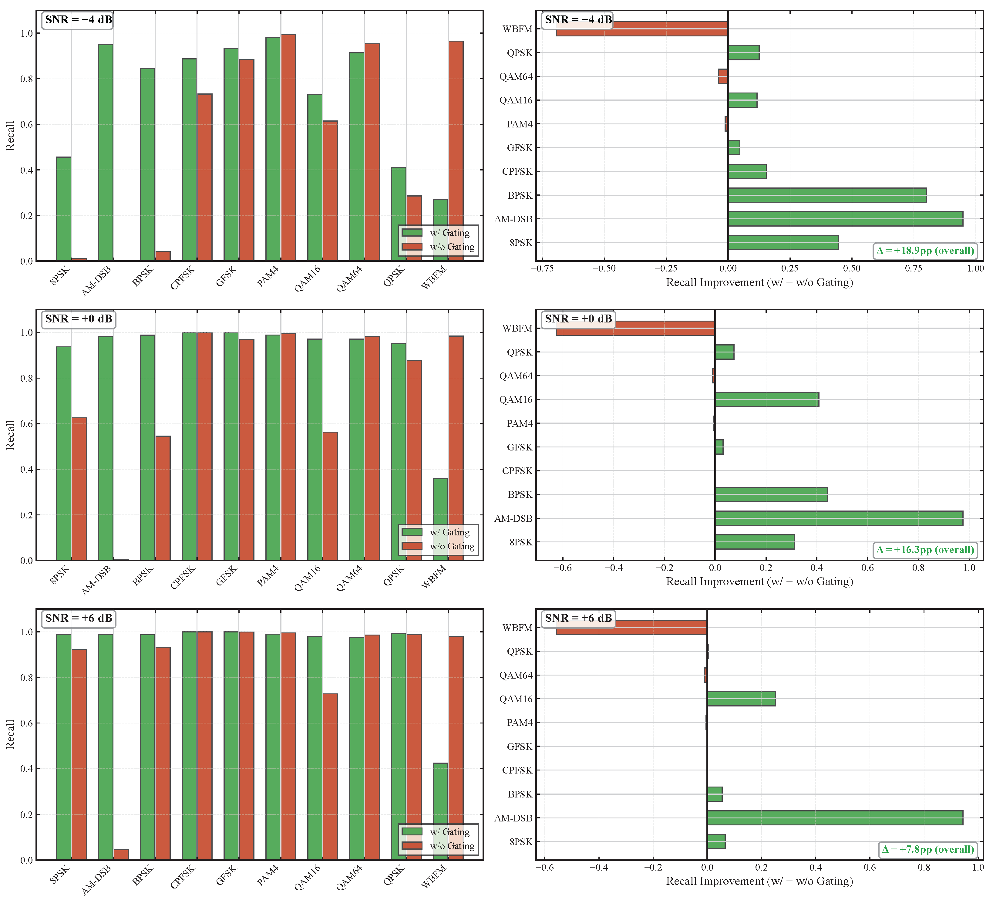
The aggregate comparison is further supported by class-level recall between the full model and a fixed 50/50 fusion variant at three SNR levels ( 4 , 0, + 6 dB), as visualised in Figure 17. The overall recall gain from the learned gate is + 18.9 pp at 4 dB, + 16.3 pp at 0 dB, and + 7.8 pp at + 6 dB.
At 4 dB the two branches are simultaneously unreliable, each producing meaningful but imperfect confidence estimates. The learned gate, which assigns a per-dimension weight to each branch, can therefore better exploit complementary evidence from both, yielding the largest gain over the fixed-weight baseline. At + 6 dB the temporal branch already dominates, so fixed averaging approaches gated performance because there is little residual ambiguity to exploit. The gate achieves this without receiving any SNR label during training.

5.6. Robustness Under Controlled Co-Channel Interference

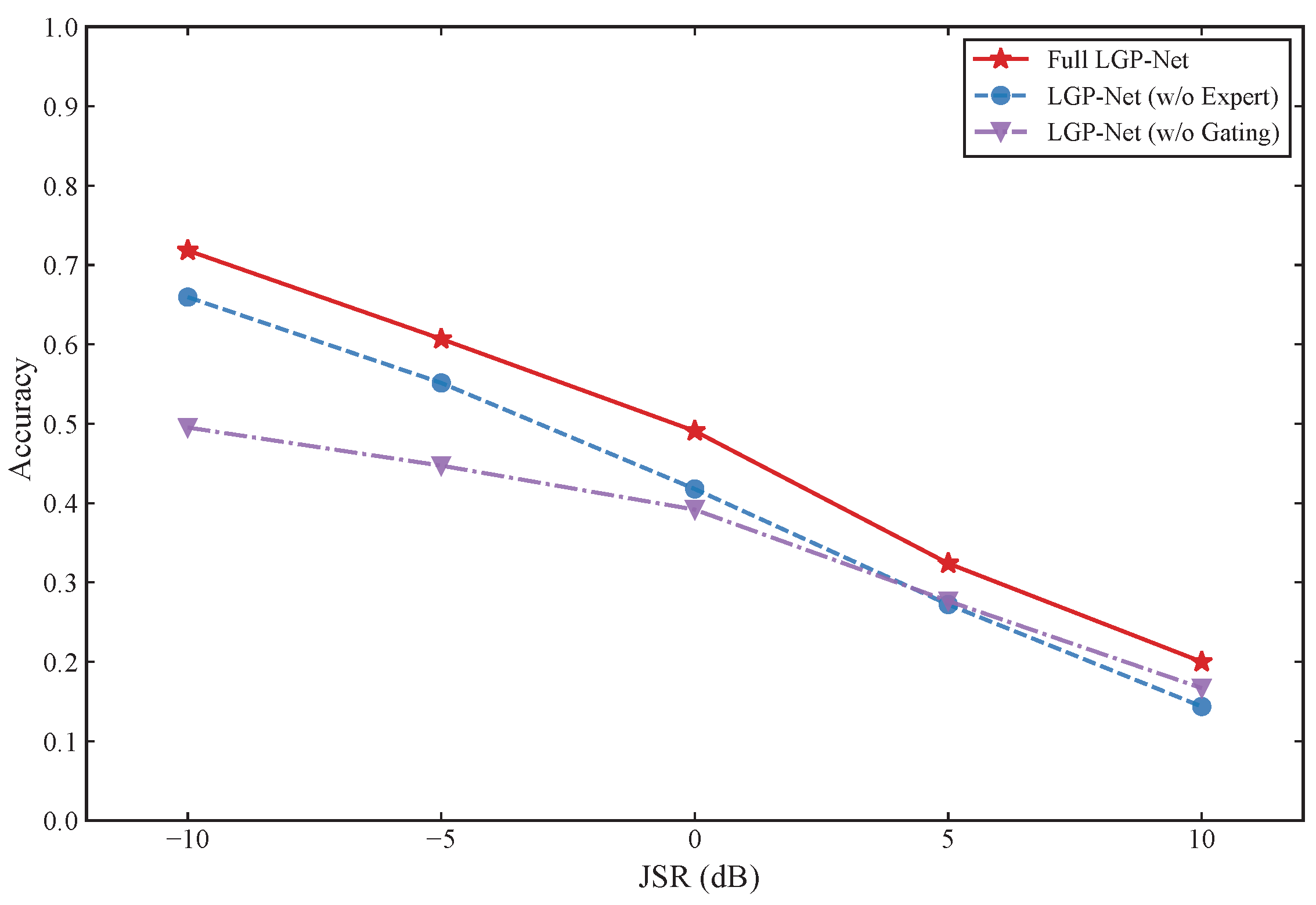
To further probe robustness beyond AWGN-only SNR degradation, we conduct a controlled co-channel interference stress test on RadioML 2016.10B, which is intended to assess representative signal corruption rather than claim complete immunity to all forms of real-world jamming. For each target sample at 0 dB SNR, an interfering sample from a different modulation class is superimposed with a jammer-to-signal ratio (JSR) ranging from 10 to + 10 dB.
The comparison focuses on the w/o Expert and w/o Gating variants because they isolate the two mechanisms most directly related to signal corruption: the physics-informed statistics and the adaptive branch weighting. The w/o Temporal variant is not repeated here because the temporal pathway has already been examined in the component and sub-module ablations; adding it to this interference-specific test would mainly provide another lower-bound diagnostic rather than clarify the jamming-related role of the expert branch and gate.
As shown in Figure 18 and Table 15, the full LGP-Net maintains the highest accuracy across the entire JSR sweep. The advantage is most visible under mild-to-moderate interference: at JSR = 10 dB, adaptive fusion improves accuracy by 22.31 pp over fixed fusion, and at JSR = 0 dB the full model remains 7.30 pp and 9.90 pp ahead of the w/o Expert and w/o Gating variants, respectively.
When JSR increases to +5 and +10 dB, the margins become smaller because the jammer starts to dominate both waveform and statistical evidence. Even at JSR = +10 dB, however, the full model still keeps a 5.63 pp advantage over the w/o Expert variant. This trend supports the role of the expert branch and gate under controlled co-channel corruption, while also showing the expected performance boundary under severe interference.

5.7. Gate Behaviour Analysis

The preceding robustness test evaluates the model under an external signal-corruption scenario. We now examine the internal routing behaviour of the gate to determine whether the learned fusion weights vary coherently with signal quality, gate uncertainty, and modulation class.

5.7.1. Dimension-Level Gate Response

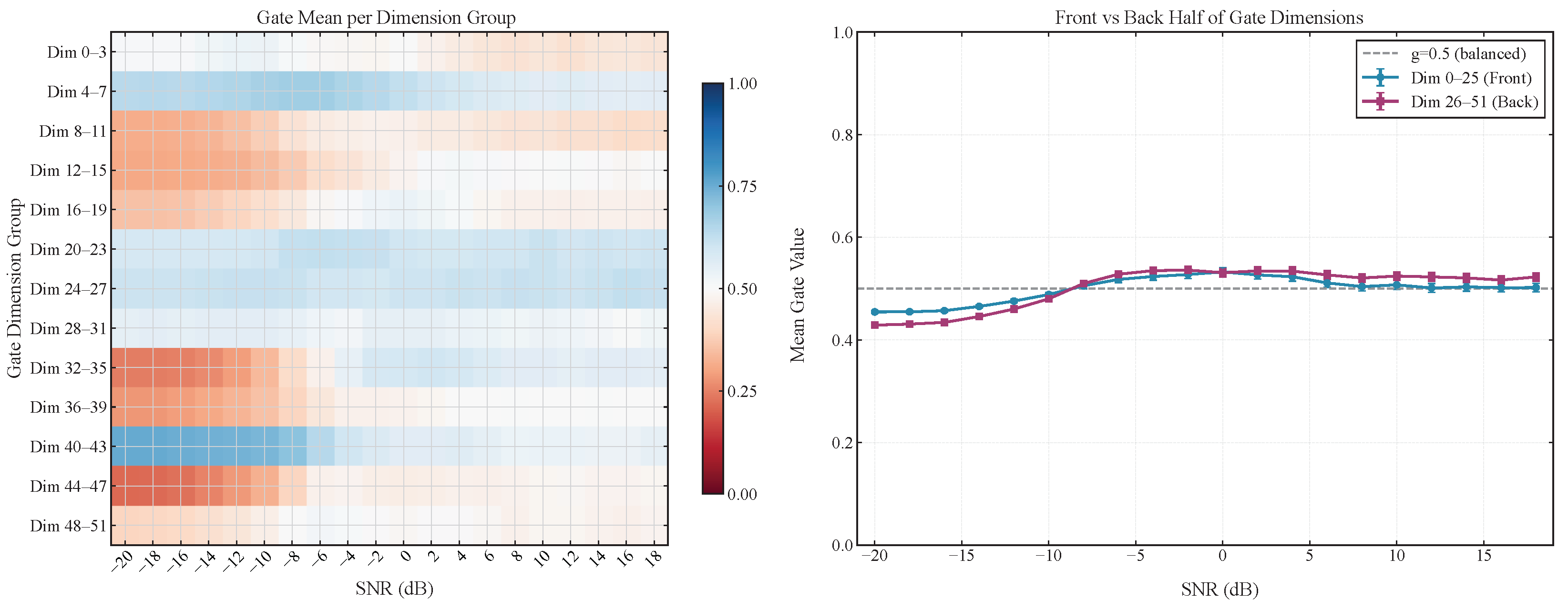
Two views of the 52-dimensional gate vector are shown in Figure 19: a heatmap (left) binning the 52 channels into 13 groups of four and tracking mean activation against SNR, and a front/back half-dimension comparison (right).
The heatmap shows non-uniform responses across dimension groups: some shift toward the temporal branch as SNR increases, others retain expert-branch preference at high SNR, and a few exhibit weak SNR sensitivity. The gate therefore operates as a per-dimension routing mechanism rather than a single scalar knob that globally scales the branch weights of all dimensions combined.
In the right panel, neither half-dimension curve approaches 1 at high SNR. This is partly due to averaging over 52 dimensions, which masks heterogeneity within the vector. More fundamentally, full saturation is not beneficial: modulation pairs such as QAM16/QAM64 and AM-DSB/WBFM continue to benefit from the expert branch’s cumulant features at all SNR levels.

5.7.2. Quantitative Gate Entropy Analysis

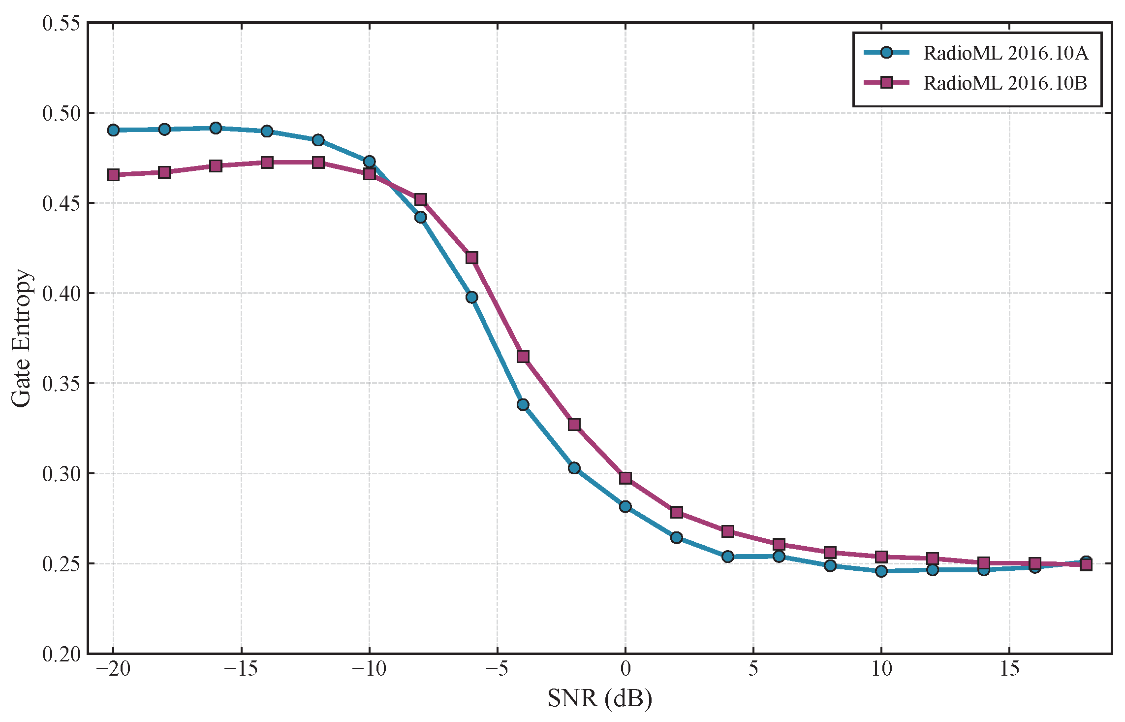
To complement the dimension-level heatmap, we report two quantitative summaries of the learned gate dynamics: the Pearson correlation between the mean gate value and SNR, and the Bernoulli entropy of the per-dimension gate coefficients. The former captures the average shift in routing weight with signal quality, while the latter measures the uncertainty of the branch mixture. Entropy is averaged over all 52 gate dimensions and test samples at each SNR, then grouped into low SNR ( SNR 6 dB), mid SNR ( 4 SNR + 4 dB), and high SNR ( SNR + 6 dB) regimes.
Figure 20 and Table 16 show that the entropy decreases as signal quality improves on both benchmarks. The main drop appears before the high-SNR plateau: on RadioML 2016.10B, the average entropy decreases from 0.461 in the low-SNR regime to 0.307 in the mid-SNR regime; on RadioML 2016.10A, it decreases from 0.470 to 0.288. In the high-SNR regime, the curves level off near 0.25 instead of collapsing to zero, which agrees with the heatmap observation that the fusion does not saturate to a single branch.
The mean gate value is also correlated with SNR, with Pearson coefficients of 0.893 on RadioML 2016.10B and 0.710 on RadioML 2016.10A. The stronger correlation on 2016.10B is consistent with the removal of the anomalous AM-SSB class, whereas the entropy reduction remains visible on both datasets. These statistics support the view that the learned routing responds to signal quality while retaining contributions from both branches, rather than functioning as an explicit SNR estimator.

5.7.3. Gate Value Distribution Across Modulation Classes

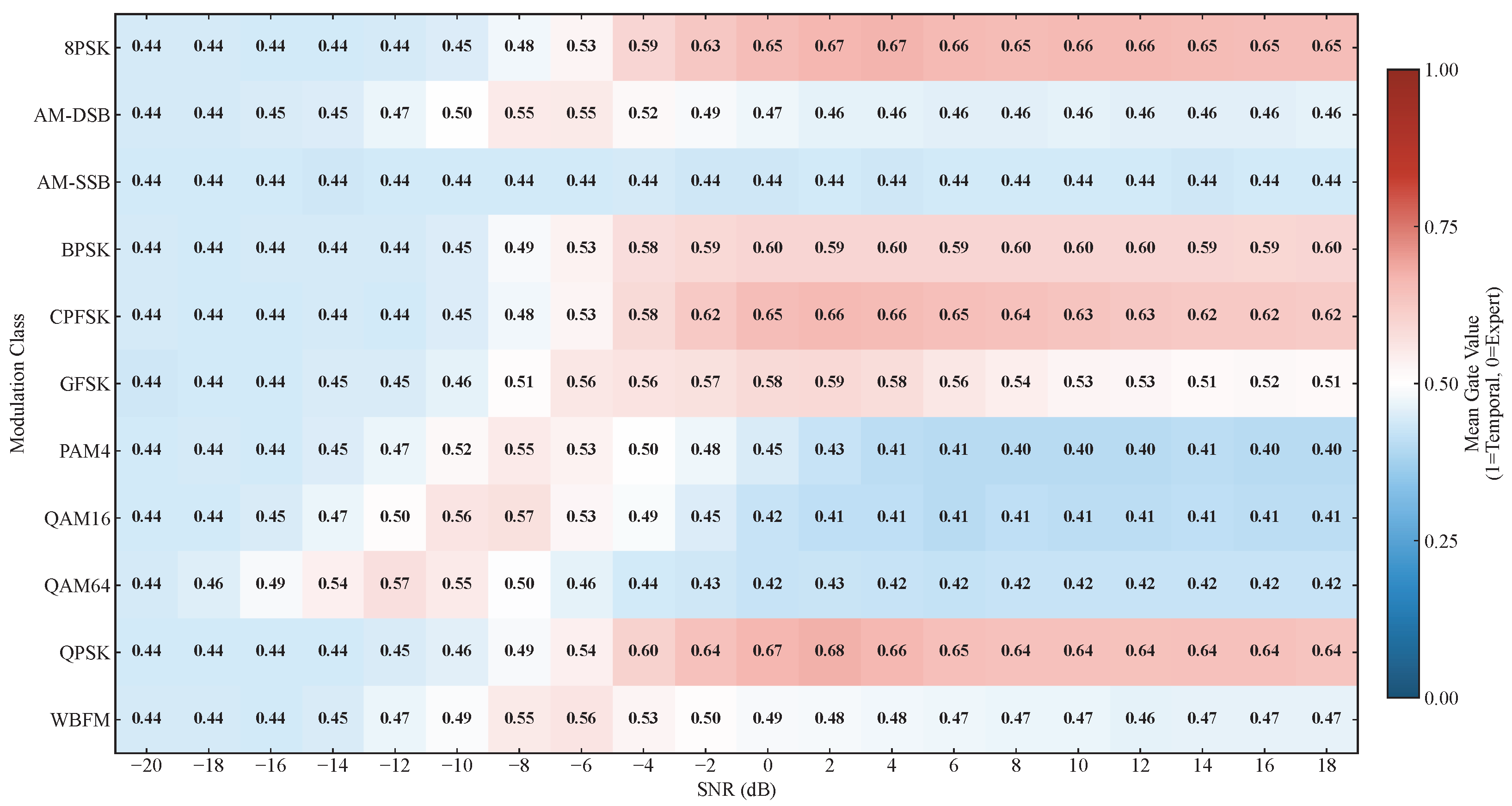
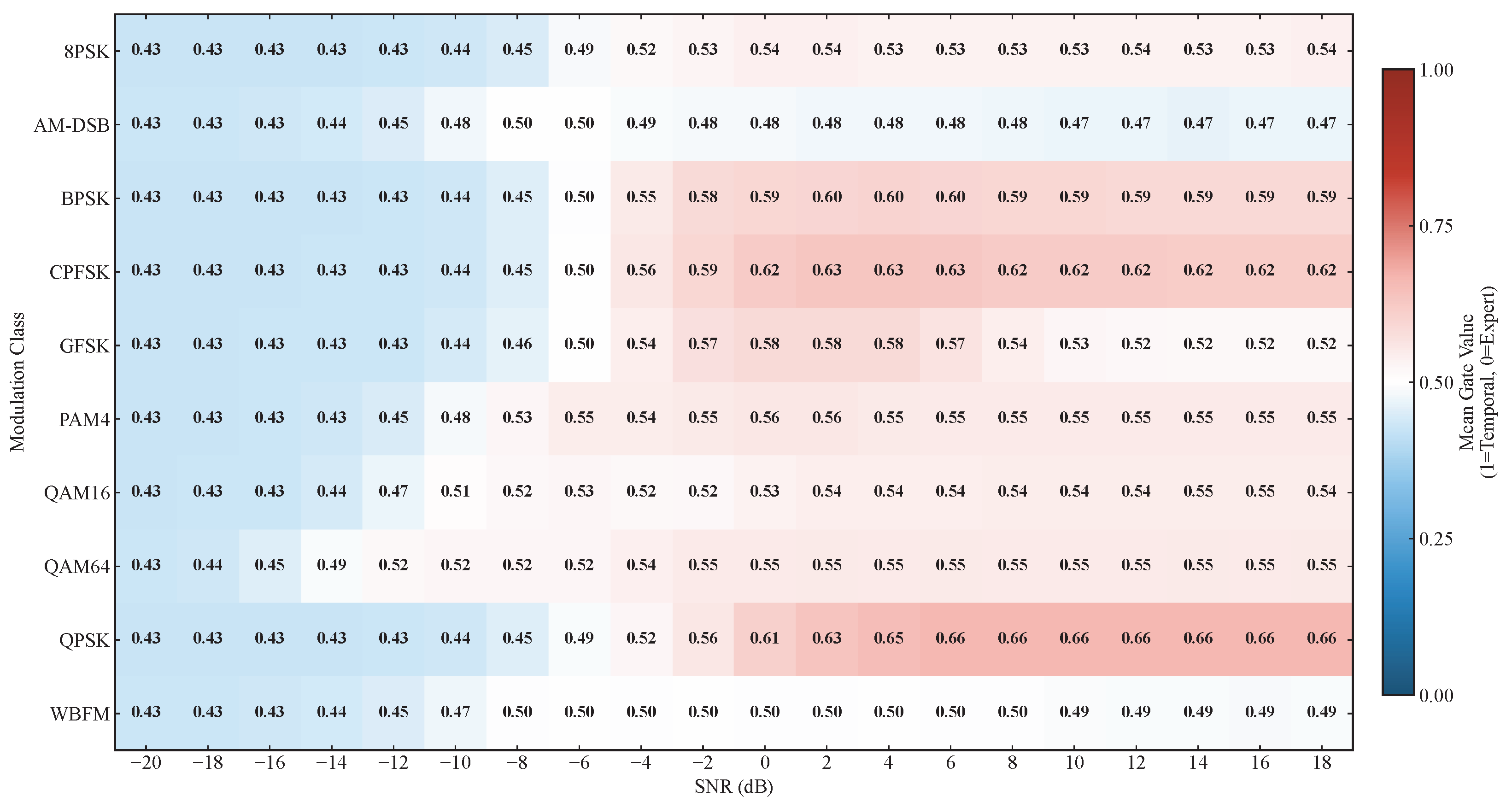
Figure 21 decomposes the mean gate value by modulation class against SNR on RadioML 2016.10A. The colour scale runs from deep blue ( g ¯ < 0.5 , expert-branch preference) through white ( g ¯ 0.5 , balanced) to deep red ( g ¯ > 0.5 , temporal-branch preference).
Gate values at very low SNR ( 20 to 16 dB) tend to be around 0.44 in all classes, suggesting that the gate relies more on the expert branch when temporal features are heavily corrupted by noise. As SNR increases, class-dependent behaviour appears. For modulations with distinct phase or frequency structure, gate values grow monotonically and stabilise above 0.64, indicating that the temporal branch can resolve these waveforms under good channel conditions.
Dense-constellation modulations (QAM64, QAM16, and PAM4), by contrast, exhibit an inverted-V pattern: the gate value rises toward mid-SNR before declining back to 0.41–0.43 at high SNR. This behaviour may reflect the small Euclidean distances between constellation points, which restrict the discriminative power of the temporal branch and encourage the gate to shift weight toward higher-order cumulant characteristics from the expert branch. AM-SSB is a distinct example: its gate value remains near 0.44 across the SNR range, consistent with the known signal-generation defect in this dataset [11].
On RadioML 2016.10B, Figure 22 shows that the removal of the problematic AM-SSB class allows the gate to assign more temporal-branch weight overall, and most classes follow a monotonically increasing trend without the inverted-V pattern seen on 2016.10A. The QAM family and PAM4, which were expert-branch-dominant at high SNR on 2016.10A, have gate values of about 0.55 and 0.54, respectively. This pattern suggests that the temporal encoder can extract useful residual features for constellation discrimination once the label space becomes cleaner.
The two main exceptions are AM-DSB and WBFM, which remain close to the balance line of 0.47–0.50 at high SNR. Because these classes share similar spectral-envelope characteristics, neither branch alone fully resolves the ambiguity, and the gate therefore remains nearly balanced. This behaviour further supports retaining the expert branch for classes where waveform-level representations alone are insufficient.

6. Conclusions

In this paper, we propose LGP-Net, a compact and parameter-efficient automatic modulation classification (AMC) framework designed to address the accuracy–efficiency trade-off in edge-oriented AMC. By coupling a compact temporal encoder with a physics-informed expert branch, the model jointly exploits data-driven waveform representations and noise-aware statistical priors. A key component of LGP-Net is its adaptive, per-dimension gated fusion mechanism. Trained without any explicit signal-to-noise ratio (SNR) labels, the gate learns to adjust the branch balance under severe channel degradation.
The experimental results show that LGP-Net achieves 65.00% overall accuracy on RadioML 2016.10B with 38,860 parameters, remaining competitive with substantially larger architectures. On RadioML 2016.10A, LGP-Net also achieves 62.76% accuracy. In addition, LGP-Net has a 26.00 KB peak activation footprint, host-side single-sample CPU latency of 4.09 ms, dynamic INT8 accuracy retention, and unrolled TFLite export consistency. These measurements and probes indicate its potential for resource-limited, SRAM-constrained deployment scenarios within a compact parameter-and-activation memory budget, and motivate subsequent target-board benchmarking.
In future work, we aim to extend the generalisation capability of LGP-Net by evaluating it on more expansive label spaces, such as the 24-class RadioML 2018.01A benchmark. Furthermore, incorporating advanced cyclostationary or spectral-density descriptors into the expert branch is expected to mitigate residual inter-class confusions, particularly between AM-DSB and WBFM. Finally, target-board benchmarking on FPGA and specialised embedded platforms will be conducted to evaluate board-level latency, energy, and power behaviour in real-world electromagnetic environments.

Author Contributions

Conceptualisation, Z.C. and X.L.; methodology, X.L.; software, X.L.; validation, X.L.; formal analysis, X.L.; investigation, X.L.; resources, Z.C.; data curation, X.L.; writing—original draft preparation, X.L.; writing—review and editing, Z.C. and X.L.; visualisation, X.L.; supervision, Z.C.; project administration, Z.C. All authors have read and agreed to the published version of the manuscript.

Funding

This research received no external funding.

Data Availability Statement

The RadioML 2016.10A and RadioML 2016.10B datasets used in this study were provided by DeepSig Inc. (Arlington, VA, USA) and are licensed under the Creative Commons Attribution–NonCommercial–ShareAlike 4.0 International (CC BY-NC-SA 4.0) License; available at https://www.deepsig.ai/datasets/ (accessed on 25 December 2025). RadioML 2016.10A contains 11 modulation classes (220,000 samples) and RadioML 2016.10B contains 10 classes (1,200,000 samples).

Conflicts of Interest

The authors declare no conflicts of interest.

References

  1. Peng, S.; Sun, S.; Yao, Y.-D. A Survey of Modulation Classification Using Deep Learning: Signal Representation and Data Preprocessing. IEEE Trans. Neural Netw. Learn. Syst. 2022, 33, 7020–7038. [Google Scholar] [CrossRef] [Scilit]
  2. Zhang, F.; Luo, C.; Xu, J.; Luo, Y.; Zheng, F.-C. Deep Learning Based Automatic Modulation Recognition: Models, Datasets, and Challenges. Digit. Signal Process. 2022, 129, 103650. [Google Scholar] [CrossRef] [Scilit]
  3. Swami, A.; Sadler, B.M. Hierarchical Digital Modulation Classification Using Cumulants. IEEE Trans. Commun. 2000, 48, 416–429. [Google Scholar] [CrossRef] [Scilit]
  4. O’Shea, T.J.; Roy, T.; Clancy, T.C. Over-the-Air Deep Learning Based Radio Signal Classification. IEEE J. Sel. Top. Signal Process. 2018, 12, 168–179. [Google Scholar] [CrossRef] [Scilit]
  5. West, N.E.; O’Shea, T. Deep Architectures for Modulation Recognition. In 2017 IEEE International Symposium on Dynamic Spectrum Access Networks (DySPAN); IEEE: New York, NY, USA, 2017; pp. 1–6. [Google Scholar] [CrossRef] [Scilit]
  6. Ke, Z.; Vikalo, H. Real-Time Radio Technology and Modulation Classification via an LSTM Auto-Encoder. IEEE Trans. Wirel. Commun. 2022, 21, 370–382. [Google Scholar] [CrossRef] [Scilit]
  7. Lin, S.; Zeng, Y.; Gong, Y. Modulation Recognition Using Signal Enhancement and Multistage Attention Mechanism. IEEE Trans. Wirel. Commun. 2022, 21, 9921–9935. [Google Scholar] [CrossRef] [Scilit]
  8. Liu, F.; Zhang, Z.; Zhou, R. Automatic Modulation Recognition Based on CNN and GRU. Tsinghua Sci. Technol. 2022, 27, 422–431. [Google Scholar] [CrossRef] [Scilit]
  9. Cai, J.; Gan, F.; Cao, X.; Liu, W. Signal Modulation Classification Based on the Transformer Network. IEEE Trans. Cogn. Commun. Netw. 2022, 8, 1348–1357. [Google Scholar] [CrossRef] [Scilit]
  10. Kong, W.; Jiao, X.; Xu, Y.; Zhang, B.; Yang, Q. A Transformer-Based Contrastive Semi-Supervised Learning Framework for Automatic Modulation Recognition. IEEE Trans. Cogn. Commun. Netw. 2023, 9, 950–962. [Google Scholar] [CrossRef] [Scilit]
  11. Shao, M.; Li, D.; Hong, S.; Qi, J.; Sun, H. IQFormer: A Novel Transformer-Based Model with Multi-Modality Fusion for Automatic Modulation Recognition. IEEE Trans. Cogn. Commun. Netw. 2025, 11, 1623–1634. [Google Scholar] [CrossRef] [Scilit]
  12. Huo, Y.; Wang, C.; Liang, J.; Yue, K.; Li, W. SMTrans: An Efficient Automatic Modulation Recognition Network Based on the Scale-Aware Modulation Transformer. Phys. Commun. 2026, 74, 102966. [Google Scholar] [CrossRef] [Scilit]
  13. Hu, X.; Chen, M.; Zhang, X.; Rao, J.; Li, S.; Song, X. MFCA-Transformer: Modulation Signal Recognition Based on Multidimensional Feature Fusion. Sensors 2025, 25, 5061. [Google Scholar] [CrossRef] [Scilit]
  14. Guo, L.; Wang, Y.; Liu, Y.; Lin, Y.; Zhao, H.; Gui, G. Ultralight Convolutional Neural Network for Automatic Modulation Classification in Internet of Unmanned Aerial Vehicles. IEEE Internet Things J. 2024, 11, 20831–20839. [Google Scholar] [CrossRef] [Scilit]

  15. Xu, J.; Luo, C.; Parr, G.; Luo, Y. A Spatiotemporal Multi-Channel Learning Framework for Automatic Modulation Recognition. IEEE Wirel. Commun. Lett. 2020, 9, 1629–1632. [Google Scholar] [CrossRef] [Scilit]
  16. Huynh-The, T.; Hua, C.; Pham, Q.; Kim, D. MCNet: An Efficient CNN Architecture for Robust Automatic Modulation Classification. IEEE Commun. Lett. 2020, 24, 811–815. [Google Scholar] [CrossRef] [Scilit]
  17. Zhang, F.; Luo, C.; Xu, J.; Luo, Y. An Efficient Deep Learning Model for Automatic Modulation Recognition Based on Parameter Estimation and Transformation. IEEE Commun. Lett. 2021, 25, 3287–3290. [Google Scholar] [CrossRef] [Scilit]
  18. Fu, X.; Gui, G.; Wang, Y.; Ohtsuki, T.; Adebisi, B.; Gacanin, H.; Adachi, F. Lightweight Automatic Modulation Classification Based on Decentralized Learning. IEEE Trans. Cogn. Commun. Netw. 2022, 8, 57–70. [Google Scholar] [CrossRef] [Scilit]
  19. Kong, Y.; Ge, Y.; Guo, Z. A Lightweight Denoising Network with TCN–Mamba Fusion for Modulation Classification. Electronics 2025, 15, 188. [Google Scholar] [CrossRef] [Scilit]
  20. Suman, P.; Qu, Y. A Lightweight Deep Learning Model for Automatic Modulation Classification Using Dual-Path Deep Residual Shrinkage Network. AI 2025, 6, 195. [Google Scholar] [CrossRef] [Scilit]
  21. Zhang, Y.; Zhou, Z.; Cao, Y.; Li, G.; Li, X. MAMC—Optimal on Accuracy and Efficiency for Automatic Modulation Classification with Extended Signal Length. IEEE Commun. Lett. 2024, 28, 2864–2868. [Google Scholar] [CrossRef] [Scilit]
  22. Wang, Z.; Zhang, W.; Zhao, Z.; Tang, P.; Zhang, Z. Robust Automatic Modulation Classification via a Lightweight Temporal Hybrid Neural Network. Sensors 2024, 24, 7908. [Google Scholar] [CrossRef] [Scilit]
  23. Zhou, R.; Cai, Z.; Xin, G. Research on Automatic Modulation Recognition Method Based on Knowledge Distillation. In Mobile Multimedia Communications; Xu, C., Gui, G., Dong, Z., Ma, X., Eds.; Springer: Cham, Switzerland, 2026; Volume 670, pp. 319–332. [Google Scholar] [CrossRef] [Scilit]
  24. Zhang, X.; Zhang, L.; Zhang, M.; Zhang, Z.; Li, P.; Shi, X.; Zhou, F. MLD-Net: A Multi-Level Knowledge Distillation Network for Automatic Modulation Recognition. Sensors 2025, 25, 7143. [Google Scholar] [CrossRef] [Scilit]
  25. Zhang, X.; Chen, X.; Wang, Y.; Gui, G.; Adebisi, B.; Sari, H.; Adachi, F. Lightweight Automatic Modulation Classification via Progressive Differentiable Architecture Search. IEEE Trans. Cogn. Commun. Netw. 2023, 9, 1519–1530. [Google Scholar] [CrossRef] [Scilit]
  26. Jiang, Y.; Jia, W.; Yu, Q. MAFFNet: A Multi-Modal Adaptive Feature Fusion Net for Signal Modulation Recognition. J. Supercomput. 2025, 81, 1004. [Google Scholar] [CrossRef] [Scilit]
  27. Duan, R.; Li, X.; Zhang, H.; Yang, G.; Li, S.; Cheng, P.; Li, Y. A Multi-Modal Modulation Recognition Method with SNR Segmentation Based on Time Domain Signals and Constellation Diagrams. Electronics 2023, 12, 3175. [Google Scholar] [CrossRef] [Scilit]
  28. Li, Z.; Zhang, W.; Wang, Y.; Li, S.; Sun, X. A lightweight multi-feature fusion structure for automatic modulation classification. Phys. Commun. 2023, 61, 102170. [Google Scholar] [CrossRef] [Scilit]
  29. Zheng, S.; Zhou, X.; Zhang, L.; Qi, P.; Qiu, K.; Zhu, J.; Yang, X. Toward Next-Generation Signal Intelligence: A Hybrid Knowledge and Data-Driven Deep Learning Framework for Radio Signal Classification. IEEE Trans. Cogn. Commun. Netw. 2023, 9, 564–579. [Google Scholar] [CrossRef] [Scilit]
  30. Ding, R.; Zhou, F.; Wu, Q.; Dong, C.; Han, Z.; Dobre, O.A. Data and Knowledge Dual-Driven Automatic Modulation Classification for 6G Wireless Communications. IEEE Trans. Wirel. Commun. 2024, 23, 4228–4242. [Google Scholar] [CrossRef] [Scilit]
  31. Li, Y.; Zhou, F.; Yuan, L.; Wu, Q.; Al-Dhahir, N.; Wong, K.-K. A Novel Knowledge Graph Driven Automatic Modulation Classification Framework for 6G Wireless Communications. IEEE Trans. Wirel. Commun. 2025, 24, 2373–2388. [Google Scholar] [CrossRef] [Scilit]
  32. Zheng, Q.; Tian, X.; Yu, Z.; Wang, H.; Elhanashi, A.; Saponara, S. DL-PR: Generalized Automatic Modulation Classification Method Based on Deep Learning with Priori Regularization. Eng. Appl. Artif. Intell. 2023, 122, 106082. [Google Scholar] [CrossRef] [Scilit]
  33. Wang, X. Automatic Modulation Recognition Based on Deep Learning. J. Comput. Electron. Inf. Manag. 2025, 18, 76–81. [Google Scholar] [CrossRef] [Scilit]
  34. Chollet, F. Xception: Deep Learning with Depthwise Separable Convolutions. In Proceedings of the 2017 IEEE Conference on Computer Vision and Pattern Recognition (CVPR), Honolulu, HI, USA, 21–26 July 2017; pp. 1800–1807. [Google Scholar] [CrossRef] [Scilit]
  35. Hu, J.; Shen, L.; Sun, G. Squeeze-and-Excitation Networks. In 2018 IEEE/CVF Conference on Computer Vision and Pattern Recognition; IEEE: New York, NY, USA, 2018; pp. 7132–7141. [Google Scholar] [CrossRef] [Scilit]
  36. Cho, K.; van Merrienboer, B.; Gulcehre, C.; Bahdanau, D.; Bougares, F.; Schwenk, H.; Bengio, Y. Learning Phrase Representations Using RNN Encoder–Decoder for Statistical Machine Translation. In Proceedings of the 2014 Conference on Empirical Methods in Natural Language Processing (EMNLP); Association for Computational Linguistics: Stroudsburg, PA, USA, 2014; pp. 1724–1734. [Google Scholar] [CrossRef] [Scilit]
  37. Lin, T.-Y.; Goyal, P.; Girshick, R.; He, K.; Dollar, P. Focal Loss for Dense Object Detection. In 2017 IEEE International Conference on Computer Vision (ICCV); IEEE: New York, NY, USA, 2017; pp. 2999–3007. [Google Scholar] [CrossRef] [Scilit]
  38. Lin, C.; Zhang, Z.; Wang, L.; Wang, Y.; Zhao, J.; Yang, Z.; Xiao, X. Fast and Lightweight Automatic Modulation Recognition Using Spiking Neural Network. In Proceedings of the 2024 IEEE International Symposium on Circuits and Systems (ISCAS); IEEE: New York, NY, USA, 2024; pp. 1–5. [Google Scholar] [CrossRef] [Scilit]
  39. Xing, H.; Tang, X.; Wang, L.; Zhang, B.; Li, Y. An Adaptive Wavelet Time–Frequency Transform with Mamba Network for OFDM Automatic Modulation Classification. AI 2025, 6, 323. [Google Scholar] [CrossRef] [Scilit]
  40. Zhang, X.; Luo, Z.; Xiao, W. CNN-BiLSTM-DNN-Based Modulation Recognition Algorithm at Low SNR. Appl. Sci. 2024, 14, 5879. [Google Scholar] [CrossRef] [Scilit]
  41. Wang, Y.; Fang, S.; Fan, Y.; Wang, M.; Xu, Z.; Hou, S. A Complex-Valued Convolutional Fusion-Type Multi-Stream Spatiotemporal Network for Automatic Modulation Classification. Sci. Rep. 2024, 14, 22401. [Google Scholar] [CrossRef] [Scilit] [PubMed]
  42. El-Haryqy, N.; Kharbouche, A.; Ouamna, H.; Madini, Z.; Zouine, Y. Improved Automatic Modulation Recognition Using Deep Learning with Additive Attention. Results Eng. 2025, 26, 104783. [Google Scholar] [CrossRef] [Scilit]
  43. Zhang, S.; Song, Y.; Wang, S. MAE-SigNet: An Effective Network for Automatic Modulation Recognition. IET Commun. 2024, 18, 1604–1620. [Google Scholar] [CrossRef] [Scilit]
  44. Luo, Z.; Xiao, W.; Zhang, X.; Zhu, L.; Xiong, X. RLITNN: A Multi-Channel Modulation Recognition Model Combining Multi-Modal Features. IEEE Trans. Wirel. Commun. 2024, 23, 19083–19097. [Google Scholar] [CrossRef] [Scilit]
  45. Zhang, J.; Wang, T.; Feng, Z.; Yang, S. AMC-Net: An Effective Network for Automatic Modulation Classification. In Proceedings of the ICASSP 2023—2023 IEEE International Conference on Acoustics, Speech and Signal Processing (ICASSP); IEEE: New York, NY, USA, 2023; pp. 1–5. [Google Scholar] [CrossRef] [Scilit]
  46. Wu, S.; Wang, C.; Liang, J.; Wang, M.; Yue, K.; Li, W. A Transformer-Based Framework with Complex-Valued Convolution and Enhanced Bi-LSTM for Automatic Modulation Recognition. Phys. Commun. 2025, 73, 102824. [Google Scholar] [CrossRef] [Scilit]
  47. Qu, Y.; Lu, Z.; Zeng, R.; Wang, J.; Wang, J. Enhancing Automatic Modulation Recognition Through Robust Global Feature Extraction. IEEE Trans. Veh. Technol. 2025, 74, 4192–4207. [Google Scholar] [CrossRef] [Scilit]
  48. Lin, Y.; Chen, Q.; Wang, F.; Lu, Q.; Zhang, Z. Automatic Modulation Classification Based on Efficient Multimodal Feature Fusion. Mob. Netw. Appl. 2025, 30, 628–637. [Google Scholar] [CrossRef] [Scilit]
  49. Wang, W.; Zou, X.; Pan, Z.; Zhao, H. A Complex-Valued Hybrid Deep Learning Models for Automatic Modulation Recognition. EURASIP J. Adv. Signal Process. 2025, 2025, 46. [Google Scholar] [CrossRef] [Scilit]
  50. Li, W.; Deng, W.; Wang, K.; You, L.; Huang, Z. A Complex-Valued Transformer for Automatic Modulation Recognition. IEEE Internet Things J. 2024, 11, 22197–22207. [Google Scholar] [CrossRef] [Scilit]
  51. Zheng, Q.; Liu, F.; Yu, L.; Jiang, W.; Huang, C.; Gui, G. A Modulation Recognition Method Combining Wavelet Denoising Convolution and Sparse Transformer. J. Electron. Inf. Technol. 2025, 7, 2361–2374. [Google Scholar] [CrossRef]
  52. Ning, M.; Zhou, F.; Wang, W.; Wang, S.; Zhang, P.; Wang, J. AbFTNet: An Efficient Transformer Network with Alignment before Fusion for Multimodal Automatic Modulation Recognition. Electronics 2024, 13, 3725. [Google Scholar] [CrossRef] [Scilit]
  53. Zhou, J. Enhancing Robustness in Automatic Modulation Classification via Energy-Guided Multi-Scale. Preprint 2026. [Google Scholar] [CrossRef] [Scilit]
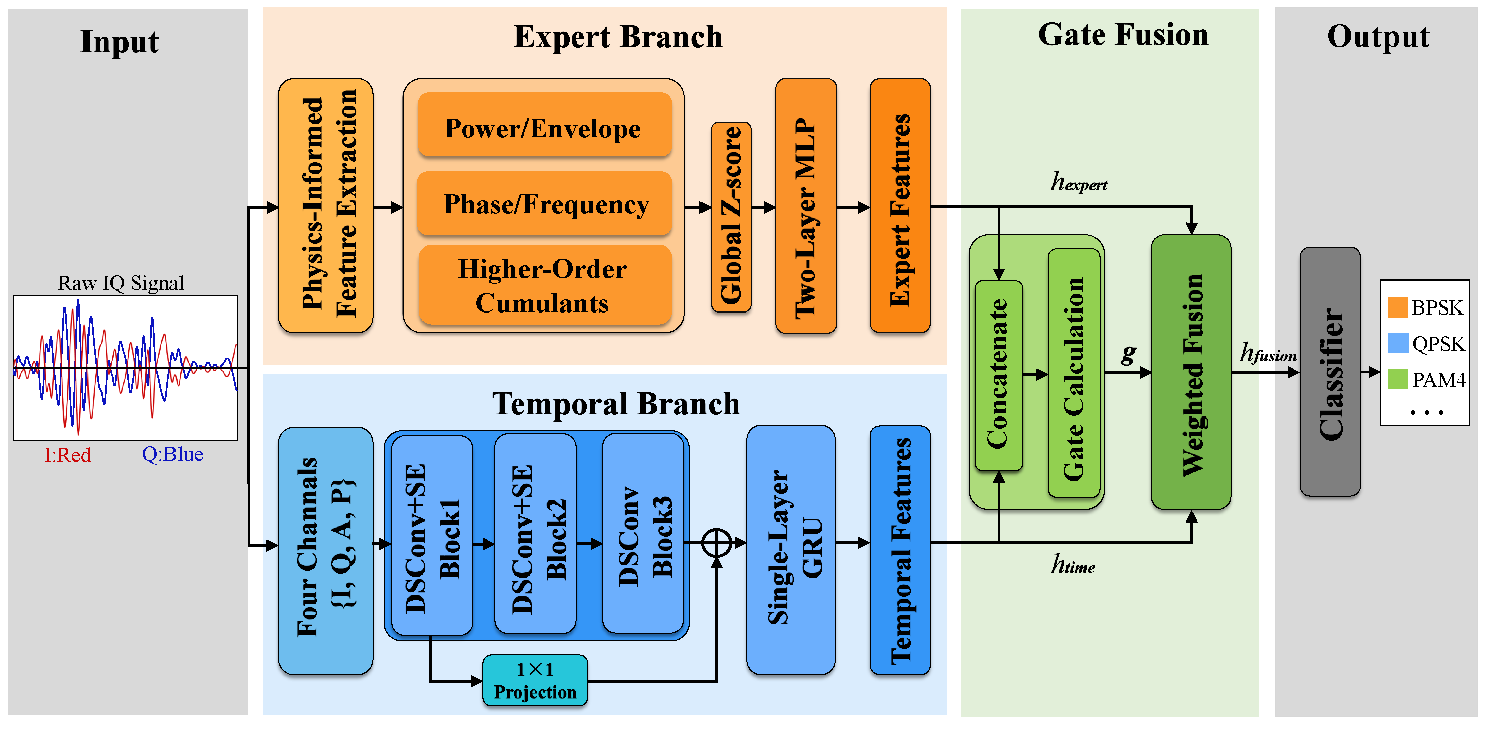
Figure 1. Overall architecture of LGP-Net.
Electronics 15 02261 g001
Figure 2. Classification accuracy versus SNR on RadioML 2016.10A and RadioML 2016.10B.
Electronics 15 02261 g002
Figure 3. Per-class accuracy versus SNR on RadioML 2016.10A.
Electronics 15 02261 g003
Figure 4. Per-class accuracy versus SNR on RadioML 2016.10B.
Electronics 15 02261 g004
Figure 5. Normalised confusion matrices on RadioML 2016.10A (11 classes), shown at + 10 dB, 0 dB, 6 dB, and averaged over all SNRs.
Electronics 15 02261 g005
Figure 6. Normalised confusion matrices on RadioML 2016.10B (10 classes), shown at + 10 dB, 0 dB, 6 dB, and averaged over all SNRs.
Electronics 15 02261 g006
Figure 7. t-SNE visualisation of LGP-Net’s fused representation on RadioML 2016.10A.
Electronics 15 02261 g007
Figure 8. t-SNE visualisation of LGP-Net’s fused representation on RadioML 2016.10B.
Electronics 15 02261 g008
Figure 9. Parameter–accuracy scatter on RadioML 2016.10A. Colored circles denote comparison models, and LGP-Net is marked with a red star.
Electronics 15 02261 g009
Figure 10. Parameter–accuracy scatter on RadioML 2016.10B. Colored circles denote comparison models, and LGP-Net is marked with a red star.
Electronics 15 02261 g010
Figure 11. Per-SNR accuracy for the three major-component ablation variants on RadioML 2016.10A. The gap between Full LGP-Net and each variant widens in the transitional regime around 0 dB.
Electronics 15 02261 g011
Figure 12. Per-SNR accuracy for the three major-component ablation variants on RadioML 2016.10B.
Electronics 15 02261 g012
Figure 13. Per-SNR accuracy of eight expert-group ablation variants on RadioML 2016.10A.
Electronics 15 02261 g013
Figure 14. Overall accuracy of eight expert-group ablation variants on RadioML 2016.10A.
Electronics 15 02261 g014
Figure 15. Per-SNR accuracy for temporal-branch sub-module ablations on RadioML 2016.10A.
Electronics 15 02261 g015
Figure 16. Per-SNR accuracy for different fusion rules on RadioML 2016.10B.
Electronics 15 02261 g016
Figure 17. Per-class recall: full model compared with the fixed-weight variant at SNR = 4 , 0, + 6 dB on RadioML 2016.10B.
Electronics 15 02261 g017
Figure 18. Accuracy versus JSR under controlled co-channel interference on RadioML 2016.10B at 0 dB SNR.
Electronics 15 02261 g018
Figure 19. Gate heatmap (left) and front/back half-dimension mean gate curves (right) versus SNR on RadioML 2016.10A.
Electronics 15 02261 g019
Figure 20. Gate entropy versus SNR on RadioML 2016.10A and RadioML 2016.10B.
Electronics 15 02261 g020
Figure 21. Mean gate value per modulation class versus SNR on RadioML 2016.10A.
Electronics 15 02261 g021
Figure 22. Mean gate value per modulation class versus SNR on RadioML 2016.10B.
Electronics 15 02261 g022
Table 1. Normalisation stages in LGP-Net.
Signal FormNormalisationDownstream Consumer
Raw z [ n ] = I raw + j Q raw noneexpert-feature computation
Four-channel tensor X per-sample Z-score (Equation (2))temporal branch
Expert vector h prior R 11 global Z-scoreexpert branch MLP
Table 2. Notational conventions for signal representations and derived quantities used in Section 3.3.
SymbolExpressionDescriptionRange/Note
z [ n ] I raw [ n ] + j Q raw [ n ] Complex baseband signal n = 0 , , N 1
μ z E [ z ] Signal meanscalar
z ˜ [ n ] z [ n ] μ z Zero-mean signal n = 0 , , N 1
A [ n ] | z [ n ] | Instantaneous amplitude≥0
A ¯ E [ A ] Mean amplitudescalar
A ^ [ n ] A [ n ] / ( A ¯ + ϵ 1 ) Normalised amplitude ϵ 1 = 10 4
ϕ [ n ] arg z [ n ] Instantaneous phase [ π , π )
Δ ϕ [ n ] wrap ϕ [ n + 1 ] ϕ [ n ] Phase difference [ π , π ]
Table 3. Physics-informed expert feature vector (11 dimensions), computed from raw IQ data. G1: power/envelope; G2: phase/instantaneous frequency; G3: higher-order cumulants.
GroupIdxSymbolFormula (Definition)Feature
G10 M 2 E [ | z | 2 ] Mean Power
1 σ a a std ( A ^ ) Normalised Amp. Std
2 κ a E [ A ^ 4 ] / ( E [ A ^ 2 ] ) 2 Amplitude Kurtosis
3 γ max max n A [ n ] / ( A ¯ + ϵ 1 ) Peak Power Ratio
G24 σ Δ ϕ std ( Δ ϕ ) Phase Jitter
5 σ f i std ( f i ) , f i = Δ ϕ / ( 2 π ) Frequency Jitter
6 f i , max max n | f i [ n ] | Peak Freq Deviation
G37 C 4 raw E [ | z | 4 ] | E [ z 2 ] | 2 2 ( E [ | z | 2 ] ) 2 Raw 4th Cumulant
8 | C 20 | | E [ z ˜ 2 ] | 2nd Cumulant Magnitude
9 C 21 E [ | z ˜ | 2 ] 2nd Cumulant Power
10 | C 42 | | E [ | z ˜ | 2 z ˜ 2 ] | E [ z ˜ 2 ] | 2 2 ( E [ | z ˜ | 2 ] ) 2 | 4th Cumulant Magnitude
Table 4. Parameter and MAC breakdown of LGP-Net ( d = 52 ). Total: 39,019 params/2.77 M MACs on RadioML 2016.10A ( C = 11 ); 38,860 params/2.77 M MACs on RadioML 2016.10B ( C = 10 ). Bold entries indicate total parameter and MAC counts.
ModuleParamsMACs
DSConv Block 1 ( 4 20 , k = 7 , SE)27119,128
DSConv Block 2 ( 20 48 , k = 5 , SE)1738148,598
DSConv Block 3 ( 48 d , k = 3 , no SE)2692351,232
Residual projection ( 20 d , 1 × 1 )1040133,120
GRU ( d d , single layer, L = 128 )16,5122,103,296
Temporal Branch subtotal22,2532,755,374
Expert MLP ( 11 144 d + LayerNorm)89489072
Gated Fusion ( 2 d d , linear)54045408
Classification heads ( d C , × 3 ; C = 11 )23881716
Total (2016.10A, C = 11 )39,0192,771,570
Total (2016.10B, C = 10 )38,8602,771,414
Table 5. Dataset comparison: RadioML 2016.10A and RadioML 2016.10B.
Dimension2016.10A2016.10B
Modulation classes1110
Classes8PSK, AM-DSB, AM-SSB, BPSK, CPFSK, GFSK, PAM4, QAM16, QAM64, QPSK, WBFM8PSK, AM-DSB, BPSK, CPFSK, GFSK, PAM4, QAM16, QAM64, QPSK, WBFM
Total samples220,0001,200,000
Samples per class per SNR10006000
Train/Val/Test split132,000/44,000/44,000720,000/240,000/240,000
SNR range 20 to + 18  dB (2 dB step)
Channel conditionsAWGN + multipath fading + SRO + CFO
Notescontains AM-SSBAM-SSB removed
Table 6. Summary of hyperparameters used in all experiments.
CategorySetting
OptimiserAdamW, weight decay 5 × 10 3 , gradient clip 2 = 5.0
Batch size128
Random seed42 for data partitioning and model training
Learning rateLinear warm-up + cosine decay ( T max = 300 , η min = 10 6 )
Early stoppingTolerance 10 4 on validation accuracy
Dropout p = 0.1 (expert MLP), p = 0.3 (classification head)
Focal loss γ = 2.0
Label smoothing ϵ ls = 0.1
Hidden dimension d52
Table 7. Per-SNR accuracy (%): RadioML 2016.10A (11 classes) and RadioML 2016.10B (10 classes).
SNR (dB)2016.10A2016.10B Δ
 −209.5611.56+2.00
 −189.0611.29+2.23
 −1610.9712.76+1.79
 −1413.7916.48+2.69
 −1216.8122.18+5.37
 −1024.3331.74+7.41
 −841.8642.84+0.98
 −658.5057.39−1.11
 −473.3573.77+0.42
 −280.8985.51+4.62
 087.5791.48+3.91
 290.4393.23+2.80
 490.9293.36+2.44
 691.9093.36+1.46
 891.6393.88+2.25
 1091.4493.80+2.36
 1292.0793.44+1.37
 1492.9093.76+0.86
 1691.9794.45+2.48
 1892.7194.76+2.05
Table 8. Comparison with representative AMC methods on RadioML 2016.10A and 2016.10B, predominantly published in 2024–2026. Overall accuracy is the unweighted mean across all 20 SNR levels as reported in each source; parameter counts are as stated by the original authors. Bold entries indicate the results of LGP-Net.
AuthorYearModelParamsDatasetAvg Acc. (%)
Lin et al. [38]2024LSM7 kA36.39
B39.74
Zhang et al. [21]2024MAMCA16.8 MA60.79
B64.05
Wang et al. [22]2024TCN–GRU253 kA61.56
B64.66
Kong et al. [19]2025TCN–Mamba21.7 MA59.12
B62.26
Shao et al. [11]2025IQFormer350 kA64.19
B63.97
Xing et al. [39]2025AWMN440 kA62.39
B64.50
Suman et al. [20]2025DP–DRSN27 kA61.20
B63.78
Zhang et al. [40]2024CNN–BiLSTM–DNN806 kA62.73
B64.76
Wang et al. [41]2024CC–MSNet654 kA62.86
B65.08
El-Haryqy et al. [42]2025ICRNNA790 kA63.24
B65.39
Huo et al. [12]2026SMTrans66 kA63.27
B65.17
Zhang et al. [43]2024MAE–SigNet270 kA63.77
B65.28
Luo et al. [44]2024RLITNN181 kA63.84
B65.32
Zhang et al. [45]2023AMC–Net470 kA62.51
B64.63
Wu et al. [46]2025CBADNN388 kA64.02
B65.50
Zhang et al. [24]2025MLD–Net290 kA61.14
B64.62
Qu et al. [47]2024TLDNN243 kA62.83
Hu et al. [13]2025MFCA–Transformer18.35 MA62.74
Lin et al. [48]2025MMF–GNN∼1 MA63.26
Wang et al. [49]2025CCTL–Net154 kA62.97
Li et al. [50]2024CV–TRN251 kA64.43
Zheng et al. [51]2025SFFN360 kA63.84
Ning et al. [52]2024AbFTNet175 kA64.59
Zhou et al. [53]2026EMST–Net260 kA62.79
LGP-Net (Ours)2026LGP-Net39,019A62.76
38,860B65.00
Table 9. Same-protocol comparison with reimplemented lightweight AMC baselines. Accuracy values are reported in percent. Bold entries indicate the results of LGP-Net.
ModelParams
A
Params
B
Acc.
A
Acc.
B
Mean
Acc.
Mean
0 dB
INT8
(MB)
Peak
(KB)
MCLDNN [15]406,199406,07063.0164.4863.7590.720.3962
SCNN [18]104,13995,94653.5654.2053.8876.600.0964
MCNet [16]82,05981,54656.3662.1559.2683.140.0864
PET-CGDNN [17]71,87171,74261.3064.7363.0189.580.0758
DAE [6]14,98914,97259.1664.2161.6886.720.0116
ULCNN [14]10,40310,37060.0963.0761.5887.370.0116
LGP-Net39,01938,86062.7665.0063.8889.530.0426
Table 10. Hardware efficiency profile of LGP-Net. CPU latency was measured on Intel Core Ultra 7 155H with a single CPU thread and no discrete GPU. CUDA latency was measured on NVIDIA RTX 3090. The INT8 storage follows a one-byte-per-parameter estimate.
Metric2016.10A ( C = 11 )2016.10B ( C = 10 )
Parameters39,01938,860
MACs/FLOPs2.77 M/5.54 M2.77 M/5.54 M
FP32 model size152.42 KB151.80 KB
Estimated INT8 parameter storage0.04 MB0.04 MB
Peak activation memory26.00 KB26.00 KB
Total inference memory (FP32)178.42 KB177.80 KB
CPU latency (batch = 1)4.09 ms4.09 ms
CPU latency (batch = 128, per sample)228  μ s229  μ s
CUDA latency (batch = 1)1.15 ms1.15 ms
CUDA latency (batch = 128, per sample)9.3  μ s9.7  μ s
Table 11. Post-training quantisation and export probes of LGP-Net.
ProbeAccuracy/AgreementArtifact/Graph Result
Dynamic INT8 PTQ (2016.10A)62.76%→62.66% ( 0.10  pp)169.39 KiB→79.65 KiB
Dynamic INT8 PTQ (2016.10B)65.00%→64.56% ( 0.44  pp)168.83 KiB→79.65 KiB
TorchScript tracing100.00% top-1 agreementmax logit difference < 10 5
Unrolled FP32 TFLite100.00% top-1 agreement598.4 KB; no WHILE/Flex
Unrolled dynamic-range TFLite99.90% top-1 agreement504.9 KB; no WHILE/Flex
Table 12. Major-component ablation on RadioML 2016.10A and RadioML 2016.10B: overall and selected per-SNR accuracy of the four variants. Bold entries indicate the Full LGP-Net results.
VariantRadioML 2016.10ARadioML 2016.10B
Overall −6 dB 0 dB +10 dB Overall −6 dB 0 dB +10 dB
Full LGP-Net62.7658.5087.5791.4465.0057.3991.4893.80
w/o Expert Branch53.3546.2571.5879.8461.2645.2882.6892.03
w/o Temporal Branch29.2531.3440.9936.3823.6225.3628.4431.09
w/o Gating58.5253.9780.7188.1757.5051.2375.1486.63
Table 13. Sub-module ablation of the temporal branch on RadioML 2016.10A. Bold entries indicate the Full LGP-Net results.
VariantOverall (%)−6 dB (%)0 dB (%)+10 dB (%)
Full LGP-Net62.7658.5087.5791.44
LGP-Net (w/o SE)29.2721.8435.5644.59
LGP-Net (w/o GRU)28.0023.1737.2643.00
LGP-Net (w/o SE+GRU)20.3115.8925.7728.00
Table 14. Fusion-rule comparison on RadioML 2016.10B. Accuracy values are reported in percentage points. Bold entries indicate the proposed gated-fusion result.
VariantFusion RuleOverall
(%)
0 dB
(%)
+10 dB
(%)
Transition
(%)
Gain over
Fixed (%)
Full LGP-NetPer-dim adaptive65.0091.4893.8077.04+7.50
Concat-MLPFeature-level nonlinear63.7989.8793.3773.56+6.29
Scalar GateSample-wise scalar62.6887.5392.2071.54+5.18
Fixed 50/50Fixed scalar57.5075.1486.6360.45+0.00
Table 15. Accuracy (%) under controlled co-channel interference on RadioML 2016.10B at 0 dB SNR. Bold entries indicate the Full LGP-Net results.
VariantCleanJSR (dB)
−10 −5 0 +5 +10
Full LGP-Net91.4571.8360.6849.0832.4020.00
LGP-Net (w/o Expert)86.6865.9555.1441.7827.2214.37
LGP-Net (w/o Gating)75.2249.5244.7239.1827.6616.69
Table 16. Gate entropy summary across SNR regimes.
Dataset r ( g ¯ , SNR ) Low H g Mid H g High H g
RadioML 2016.10A0.7100.4700.2880.249
RadioML 2016.10B0.8930.4610.3070.253
Disclaimer/Publisher’s Note: The statements, opinions and data contained in all publications are solely those of the individual author(s) and contributor(s) and not of MDPI and/or the editor(s). MDPI and/or the editor(s) disclaim responsibility for any injury to people or property resulting from any ideas, methods, instructions or products referred to in the content.