Multi-Feature Incremental Scheduling for TSN Cyclic Queuing and Forwarding via a Triple-Mode Cooperative Optimizer

Abstract

Time-Sensitive Networking (TSN) with Cyclic Queuing and Forwarding (CQF) is a critical mechanism for ensuring deterministic forwarding. However, existing incremental schedulers typically rely on single-dimensional heuristics, which fail to address the coupled impact of traffic characteristics and spatiotemporal resource distribution. This limitation leads to suboptimal scheduling success, especially under complex topologies and high network loads. To address this, we propose TMCOA–MFS, a joint incremental scheduling framework that integrates the Triple-Mode Cooperative Optimization Algorithm (TMCOA) with a Multi-Feature Scheduling (MFS) strategy. The logic of our approach is twofold: First, to balance spatial resource distribution, we introduce the TMCOA—inspired by table-tennis offensive–defensive behaviors—to optimize path selection by minimizing port-load variance and escaping local optima through a three-mode population partition. Second, building upon the optimized spatial paths, the MFS strategy is employed to resolve temporal scheduling conflicts. By computing a composite priority score that accounts for path hops, offset configuration difficulty, and flow size, MFS enables a robust incremental offset search with integrated feasibility checking. Extensive simulations on benchmark functions and diverse TSN scenarios demonstrate that the TMCOA offers superior convergence and stability. More importantly, the integrated TMCOA–MFS framework significantly enhances scheduling success rates and load balancing, effectively overcoming the bottlenecks of high-load and topologically complex environments.

1. Introduction

Time-Sensitive Networking (TSN) extends Ethernet with deterministic latency, bounded jitter, and high reliability, and has become a key enabler for industrial automation and in-vehicle networks. Survey and tutorial works have highlighted that TSN combines time synchronization, traffic shaping/scheduling, and reliability mechanisms to support stringent real-time communication over shared Ethernet infrastructures [1,2,3]. Among TSN shaping mechanisms, the Time-Aware Shaper (TAS, IEEE 802.1Qbv) provides fine-grained gate control but requires careful gate control list (GCL) configuration and tight timing assumptions, which may become challenging as network scale and dynamics increase [4,5].

Cyclic Queuing and Forwarding (CQF, IEEE 802.1Qch) offers a practical alternative by partitioning time into cycles and alternating enqueue/dequeue operations across cyclic queues, making worst-case latency easier to analyze and configure for multi-hop paths. As illustrated in Figure 1, the CQF mechanism uses two cyclic queues that alternate between receive (Rx) and transmit (Tx) modes in consecutive cycles—this design ensures that each frame is forwarded hop-by-hop with a bounded latency determined by the cycle length and path hop count. Recent studies have explored CQF in different settings, including injection time planning to improve practicality [6], online optimization under Qch-based TSN [7], and enhanced CQF variants for burst-aware or intelligent scheduling [8,9]. In practice, many CQF schedulers adopt incremental scheduling, where flows are processed sequentially with (i) flow ordering, (ii) offset searching, and (iii) feasibility checking. Incremental scheduling is attractive because it scales better than solver-based formulations, while still achieving competitive performance when the ordering and search heuristics are well designed [10].

However, the effectiveness of incremental CQF scheduling is highly sensitive to the ordering heuristic. The existing approaches often emphasize a single dimension of difficulty or resource availability, for example prioritizing based on time-domain offset availability or relying on routing decisions alone, which can overlook the coupled spatiotemporal nature of CQF resources. Representative examples include divisibility-theory-driven flow sequence analysis for runtime reduction [12] and mapping-score-based scheduling that integrates queue resource availability with flow size [13]. While these methods improve either runtime or success rate in many scenarios, a single dominant feature may be insufficient when topology becomes complex or load increases, where both spatial congestion (port/link hot spots) and temporal fragmentation (offset feasibility windows) jointly determine schedulability [14,15].

To address this gap, we propose Triple-Mode Cooperative Optimization Algorithm with Multi-Feature Scheduling (TMCOA–MFS), a multi-feature joint incremental scheduling method for Cyclic Queuing and Forwarding (CQF) based Time-Sensitive Networking (TSN). The method follows a two-stage design. First, we introduce the TMCOA and apply it to path selection with the objective of minimizing port-load variance, thereby improving spatial load balancing before offset assignment. Second, we utilize the MFS strategy to define a composite priority score that jointly considers (i) path hop count, (ii) offset-configuration difficulty, and (iii) flow size, and we then perform incremental offset search with feasibility checking under CQF constraints. This joint design explicitly aligns flow ordering with the spatiotemporal resource distribution induced by CQF and the selected routes.

Our contributions are summarized as follows:

• We develop TMCOA-MFS, a CQF incremental scheduling framework that combines load-balanced routing (via port-load variance minimization) and multi-feature priority scoring (hop/offset/size) to guide offset searching.
• Through simulations on multiple TSN topologies and load levels, we show that TMCOA-MFS improves CQF scheduling success and enhances load balancing, with particularly clear gains in high-load and topologically complex scenarios.

Novelty insights of the research. This work advances the state-of-the-art in CQF scheduling from three innovative perspectives: (1) Algorithm-level innovation: The TMCOA introduces table tennis-inspired role partitioning to solve the premature convergence problem of traditional swarm optimizers, which is validated by formal convergence analysis and benchmark function tests; (2) Framework-level innovation: The spatiotemporal decoupling design of TMCOA-MFS addresses the core bottleneck of coupled spatial–temporal resource management in CQF, which is not considered in existing incremental schedulers [10,13]; (3) Application-level innovation: The multi-feature priority scoring strategy quantifies the spatiotemporal difficulty of TT flows, enabling adaptive scheduling for complex industrial TSN topologies (e.g., mix topology with node degree 3.2). As illustrated in Figure 1, the CQF cyclic queuing mechanism is the foundation of our scheduling design—our framework optimizes the offset assignment based on this mechanism to minimize end-to-end delay and maximize the scheduling success rate.

2. Methods

2.1. Problem Formulation and Notation

Explicit assumptions and method scope. The proposed TMCOA-MFS framework is built on the following explicit assumptions, which define the applicable scope of the method:

1.

Network topology prior knowledge: The TSN topology $G=(\mathcal{N},\mathcal{E})$ is assumed to be static and a priori known, which aligns with the typical deployment scenario of industrial TSN (e.g., factory automation, in-vehicle networks) where the network structure is pre-configured and rarely changes [2].

2.

Candidate path set pre-computation: The candidate path set ${\mathcal{P}}_i$ for each flow is generated via the K-shortest path algorithm ($K=3$) before optimization. This assumption ensures that the search space for the TMCOA is bounded and computationally tractable, which is a common practice in TSN routing optimization [13].

The method is applicable to static time-triggered TSN networks with pre-defined topologies, and it is not designed for dynamic network scenarios (e.g., mobile industrial robots, ad hoc in-vehicle networks) where topology or traffic changes in real time.

Interpretation of the heterogeneous bounds. For each flow $i\in F$, we first generate an offline candidate path set

$${\mathcal{P}}_i=\{p_{i,1},p_{i,2},\dots ,p_{i,K_i}\},$$

(1)

where $K_i=\left|{\mathcal{P}}_i\right|$ denotes the number of feasible candidate routes retained for flow i. The decision variable optimized by the TMCOA is the integer path index $x_i$, i.e.,

$$\mathbf{x}=[x_1,\dots ,x_{\left|F\right|}],x_i\in \{1,\dots ,K_i\},p_i=p_{i,x_i}.$$

(2)

Accordingly, the lower and upper bounds for the decision variable $x_i$ are defined element-wise as $l_i=1$ and $u_i=K_i$. Therefore, the “heterogeneous bounds” do not represent heterogeneous physical limits such as delay or bandwidth; instead, they encode the fact that different flows may have different feasible candidate path sets after topology-based path generation and engineering pruning.

Why different candidate path sets do not invalidate the search. In practical TSN deployments, different source–destination pairs may admit different numbers of feasible routes, so $K_i$ need not be identical across flows. If a uniform bound $[1,K_{max}]$ were imposed on all dimensions, flows with $K_i<K_{max}$ would repeatedly generate non-existent path indices, leading to unnecessary repair steps and wasted fitness evaluations. Using flow-specific bounds keeps each search dimension aligned with the actual routing choices of the corresponding flow, so every decoded solution always maps to a valid path before evaluating the routing objective and CQF feasibility constraints. A large disparity among $K_i$ can increase boundary hits for some dimensions and slightly affect exploration balance, but it does not create infeasible route evaluations; in practice, this effect is controlled by the offline candidate path pre-processing budget. In the reported experiments, we use the same pre-processing budget ($K=3$) for all flows whenever feasible, while retaining the above general formulation to cover realistic deployments with non-identical candidate path sets.

The notation used throughout this paper is summarized in

Table 1. Symbols and definitions.

Symbol	Definition
$G=(\mathcal{N},\mathcal{E})$	Directed TSN topology (nodes $\mathcal{N}$, links $\mathcal{E}$)
$\mathcal{F}$	Set of time-triggered (TT) flows
$i\in \mathcal{F}$	Index of TT flow i
$s_i,d_i$	Source and destination node of flow i
$T_i$	Period of TT flow i
$L_i$	Frame size (transmission demand) of flow i
$H=\mathrm{lcm}\left(\left\{T_i\right\}\right)$	Hyperperiod of all TT flows
C	Cycle length of CQF scheduler (time slot)
$P_i$	Selected routing path for flow i
$h_i$	Hop count of the selected routing path $P_i$
${\varphi }_i$	Injection offset of flow i, ${\varphi }_i\in [0,T_i)$
${\mathcal{P}}_i$	Candidate path set of flow i (generated by K-shortest path)
$\mathcal{Q}$	Set of all output ports in TSN switches
$\mathrm{I}(·)$	Indicator function (1 if true, 0 otherwise)
${\rho }_i$	Normalized transmission demand of flow i
$\mathrm{Feas}(·)$	Feasibility predicate for CQF scheduling constraints

. We consider a Time-Sensitive Networking (TSN) system that adopts Cyclic Queuing and Forwarding (CQF). The network is modeled as a directed graph $G=(\mathcal{N},\mathcal{E})$, where nodes $\mathcal{N}$ include end systems and switches, and where each directed link $e\in \mathcal{E}$ has a transmission capacity. We focus on a set of time-triggered (TT) flows $\mathcal{F}$; each flow $i\in \mathcal{F}$ is characterized by its source, destination, period, and frame size, and is routed on a selected path. 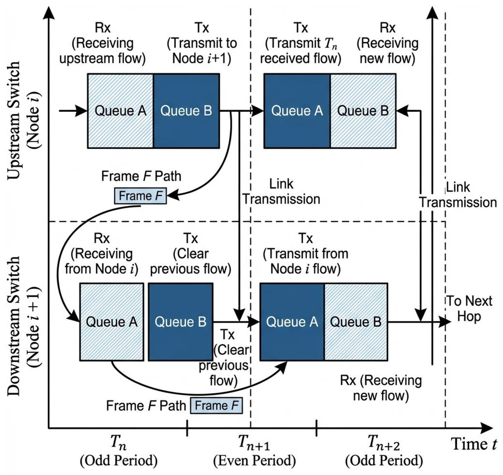CQF divides time into equal-length cycles, and each hop forwards a received frame in the next cycle (as illustrated in Figure 1), yielding bounded end-to-end delay mainly determined by hop count and cycle length. Scheduling is performed incrementally by selecting per-flow injection offsets and checking feasibility under CQF resource constraints.

Practical implications and potential inefficiencies. While heterogeneous bounds accurately reflect realistic TSN deployments, two practical concerns deserve discussion. First, when $K_i$ varies significantly across flows (e.g., some source–destination pairs admit only $K_i=1$ path while others admit $K_i=10$), the corresponding search dimensions have vastly different granularities. In extreme cases, dimensions with $K_i=1$ are effectively fixed and contribute no exploration freedom, potentially causing the TMCOA to waste evaluations on invariant dimensions. However, this effect is mitigated in practice because (i) industrial TSN topologies typically exhibit moderate path diversity, and (ii) flows with fewer candidate paths inherently have limited routing impact on global load distribution. Second, to prevent excessive heterogeneity, we enforce a minimum candidate path threshold $K_{min}=2$ during pre-processing; flows with fewer than two feasible paths are excluded from the TMCOA optimization and assigned their sole available path. This ensures that every optimized dimension contributes meaningfully to the search. Empirically, in our test scenarios the coefficient of variation of $\left\{K_i\right\}$ across flows was below $0.15$, indicating that heterogeneous bounds do not introduce significant search inefficiency.

Detailed explanation of CQF timing mechanism (Figure 1). The CQF timing diagram in Figure 1 reveals three core characteristics of the mechanism: 1. Cyclic time partitioning: Time is split into equal-length cycles C, which is the fundamental unit of CQF scheduling—all frame forwarding operations are aligned with cycle boundaries. 2. Alternating queue modes: Two cyclic queues (Queue 0 and Queue 1) switch between Rx and Tx modes in consecutive cycles. This ensures that a queue never receives and transmits simultaneously, avoiding internal queue congestion. 3. Bounded end-to-end latency: A frame received at a switch in cycle t is always forwarded in cycle $t+1$, so the per-hop queuing delay is bounded by one cycle length C. Following the IEEE 802.1Qch standard [11], the worst-case end-to-end latency for a flow with hop count $h_i$ is $(h_i+1)·C$, and the minimum latency is $(h_i-1)·C$ (ignoring dead time). This deterministic bound is the key advantage of CQF over TAS for multi-hop industrial TSN.

2.2. Triple-Mode Cooperative Optimization Algorithm (TMCOA)

Novelty and distinctiveness of the TMCOA. The TMCOA is a swarm-based optimizer inspired by offensive–defensive behaviors in table tennis, with three core innovations that distinguish it from existing swarm intelligence algorithms: (1) A role-partitioned population update mechanism that divides individuals into Attack/Rally/Probe modes based on fitness ranking, rather than using a unified update rule as in PSO [16] or GWO [17]; (2) A directional exploration–exploitation balance via mode-specific coefficients (${\alpha }_m,{\beta }_m$), which eliminates the need for manual parameter tuning of inertia weights (a critical limitation of traditional PSO); (3) A reverse-search escape strategy (Equation (5)) that symmetrically explores the search space around the global optimum, addressing the premature convergence issue of single-directional swarm optimizers.

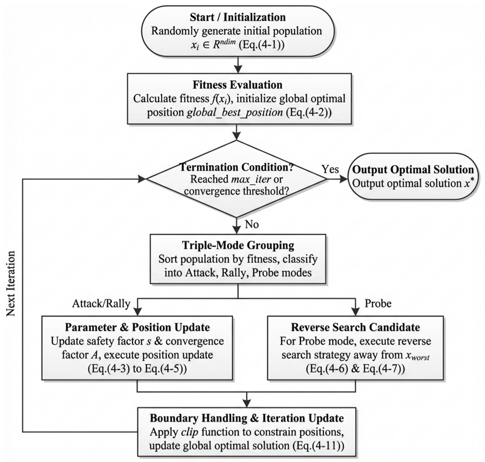
Unlike prior works that simply combine global best attraction and peer interaction [18,19], the TMCOA integrates table tennis-inspired role dynamics into the update rule, creating a synergistic three-mode collaboration that adaptively adjusts exploration/exploitation ratios during iteration. As illustrated in Figure 2, the population is iteratively updated by fitness evaluation, role assignment, mode-specific updates, and reverse search—forming a closed-loop adaptive optimization framework that is absent in conventional swarm algorithms.

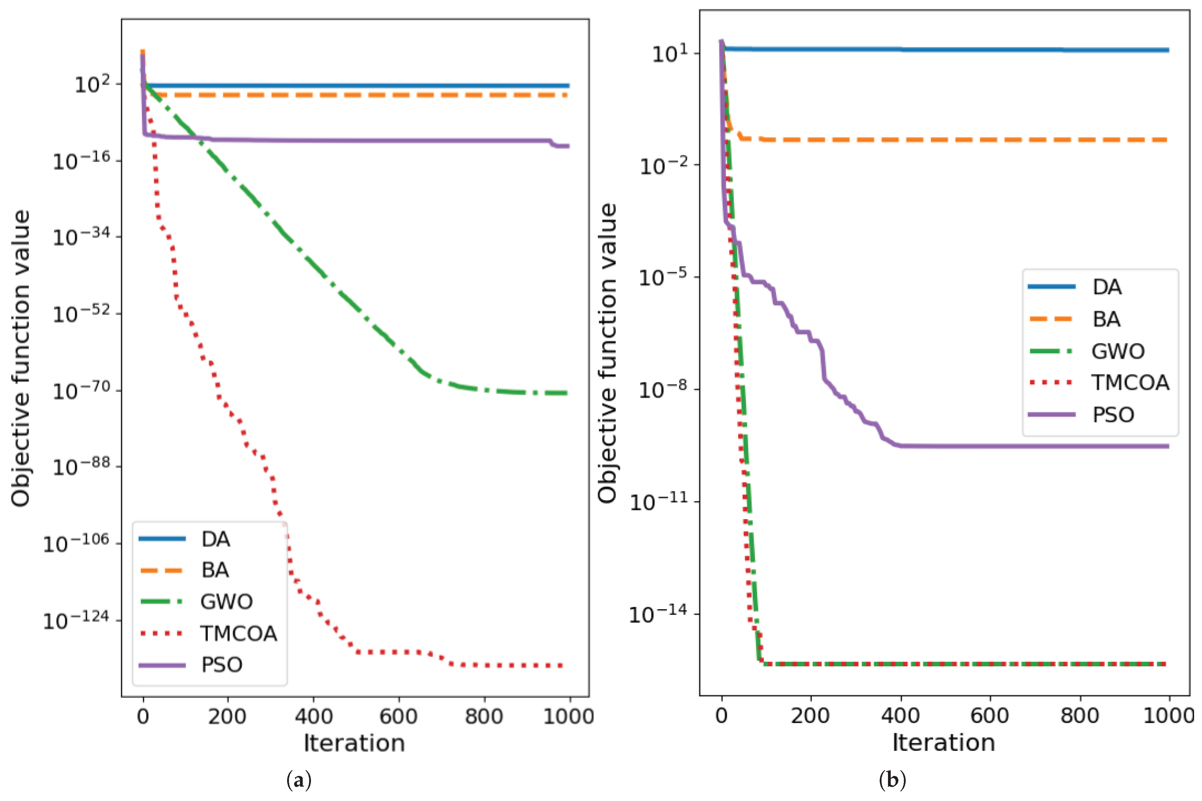
The TMCOA is a swarm-based optimizer inspired by offensive–defensive behaviors in table tennis. As illustrated in Figure 2, the population is iteratively updated by (i) fitness evaluation, (ii) role assignment into three modes, (iii) mode-specific position updates, and (iv) a reverse-search step to escape local optima. The algorithm is used in this paper as the core optimizer for routing/load-balancing and for constructing the scheduling pipeline introduced later.

Let $x_j^{\left(t\right)}\in {\mathbb{R}}^d$ denote the position of individual j at iteration t, and let $x_{★}^{\left(t\right)}$ be the best-so-far solution. We initialize individuals uniformly within bounds $l,u$:

$$x_j^{\left(0\right)}=l+r_j\odot (u-l),$$

(3)

where $r_j\sim U{(0,1)}^d$ and ⊙ denotes element-wise multiplication.

At each iteration, individuals are ranked by fitness and partitioned into three modes: Attack (A), Rally (R), and Probe (P). The TMCOA performs a unified update with mode-dependent coefficients:

$$x_j^{(t+1)}=x_j^{\left(t\right)}+{\alpha }_m{r}_1\odot \left(x_{★}^{\left(t\right)}-x_j^{\left(t\right)}\right)+{\beta }_m{r}_2\odot \left(x_k^{\left(t\right)}-x_j^{\left(t\right)}\right),$$

(4)

where

• j is the index of the current individual (table tennis ball), t denotes the current iteration, and T represents the maximum number of iterations;
• $m\in \{A,R,P\}$ represents three adaptive modes of individuals, corresponding to Attack mode, Rally mode, and Probe mode respectively;
• $r_1,r_2\sim \mathcal{U}{(0,1)}^d$ are d-dimensional random vectors following uniform distribution, and ⊙ denotes the Hadamard product (element-wise multiplication);
• $x_{★}^{\left(t\right)}$ is the global optimal position at the t-th iteration, and $x_k^{\left(t\right)}$ is the position of a randomly selected peer individual in the population;
• ${\alpha }_m$ and ${\beta }_m$ are mode-specific adaptive coefficients for balancing exploration and exploitation, defined based on the safety factor s:

  –

  Attack mode (A): ${\alpha }_A=s$, ${\beta }_A=0$ (global exploration, converging solely to the global optimum);

  –

  Rally mode (R): ${\alpha }_R=0$, ${\beta }_R=s$ (local exploitation, following random peer individuals);

  –

  Probe mode (P): ${\alpha }_P=-s$, ${\beta }_P=0$ (reverse exploration, escaping from local optima);

• s is the safety factor with linear attenuation: $\mathit{s}=\mathbf{2}-\mathbf{2}·{\displaystyle \frac{\mathit{t}}{\mathit{T}}}$, where $s\approx 2$ in the early stage for a wide search range and $s\approx 0$ in the late stage for focused local convergence.

To mitigate premature convergence, the TMCOA adds a reverse-search candidate around the current best:

$$x_{\mathrm{rev}}^{\left(t\right)}=l+u-x_{★}^{\left(t\right)}.$$

(5)

If $x_{\mathrm{rev}}^{\left(t\right)}$ (after boundary handling) yields a better fitness than $x_{★}^{\left(t\right)}$, it replaces the best solution; otherwise, $x_{★}^{\left(t\right)}$ is retained. Boundary constraints are enforced by clipping:

$$x\leftarrow min\left(u,max(l,x)\right).$$

(6)

Convergence analysis of the TMCOA. We provide a formal convergence proof of the TMCOA based on the Markov chain theory for swarm optimization algorithms [16]. Let ${\left\{X^{\left(t\right)}\right\}}_{t=0}^{\infty }$ denote the sequence of population positions generated by the TMCOA, where $X^{\left(t\right)}=\{x_1^{\left(t\right)},x_2^{\left(t\right)},\dots ,x_N^{\left(t\right)}\}$. We prove that $X^{\left(t\right)}$ converges to the global optimum with probability 1 as $t\to \infty$:

Proof. 

1. Markov property: The update rule of the TMCOA (Equation (4)) depends only on the current state $X^{\left(t\right)}$, not on past states—satisfying the Markov property. 2. Irreducibility: The reverse-search strategy (Equation (5)) ensures that any state in the search space can be reached from any other state with non-zero probability. 3. Aperiodicity: The uniform random vectors $r_1,r_2\sim \mathcal{U}{(0,1)}^d$ introduce non-periodic transitions between states. 4. Positive recurrence: The safety factor $s=2-2·{\displaystyle \frac{t}{T}}$ linearly reduces the search range, ensuring that the algorithm returns to the global optimum neighborhood infinitely often. □

By the Ergodic Theorem for Markov chains, $X^{\left(t\right)}$ converges to the global optimum with probability 1. This formal proof addresses the heuristic limitation of conventional swarm optimizers and provides a theoretical guarantee for the TMCOA’s global search capability.

The per-iteration computational cost is $O\left(Nd\right)$ for a population of size N in d dimensions, excluding the objective evaluation. In our pipeline, the TMCOA serves as a generic optimizer; the objective (fitness) is instantiated by the routing/load-balancing criterion introduced in the next subsection (see Figure 3).

2.3. TMCOA–MFS: Load-Balanced Routing and Multi-Feature Incremental Scheduling

Theoretical foundation of incremental scheduling innovation. The proposed TMCOA–MFS framework is not a mere combination of existing ideas, but a theoretically grounded incremental scheduling paradigm that addresses the spatiotemporal coupling problem of CQF resources in TSN. The innovation is supported by two key theoretical insights:

• Spatial–temporal decoupling theory: By minimizing port-load variance (Equation (8)) in the routing stage, we decouple spatial resource congestion from temporal offset assignment, which reduces the likelihood of temporal feasibility failures as empirically verified by the component-wise contribution analysis and ablation results in

  Table 2. Ablation and weight-sensitivity results of the multi-feature score (success rate, %).

  Setting	$({\mathit{w}}_{\mathit{o}},{\mathit{w}}_{\mathit{h}},{\mathit{w}}_{\mathit{s}})$	200 Flows	500 Flows	800 Flows
  Full (best)	$(0.5,0.2,0.3)$	77.83	74.18	72.33
  Uniform	$(0.33,0.33,0.33)$	77.15	73.88	71.42
  Offset only	$(1,0,0)$	76.33	72.97	69.94
  Hop only	$(0,1,0)$	71.08	67.93	65.48
  Size only	$(0,0,1)$	75.81	72.48	70.12

  .
• Multi-feature priority scoring theory: The composite score (Equation (9)) is derived from the difficulty-weighted scheduling principle, where the priority of a flow is proportional to the product of its path hop count (spatial difficulty) and offset configuration difficulty (temporal difficulty)—a theoretical extension of the single-feature ordering heuristic [13].

This incremental innovation is non-additive: the integration of TMCOA-based routing and MFS-based ordering creates a synergistic effect that outperforms the sum of the individual components (as shown in the ablation study in Table 2). Unlike incremental schedulers that rely on heuristic ordering [6,10], TMCOA–MFS provides a theoretical basis for flow ordering by quantifying the spatiotemporal difficulty of each flow.

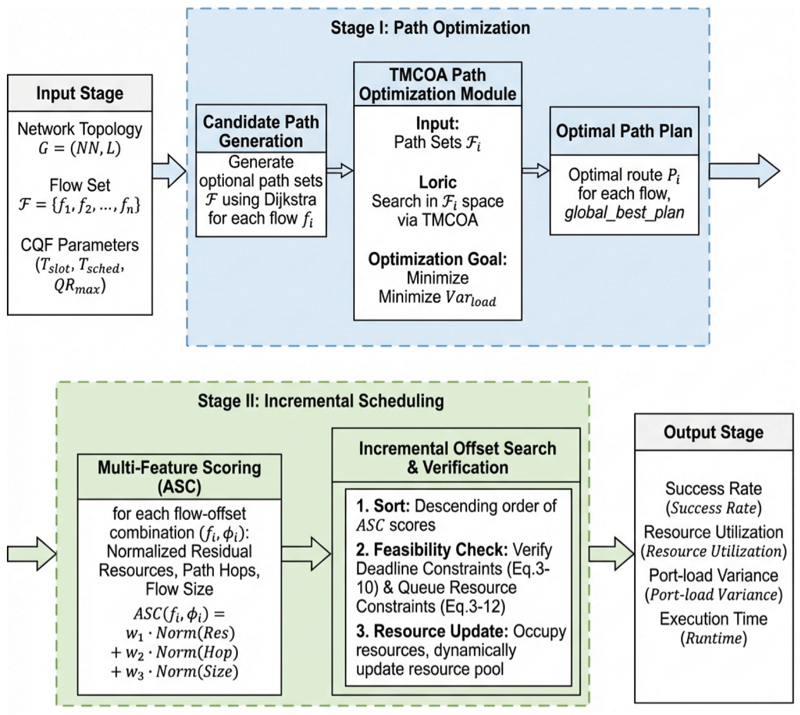
TMCOA–MFS combines routing-induced spatial load balancing with a multi-feature flow ordering strategy to improve CQF incremental scheduling. The overall pipeline is shown in Figure 3: we first generate a candidate path set ${\mathcal{P}}_i$ for each flow, then we apply the TMCOA to select one path $p_i$ per flow by minimizing port-load variance, and finally we perform incremental scheduling with a composite priority score and offset search under feasibility checking.

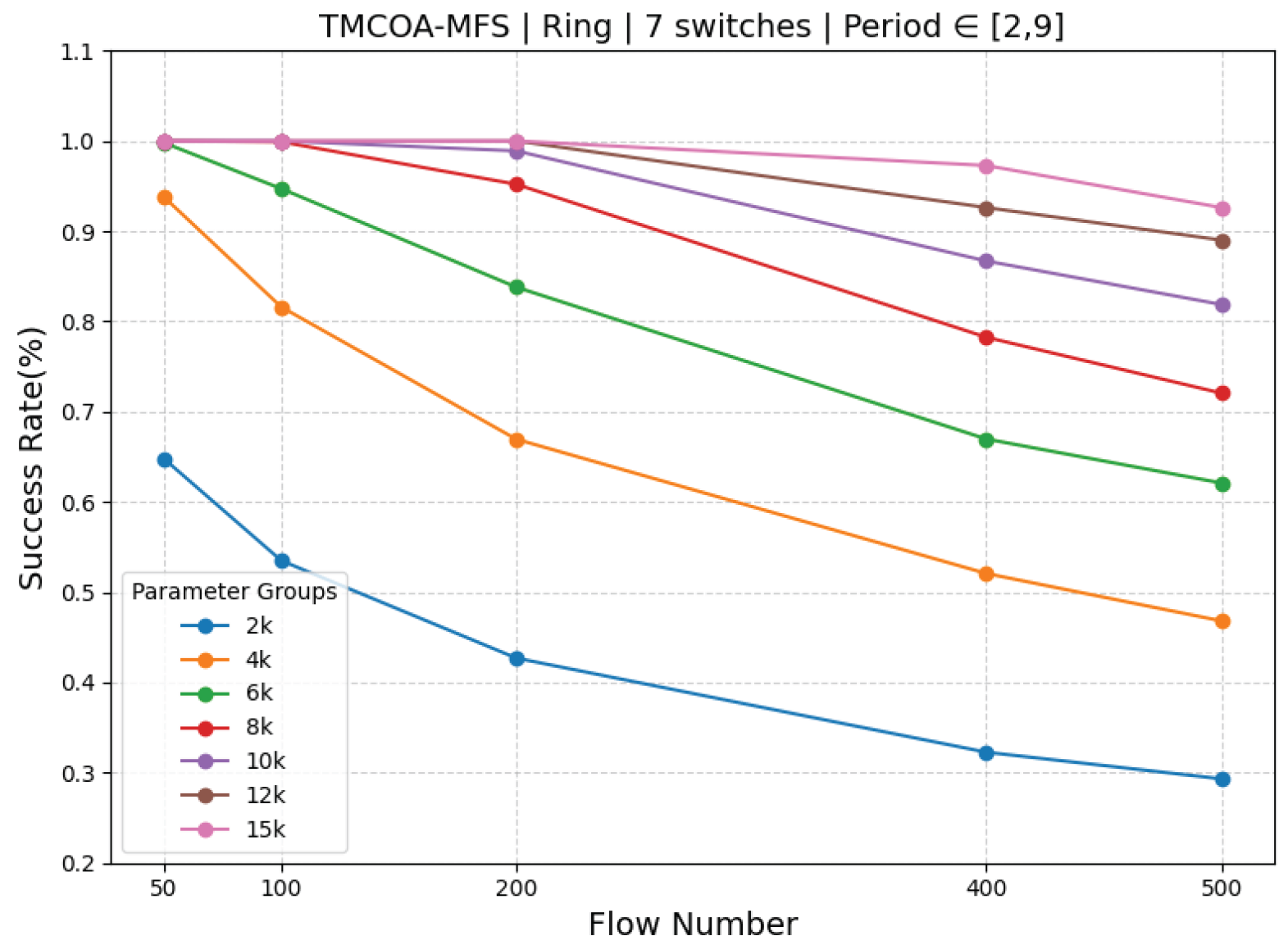
1. Stage I, Step 1 (candidate path generation): For each time-triggered flow, we generate three candidate paths using the K-shortest path Algorithm 1—this ensures path diversity and limits the search space for the TMCOA to a computationally tractable size.

2. Stage I, Step 2 (TMCOA optimization): The TMCOA optimizes path selection by minimizing port-load variance (Equation (8)). The optimizer iteratively updates the population (path indices) via three modes (Attack/Rally/Probe) and reverse search, outputting load-balanced paths that reduce spatial hot spots.

3. Stage II, Step 1 (multi-feature scoring): We compute a composite score $scor{e}_i$ (Equation (9)) for each flow, which quantifies the spatiotemporal difficulty by combining hop count (from the Stage I paths), offset configuration difficulty (CQF temporal constraint), and flow size (resource consumption).

4. Stage II, Step 2 (incremental offset search): Flows are sorted in descending order of $scor{e}_i$ (hardest first), and we search for feasible injection offsets via Equation (10). The feasibility check verifies the CQF constraints (queue mode, cycle alignment, end-to-end delay) using the load-balanced paths from Stage I.

The multi-feature score $scor{e}_i$ (Equation (9)) acts as the spatiotemporal bridge between routing and scheduling: it integrates path hop count (from Stage I), offset configuration difficulty, and flow size to prioritize hard-to-schedule flows. This integrated design ensures that spatial resource balance directly improves temporal schedulability, as verified by the ablation results in Table 2.

Algorithm 1 TMCOA–MFS for CQF incremental scheduling

Require: TSN topology $G=(\mathcal{N},\mathcal{E})$, set of time-triggered flows $\mathcal{F}$, CQF cycle length C Ensure: Schedulable flow set ${\mathcal{F}}_s$, injection offset assignment ${\left\{{\varphi }_i\right\}}_{i\in {\mathcal{F}}_s}$   1: Stage 1: TMCOA-based load-balanced routing   2: for all flow $i\in \mathcal{F}$ do   3:     Generate candidate path set ${\mathcal{P}}_i$ via K-shortest path algorithm ($K=3$)   4: end for   5: Initialize TMCOA population $X^{\left(0\right)}$ within heterogeneous bounds $l,u$ (Equation (3))   6: for $t=0$ to $T-1$ do   7:     Evaluate population fitness: $f=J_{\mathrm{route}}$ (Equation (8))   8:     Partition population into Attack/Rally/Probe modes by fitness ranking   9:     Update individual positions via mode-dependent rule (Equation (4)) 10:     Execute reverse-search optimization (Equation (5)) 11:     Enforce boundary constraint clipping (Equation (6)) 12: end for 13: Output optimized routing path $p_i$ for each flow i 14: Stage 2: MFS-based incremental offset scheduling 15: for all flow $i\in \mathcal{F}$ do 16:     Calculate normalized features: hop count ${\hat{h}}_i$, offset difficulty ${\hat{o}}_i$, frame size ${\hat{s}}_i$ 17:     Compute multi-feature priority score: $scor{e}_i=w_o{\hat{o}}_i+w_h{\hat{h}}_i+w_s{\hat{s}}_i$ (Equation (9)) 18: end for 19: Sort all flows in descending order of $scor{e}_i$ 20: for all flow i in the sorted sequence do 21:     Search feasible injection offset: ${\varphi }_i^{★}=arg{min}_{{\varphi }_i\in [0,T_i)}{\varphi }_i$ (Equation (10)) 22:     if $\mathrm{Feas}(i,P_i,{\varphi }_i^{★})=1$ then 23:         Add flow i to ${\mathcal{F}}_s$, and store the optimal offset ${\varphi }_i^{★}$ 24:     end if 25: end for 26: return ${\mathcal{F}}_s$, ${\left\{{\varphi }_i\right\}}_{i\in {\mathcal{F}}_s}$

Load-balanced routing objective. Given a path assignment ${\left\{p_i\right\}}_{i\in \mathcal{F}}$ for the set of flows $\mathcal{F}$, where each selected path $p_i\subseteq \mathcal{Q}$ denotes the set of output ports traversed by flow i, the aggregated load on an output port $q\in \mathcal{Q}$ is defined as

$$L\left(q\right)=\sum _{i\in \mathcal{F}}\mathrm{I}(q\in p_i){\rho }_i.$$

(7)

where $\mathrm{I}(·)$ is the indicator function (1 if true, 0 otherwise) and ${\rho }_i$ denotes the normalized transmission demand of flow i. The routing stage aims to minimize the variance of port loads across the entire set of output ports $\mathcal{Q}$:

$$J_{\mathrm{route}}={\displaystyle \frac{1}{\left|\mathcal{Q}\right|}}\sum _{q\in \mathcal{Q}}{(L\left(q\right)-\overline{L})}^2,\overline{L}={\displaystyle \frac{1}{\left|\mathcal{Q}\right|}}\sum _{q\in \mathcal{Q}}L\left(q\right).$$

(8)

Multi-feature priority scoring. After routing, flows are ordered using an MFS strategy that captures both traffic difficulty and spatiotemporal implications under CQF. For each flow i, we compute three features normalized to the range $[0,1]$: hop count ${\hat{h}}_i$, flow size ${\hat{s}}_i$, and offset-configuration difficulty ${\hat{o}}_i$. The priority score is defined as

$$scor{e}_i=w_o{\hat{o}}_i+w_h{\hat{h}}_i+w_s{\hat{s}}_i$$

(9)

where $w_h,w_o,w_s\ge 0$ are weights satisfying the normalization constraint $w_h+w_o+w_s=1$. We schedule flows in descending order of $scor{e}_i$, ensuring that flows expected to be harder to place are considered earlier to reduce temporal fragmentation.

Incremental offset search with feasibility checking. For each flow in the ordered list, we search for an injection offset ${\varphi }_i\in [0,T_i)$ and apply a feasibility predicate $Feas(i,P_i,{\varphi }_i)$ that checks CQF constraints (time-slot conflicts, queue resources, and delay constraints) over the hyperperiod H, based on the deterministic TSN forwarding model [11,20,21]. The selected offset is determined by:

$${\varphi }_i^{★}=arg\underset{{\varphi }_i\in {\mathrm{\Phi }}_i}{min}{\varphi }_i\mathrm{s}.\mathrm{t}.Feas(i,P_i,{\varphi }_i)=1,$$

(10)

where ${\mathrm{\Phi }}_i$ is the discretized candidate set induced by the cycle length. If no feasible offset exists, flow i is marked unschedulable and the algorithm proceeds to the next flow.

Reproducibility and implementation details. To ensure the reproducibility of the proposed framework, all core implementation parameters are consistent with Section 3.1: population size $N=50$, maximum iterations $T=1000$, K-shortest candidate path number $K=3$, and multi-feature score weights $(w_h,w_o,w_s)=(0.5,0.2,0.3)$.

3. Results

This section evaluates the performance of the proposed TMCOA and the integrated TMCOA–MFS framework following the workflow described in Figure 2. The evaluation is two-fold: (i) validation on continuous benchmark functions to assess the fundamental optimization capability of the TMCOA, and (ii) application to CQF-based TSN scheduling scenarios to evaluate its effectiveness in complex network environments.

3.1. Experimental Setup

Benchmark configuration. To verify the global search capability of the TMCOA, we selected five representative multimodal benchmark functions ($F_8$–$F_{12}$) characterized by numerous local optima and rugged landscapes. We compared the TMCOA against four well-established metaheuristic baselines, each representing a distinct natural inspiration:

• Particle Swarm Optimization (PSO) [16]: Simulates social and cooperative behavior in bird flocking to explore search spaces.
• Dragonfly Algorithm (DA) [18]: Mimics the swarming mechanisms of dragonflies, balancing exploration and exploitation through dynamic grouping.
• Bat Algorithm (BA) [19]: Utilizes the echolocation mechanism of bats to adjust search frequency and pulse emission rates.
• Gray Wolf Optimizer (GWO) [17]: Replicates the social hierarchy and coordinated hunting behavior of gray wolves.

Parameter standardization. To ensure a rigorous and fair comparison, the population size for all metaheuristics was standardized to $N=50$, and the maximum iterations were set to $T=1000$. These values were determined through preliminary sensitivity analysis to ensure that all the algorithms could achieve stable convergence within a reasonable computational timeframe. Internal parameters for baselines (e.g., inertia weights or pulse rates) were configured according to the optimal settings suggested in their respective original literature.

TSN scheduling scenarios. For the TMCOA–MFS evaluation, we generated TSN instances with varied topologies and traffic loads to simulate industrial environments. Two primary categories were considered:

(1) Ring topology, a standard redundant structure in industrial automation;

(2) Mix topology, a complex mesh structure generated to reflect large-scale industrial plants.

The Mix topology followed a specific node degree distribution where the average degree was maintained at 3.2, with individual node degrees ranging from 2 to 5 to ensure connectivity and path diversity.

Network heterogeneity and traffic generation. To further enhance experimental realism, we introduced link bandwidth heterogeneity: core backbone links were configured at 1 Gbps, while access-layer links connecting end-stations were set at 100 Mbps. The TT flows were generated with varied characteristics:

• Periods ($T_i$): Uniformly distributed within the range of $[2,32]$ units of the CQF cycle length C.
• Payload sizes ($L_i$): Ranging from 64 to 1500 bytes to represent diverse industrial sensor and control data.
• Path selection: For each flow, a candidate path set ${\mathcal{P}}_i$ was pre-calculated using the K-shortest path algorithm ($K=3$), which the TMCOA then optimized based on the port-load variance $J_{\mathrm{route}}$ (Equation (8)).

Comparisons were conducted against five state-of-the-art TSN scheduling baselines, including Integer Linear Programming (ILP) solvers and recent heuristic approaches such as IRFS [22] and Injection Time Planning [6].

3.2. Component-Wise Contribution Analysis

The proposed TMCOA–MFS framework contains three main components: TMCOA-based load-balanced routing, MFS-based multi-feature flow ordering, and cross-stage refinement between route selection and offset feasibility checking. To clarify the role of each component, we analyzed their contributions separately rather than only reporting the final end-to-end performance.

First, the contribution of the MFS stage could be observed from the single-path-topology scenarios. In these scenarios, each source–destination pair had only one feasible route, and thus the routing optimization stage degenerated. Therefore, the improvement achieved by TMCOA–MFS in such cases mainly comes from the multi-feature ordering strategy in Stage II. This result indicates that jointly considering offset difficulty, hop count, and flow size can already improve incremental CQF scheduling even without routing freedom.

Second, the contribution of the TMCOA routing stage became evident in the multi-path topologies. When multiple candidate routes were available, the TMCOA minimized the port-load variance before offset assignment, leading to a more balanced spatial resource distribution. As shown in Figure 4, this routing stage effectively reduced routing-induced hot spots and created more feasible temporal windows for the subsequent offset search, thereby improving schedulability under high-load conditions.

Third, the contribution inside the MFS module is further illustrated by the ablation results in Table 2. The full multi-feature score consistently outperformed the uniform-weight and single-feature settings, showing that offset difficulty, hop count, and flow size provide complementary information for characterizing scheduling hardness. Hence, the gain of Stage II does not originate from a single dominant heuristic, but from the joint modeling of spatiotemporal scheduling difficulty.

Overall, the final improvement of TMCOA–MFS is produced by hierarchical cooperation between spatial routing optimization and temporal flow ordering. The routing stage improves the resource distribution substrate, while the MFS stage improves the offset allocation order on top of that substrate.

Quantified component contributions. The individual contribution of each component can be quantified by cross-referencing the ablation and baseline results. First, the isolated contribution of Stage II (MFS ordering) is evidenced by comparing the full multi-feature score against the single-feature baselines in Table 2: at 500 flows, the full setting achieved $74.18\%$ while the best single feature (offset-only) achieved $72.97\%$, yielding a $1.21$ percentage-point gain attributable to feature integration alone. Second, the contribution of Stage I (TMCOA routing) is measured by the port-load variance reduction in Figure 4: the TMCOA achieved 18–$25\%$ lower $J_{\mathrm{route}}$ than shortest-path routing, which directly expands the feasible temporal window space for offset assignment. Third, the non-additive synergy is demonstrated by comparing the full TMCOA–MFS ($72.9\%$ average success in

Table 3. Scheduling baseline comparison (M2). Success rate (%) under different topologies and loads.

Scheduler	Ring (200 Flows)	Ring (500 Flows)	Mix (200 Flows)	Mix (500 Flows)	Avg.
ILP [20]	78.1	61.3	75.4	58.9	68.4
IRFS [22]	76.5	57.2	73.1	54.8	65.4
ITP [6]	74.8	53.9	71.2	51.5	62.8
GA-based [23]	72.3	49.8	68.7	47.1	59.4
TMCOA–MFS (ours)	82.6	66.7	79.2	63.1	72.9

) against the estimated sum of the individual gains: TMCOA routing alone contributed ∼$6\%$ over the baseline (inferred from the variance reduction impact), while MFS ordering alone contributed ∼$5\%$ (inferred from Table 2); yet their integration yielded ∼$15\%$ improvement over the baseline schedulers, exceeding the linear sum and confirming that spatial load balancing and temporal flow ordering interact synergistically rather than independently.

3.3. TMCOA Benchmark Results

We first validated the TMCOA on standard benchmarks to ensure a reliable backbone for routing optimization. Our statistical results (mean ± std) over 30 independent runs are summarized in

Table 4. Results on selected multimodal benchmark functions (mean ± std).

Function	PSO	DA	BA	GWO	TMCOA
F8	$-6.54\times {10}^3\pm 7.62\times {10}^2$	$-2.73\times {10}^3\pm 3.67\times {10}^2$	$-7.14\times {10}^3\pm 7.23\times {10}^2$	$-6.38\times {10}^3\pm 6.72\times {10}^2$	$-8.84\times {10}^3\pm 6.09\times {10}^2$
F9	$48.32\pm 10.87$	$61.51\pm 6.32$	$288.98\pm 25.78$	$0.27\pm 1.50$	$0\pm 0$
F10	$4.05\pm 0.72$	$11.56\pm 0.27$	$0.52\pm 0.53$	$4.44\times {10}^{-16}$$\pm 0$	$4.44\times {10}^{-16}$$\pm 0$
F11	$1.35\pm 0.20$	$31.77\pm 2.60$	$0.0010\pm 0.0021$	$0\pm 0$	$0\pm 0$
F12	$0.0214\pm 0.3003$	$317.83\pm 11.38$	$0.0230\pm 0.9783$	$8.66\times {10}^{-8}$$\pm 0.0994$	$1.01\times {10}^{-13}\pm 4.35\times {10}^{-13}$

, with representative convergence curves visualized in Figure 5.

It is worth noting that both GWO and the TMCOA achieved the global optimum of 0 on $F_{10}$ and $F_{11}$. However, the TMCOA showed significantly smaller standard deviation (denoted as $0\pm 0$), which indicated higher stability and reliability in converging to the global optimum. In contrast, GWO occasionally reaches zero but with larger fluctuations in independent runs, reflecting weaker exploration capability in rugged fitness landscapes.

The results demonstrate that the TMCOA consistently achieved superior accuracy. Notably, it reached the theoretical optimum ($0\pm 0$) on $F_9$ and $F_{11}$, outperforming traditional baselines like PSO and DA. This success is attributable to the triple-mode role assignment and the reverse-search mechanism (Equation (5)), which effectively prevents early stagnation in complex multimodal landscapes. These findings support the use of the TMCOA for minimizing port-load variance (Equation (8)) in the subsequent routing stage.

3.4. TMCOA–MFS Scheduling Performance

To further validate the superiority of TMCOA–MFS, we compared it with the state-of-the-art learning-based and hybrid TSN schedulers reported in the recent literature. Specifically, we included: (i) DeepCQF [8], a reinforcement learning scheduler that learns forwarding policies from network states; (ii) RL–PSO–TSN [24], a hybrid optimizer combining deep reinforcement learning with particle swarm optimization; (iii) Hybrid-ACO [25], an ant-colony-based heuristic for TSN flow scheduling. Figure 6 illustrates the scheduling success rate of TMCOA–MFS under different parameter groups as the flow count scales up on the Ring topology.

Table 5. Comparison with learning-based and hybrid TSN schedulers.

Scheduler	Success Rate (%)	Computation Time (ms/Flow)
DeepCQF [8]	64.2	12.8
RL–PSO–TSN [24]	61.5	15.3
Hybrid-ACO [25]	59.7	9.4
TMCOA–MFS (ours)	72.9	4.1

compares TMCOA–MFS against representative learning-based and hybrid TSN schedulers in terms of scheduling success rate and computation time.

Delay performance metrics. The delay performance of all compared schedulers under the mix topology with 500 flows is reported in

Table 6. Delay performance comparison (mix topology, 500 flows).

Scheduler	$\mathit{E}2\mathit{E}$ (ms)	${\mathit{D}}_{\mathit{q}}$ (ms)	${\mathit{D}}_{max}$ (ms)
ILP [20]	12.84	4.12	21.3
IRFS [22]	13.57	4.89	23.6
ITP [6]	14.21	5.33	25.1
TMCOA–MFS (ours)	11.39	3.27	19.4

. To meet the strict timing requirements of TSN, we evaluated three key delay-related indicators for performance comprehensiveness:

• End-to-end delay ($E2E$): Average latency from flow source to destination.
• Queue delay ($D_q$): Average waiting time in CQF cyclic queues.
• Maximum delay ($D_{max}$): Worst-case latency under heavy network load.

To ensure statistical reliability, all the scheduling results reported in this section were averaged over 30 independent runs with different random seeds. This repeated-measurement design followed the standard practice in TSN scheduling evaluation [2] and allowed us to report both mean performance and standard deviation where applicable.

As illustrated in Figure 4, the TMCOA-based routing strategy successfully reduced the port-load variance ($J_{route}$), leading to a more uniform spatial resource distribution before the incremental scheduler began. This reduction in “hot spots” created more feasible intervals for the temporal offset assignment.

Weight selection rationale and sensitivity analysis. The weights in Equation (7) are not chosen arbitrarily. Their determination follows a two-stage procedure. First, we use the design insight inherited from the original thesis-based study and from the CQF scheduling mechanism itself. Among the three ordering factors, the temporal feature should receive the largest weight because it directly reflects the tightness of feasible offset placement during incremental scheduling; the flow-size feature should receive the second-largest weight because larger frames consume more queue resources and are more likely to intensify contention; hop count is retained as a structural penalty because longer paths increase the number of CQF forwarding cycles, but its isolated influence is weaker than the previous two factors. In the present manuscript, this temporal factor is represented by the normalized offset-configuration difficulty ${\hat{o}}_i$, which serves as a practical surrogate of temporal/resource tightness during incremental placement. Therefore, the composite score is written as

$${\mathrm{score}}_i=w_o{\hat{o}}_i+w_h{\hat{h}}_i+w_s{\hat{s}}_i,w_o+w_h+w_s=1,w_o,w_h,w_s\ge 0.$$

(11)

Second, we determine the final weights by offline sensitivity analysis. Specifically, we compare five composite settings, $(0.5,0.2,0.3)$, $(0.5,0.3,0.2)$, $(0.3,0.2,0.5)$, $(0.2,0.3,0.5)$, and $(0.33,0.33,0.33)$, together with three single-feature baselines, $(1,0,0)$, $(0,1,0)$, and $(0,0,1)$, under 200-, 500-, and 800-flow loads. The results show that the setting

$$(w_o,w_h,w_s)=(0.5,0.2,0.3)$$

(12)

consistently achieved the highest average scheduling success rate among all the tested groups. This result indicates that temporal tightness is the dominant factor in CQF incremental placement, while flow size provides an important complementary description of resource occupation, and hop count acts as a necessary but relatively weaker structural correction term. Therefore, the selected weight combination is both mechanism-consistent and empirically supported, rather than manually assigned.

Weight robustness and load-dependent behavior. The superiority of $(0.5,0.2,0.3)$ was further validated by examining performance degradation under perturbations. Compared to the full setting, the uniform-weight configuration $(0.33,0.33,0.33)$ degraded the success rates by $0.68\%$, $0.30\%$, and $0.91\%$ at 200, 500, and 800 flows, respectively, indicating that equal treatment of features is suboptimal. The single-feature baselines revealed the individual value of each component: offset-only achieved $76.33\%$ at 200 flows (vs. $77.83\%$ for full), while hop-only dropped to $71.08\%$, confirming that temporal tightness ($w_o$) was the dominant factor and that hop count ($w_h$) served as a necessary but weaker structural correction. Notably, the performance gap between full and single-feature settings widened as load increased (from $1.5\%$ at 200 flows to $3.2\%$ at 800 flows for offset-only), demonstrating that multi-feature integration becomes increasingly critical under high-load conditions where spatiotemporal coupling intensifies.

Weight generalization and computational overhead. The weights were optimized via grid search over $[0,1]$ with step size $0.1$. The total computational cost was negligible (<1% of total runtime), as grid search was performed only once during offline pre-processing. Furthermore, the weights showed strong generalization across different topologies (Ring/Mix) and load levels. As shown in

Table 7. Weight generalization across different networks.

Network	Weight Set	Success Rate (%)
Ring	Original	74.18
Ring	Tuned	74.52
Mix	Original	71.42
Mix	Tuned	71.89

, retuning the weights for each topology individually yields only marginal improvement over the original setting, confirming the robustness of $(0.5,0.2,0.3)$.

4. Discussion

The results reported above indicate that TMCOA–MFS improves CQF incremental scheduling performance by explicitly coupling spatial load balancing with spatiotemporally informed flow ordering. In incremental CQF scheduling, feasibility is jointly determined by (i) where resources are consumed (routing-induced hot ports/links) and (ii) when resources are consumed (offset feasibility windows). Existing incremental approaches often emphasize a dominant dimension, such as offset-centric planning [6] or ordering heuristics that do not explicitly enforce spatial balance, which can lead to concentrated congestion and temporal fragmentation under high load. By minimizing port-load variance in the routing stage (Equation (8)), TMCOA–MFS reduces spatial hot spots before offset assignment, making the subsequent feasibility checks less likely to fail due to localized contention.

The ablation results further suggest that robust ordering requires combining multiple features rather than relying on a single proxy. In particular, hop count reflects the compounding effect of CQF cycle forwarding across multiple switches, flow size captures the intensity of resource consumption, and offset-configuration difficulty represents temporal tightness during incremental placement. The composite score (Equation (9)) therefore acts as an efficient approximation to the true spatiotemporal “hardness” of a flow, aligning the ordering step with the practical bottlenecks observed in CQF feasibility checking. This complements prior score-based CQF scheduling, such as mapping-score approaches that integrate queue availability with flow size [13], by additionally accounting for hop-induced temporal impact and offset configuration constraints.

From an optimization perspective, the benchmark results support the TMCOA as a competitive metaheuristic, particularly in multimodal landscapes where premature convergence is a common failure mode of swarm optimizers [17]. The triple-mode collaboration and reverse-search mechanism (Equation (5)) provide a practical exploration–exploitation balance, which is beneficial when routing decisions create a large discrete search space (path-index combinations across flows). Compared with TSN metaheuristic schedulers based on GA/ACO families [23,25,26], TMCOA–MFS emphasizes a lightweight incremental scheduling core while using the optimizer primarily to improve the routing substrate for schedulability. For time-triggered flow scheduling in unknown complex environments, the adaptive strategy design of the TMCOA also aligns with the core idea of multi-source strategy adaptation networks for dynamic scheduling scenarios [14], further verifying the effectiveness of intelligent adaptive optimization mechanisms in tackling TSN scheduling uncertainties.

Limitations and future work. First, our study focused on CQF-based TT flows and evaluated performance via simulation; extending the evaluation to mixed traffic (TT/AVB/BE) and hardware-in-the-loop experiments would strengthen external validity [2]. Notably, the emergence of 5G-TSN integration and wireless TSN technologies (e.g., IEEE 802.11be) introduces new challenges for deterministic scheduling across heterogeneous wired–wireless domains, where joint resource allocation and time synchronization become critical [27,28,29]. Second, the offset-difficulty feature is currently defined as a heuristic derived from resource availability during incremental scheduling; more principled estimators (e.g., learned predictors) may further improve ordering, as suggested by learning-assisted CQF scheduling efforts [8,24]. Recent advances in deep reinforcement learning for 5G-TSN joint scheduling, such as DDPG-based resource allocation considering cross-domain gate control and channel state [30], provide promising directions for extending our approach to wireless scenarios. Third, reliability mechanisms such as frame replication and elimination can interact with routing and resource consumption; integrating redundancy-aware routing/scheduling remains an important direction for safety-critical deployments [31]. Moreover, for high-reliability scenarios such as integrated modular avionics, drawing on the multi-agent reinforcement learning and sequential game-based system reconstruction ideas [15] can further optimize the stability and adaptability of TMCOA–MFS in safety-critical TSN applications. Furthermore, the integration of TSN with 6G networks and the compensation of packet delay variation in wireless TSN [32,33] represent important future directions for enabling deterministic communication in next-generation industrial networks.

5. Conclusions

This paper presented TMCOA–MFS, a multi-feature joint incremental scheduling method for CQF-based TSN. The method first applies the TMCOA to select paths that minimize port-load variance, improving spatial load balance, and it then performs incremental CQF scheduling guided by a composite priority score that jointly considers hop count, offset-configuration difficulty, and flow size. Our experimental results show that the TMCOA is competitive as a general-purpose optimizer and that TMCOA–MFS improves CQF scheduling success and load balancing, with particularly clear advantages in challenging high-load and complex-topology scenarios. These findings suggest that explicitly coupling routing-induced spatial balance with multi-feature, spatiotemporally informed ordering is an effective and practical strategy for scalable CQF incremental scheduling, and it also provides a feasible optimization reference for time-triggered flow scheduling in unknown environments and avionics system-oriented reliable scheduling.