Multi-Objective Optimization of Power Regulation Parameters for Hydropower Units Considering Equipment Lifetime

Abstract

Against the backdrop of increasing penetration of renewable energy sources such as wind and solar power, coupled with intermittent regional power restrictions, ensuring the quality of power transmission has become increasingly critical. The volatility and uncertainty of wind and photovoltaic output exacerbate dynamic fluctuations in net load on the grid side, necessitating hydroelectric units to undertake more frequent Automatic Generation Control (AGC) regulation tasks in complementary hydro–wind–solar operations. However, frequent regulation processes significantly intensify the operational stress on actuating mechanisms within the governor system, thereby accelerating wear and degradation of equipment such as hydraulic turbine servomotors. This study employs modeling and simulation to investigate the influence and mechanistic role of key control parameters in the AGC process on the wear of hydraulic turbine servomotors. Utilizing pulse count and pulse width metrics, a reasonable quantification of this impact is established. A multi-objective optimization framework for AGC parameters is constructed, and frontier solutions are selected based on quantified equipment wear values. Simulation results indicate that the optimized parameters achieve a balanced performance in terms of settling time, steady-state performance, and comprehensive dynamic metrics during power closed-loop transition processes. This approach effectively mitigates the actuation intensity of servomotors while satisfying regulation quality requirements, thereby enhancing the overall performance of the power closed-loop adjustment process.

1. Introduction

The share of renewable energy in global electricity generation has increased significantly, rising from 3.1% in 2009, and is projected to reach approximately one-third of total generation by 2026 according to recent forecasts [1]. China has maintained its leading position in newly installed hydropower capacity. However, despite the continued expansion of installed capacity, global hydropower generation has exhibited noticeable interannual variability in recent years. This fluctuation is mainly attributed to changing hydrological conditions, particularly persistent and severe droughts affecting major hydropower-producing regions, including China and the Americas [2]. Notably, China has experienced regional power shortages in recent years due to reduced hydropower output in the southwestern grid. In this context of increasing renewable penetration combined with hydropower variability, ensuring the quality and stability of electricity delivery becomes increasingly critical.

Ensuring the frequency stability of the power grid is essential to ensure the quality of delivered power. In power systems, AGC is a system that regulates the active output of multiple generators at different power plants to respond to changes in load, and is a powerful means for the grid to ensure the quality of power generation [3]. The AGC function of hydropower units needs to be realized through the servomotor of the speed governor. The attempt to control the active output to match the rapidly changing power demand will increase the operation frequency of the speed governor equipment, increase the wear and tear of the equipment, and ultimately affect the maintenance interval as well as the expected life of the equipment, increasing the operating cost of the hydropower plant.

Previous research on AGC of hydropower units has focused on modeling and optimal control of AGC systems for hybrid energy power systems [4,5,6,7], optimization of AGC load distribution strategies and frequency control using intelligent optimization algorithms [8,9,10,11], and AGC scheme design and optimal control [12,13,14,15]. The wear or life of rotating equipment has also been studied from a tribological and hydrodynamic point of view, such as the in the following: reference [16] investigates the fatigue design and life of Francis turbine runners using computational fluid dynamics; reference [17] studied the optimization of start-up laws by considering fatigue damage to extend the life expectancy and reliability of mixed-flow runners; reference [10] summarized the experimental, numerical and analytical study of the effect of transients on Francis turbines, where unstable pressure loads shorten the life of the runner; reference [18] presents AGC involving hydro units under high integration of non-conventional renewable energy generation (NCRG), while noting that the generation performance is greatly improved when all the hydro plants studied are involved in AGC and that unnecessary wear and tear on the speed control of the hydro units can be avoided, a simplified version of an AGC system was modeled for a small hydropower plant in reference [19], and a stepper motor with a hysteresis controller was used instead of a mechanical governor to improve transient as well as steady-state performance. The speed regulation and associated speed governor wear due to AGC were mentioned in the above studies, but no further in-depth studies were done. Reference [20] studied the problem of primary frequency regulation on turbine unit wear and analyzed the effect of different factors, such as governor parameters, power feedback mode and governor nonlinear link on wear, pointing out that parameter tuning is a key approach to affect the movements. However, no specific method is given on how to adjust the parameters.

Existing studies on AGC optimization have mainly focused on system-level or plant-level objectives, such as frequency regulation performance, tie-line power control, and load allocation among multiple generating units. In such studies, intelligent algorithms are typically used to optimize controller parameters or dispatch strategies, while the local electro-hydraulic execution burden of a specific hydropower unit is not explicitly represented. In parallel, some studies on hydropower equipment lifetime have investigated runner fatigue, transient hydraulic loads, and wear-related effects from tribological or fluid-mechanical perspectives. However, these studies generally do not establish a direct analytical link between AGC parameter settings and servomotor actuation burden within the unit-level execution chain.

Therefore, compared with previous AGC optimization studies using intelligent algorithms, the present work differs in three main aspects. First, the focus is shifted from system-level AGC performance or plant-level load distribution to the unit-level AGC execution chain of hydropower units. Second, the optimization object is not a general controller gain or dispatch coefficient, but the key PWM-related regulation parameters that directly affect pulse-output characteristics and servomotor actions. Third, the evaluation logic is extended from conventional dynamic-performance indices to a combined perspective that considers both regulation quality and wear-related actuation intensity. From this viewpoint, the present study is intended not simply as another intelligent-algorithm-based AGC tuning exercise, but as an attempt to connect AGC parameter optimization with equipment-lifetime-related behavior in the hydropower execution process.

To address the above research gap, this study investigates the multi-objective optimization of AGC parameters considering servomotor wear under a hydro–wind–solar complementary operation environment. It should be noted that the hydro–wind–solar complementary operation in this paper serves primarily as the engineering background that motivates more frequent AGC actions of hydropower units. The actual modeling scope of the present work is restricted to the unit-level AGC execution process of hydropower units after the AGC/active power command has been dispatched from the upper-level control layer. Therefore, the influence of renewable-output fluctuations is represented in an equivalent manner by variations in the active power reference received by the hydropower unit, rather than by explicitly modeling the internal dynamics of wind turbines and photovoltaic units. The main contributions of this paper are summarized as follows:

(1) A unit-level mathematical model is developed for the AGC execution process of hydropower units under a hydro–wind–solar complementary operation background, with the modeling focus placed on the local power closed-loop response of the hydropower unit. (2) Two wear-related proxy indicators, namely pulse number and cumulative pulse width, are introduced to quantify how key PWM control parameters affect servomotor actuation intensity, thereby providing a practical bridge between AGC parameter tuning and equipment-lifetime-related evaluation. (3) A multi-objective optimization framework for AGC parameters is established to coordinate dynamic regulation performance and wear-related actuation burden, and its effectiveness is verified through simulation analysis.

The rest of the article is organized as follows: Section 2 introduces the process of implementing common AGC of hydropower units and build mathematical model for AGC of hydropower units in the opening mode; Section 3 describes how to visualize the influence of parameters on the servomotor wear using the developed indexes and analyzes the main control parameters on the servomotor wear; Section 4 presents a framework for multi-objective optimization of AGC parameters using NSGA-II algorithm is developed; in Section 5, the proposed framework is used to simulate the AGC parameters of a hydropower unit, and the effectiveness of the proposed framework is verified; in Section 6, the main conclusions of the paper and the outlook for future work.

2. Modeling of AGC for Hydropower Units

Mathematical modeling provides an essential foundation for effective scientific research. Only by establishing mathematical models that can reflect the operating mechanisms and characteristics of the studied system under reasonable assumptions can a solid basis be provided for further in-depth investigation. Therefore, before analyzing the control characteristics of AGC, it is necessary to first develop mathematical models of the components involved in this process.

In the hierarchical control structure of power systems, AGC commands are generated at the system-level or regional-level control layer based on frequency deviation and tie-line power deviation, and they are then dispatched to the unit-level controller for execution. Under a hydro–wind–solar complementary operation environment, fluctuations in wind and photovoltaic power output can alter the system net load, thereby influencing the generation of AGC commands at the upper control level. However, the objective of this paper is not to establish a full dynamic model of the hydro–wind–solar complementary system but to investigate the execution response of a hydropower unit after the AGC command has been issued. For hydropower units, the local control system only receives the power reference signal and performs the corresponding execution response. Therefore, when modeling at the unit level, the fluctuations in wind and solar power output can be equivalently represented as dynamic variations in the active power reference, without explicitly modeling the internal dynamics of wind turbines and photovoltaic units. Accordingly, in this study, the influence of wind and solar power fluctuations on hydropower units is represented as disturbances in the unit’s active power reference, while the modeling focus is placed on the AGC execution chain of hydropower units. This treatment allows the study to concentrate on the mechanism by which AGC-related PWM parameters affect the local power closed-loop regulation process and the servomotor actuation burden of the hydropower unit. It should be particularly noted that a detailed list of the terms and symbols used in this study is provided in Appendix A.

2.1. Introduction of AGC Process

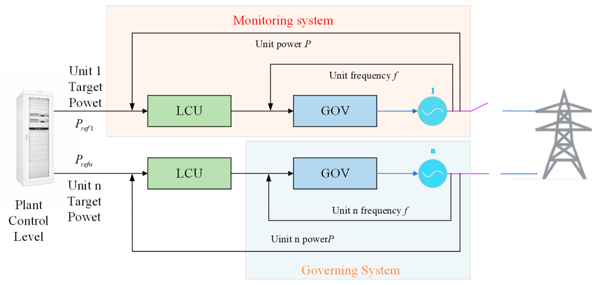
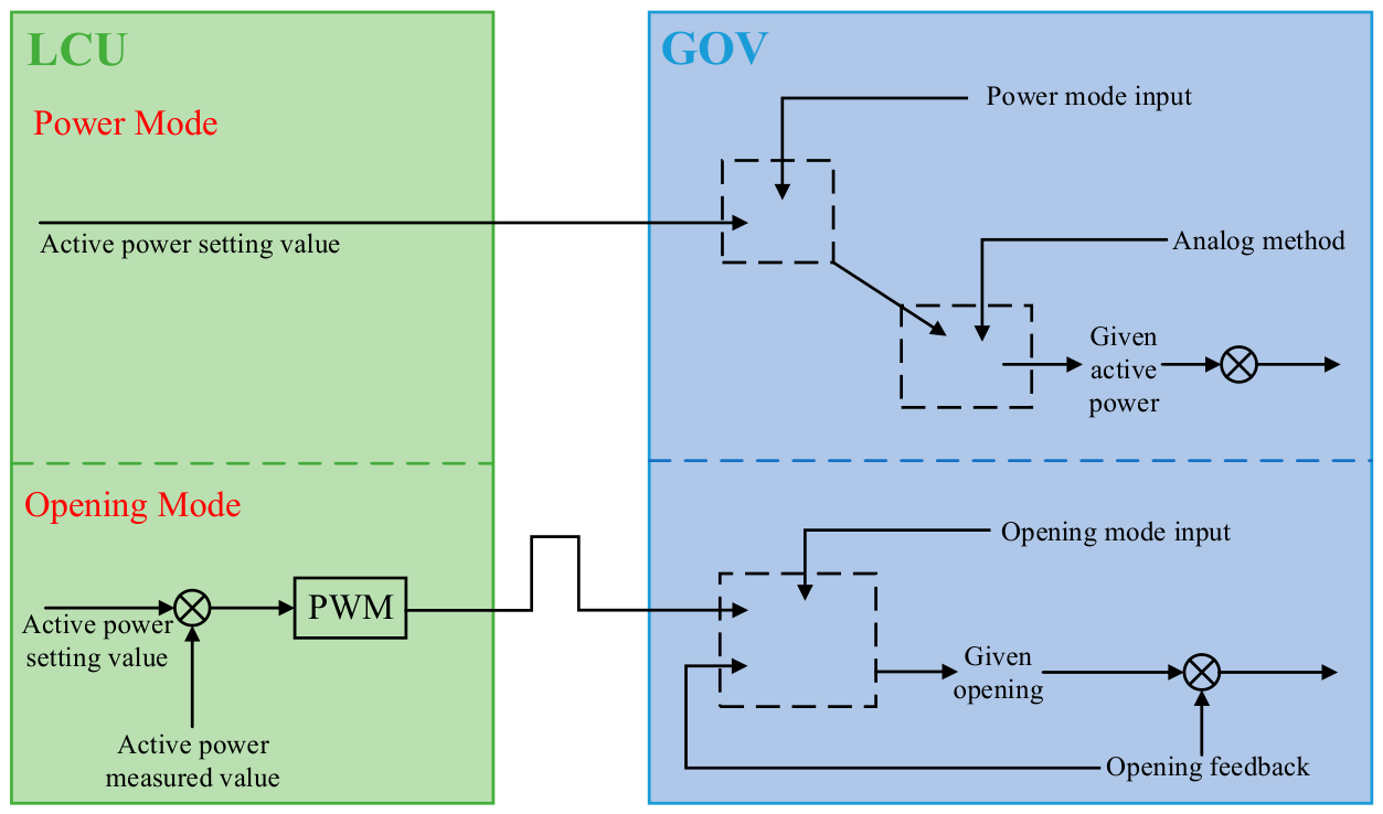
Under a hydro–wind–solar complementary operation environment, hydropower units undertake the primary regulation task, and the Automatic Generation Control (AGC) process is illustrated in Figure 1. Firstly, the overall active power command of the hydropower plant at a certain moment is transmitted to the next level, i.e., the plant control level (PCL) of the hydropower plant through the grid dispatching center, and the PCL sends the power regulation command of the whole plant unit to the local control unit (LCU) of the relevant units that undertake the regulation task in accordance with the previously established load distribution rules. The LCU uses the preset pulse width modulation (PWM) in the equipment to complete the task of correcting the active power. The specific control law is as follows: when the actual active power output of the unit and the active power command assigned by the LCU exceed the set power deadband, the difference between the two power values and the absolute value is the basis for the LCU to send power pulses, and the increase/decrease pulses are selected according to the direction of the deviation. The final criterion for the end of the process in the current regulation cycle is whether the new real-time measured power deviation is again within the power deadband. These continuous active power correction pulses from the LCU are converted by the governor into a command to correct the opening of the guide vane one at a time, and finally, the servomotor controls the guide vane in the specified direction to achieve the active power correction [21]. The focus of the article is on the red dashed box section in Figure 2, which can also be called the monitoring system power closed-loop regulation process.

The block diagram of the typical control mode of the monitoring system currently in large-scale use in the southwest China power grid is shown in Figure 1. Since the opening mode is the most basic and reliable control mode of the turbine regulation system at this stage, most of the main hydropower unit monitoring system LCU active control and speed regulation system control modes operate according to the second mode in Figure 2.

2.2. Modeling of Each Subsystem

2.2.1. Modeling of LCU Active Power Control

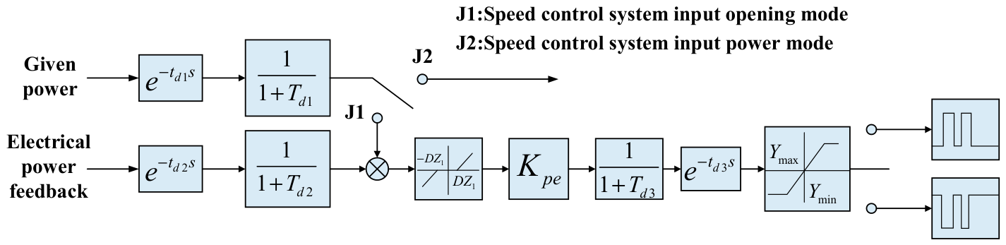
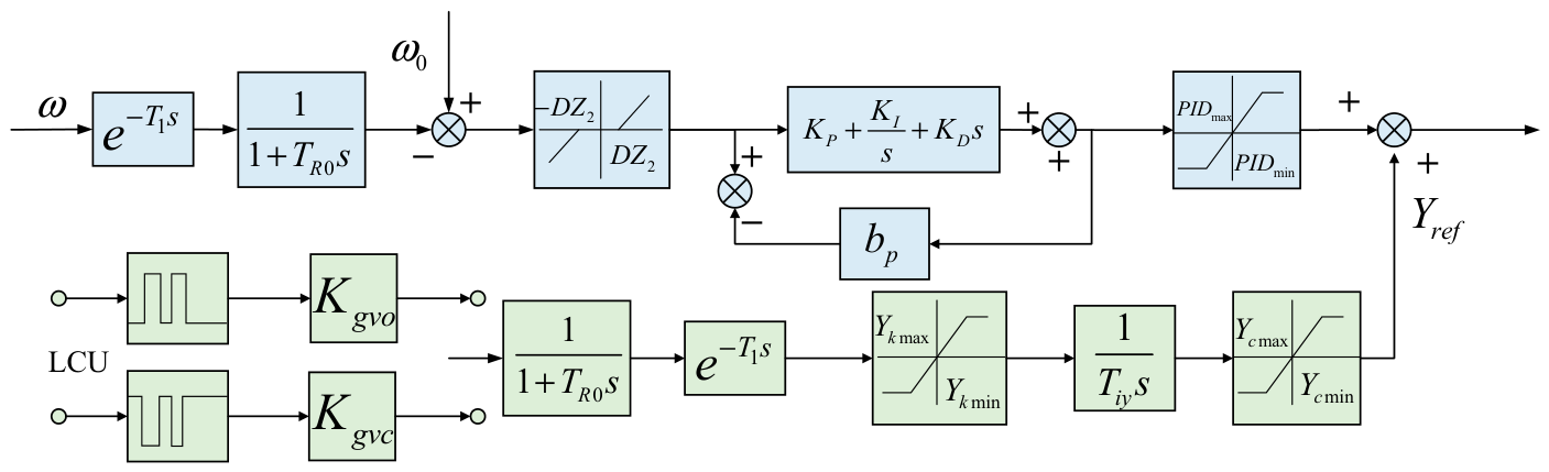
The block diagram of the LCU-based active power control system is shown in Figure 3. LCU output signal to the speed governor is a certain period of regular pulse signal, these signals cannot be directly applied to the servomotor, the speed governor needs to use the integral link of the output time accumulation characteristics, the pulse step at a time supplemented by the corresponding conversion ratio, converted into a hydropower unit guide vane opening and the formation of the opening adjustment command, compared to the commonly used electromechanical transient model of the speed governor system, the entire speed governor model adds the opening from the LCU to the final guide vane opening output, and the resulting superimposed model of the speed governor system section is shown in Figure 4.

2.2.2. Modeling of PWM

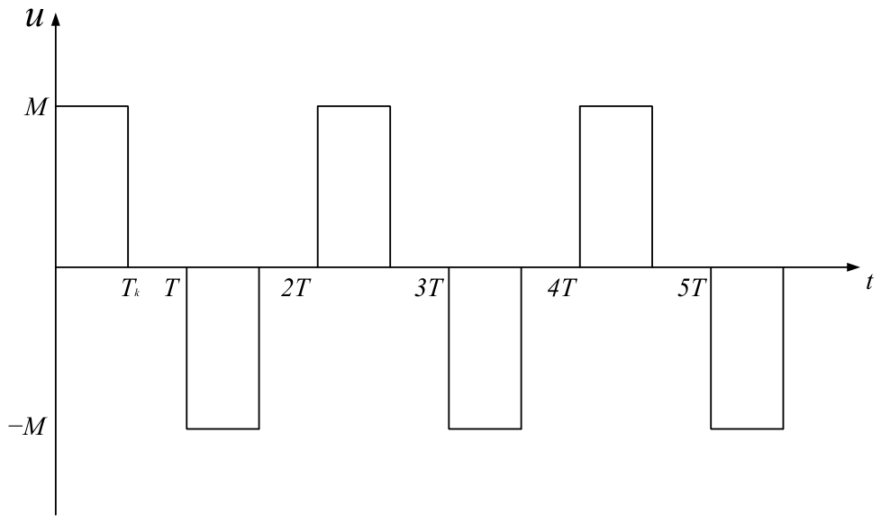
According to the previous introduction, the PWM is the most important link to achieve power adjustment, and the pulses output $u(t)$ by the PWM are calculated according to the mathematical expression of Equation (1) [10].

$$u\left(t\right)=m\left(\mathsf{\Delta }P\right)=\left\{\begin{array}{l}M\mathrm{sign}\left(\mathsf{\Delta }P\right),t\in \left[kT,kT+T_k\right]\\ 0, otherwise\end{array}\right.$$

(1)

The specific calculation of the symbolic function is shown in Equation (2).

$$sign\left(\mathsf{\Delta }P\right)=\left\{\begin{array}{l}1,\mathsf{\Delta }P>0\\ 0,\mathsf{\Delta }P=0\\ -1,\mathsf{\Delta }P<0\end{array}\right.$$

(2)

The pulse width $T_k$ is calculated as shown in Equation (3).

$$T_k=sat({\displaystyle \frac{T\left|\mathsf{\Delta }P\right|}{\beta }},0,T_{kmax})$$

(3)

2.2.3. Modeling of Water Diversion System

The modeling of the water diversion system in a hydropower unit is fundamentally based on fluid dynamics and water hammer theory. For short conduits and small transient disturbances, the rigid water hammer model can be adopted by neglecting water compressibility, pipe wall elasticity, and friction losses. Under these assumptions, the relationship between flow variation and pressure fluctuation can be described by a first-order differential equation and its corresponding transfer function, as given in Equations (4) and (5) [22,23,24].

$$\left\{\begin{array}{l}h=-T_w{\displaystyle \frac{\mathrm{d}q}{\mathrm{d}t}}\\ T_w={\displaystyle \frac{Q_0{L}_w}{g{H}_0{f}_w}}\end{array}\right.$$

(4)

$$G_w\left(s\right)={\displaystyle \frac{H\left(s\right)}{Q\left(s\right)}}=-T_{w}s$$

(5)

For long diversion pipelines, the propagation of pressure waves along the conduit cannot be neglected. Under the assumption that head loss is ignored, the elastic water hammer dynamics can be reformulated as an equivalent delay-type transfer relation:

$$G_w(s)={\displaystyle \frac{H(s)}{Q(s)}}=-2{\sigma }_w{\displaystyle \frac{1-e^{-T_{r}s}}{1+e^{-T_{r}s}}}$$

(6)

where ${\sigma }_w\stackrel{\mathsf{\Delta }}{=}{\displaystyle \frac{T_w}{T_r}}$ and $T_r\stackrel{\mathsf{\Delta }}{=}{\displaystyle \frac{2L_{wt}}{a}}$ denote the hydraulic gain coefficient and the pressure-wave travel time, respectively. Equation (6) is an equivalent reformulation of the classical elastic water-hammer transfer relation.

To facilitate controller design and system analysis, the delay term in (6) is approximated using a second-order Pade expansion. Consequently, a reduced-order rational model of the diversion system can be obtained as:

$$G_{w,p}(s)={\displaystyle \frac{H(s)}{Q_t(s)}}=-{\sigma }_w{\displaystyle \frac{T_{r}s}{1+\frac{T_r^2{s}^2}{12}}}$$

(7)

This approximation is valid for small-signal analysis and low-frequency operating conditions.

2.2.4. Modeling of Speed Governor

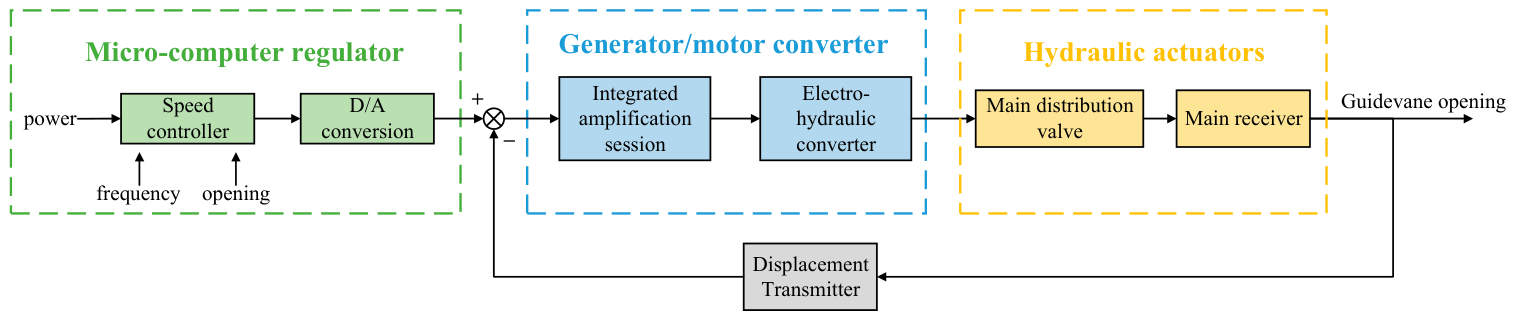
This subsection mainly discusses the mathematical model of microcomputer type speed governor, which is widely used in engineering. The hydro turbine speed governor is the core equipment of the hydro turbine regulation system, which is mainly composed of two parts: a microcomputer regulator and a hydraulic actuator. Moreover, its basic structure block diagram is shown in Figure 5.

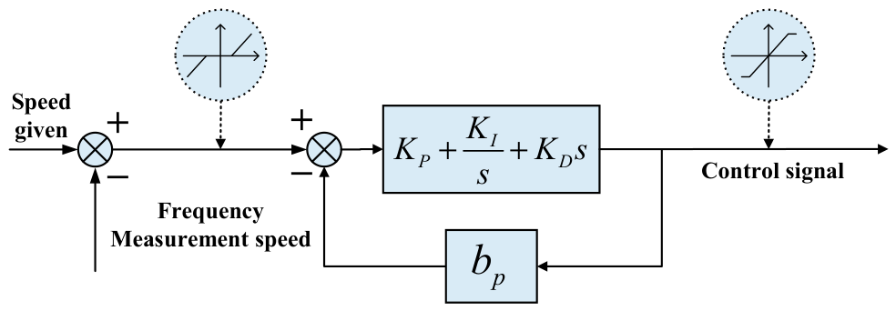
The microcomputer regulators of hydro turbines put into use or to be put into use in China have all adopted the PID control strategy, and the parallel-type PID control law is one of the most widely favored strategies; its structure block diagram is shown in Figure 6. The block diagram of the speed governor shown in Figure 6 is translated into the corresponding transfer function, as shown in Equation (8).

$$\left\{\begin{array}{l}{G}_c(s)=K_P+{\displaystyle \frac{K_I}{s}}+K_{D}s\\ G_{PID}(s)={\displaystyle \frac{u(s)}{x_c(s)-x(s)}}={\displaystyle \frac{G_c(s)}{1+b_p{G}_c(s)}}\end{array}\right.$$

(8)

In practical engineering applications, the PI regulation law is generally used after grid-connected operation of the hydro turbine, at which time the corresponding differential equation and transfer function of the regulator are simplified as shown in Equation (9), respectively [25].

$$G_{PI}(s)={\displaystyle \frac{K_{P}s+K_I}{(1+b_p{K}_P)s+b_p{K}_I}}$$

(9)

After receiving the weak electrical control signal from the microcomputer regulator, the weak electrical control signal is converted to the mechanical hydraulic model applicable to the hydraulic actuator through the integrated amplification and power-hydraulic signal conversion link, and then through the control of the corresponding equipment for action, such as the auxiliary catcher, the main pressure distribution valve, the main servomotor, etc., and finally to achieve the purpose of controlling the degree of opening and closing of the hydraulic turbine guide vane. The hydraulic actuator, after ignoring the reaction time constant of the auxiliary servomotor, can be written in the form of a differential equation shown in (10) with the transfer function of (11).

$$T_y{\displaystyle \frac{dy}{dt}}+y=K_{0}u$$

(10)

$$G_{servo}\left(s\right)={\displaystyle \frac{K_0}{T_{y}s+1}}$$

(11)

2.2.5. Modeling of Hydro-Turbine

In principle, the dynamic characteristics of the turbine need to be used in the analysis of the transition process, but the accurate method to obtain the dynamic characteristics of the turbine is still a difficult breakthrough problem in engineering. Therefore, for the case when the rate of change in hydraulic turbine operating conditions is low and the speed does not change beyond a certain value ($\omega <1 {\mathrm{s}}^{-1}$), its static characteristics can be used instead of dynamic characteristics for modeling and analysis; the specific relationship between the parameters is shown in Equation (12).

$$\left\{\begin{array}{l}{M}_t=M_t(Y,n,H)\\ Q_t=Q_t(Y,n,H)\end{array}\right.$$

(12)

This simplification is intended for conventional AGC operating conditions with relatively small operating-point variations and limited speed deviation, under which the static characteristic model can still capture the main input–output relationship of the local power closed-loop regulation process. However, for faster AGC actions, larger power-step commands, or stronger hydraulic transients, neglecting the turbine dynamic characteristics may underestimate transient lag, overshoot, and hydraulic coupling effects. As a result, the absolute values of regulation time, ITAE, and even the exact location of the optimal parameter set may be affected. Therefore, the present model is mainly used to reveal the parameter-influence mechanism and to support comparative optimization under conventional AGC conditions rather than to provide a high-fidelity prediction for all fast transient scenarios.

By linearizing Equation (12) around the operating point and neglecting higher-order terms, the six-parameter linear model of the hydro turbine can be derived by omitting the second-order and higher-order terms when considering a small range of variation in the parameters, as shown in Equation (13), where the parameters are expressed in the form of relative values of deviations [26].

$$\left\{\begin{array}{l}{m}_t=e_{y}y+e_x{x}_t+e_{h}h\\ q_t=e_{qy}y+e_{qx}{x}_t+e_{qh}h\end{array}\right.$$

(13)

where $e_h=\partial m_t/\partial h$, $e_x=\partial m_t/\partial x$, $e_y=\partial m_t/\partial y$, $e_{qh}=\partial q_t/\partial h$, $e_{qx}=\partial q_t/\partial x$, $e_{qy}=\partial q_t/\partial y$.

3. Quantification of Wear on Hydropower Unit Servomotor

Even if generation control rate and range are not as limited as before and units could respond much faster, it may still be undesirable to maneuver generation in an attempt to match fast-varying components of the market demand. Such operations would increase wear and tear on speed governing equipment such as hydro-turbine units [27]. Quantifying the influence of the main parameters on the equipment wear in this process can help us to optimize the parameters in the future.

3.1. Visualization of Control Parameters Affecting Servomotor Wear

The AGC function of the hydropower unit requires the monitoring system to give the power command, and the speed governor to implement the command execution. This power closed-loop correction process involves more links, and the core link of the regulation process is PWM. The schematic diagram of the PWM output is shown in Figure 7.

The key control parameters affecting the PWM output pulse characteristics are $T$, $\beta$, $T_{kmax}$, $T_{kmin}$ and $T_{iy}$. In the hydropower unit speed governor, the control function is mainly realized by the actuator of the signal, i.e., the servomotor. Analyzing the action law of these main control parameters in the transition process of active power regulation and the influence of some parameters on the working intensity of the servomotor can help us to further deepen our understanding of the AGC characteristics of hydropower units.

Previous studies have quantified the equipment wear by measuring the number of movements, movement distance, and movement direction of the equipment using sensors [20]. Among these indicators, movement distance has a clear tribological implication because larger cumulative relative displacement in the servomotor-related moving pairs generally leads to higher frictional work and stronger cumulative surface interaction. In addition, frequent start-stop actions and reversals may intensify boundary-friction effects and local mechanical impact, which are also unfavorable to long-term equipment health. However, there are always measurement errors for smaller movements. In contrast, this paper quantifies the influence of these parameters on the wear through wear-related proxy indicators that characterize the actuation intensity of the device. Since the conversion relationship between the width of the pulse and the action amplitude of the subsequent actuator is fixed, the PWM pulse signal in the LCU–governor–servomotor execution chain can be regarded as an electrical representation of the subsequent mechanical actuation process. Specifically, pulse width corresponds to the amplitude of a single guide-vane opening adjustment, while the cumulative pulse width reflects the variation trend of cumulative action distance; meanwhile, pulse number reflects the actuation frequency of the servomotor. Therefore, this paper considers the influence of the calculation parameters on the number of pulses as well as the sum of pulse widths, which are two key indicators, to indirectly evaluate the wear-related actuation burden of the servomotor, rather than relying solely on the direct measurement of small mechanical displacements. Two testing methods, a power sine input signal and a power step signal, are used to visualize the parameter influence on the wear of the servomotor. The power sine input signal amplitude is 0.05 pu, and the oscillation frequency is 0.04 Hz; the power step is set as the transition process of active power increasing by 10% of the rated value, and both simulation durations are set to 100 s. The influence of the parameters is analyzed by recording the change process of increasing pulse width, decreasing pulse width and the number of pulses during the adjustment of the unit when the parameters are modified. It should be noted that the proposed pulse-based indices are wear-related proxy indicators rather than direct measurements of mechanical degradation. Nevertheless, they provide a practical and physically interpretable basis for comparing different PWM parameter settings from the perspective of servomotor wear tendency.

3.2. Quantitative Analysis of Control Parameters Affecting Servomotor Wear

(1)

Modifying the pulse period T:

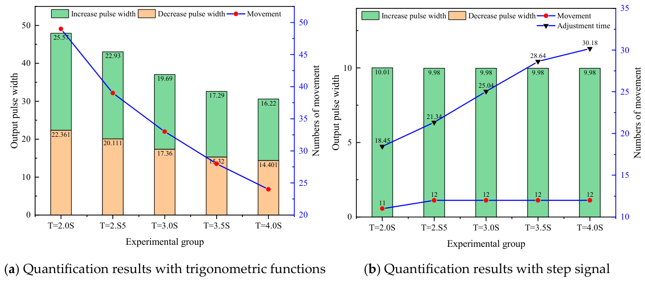
When using the trigonometric function for the test, it can be seen from Figure 8a that the number of pulses decreases almost linearly as the set value of the pulse period $T$ gradually increases, from 49 pulses at $T=2.0 \mathrm{s}$ to 24 pulses at $T=4.0 \mathrm{s}$. Both the increasing and decreasing pulse widths decrease accordingly, but the trend is slower compared to the number of pulses. When the power step signal is used for the test, the change in the setting value of $T$ hardly affects the number of pulses and pulse width, and the impact on the power transition process is mainly reflected in the regulation time. Since the maximum pulse duration limit is unchanged, the pulse width is the same in each regulation cycle at the beginning of regulation, i.e., the amplitude of the guidevane action is the same in each regulation cycle, but the larger the regulation cycle, the longer the time that the guidevane opening does not change in each cycle, which eventually leads to the increase in the whole active power regulation process time, which is eventually reflected in the regulation time, from 18.45 s at $T=2.0 \mathrm{s}$ to 30.18 s at $T=4.0 \mathrm{s}$.

(2)

Pulse duration calculation scale factor $\beta$:

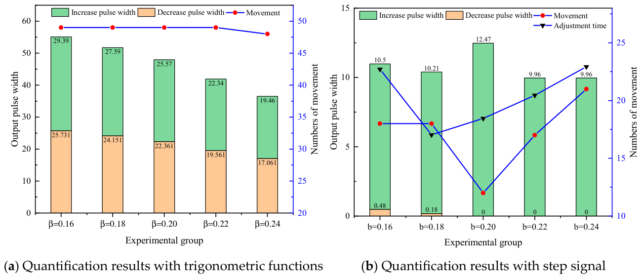
When using the trigonometric function to do the test, the number of pulses under different pulse duration calculation scale factor $\beta$ is almost the same, and only the pulse width decreases gradually with the increase in the set value, which is similar to the effect of modifying the pulse period, and the characteristics that the width of increasing pulses is greater than the width of decreasing pulses are also more consistent. Some indicators of the regulation process are shown in Figure 9b. At the beginning of the regulation process, the regulation process under different $\beta$ is almost the same, and the period when $\beta$ it mainly takes effect is the second half of the power correction process, i.e., the stage when the distance from the target value is closer. As $\beta$ increases from 0.16 to 0.24, the adjustment time decreases from 22.72 s to 17.04 s and then increases to 22.93 s.

From the above analysis, the role played by $\beta$ in the regulation process is mainly to amplify the difference between the actual value of active power and the target value. Therefore, in the case of the same other parameters, the smaller the $\beta$, the larger the difference after amplification, but in the regulation period at the beginning of the regulation, the pulse duration is generated in accordance with the maximum pulse duration limit, so the initial active power regulation process is under different $\beta$ and the waveform is almost the same. However, when approaching the target value, a smaller set value of the power regulation process at this time, the power difference is greater in comparison, which will lead to more regulation cycles.

(3)

Maximum pulse duration limit $T_{kmax}$

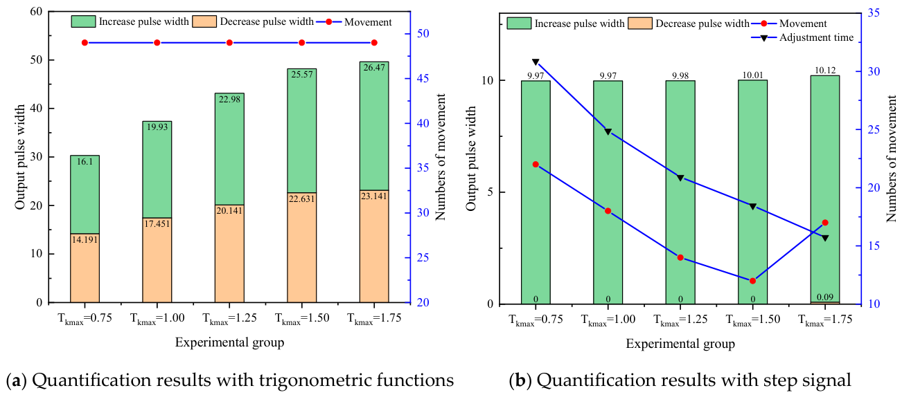
When using the trigonometric function to do the test, as the setting value of $T_{kmax}$ gradually increases, the number of pulses is not affected, are maintained at an identical level. And the incremental pulse width and the decremental pulse width both increase accordingly, resulting in the final total pulse width getting larger and larger, but the change in this pulse width is not linear, the increase in pulse width will slowly decrease with the gradual increase in the setting value in the cycle, when the maximum pulse duration limit is the same as the pulse period, the total pulse width will also come to the maximum value, and the difference between the incremental and decremental pulse width will also get larger and larger with the increase in the parameter setting value.

Some indicators of the adjustment process are shown in Figure 10b. In the case of the same set target value, with the gradual increase in the set value of $T_{k\max }$, the action amount of the guidevane opening during the pulse generation cycle gradually increases, and the adjustment time consumed by the power correction process becomes shorter and shorter, from 42.88 s at $T_{kmax}=0.5$ to 14.56 s at $T_{kmax}=2.0$, reducing the adjustment time by 66%. The gradual increase in the setting value of $T_{kmax}$ accelerates the adjustment speed of the whole power adjustment process. Meanwhile, observing the pulse indicators for $T_{kmax}=0.75$ as well as for $T_{kmax}=1.5$, it can be found that the former outputs almost twice as many pulses as the latter in order to achieve the same regulated target value of active power. Each pulse means a change in the opening of the guidevane, which means a complete action of the hydraulic equipment controlling the action of the guidevane. And in $T_{kmax}=0.75$, when approaching the regulation target value, there are more pulses with very small pulse width, which eventually leads to the whole process of the guidevane action occurring more times, which will greatly increase the work intensity of the equipment, have a greater impact on the life of the equipment, but also will not be conducive to the long-term safe and stable operation of hydropower plant equipment.

(4)

Minimum pulse duration limit $T_{kmin}$

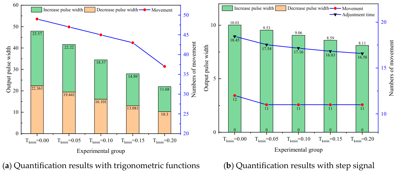
From Figure 11a, as the setting value of $T_{kmin}$ gradually increases, the change trend of the incremental pulse width and the decremental pulse width is opposite to the maximum pulse duration limit. The difference between the incremental and decremental pulses, the total pulse width, and the incremental and decremental pulse widths becomes smaller and smaller as the parameter increases. The number of pulses is no exception, gradually decreasing from 49 at $T_{kmin}=0.00$ to 37 at $T_{kmin}=0.20$, and the total pulse width also decreases from 47.931 s to 21.98 s, a decrease of more than 50%.

As can be seen from Figure 11b, with the gradual increase of $T_{kmin}$, there is a large difference in the steady-state value reached at the end of the final regulation process, and the deviation of the steady-state value after the completion of the regulation process from the set power target value becomes larger and larger, even when $T_{kmin}=0.20$, there is an error of up to 0.94% between the two. However, when modifying $T_{kmin}$, the regulation times all vary within a very small range of 17 s to 18.5 s, which shows that the $T_{kmin}$ action does not include modifying the rate of the regulation process. Although the number of pulses and the total pulse width are decreasing due to the gradual increase in the parameter settings, this is at the expense of the regulation accuracy.

(5)

Opening integral conversion parameters $T_{iy}$

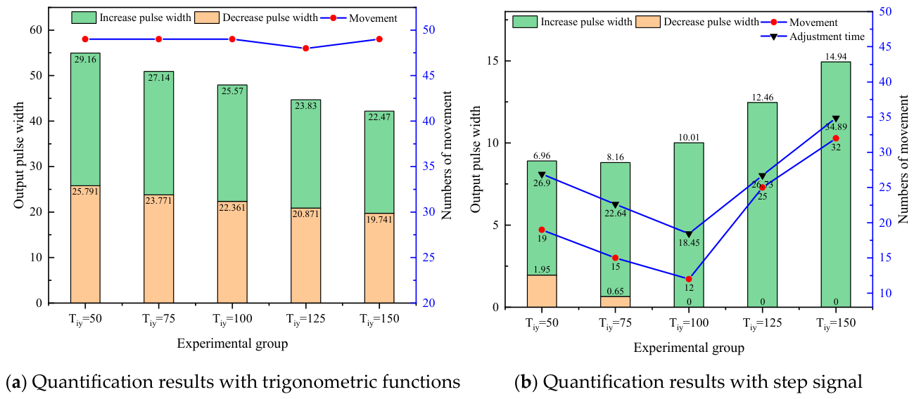
As can be seen from Figure 12a, the modification of $T_{iy}$ has almost no effect on the number of pulses, and the effect of $\beta$ is almost similar, and the gap between increasing and decreasing pulse widths becomes smaller and smaller as $T_{iy}$ gradually increases, and some indicators of the regulation process are shown in Figure 12b. From the results, $T_{iy}$ mainly affects the action speed of the guide lobe in the power regulation process. The larger $T_{iy}$ is, the slower the action rate of the guidevane is, and the slower the rate of active power regulation of the unit is, but it is not a monotonically increasing trend reflected in the regulation time. This is because when $T_{iy}$ is small, such as when $T_{iy}=50$ and $T_{iy}=75$, the whole regulation process has a large backward adjustment and overshoot, even leading to the phenomenon of power oscillation up and down in the regulation process, which also makes the whole regulation process longer and finally reflected in a longer regulation time.

4. Multi-Objective Optimization Framework for AGC Parameters

4.1. Description of the Problem

The results of the research on PWM parameters can be found that in the process of active power regulation, these parameters have a greater impact on the number of speed governor actions and action amplitude, and unreasonable parameter settings will increase the work intensity of the equipment and have a greater impact on the life of the equipment. The previous chapter quantified the impact of control parameters on equipment wear by using reasonable quantification methods, based on which we hope to help the hydropower units, combined with the regulation requirements, in a reasonable range of these parameters, preferably, to achieve a reasonable planning of the use of plant equipment to ensure efficient and long-term stable operation of the equipment.

4.2. Optimization Model

Combined with the operating characteristics of hydropower units, the optimization objective considering the response rate and regulation accuracy in the transition process of AGC power regulation is constructed, and a multi-objective optimization model of the transition process is established. The model can comprehensively consider multiple constraints, such as the regulation guarantee requirements of each hydropower unit and the mechanical performance of the speed governor, and optimize the PWM control parameters through an intelligent optimization algorithm to optimize the unit regulation time, steady-state difference, and key indexes of the ITAE transition process in the power regulation transition process.

4.2.1. Objective Functions

In the AGC power regulation transition process, its rapidity and smoothness are a pair of opposing performance indicators, where the response rate is often quantified by the power transition process regulation time, and the smoothness is quantified by the unit power ITAE, which is a highly comprehensive indicator. In this paper, the objective function is shown in Equations (14) and (15), considering the fast and smooth characteristics of the power transition process, with the unit regulation time and the unit power ITAE as the optimization objectives.

(1)

Objective function 1

$$\min F_{obj-1}\prime =t_s$$

(14)

(2)

Objective function 2

$$\min F_{obj-2}={\displaystyle {\displaystyle \underset{0}{\overset{t}{\int }}}t\left|e\left(t\right)\right|dt}$$

(15)

4.2.2. Constraints

In order to ensure transmission quality, the grid will generally have the following requirements for AGC of hydropower units.

(a)

Response rate requirement: the average load regulation per minute (i.e., load regulation rate) during AGC load regulation should be not less than 50% of the rated load.

(b)

Regulation accuracy requirement: after the execution of the AGC command of the hydropower unit, the error between the actual output of the whole plant and the target value of the whole plant, and the percentage of the capacity of the starting unit, should not be greater than 3%. The percentage of error between the actual output of the whole plant and the target value of the whole plant and the capacity of the starting unit during the execution of the dynamic process of AGC command of the hydropower unit shall not be greater than 5%.

(c)

Equipment action accuracy requirements: when the power is given or the opening degree is given as constant, the deviation of the actual active power or opening degree of the unit from the given value should be −1%~+1%.

(d)

Parameter setting constraints: the maximum pulse duration limit shall not exceed the pulse period, i.e., $T_{kmin}\le T_{kmax}$; the minimum pulse duration limit shall not exceed the maximum pulse duration limit, i.e., $T_{kmax}\le T$.

4.3. Multi-Objective Optimization Algorithm

NSGA-II is a widely used multi-objective optimization algorithm [28,29], which has good results in quickly finding Pareto fronts and maintaining population diversity, and is also suitable for solving multi-objective optimization models in AGC power regulation transition processes.

4.4. Multi-Objective Optimization Process for Control Parameters

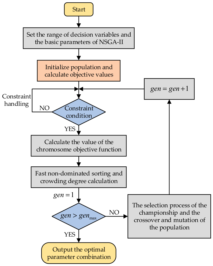
The multi-objective optimization model solving process for AGC parameters based on the NSGA-II algorithm in this section is shown in Figure 13, and the specific steps are as follows.

Step 1: Set the range of values of multi-objective optimization parameters $\left[\beta T_k T_{kmax} T_{kmin} T_{iy}\right]$ for AGC. Initialize some basic parameters of the NSGA-II algorithm, e.g., set the number of iterations of the algorithm $gen=50$.

Step 2: Initialize the population with random values in the specified range of decision variables according to $P=P_{min}+rand\left(0,1\right)\ast \left(P_{max}-P_{min}\right)$ and calculate the objective function values corresponding to chromosomes within the population.

Step 3: Extract the matrix of decision variables on all chromosomes, i.e., the AGC parameters, substitute them into the simulation model established in the article, solve the closed-loop power regulation transition process, and calculate the characteristic parameters and objective functions F1 and F2; then, post-constraint processing is performed for the individuals that violate the constraints (a) to (d) in Section 4.2.2.

Step 4: Perform fast non-dominated sorting and crowding degree calculation for all chromosome variables within the population, initialize $gen=1$; if at this point $gen>ge{n}_{max}$, output all chromosome variables of the population as the optimization frontier, and select the optimal result according to the servomotor wear at the frontier; otherwise, proceed to step 5.

Step 5: Tournament selection process and population crossover variation:

(1)

Randomly select two individuals, giving preference to the individual with a high-ranking order, and if the ranking order is the same, preferably select the individual with a high degree of crowding to enter the tournament.

(2)

Cross-mutation to generate offspring individuals based on the tournament-selected parent, suitable for reproduction.

(3)

Generating a new population by putting the two generations of offspring and parent populations together for non-dominance sorting;

Step 6: $gen=gen+1$; return to Step 3.

5. Case Study

Based on the numerical simulation model of AGC of the hydropower unit established in Section 2 above, the effectiveness of the AGC parameter optimization strategy based on NSGA-II proposed in Chapter 4 of this paper is verified.

5.1. Simulation Model

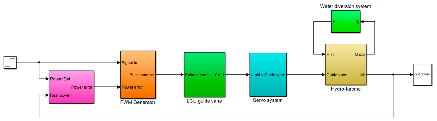
The overall mathematical model of the AGC process of hydropower units can be obtained by integrating the mathematical models of all subsystems involved in the AGC function described in Chapter 2 and connecting the input and output links appropriately. The overall mathematical model was solidified in the MATLAB/Simulink R2023b platform in a modular way, and the established visualized numerical simulation model of AGC of a hydropower unit is shown in Figure 14.

5.2. Optimize Initial Conditions and Parameter Settings

After completing the establishment and initialization of the simulation model of the AGC function of the hydropower unit, the optimization of the parameters of the closed-loop power adjustment process can be started, at which time the parameters of the optimization algorithm and the basic parameters of the simulation model operation need to be set, respectively, as follows.

(1)

The parameters of the NSGA-II algorithm are maximum number of iterations $gen=100$, chromosome population size $pop=300$, mating pool size $pool=150$, number of tournament participants $tour=2$, number of objective functions $M=2$, dimension of decision variables $V=5$, distribution index of crossover and mutation algorithm $mu=20$, crossover probability and mutation probability $crossover=0.9$. In addition, the upper and the lower limits of the decision variables are $\max \_range=[0.4,3.0,1.0,0.1,150]$ and $\min \_range=[0.1,1.5,0.0,0.0,50]$.

(2)

The parameters of the simulation model for the AGC function of hydropower units are: the simulation duration of the closed-loop power adjustment transition process $T_{sim}=100 \mathrm{s}$, the numerical simulation time step $\mathsf{\Delta }t=0.01 \mathrm{s}$.

(3)

Other parameters used in the simulation model are shown in

Table 1. Simulation model parameters.

Parameters	Value	Parameters	Value	Parameters	Value	Parameters	Value
$K_P$	1	$T_y$	0.2	$e_x$	−1	$e_{qh}$	0.5
$K_I$	6	$T_w$	2.738	$e_y$	1	$T$	2
$K_D$	0	$T_a$	9.11	$e_h$	1.5	$T_{kmax}$	1.5
$e_p$	0.04	$T_{iy}$	100	$e_{qx}$	0	$T_{kmin}$	0
$D{Z}_1$	0.001	$K_{pe}$	4.2	$e_{qy}$	1	$\beta$	0.2

.

5.3. Optimization Results and Comparative Analysis

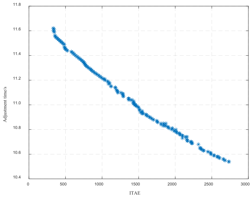
Based on the simulation model, the operating parameters and the initial conditions of the optimization algorithm are set, and the multi-objective optimization of PWM control parameters is carried out according to the solving strategy of the simulation model of the AGC function of hydropower units. After the optimization results are obtained, some representative results of the optimization frontier are selected and compared with the optimization results and the measured results to verify the effectiveness of the optimization strategy. The optimization results of the NSGA-II algorithm are plotted on the target plane of the adjustment time and ITAE, and the obtained results are shown in Figure 15.

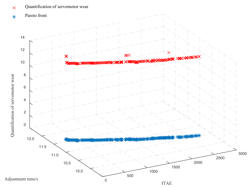
From the optimization frontier results in Figure 15, the optimization results are more uniformly distributed in the target plane, with the distribution range of objective function one ranging between a small range of 10.5 s to 11.7 s, and the distribution range of objective function two ranging from 300 to 2800, spanning a large range. From the aforementioned optimization process, it can be seen that the optimization frontier should be output at this time for all chromosomes of the population, and the power closed-loop transition process should be calculated according to the decision variables of each chromosome to obtain the corresponding quantified value of the servomotor wear $F_3=\mathrm{Movement}+\mathrm{Distance}$ for each chromosome, and the chromosome with the smallest quantified wear value should be selected as the optimal result. The optimized results corresponding to all chromosomes of the population and the results of the wear quantization values are plotted in the three-dimensional plane, and the obtained results are shown in Figure 16.

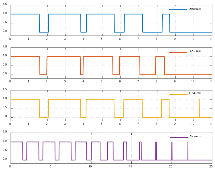
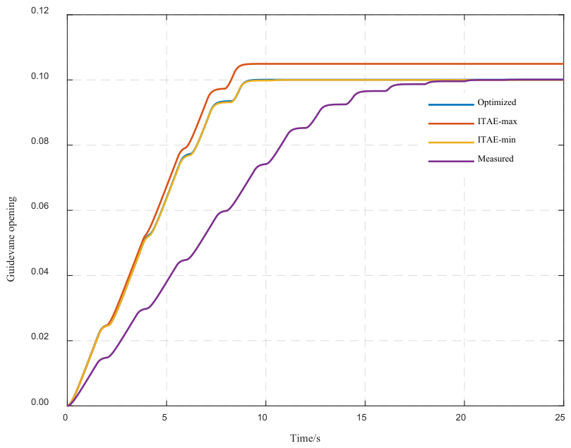
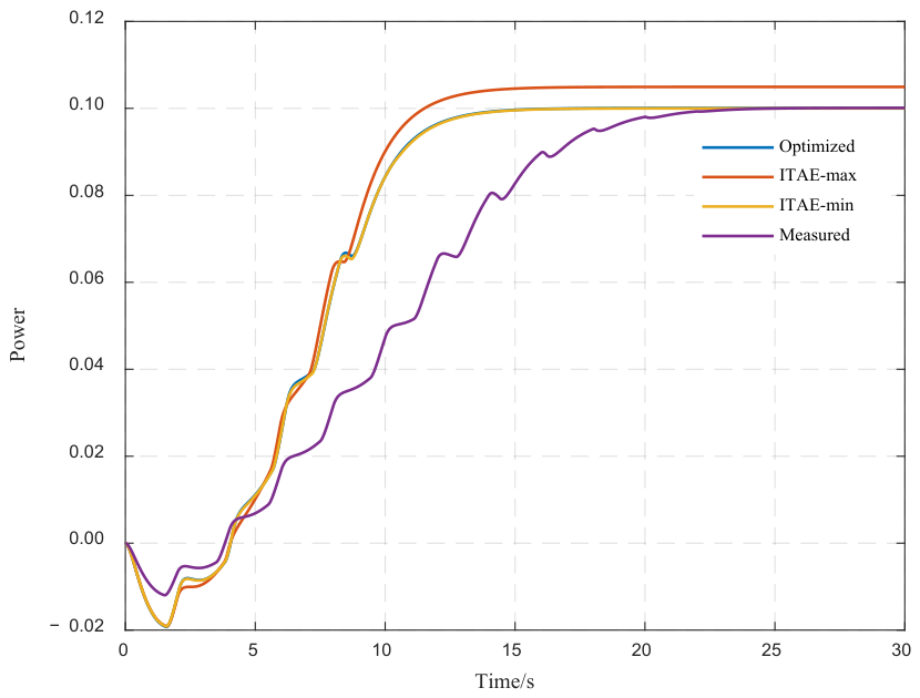
From the results in Figure 16, the distribution of the wear quantization values of the chromosomes is very concentrated, between 11.2 and 12, and only individual chromosomes have quantified wear values greater than 12. The smallest of these is 11.26, and this chromosome is the optimized result currently. The optimized results are compared with the maximum ITAE, minimum ITAE and measured PWM parameters in the frontier, and the closed-loop power regulation transition process is simulated to calculate the key parameters of the transition process in order to obtain a more intuitive comparison. The dynamic indexes of the closed-loop power regulation transition process of the selected chromosome are shown in

Table 2. Dynamic indexes of power adjustment transition process for different cases.

Case	Quantified Values of Servomotor Wear	Adjustment Time	Stable Value	ITAE
Optimized	11.26	11.55	0.1001	365
ITAE-max	11.64	10.54	0.1049	2734
ITAE-min	12.30	11.62	0.1000	334
Measured	10.01	18.40	0.1001	720

. The corresponding pulse output, guidevane opening and power dynamic process are shown in Figure 17, Figure 18 and Figure 19.

From the dynamic indicators in Table 2 and the dynamic processes in Figure 17, Figure 18 and Figure 19, the actual situation of the power closed-loop rate regulation transition process has a regulation time of 18.40 s, which has exceeded the requirement for the response rate limit, i.e., the average load regulation per minute in the AGC load regulation process should be no less than 50% of the rated load. Although the performance on the quantified value of the servomotor wear is even better than the result on the frontier, which is the minimum 10.01, the performance on the action intensity (total action amplitude divided by the number of actions) is poor, as shown by the more frequent pulses with very small pulse widths, these frequent small displacement actions will undoubtedly increase the wear of equipment and reduce the life of the equipment [20].

It should be noted that although the differences in steady-state values among the cases in Table 2 are numerically very small, such differences have limited practical engineering significance within the allowable regulation accuracy range. In practical AGC operation, steady-state deviations within ±1% are generally considered acceptable and have a negligible impact on system performance. Therefore, compared with steady-state differences, dynamic performance indicators such as adjustment time and servomotor wear are more critical for evaluating the effectiveness of parameter optimization. It also confirms the necessity of the study on one side.

The optimized fronts all meet the requirements in terms of response rate, and the selected chromosome with the maximum value of ITAE has a better performance in terms of regulation time; however, it does sacrifice the steady-state value as the price, and there is a steady-state error close to 5%, although the single unit still meets the regulation requirements, but it is not conducive to the regulation of the whole plant. The magnitude of the steady-state difference can also reflect the accuracy of the ITAE calculation results to a certain extent. Similarly, for the chromosome with the minimum value of ITAE selected, the steady-state difference value is rightfully the best performance among the four groups of results, but the quantized value of the servomotor wear is the maximum among the four groups of results, which can also be explained from the perspective of regulation accuracy, to get higher regulation accuracy, there will inevitably be different degrees of fine-tuning to ensure the minimum steady-state difference value, which eventually leads to a larger quantized value.

The optimized chromosome from the frontier has a more balanced performance in various dynamic indicators of the power closed-loop transition process, and the overall transition process is very similar to that of the ITAE minimum chromosome, but the biggest difference is the lack of the last very small pulse width pulse emission, and the difference in steady-state difference is only 0.01% compared to the best-performing ITAE minimum chromosome, but in the adjustment time and the quantized value of the catcher both perform much better. It can be said that the optimized result is the most balanced set of parameters in terms of comprehensive performance, and it also proves the rationality and scientific of the multi-objective optimization framework of AGC parameters proposed in this paper.

6. Conclusions and Discussion

In the study of this paper, the influence of parameters on the wear of the servomotor of the hydropower unit during AGC is clarified and reasonably quantified, and a multi-objective optimization framework for AGC parameters is established. By establishing a mathematical model reflecting the operating mechanism and characteristics of the AGC of hydropower units, focusing on the influence and mechanism of action of the main parameters on equipment wear, and finally establishing a framework for parameter optimization, the main findings and conclusions obtained in the paper are summarized as follows.

• The key control parameters of the PWM do have a large impact on the working intensity of the equipment, and the number of pulses and pulse width can be used to quantify the impact of these parameters on the wear of the servomotor more reasonably.
• Among the key control parameters of the PWM: the pulse period mainly affects the interval time of the equipment action; a smaller pulse duration calculation scale factor will lead to more adjustment cycles, so that the equipment appears to be adjusted in different action directions; the maximum and minimum pulse duration limits have the greatest impact on the working intensity of the equipment, the maximum pulse duration limit will significantly affect the action range of the equipment, while the minimum pulse duration limit affects the action distance of the device by affecting the adjustment accuracy; the opening integral conversion parameter affects the adjustment rate, and the smaller parameter significantly increases the wear of the device.
• The multi-objective optimization framework of AGC parameters proposed in this paper is both rational and scientific, and the results selected from the frontier using quantified values of device wear are more balanced in various dynamic indicators of the power closed-loop transition process, which can effectively improve the quality of the transition process.

The results obtained in this study should be interpreted within the scope of the adopted modeling assumptions. In the present work, the hydro–wind–solar complementary operation is treated as the engineering background motivating frequent AGC actions, while the actual modeling scope is restricted to the unit-level AGC execution chain of the hydropower unit. Accordingly, wind and photovoltaic fluctuations are equivalently represented as variations in the active power reference, rather than being modeled through detailed renewable-generation dynamics. In addition, the hydro-turbine model is linearized around the operating point, and static turbine characteristics are used under small operating-condition variations. Therefore, the proposed framework is more suitable for analyzing parameter effects and optimization trends under conventional AGC scenarios and small-to-moderate disturbances, whereas its quantitative accuracy under faster AGC actions, stronger nonlinear hydraulic transients, or more complex source-grid interactions should be further verified using higher-fidelity models.

Another point that should be emphasized is the physical meaning and boundary of the wear-related indicators used in this paper. The proposed pulse-based indices are not intended to be direct measurements of mechanical degradation; rather, they are wear-related proxy indicators for the actuation burden of the servomotor. Their rationale is that, in the LCU–PWM–governor–servomotor execution chain, pulse width is converted into guide-vane opening motion through a fixed actuation relationship, so the cumulative pulse width reflects the variation trend of cumulative movement distance, while pulse number reflects actuation frequency. Since cumulative movement distance and frequent start-stop/reversal actions are closely related to frictional work accumulation and tribological wear tendency, these indices provide a practical and physically interpretable basis for comparing PWM parameter settings from the perspective of equipment lifetime. Nevertheless, a more explicit experimental mapping between pulse characteristics and actual mechanical degradation still requires long-term field data or dedicated test-bench validation.

From the optimization perspective, the present study adopts a two-stage strategy, in which regulation time and ITAE are first optimized to obtain the Pareto solution set, and the wear-related quantified index is then used for engineering-oriented selection within the frontier. This treatment was adopted because the wear-related index defined in this paper is derived from pulse number and pulse width, which may be coupled with dynamic-performance indices rather than forming a completely independent and strictly conflicting objective dimension. In this sense, directly formulating the wear-related index as an additional joint optimization objective is a worthwhile extension for future work, but it should be regarded as a supplement to the present framework rather than a prerequisite for its validity. Further work may also include comparisons with other multi-objective optimization algorithms, such as PSO-based or decomposition-based methods, and validation under broader operating conditions and field data.

References

1. International Energy Agency (IEA). Electricity 2026; IEA: Paris, France, 2026. [Google Scholar]
2. Renewable energy policy network for the 21st century (REN21). Renewables 2022 Global Status Report; REN21 Secretariat: Paris, France, 2022. [Google Scholar]
3. Kusic, G.L.; Sutterfield, J.A.; Caprez, A.R.; Haneline, J.L.; Bergman, B.R. Automatic generation control for hydro systems. IEEE Trans. Energy Convers. 1988, 3, 33–39. [Google Scholar] [CrossRef]
4. Daraz, A.; Malik, S.A.; Haq, I.U.; Khan, K.B.; Laghari, G.F.; Zafar, F. Modified PID controller for automatic generation control of multi-source interconnected power system using fitness dependent optimizer algorithm. PLoS ONE 2020, 15, e242428. [Google Scholar] [CrossRef] [PubMed]
5. Weldcherkos, T.; Salau, A.O.; Ashagrie, A. Modeling and design of an automatic generation control for hydropower plants using neuro-fuzzy controller. Energy Rep. 2021, 7, 6626–6637. [Google Scholar] [CrossRef]
6. Hakimuddin, N.; Nasiruddin, I.; Bhatti, T.S.; Arya, Y. Optimal automatic generation control with hydro, thermal, gas, and wind power plants in 2-area interconnected power system. Electr. Power Compon. Syst. 2020, 48, 558–571. [Google Scholar] [CrossRef]
7. Tan, C.; Li, Y.; Lan, Q.; Xiao, X.; Ding, Q.; Zhang, X.; Wang, M.; Teng, X.; Wang, Y. Multi-area automatic generation control scheme considering frequency quality in southwest China grid: Challenges and solutions. IEEE Access 2020, 8, 199813–199828. [Google Scholar] [CrossRef]
8. Khodabakhshian, A.; Hooshmand, R. A new PID controller design for automatic generation control of hydro power systems. Int. J. Electr. Power Energy Syst. 2010, 32, 375–382. [Google Scholar] [CrossRef]
9. Shen, J.; Hu, L.; Cheng, C.; Wang, S. Automatic generation control of a large hydropower plant with head-sensitive forbidden and restricted zones. IET Renew. Power Gener. 2020, 14, 1113–1123. [Google Scholar] [CrossRef]
10. Nayak, J.R.; Shaw, B.; Sahu, B.K. Automatic generation control of small hydro plants integrated multi-area system using fuzzy based symbiotic organism search optimized hybrid PIλD fuzzy-PIλD controller. Int. Trans. Electr. Energy Syst. 2021, 31, e12954. [Google Scholar] [CrossRef]
11. Kaliannan, J.; Baskaran, A.; Dey, N. Automatic generation control of thermal-thermal-hydro power systems with PID controller using ant colony optimization. Int. J. Serv. Sci. Manag. Eng. Technol. 2015, 6, 18–34. [Google Scholar] [CrossRef][Green Version]
12. Xi, L.; Wu, J.; Xu, Y.; Sun, H. Automatic generation control based on multiple neural networks with actor-critic strategy. IEEE Trans. Neural Netw. Learn. Syst. 2020, 32, 2483–2493. [Google Scholar] [CrossRef]
13. Sharma, G.; Nasiruddin, I.; Niazi, K.R.; Bansal, R.C. ANFIS based control design for AGC of a hydro-hydro power system with UPFC and hydrogen electrolyzer units. Electr. Power Compon. Syst. 2018, 46, 406–417. [Google Scholar] [CrossRef]
14. Bakken, B.H.; Grande, O.S. Automatic generation control in a deregulated power system. IEEE Trans. Power Syst. 1998, 13, 1401–1406. [Google Scholar] [CrossRef]
15. Doolla, S.; Bhatti, T.S. Automatic generation control of an isolated small-hydro power plant. Electr. Power Syst. Res. 2006, 76, 889–896. [Google Scholar] [CrossRef]
16. Huth, H.O.R. Fatigue Design of Hydraulic Turbine Runners; Norwegian University of Science and Technology: Trondheim, Norway, 2005. [Google Scholar]
17. Gagnon, M.; Tahan, S.A.; Bocher, P.; Thibault, D. Impact of startup scheme on Francis runner life expectancy. In IOP Conference Series: Earth and Environmental Science; IOP Publishing: Bristol, UK, 2010; p. 012107. [Google Scholar]
18. Pagnussat, G.D.L.; Monzón, O.N.P. Automatic generation control analysis of the Uruguayan power system. In 2021 IEEE URUCON; IEEE: Piscataway, NJ, USA, 2021; pp. 347–350. [Google Scholar]
19. Legesse, A.N. An Approach for Automatic Generation Control of a Standalone Mini Hydropower Plant. Available online: https://www.researchgate.net/profile/Ayele-Legesse-3/publication/353379573_An_Approach_for_Automatic_Generation_Control_of_a_Standalone_Mini_Hydropower_Plant/links/60f93c0f0c2bfa282af24db9/An-Approach-for-Automatic-Generation-Control-of-a-Standalone-Mini-Hydropower-Plant.pdf (accessed on 7 May 2026).
20. Yang, W.; Norrlund, P.; Saarinen, L.; Yang, J.; Guo, W.; Zeng, W. Wear and tear on hydro power turbines—Influence from primary frequency control. Renew. Energy 2016, 87, 88–95. [Google Scholar] [CrossRef]
21. Li, Y.; Cheng, J.; Li, L.; Shi, Y.; Zhang, D.; Yang, Z.; Chen, N.; An, X. Research on Automatic Power Generation Control and Primary Frequency Regulation Parameter Characteristics of Hydropower Units. Water 2025, 17, 2944. [Google Scholar] [CrossRef]
22. Yang, W.; Yang, J.; Guo, W.; Zeng, W.; Wang, C.; Saarinen, L.; Norrlund, P. A mathematical model and its application for hydro power units under different operating conditions. Energies 2015, 8, 10260–10275. [Google Scholar] [CrossRef]
23. Rezghi, A.; Riasi, A. Sensitivity analysis of transient flow of two parallel pump-turbines operating at runaway. Renew. Energy 2016, 86, 611–622. [Google Scholar] [CrossRef]
24. Wang, C.; Yang, J. Water hammer simulation using explicit–implicit coupling methods. J. Hydraul. Eng. 2015, 141, 04014086. [Google Scholar] [CrossRef]
25. Guo, W.; Peng, Z. Hydropower system operation stability considering the coupling effect of water potential energy in surge tank and power grid. Renew. Energy 2019, 134, 846–861. [Google Scholar] [CrossRef]
26. Li, C.; Chang, L.; Huang, Z.; Liu, Y.; Zhang, N. Parameter identification of a nonlinear model of hydraulic turbine governing system with an elastic water hammer based on a modified gravitational search algorithm. Eng. Appl. Artif. Intell. 2016, 50, 177–191. [Google Scholar] [CrossRef]
27. Jaleeli, N.; VanSlyck, L.S.; Ewart, D.N.; Fink, L.H.; Hoffmann, A.G. Understanding automatic generation control. IEEE Trans. Power Syst. 1992, 7, 1106–1122. [Google Scholar] [CrossRef]
28. Srinivas, N.; Deb, K. Multiobjective optimization using nondominated sorting in genetic algorithms. Evol. Comput. 1994, 2, 221–248. [Google Scholar] [CrossRef]
29. Zhang, Z.; Liao, C.; Chai, H.; Ni, X.; Pei, K.; Sun, M.; Wu, H.; Jiang, S. Multi-objective optimization of controllable configurations for bistable laminates using NSGA-II. Compos. Struct. 2021, 266, 113764. [Google Scholar] [CrossRef]
Figure 1. AGC process for hydropower units in opening mode.
Electronics 15 02135 g001
Figure 2. Typical control method of monitoring system.
Electronics 15 02135 g002
Figure 3. Block diagram of LCU active control in opening mode.
Electronics 15 02135 g003
Figure 4. Speed governor model with a new opening giving command generation link.
Electronics 15 02135 g004
Figure 5. Block diagram of the basic structure of the microcomputer speed governor.
Electronics 15 02135 g005
Figure 6. Block diagram of parallel-type PID regulator.
Electronics 15 02135 g006
Figure 7. Schematic diagram of PWM output.
Electronics 15 02135 g007
Figure 8. Quantification of wear of servomotor with different pulse periods.
Electronics 15 02135 g008
Figure 9. Quantification of wear of servomotor with different pulse duration calculation scale factors.
Electronics 15 02135 g009
Figure 10. Quantification of wear of servomotor with different maximum pulse duration limit.
Electronics 15 02135 g010
Figure 11. Quantification of wear of servomotor with different minimum pulse duration limits.
Electronics 15 02135 g011
Figure 12. Quantification of wear of servomotor with different opening integral conversion parameters.
Electronics 15 02135 g012
Figure 13. Multi-objective optimization model solving process for AGC parameters.
Electronics 15 02135 g013
Figure 14. Simulink model of the AGC system for hydropower unit.
Electronics 15 02135 g014
Figure 15. Frontiers of NSGA-II algorithm optimization.
Electronics 15 02135 g015
Figure 16. Correspondence diagram between quantified values of servomotor wear and objective function space.
Electronics 15 02135 g016
Figure 17. Dynamic process of pulse output for different cases.
Electronics 15 02135 g017
Figure 18. Dynamic process of guidevane opening for different cases.
Electronics 15 02135 g018
Figure 19. Dynamic process of power adjustment for different cases.
Electronics 15 02135 g019