Design and Experimental Evaluation of a Low-Cost Dual-Frequency Sensor for Soil Electrical Conductivity and Moisture Estimation

Abstract

Soil apparent electrical conductivity (EC_a), volumetric water content (VWC), and temperature are important parameters for evaluating soil condition and supporting irrigation and crop management practices. This study presents the design and experimental evaluation of a ultra-low-hardware-cost soil sensing system capable of estimating these three parameters through impedance-based measurements at different frequency ranges. The proposed system uses sinusoidal excitation in the kHz range for EC_α estimation and in the MHz range for VWC estimation, while temperature is also considered as a relevant factor affecting the electrical behavior of soil. The sensor was experimentally tested on three soil types under two moisture conditions, namely water addition with and without mixing, and the results were compared with those obtained from a commercial instrument (5TE Meter Group). The overall mean error of the developed system, without calibration, was 20.2%, with mean errors of 16.3% for EC_a and 24.2% for VWC. Although the accuracy achieved is lower than that of commercial instruments, the results demonstrate that the proposed system can provide a satisfactory preliminary assessment of soil conditions in applications where low cost, simplicity and ease of implementation are important. The results can be significantly improved if calibration is made initially for the soil type of the field to be measured. Electrode geometry, lack of calibration with a larger set of soil samples and PCB implementation issues are the main limitations affecting performance. Overall, the proposed approach shows potential as a supportive tool for low-cost agricultural monitoring and decision-making applications. The implementation of a system that measures soil conductivity and moisture in two frequency ranges measurement (kHz for EC_α/MHz for VWC), with synchronous soil temperature measurement, at a particularly low cost, is the innovation of the sensor system.

1. Introduction

Facing global climate change and the urgent need for food security, precision agriculture has emerged as a transformative strategy for sustainable resource management. Internationally, research has transitioned from basic field monitoring to integrated Internet of Things (IoT) ecosystems that utilize real-time data to optimize agricultural inputs [1]. At the heart of this shift is the development of Smart Irrigation systems, which aim to maximize Water-Use Efficiency (WUE) by precisely aligning water delivery with the physiological needs of crops. Recent studies in water-scarce regions have demonstrated that AI-driven irrigation controllers can reduce water consumption by up to 25–40% while maintaining or even increasing crop yields [2].

Domestically, in countries like Greece, significant efforts are being made to adapt these high-tech solutions to the fragmented landscape of Mediterranean farming. Collaborative research initiatives, such as those led by the University of Thessaly, focus on creating nationwide IoT networks that integrate soil quality data with 5G connectivity and AI-powered decision support [3]. Furthermore, commercial platforms like GAIASENSE have pioneered the delivery of digital advisory services to smallholder farmers, proving that smart farming is no longer exclusive to large-scale industrial operations [4].

The electrical characteristics of soil are related to soil quality. The electrical conductivity (EC_α) of soil is related to salinity, which is the concentration of salts. These salts include charged particles, uncharged substances, and mixtures of both [5]. Apparent electrical conductivity (EC_α) can reflect soil salinity and provide a reference for agricultural condition assessment.

Volumetric water content (VWC or θ) and soil moisture are correlated with the relative and the absolute complex permittivity of soil [6,7,8]. Temperature also plays a significant role in measurements because it affects both soil conductivity and moisture [6].

To measure these characteristics, a bipolar voltage signal is usually applied to the soil in order to observe its electrical response. Various studies have shown that the measured response depends on the signal frequency. Lower kHz frequencies are used for EC measurement, whereas the MHz range corresponds better to the electric permittivity of the soil [6,7,9,10].

For circuit analysis, soil is usually modeled as a parallel electrical circuit of a capacitor and a resistor, which consists of a complex resistance, or its reciprocal complex conductance. Some systems measure only soil resistance or capacitance instead of the complex value [6,7,8].

The Wenner array is a four-pole method for measuring soil EC. As the name implies, it uses four electrodes submerged into the earth. The outer pair biases the soil, and the inner pair measures the voltage across it. This method is reliable, easy to construct and accurate, but measures only EC [5,11].

A soil moisture measurement system uses a resistor and the soil capacitance to create a low-pass filter. Soil water content affects the soil permittivity, which in turn, changes the soil capacitance. As the water content changes, the filter’s cutoff frequency changes as well. This method is reliable and easy to implement, but it has limited accuracy [12].

Another system that measures both conductivity and permittivity uses an Op-Amp as an inverting amplifier circuit. Two sinusoidal signals are fed into the soil sequentially and then to the Op-Amp. The first sinusoidal signal is in the kHz range and is used to measure soil EC. The second signal is in the MHz range, and its response is used to calculate electric permittivity. A system with more complex design is able to measure EC, electric permittivity and temperature for improved accuracy [7,13,14].

The system proposed in this study is based on [6,15], and determines soil EC_α and soil water content using temperature measurements and dual-frequency measurements (kHz for EC_α/MHz for VWC), at ultra-low cost.

2. Experimental Setup and Methodology

2.1. Theory of Operation

Each material has a set of electrical characteristics that depend on its dielectric properties. These properties can change depending on frequency, temperature, orientation, composition, pressure, and molecular structure of the material. The complex dielectric permittivity is a quantity used in electromagnetism to describe the response of a material to an applied electric field. It is a composite quantity that considers both the storage and diffusion of electromagnetic energy within a material [10].

As mentioned above, absolute permittivity, or simply permittivity, written often as ε_a or ε, is a dimensionless complex quantity that depends on the polarization frequency of the material. Relative permittivity ε_r can be written as:

$${\epsilon }_r\left(\omega \right)={{\epsilon }^{\prime }}_r\left(\omega \right)-j\cdot {{\epsilon }^{″}}_r\left(\omega \right)$$

(1)

The real part of permittivity ε′_r (ω) is the measure of the amount of energy stored by an external electric field in a material. The imaginary part of the permittivity j∙ε″_r(ω) is called loss factor and is a measure of energy loss caused by a material, when an external electric field is applied. Both real and imaginary parts depend on the angular frequency ω [10].

Soil is a material which exhibits losses. The measured loss of material ε″_r can be expressed as a function of both dielectric loss ε″_rd and conductivity σ [10,16]. For soil and signal frequencies well below 1 GHz, ε″_rd is negligible. Equation (1) describes its electric permittivity and can be written as an apparent ε_α complex dielectric permittivity:

$${\epsilon }_{\alpha }={{\epsilon }^{\prime }}_r-{\displaystyle \frac{j\cdot \sigma }{{\omega \cdot \epsilon }_0}}$$

(2)

where ε′_r is the real relative permittivity, ε₀ is the dielectric constant of free space and σ is the electrical conductivity of the soil.

Specifically, soil electrical conductivity can be used to estimate the concentration of salts in the soil water and therefore its salinity. By using the relative electric permittivity, the amount of water can be calculated.

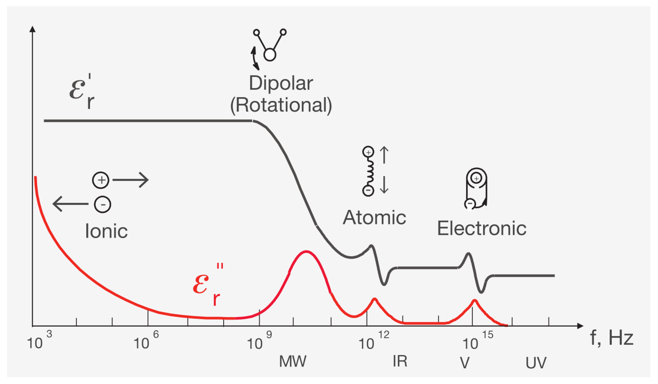
Figure 1 illustrates the basic concepts of dielectric property measurement. The real part, which is affected mainly by the water content, becomes dominant in the MHz range and the imaginary part of permittivity (or conductivity) of the soil has a high value in the KHz range and follows the 1/f behavior, as in [10,16].

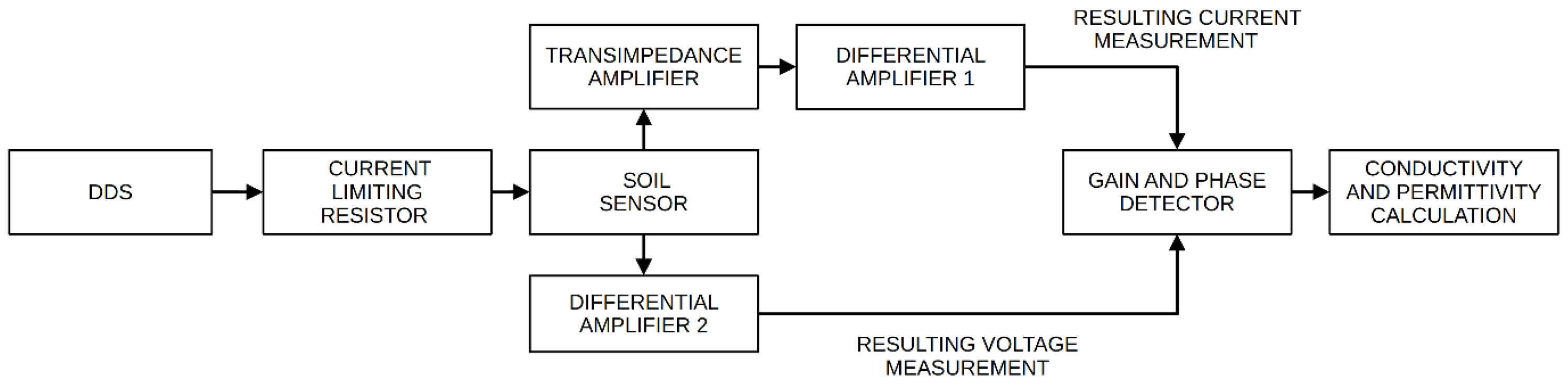
The measuring system of this work biases the soil with a sinusoidal signal through electrodes placed into it. Two different frequency ranges are used, to be able to measure both electric conductivity and water content. The signal passing through the soil changes in amplitude and phase due to the soil’s varying impedance. Then, the system measures the differential voltage across the soil’s impedance and the voltage of the amplifier. These two voltages are then fed into a module that can determine the amplitude gain and phase difference. Lastly, the system, using the amplitude gain and phase difference, calculates the impedance of the soil and then determines the conductivity and the water content. The block diagram of the system is shown in Figure 2.

The system consists of a Direct Digital Synthesis (DDS) module that produces a sinusoidal signal of different frequencies ranging from 100 KHz to 10 MHz, a current limiting resistor, electrodes (soil sensor), two differential amplifiers measuring the resulting voltage of the impedance of the soil and the voltage output of the transimpedance amplifier (it is also called auto-balancing circuit amplifier [7,15], current to voltage converter) and the gain and phase detector module.

As mentioned above, soil has dielectric properties. To analyze them, the soil is considered as a uniform material which can be modeled as a circuit of a resistor parallel to a capacitor. The equivalent circuit’s impedance is

$${\rm Z}=R\parallel C\iff Y=G+jB$$

(3)

where Z is the composite complex resistance of the soil, R is the resistor and C is the capacitor. If the composite resistance is converted to composite conductance (the inverse value of Z), Υ is the complex conductance of soil (admittance), G is the conductance and B is the susceptance.

The primary objective of the circuit is to measure two quantities, the soil’s differential voltage and the current flowing through it. The first quantity is the voltage V_SOIL which is measured by the differential amplifier 2.

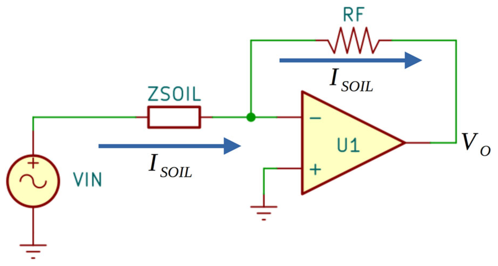
The current I_SOIL is measured by the transimpedance amplifier, which is shown in Figure 3. Its operation is to convert the current I_SOIL which is flowing through the unknown soil impedance Z_SOIL, into the voltage V_O, with the usage of R_F, as Equation (4) shows:

$$V_{\mathit{o}}=I_{SOIL}\cdot R_F$$

(4)

Another equation to describe the operation of the amplifier is:

$$V_{\mathit{o}}=\left(-{\displaystyle \frac{R_F}{Z_{SOIL}}}\right)\cdot V_{IN}$$

(5)

Solving Equation (5) for Z_SOIL, gives:

$$Z_{SOIL}=-{\displaystyle \frac{R_F}{V_{\mathit{o}}}}\cdot V_{IN}$$

(6)

Since admittance is the inverse of impedance, the value can be calculated using Equation (7):

$$Y_{SOIL}={\displaystyle \frac{1}{Z_{SOIL}}}=-{\displaystyle \frac{V_{\mathit{o}}}{R_F\cdot V_{IN}}}$$

(7)

To determine the real and imaginary components of the admittance separately, phase difference Δ_Φ between them is needed:

$$Y_{SOIL}=\left|Y_{SOIL}\right|\cdot \left(cos\left({\mathsf{\Delta }}_{\Phi }\right)+j\cdot sin\left({\mathsf{\Delta }}_{\Phi }\right)\right)$$

(8)

$$G=\left|Y_{SOIL}\right|\cdot cos\left({\mathsf{\Delta }}_{\Phi }\right)$$

(9)

$$B=\left|Y_{SOIL}\right|\cdot sin\left({\mathsf{\Delta }}_{\Phi }\right)$$

(10)

The real part of Y_SOIL is conductance G and the imaginary is susceptance B. These values are used to determine soil’s resistance R and capacitance C, as defined in the soil impedance equivalent circuit,

$$R={\displaystyle \frac{1}{G}}$$

(11)

$$C={\displaystyle \frac{B}{\omega }}$$

(12)

where ω is the angular velocity of the signal.

The last values can be used to determine soil’s dielectric properties, specifically the apparent electrical conductivity EC_α and the relative permittivity ε_r, both at the measured temperature T (°C), as shown below:

$${EC}_{\alpha }={\displaystyle \frac{1}{R}}\cdot k_g$$

(13)

$${\epsilon }_r={\displaystyle \frac{C}{{\epsilon }_0\cdot k_g}}$$

(14)

where k_g is the electrode geometry factor [8,17], ε₀ is the vacuum permittivity (electric constant), ε_r is the relative permittivity of the soil and EC_α is the apparent electrical conductivity of soil. A detailed description for the electrode geometry factor k_g can be found in the Measurement Setup Section.

In most cases, the apparent EC_{25 °C} and relative permittivity ε_{r25 °C} for temperature 25 °C is used, which are calculated with the temperature coefficient f_T [7,11] and are shown below,

$${EC}_{25 °\mathrm{C}}={EC}_{\alpha }\cdot f_T$$

(15)

$$f_T=0.4470+1.4034·exp\left(-{\displaystyle \frac{T}{26.815 °\mathrm{C}}}\right)$$

(16)

$${\epsilon }_r={\epsilon }_r+0.114·(25-T)$$

(17)

where T is the temperature in degrees Celsius.

2.2. Circuit Analysis

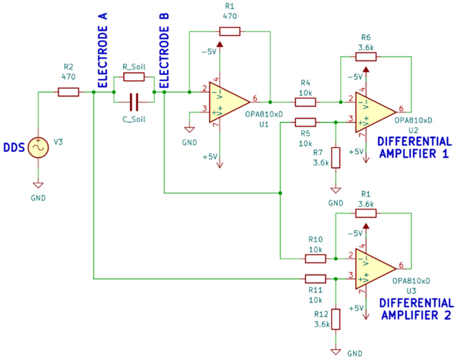
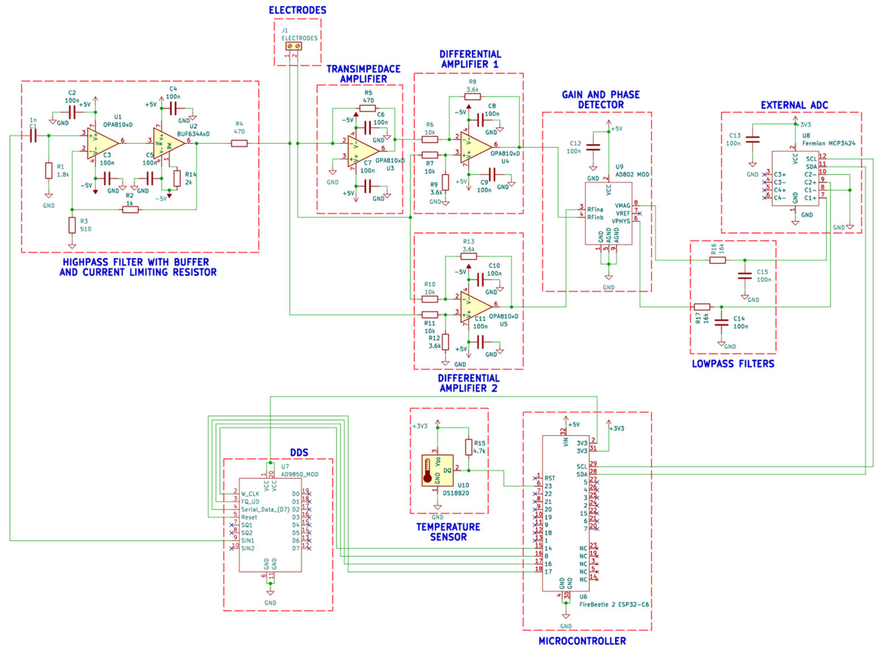
Figure 4 shows a simplified version of the circuit that was used to determine soil properties. It is based on [7,15]. The voltage source V3 = 2 Vpp represents the Direct Digital Synthesis module (DDS) that produces the sinusoidal signal applied to soil electrodes. U1 is the inverting transimpedance amplifier with a gain depending on the soil’s impedance. R2 is the current limiting resistor that also provides greater stability to the system as a whole, according to [11,15] and the conclusions derived through the design and the measurements of this circuit. R_Soil and C_Soil represent the soil’s resistance and capacitance respectively. R1 is the feedback resistor that determines the amplifier gain. The resistor R1 and R2 values, for stability reasons [15], should be equal. After experimental measurements during design stage, the chosen values were R1 = R2 = 470 Ω, which gave noise-free and stable measurements. Expecting form initial measurements on the soil to have a resistance approximately in the range 100–2000 Ω, a capacitance in the range pF to tens of nF and the signal frequence to rise up to MHz, the initial testing values for R1 and R2 were chosen from Table 2-1 of [15], according to the expected values of columns 1 and 2 (R = 100 Ω and 5 kΩ, where the measured capacitance is expected from tens of pF and up to 1 μF). After testing, the low R1 value producing noise-free measurements was found at 470 Ω.

U2 is the differential amplifier that outputs the voltage Vo due to the current through the soil and U3 is the differential amplifier that outputs the voltage Vx due to the voltage across the soil’s impedance. The gain on both amplifiers is equal to 0.36, which is necessary to protect the next stage, which is the gain and phase detector module.

Equation (7) becomes:

$$\left|Y_{SOIL}\right|=-{\displaystyle \frac{V_{\mathit{o}}}{R_F\cdot V_x}}$$

(18)

Figure 5 presents a more detailed schematic of the system. The sinusoidal bias signal is generated by the programmable DDS AD9850. The signal then passes through an active RC high-pass filter with a cutoff frequency of 95 kHz to suppress the DC component of the DDS output. This subcircuit has a gain of 1.1. The AD8302 module is a gain and phase detector that receives two signals of the same frequency and provides output voltages proportional to their phase difference and amplitude ratio [18]. The resulting signals (Vmag and Vphase) are DC voltages that pass through low-pass filters with a cutoff frequency of 100 Hz. After the filters, the DC signal levels are measured by the external ADC MCP3424. The temperature which is needed for correction is sensed by a digital temperature sensor DS18B20. The microcontroller that controls the DDS and reads the output signals is the FireBeetle 2 ESP32-C6.

2.3. Simulation Results

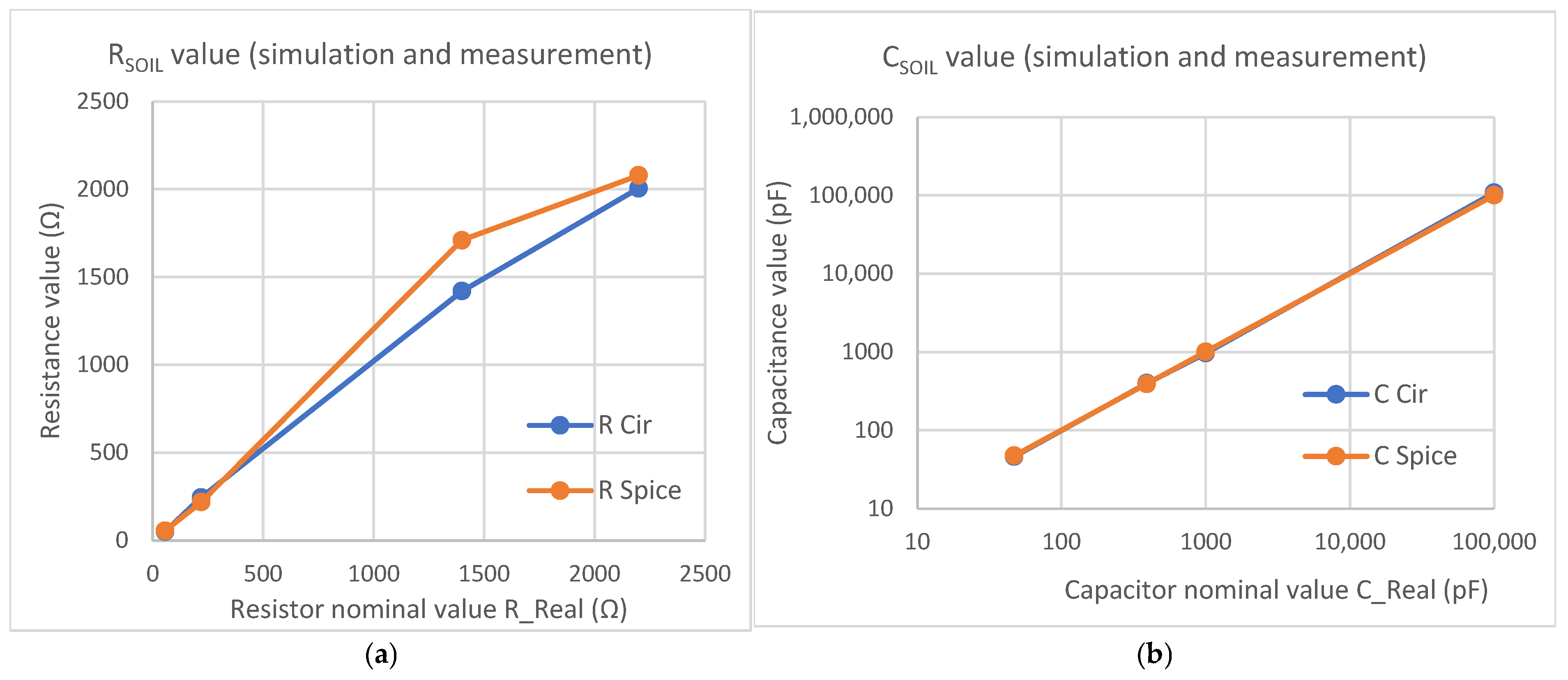
The circuit of Figure 4 was simulated in LTSpice 24.1.5 and compared with measurements taken in the laboratory with discrete components, to determine the correct operation of the system. The results of four different pairs of components are presented in

Table 1. Discrete components test results.

R Real (Ω)	C Real (F)	R Cir (Ω)	C Cir (F)	R Spice (Ω)	C Spice (F)	Error R-C (%)	Error R-S (%)	Error C-S (%)
2200 Ω	100 nF	2006 Ω	108 nF	2079 Ω	100.36 nF	8.8–8.0	5.5–0.4	3.6–7.1
220 Ω	390 pF	246 Ω	399 pF	219 Ω	391.4 pF	11.7–2.3	0.6–0.4	11.0–1.9
1400 Ω	47 pF	1420 Ω	46.2 pF	1710 KΩ	47.4 pF	1.4–1.7	22.1–0.9	20.4–2.6
56 Ω	1 nF	50 Ω	0.969 nF	56 Ω	1.004 nF	9.6–3.1	0.2–0.4	10.5–3.6

and Figure 6.

The first two columns (R Real and C Real) have the actual values of the discrete components that were used to make the soil impedance in the laboratory. The third and fourth columns (R Cir and C Cir) are the values that were calculated with the circuit and were expected to give a value very close to the R Real and C Real values of the discrete components that form the soil’s impedance. The fifth and sixth columns (R Spice and C Spice) are the values calculated through the circuit simulation with LTspice 24.1.5 software. The seventh column shows the error between the actual and the circuit’s values, the eighth has the error between the actual and the simulation’s values and the last one has the error between the circuit’s and the simulation’s values.

Table 2. Mean error discrete components test results.

	Mean Error R-C (%)	Mean Error R-S (%)	Mean Error C-S (%)
Mean Error R	7.9	7.1	11.4
Mean Error C	3.8	0.5	3.8

shows the resulting mean errors, with the first line showing the error of the resistances and the second the error of the capacitances.

The calculated results from the laboratory measurements and the simulation are close to the actual values and deviate mainly for values outside the typical range encountered in soil measurements (if we measured them without converting them to Equations (13) and (14).

2.4. Measurement Setup

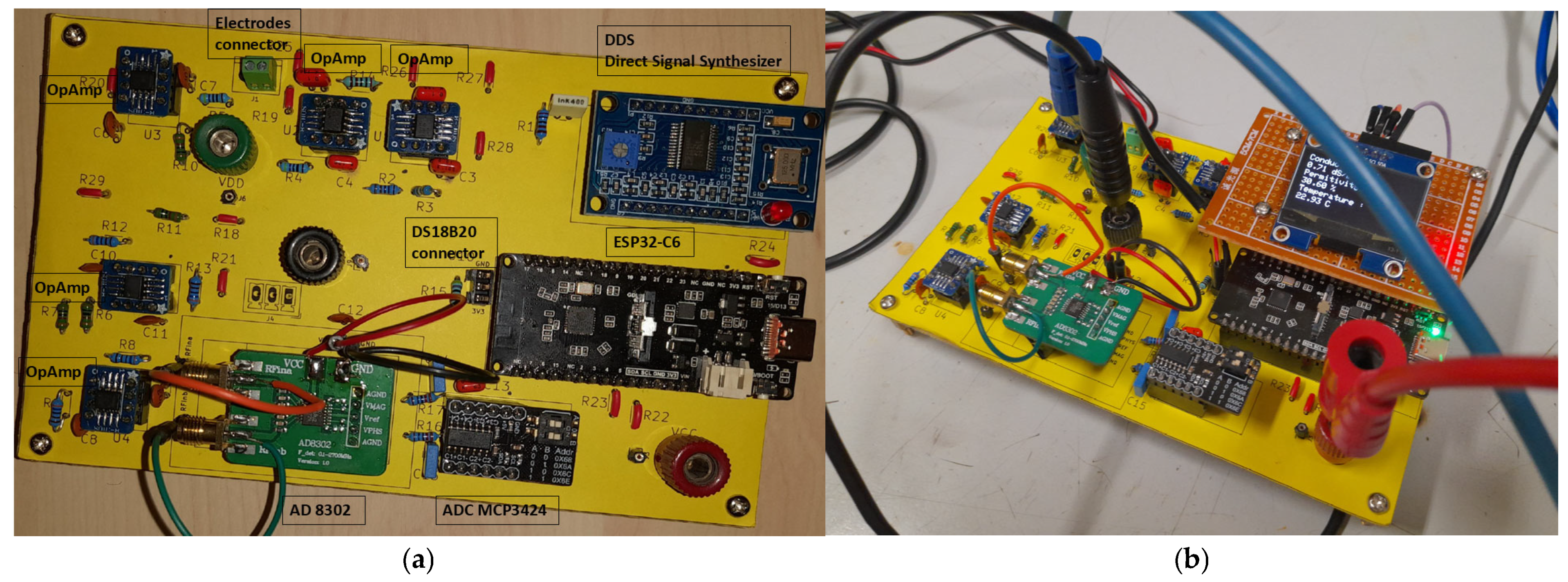
To verify the correct operation of the sensor, measurements were taken from three different soils, at room temperature 20 °C, with the system shown in Figure 7:

• Soil sample A, sandy type;
• Soil sample B, sandy–clay type;
• Soil sample C, sandy–loamy type.

And, in two soil moisture conditions:

• Addition of water without mixing, where water was added without mixing to simulate field conditions after irrigation or rainfall.
• Addition of water with mixing, where the water is mixed sufficiently with the soil to simulate homogeneous saturation conditions.

The signal was set at frequencies 100 kHz, 150 kHz, 200 kHz, 9 MHz, 9.5 MHz and 10 MHz. Then, the measurements at the first three frequencies were averaged for EC_a estimation, whereas those at the last three frequencies were averaged for VWC estimation. These frequencies are used to achieve better discrimination between the kHz and MHz frequency ranges, so that we could obtain greater influences from the real part in kHz and the imaginary part in MHz for the calculation of the impedance. The measurements were taken at a temperature approximately at 20–25 °C. All the results are converted for EC_α and e_r at 25 °C, as is used in the literature, without changing the variable index, due to the negligible difference.

Figure 7. Circuit board of the sensor. (a) The components of the circuit and the connectors are shown. The OpAmps, the electrode connector, and the DDS are placed on the upper part, while the magnitude-phase comparator (AD8302), the ADC MCP and the ESP32-C6 are placed below. At the left side of ESP32 is placed the connector of the temperature sensor DS18B20. (b) The sensor during operation, with LCD display on the upper right corner.

Figure 7. Circuit board of the sensor. (a) The components of the circuit and the connectors are shown. The OpAmps, the electrode connector, and the DDS are placed on the upper part, while the magnitude-phase comparator (AD8302), the ADC MCP and the ESP32-C6 are placed below. At the left side of ESP32 is placed the connector of the temperature sensor DS18B20. (b) The sensor during operation, with LCD display on the upper right corner.

Two different water quantities, 330 mL and 660 mL, were chosen to be added to the soil, instead of smaller quantities, because they produced more clearly distinguishable results in measuring the condition of the soil. With the specified water quantities, the soil is simulated in conditions nearly dry (after many days without rain) and nearly saturated (after rainfall) or saturated [19]. The dry soil sample weights used in the experiments were approximately 2.8 kg each, measured after 24 h heating in oven, at temperature 105 °C. Finally, the results were compared with a commercial meter, the Meter 5TE [20], whose measurements were used as reference values.

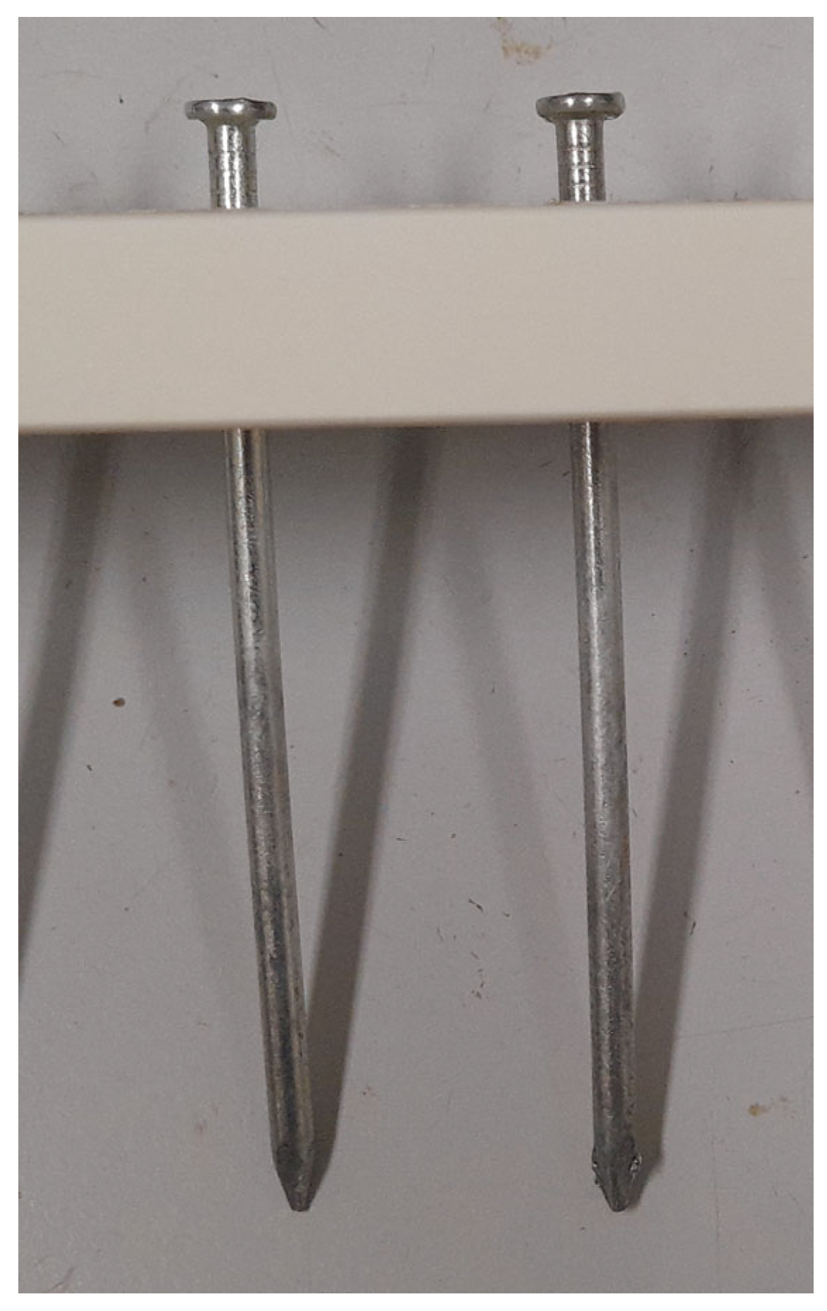
The electrodes consist of two nails mounted on a chipboard plate with melamine surface. The nails are made of galvanized hard steel to protect against corrosion and rust. The distance between them is 3 cm, the total length is 10 cm, the length in contact with the soil is 7 cm and the nail diameter is 4 mm. As mentioned above, k_g is the term associated with the geometry of the electrodes. This term is necessary for converting the measured conductivity and capacitance into soil EC_a and relative soil permittivity.

The term is calculated either empirically or by solving Gauss’s equations. The calculation for the geometric factor k_g of this sensor is based on [8,21], and is given as:

$$k_g={\displaystyle \frac{1}{\pi \cdot L}}\cdot ln\left({\displaystyle \frac{2\cdot a}{r}}-1\right)\approx 0.1697 {\mathrm{c}\mathrm{m}}^{-1}$$

(19)

where L is the length of the electrode that comes into contact with the ground, a is the distance between the electrodes and r is the radius of the electrodes.

The initial idea for the electrodes shown in Figure 8 was to use them temporarily, to conduct an initial study and then construct electrodes that could be buried in the soil. However, this was not implemented because the current design was easy to use and showed minimal oxidation, due to the galvanized steel’s resistance to oxidation.

The total hardware cost of the sensor was only 60 €, consisting of the DS18B20 (2.5 €), the DDSS AD9850 (10 €), the ESP32-C6 (6 €), the ADC MCP3424 (7 €), the OPA 810 (4 × 5 €) the AD8302 (13 €) and the electrodes (approximately 2 €).

3. Results

The following

Table 3. Sample A results.

Sample Preparation	Water (mL)	Circuit ECa (mS/cm)	Circuit VWC (%)	ECa Meter (mS/cm)	VWC Meter (%)	ECa Error (%)	VWC Error (%)
Without mixing	330	0.19	13.7	0.22	12.0	15.5	14.8
	660	0.08	15.2	0.12	11.5	36.7	32.3
With mixing	330	0.50	17.8	0.56	22.7	9.7	21.4
	660	0.67	25.3	0.66	27.0	1.2	6.5

,

Table 4. Sample B results.

Sample Preparation	Water (mL)	Circuit ECa (mS/cm)	Circuit VWC (%)	ECa Meter (mS/cm)	VWC Meter (%)	ECa Error (%)	VWC Error (%)
Without mixing	330	0.34	36.0	0.49	21.3	30.8	68.9
	660	0.17	15.8	0.18	12.9	8.8	22.8
With mixing	330	0.45	16.7	0.67	22.2	33.2	24.6
	660	0.75	24.8	0.59	20.8	26.3	19.2

and

Table 5. Sample C results.

Sample Preparation	Water (mL)	Circuit ECa (mS/cm)	Circuit VWC (%)	ECa Meter (mS/cm)	VWC Meter (%)	ECa Error (%)	VWC Error (%)
Without mixing	330	0.24	10.0	0.22	11.4	9.5	12.6
	660	0.11	14.2	0.10	10.9	13.7	30.3
With mixing	330	0.11	18.7	0.12	21.6	4.3	13.4
	660	0.29	14.2	0.25	14.8	14.6	3.7

present the measurements of EC_a and VWC of the three soil samples, converted for 25 °C. The first column of the tables shows the soil condition, the second column shows the amount of water in each condition, the third and fourth columns show the EC_a and VWC values measured by the circuit, the fifth and sixth columns show EC_a and VWC measured by the Meter 5TE instrument and the last two columns show the error between the circuit and the Meter 5TE.

Table 6. Overall error of each state.

Sample Preparation	Water (mL)	Mean Error ECa (%)	Mean Error VWC (%)
Without mixing	330	18.6	32.1
	660	17.0	28.5
With mixing	330	15.7	19.8
	660	14.0	9.8

shows the overall error of each state and measurement type and

Table 7. Overall error of the sensor.

Mean Error ECa (%)	Mean Error VWC (%)	Mean Error of the System (%)
16.3	24.2	20.2

shows the overall error of the system as a whole, without calibration on any soil type.

Summarizing this section, this sensor is not more accurate than all low-cost sensors, but it has the advantage of measuring EC_a and VWC with a dual-frequency approach and good accuracy without special calibration per soil type, with a simple and low-cost circuit.

Table 8. Different methods’ accuracy comparison.

Study	Measured Parameters	Method/Reference	Reported Accuracy
Rêgo Segundo et al. [7]	VWC, ECα, temperature	Auto-balancing bridge, calibrated models	RMSE ≈ 0.002 m3/m3 for VWC in lab; temperature correction improved EC estimation
Okasha et al. [12]	VWC	Low-cost capacitive sensor	R2 = 0.967, RMSE = 0.014
Teletos et al. [14]	ECα, VWC, temperature	AC bipolar pulse, impedance analyzer benchmark	Mean EC error 8.95–9.98%
This sensor	ECα, VWC, temperature	Dual-frequency impedance, 5TE comparison	Mean error: 16.3% ECa, 24.2% VWC, 20.2% overall, without soil-specific calibration

shows a comparison of accuracy between this sensor and other systems.

Previous systems based on auto-balancing bridge or calibrated capacitive approaches achieved lower RMSE values for VWC estimation, while recent low-cost EC systems reported mean EC errors below 10%. However, these systems often rely on specific calibration models, controlled laboratory conditions, a limited number of soil types or focus mainly on one parameter. In contrast, the present system estimates both ECa and VWC using two different frequency ranges and was evaluated on three soil types and two moisture preparation conditions without soil-specific calibration. The main advantage of the proposed approach is not absolute accuracy, but the combination of low cost, simple implementation, dual-parameter estimation and applicability as a preliminary soil monitoring tool to help farmers use precision agriculture with low cost.

4. Conclusions

This work presents the design and experimental evaluation of a sensor estimating soil moisture and electrical conductivity. The system uses dual-frequency measurements (kHz for EC_α/MHz for VWC), synchronous temperature compensation and has an ultra-low hardware cost (~60 €). The combination of the above characteristics (dual-frequency, temperature measurement and very low-budget with simple electrode structure) for soil properties measurements is the innovation of the sensor.

The use of the sensor without calibration shows a mean error approximately above 15% in most cases and limits the scope of application for low-budget on-field quick estimations. The experimental evaluation has taken place in three soil types, room temperature and two moisture levels and cannot be universally applicable without further measurements. If calibration is applied, the mean error is expected to drop dramatically, and this sensor can be a helpful tool for precision agriculture.

The results indicate that the mean measurement error typically remained approximately above 15%, except in a few cases. This can be attributed to several factors encountered during the experiments and implementation of the system, and these are analyzed below.

The first error source identified was the contact of the electrodes with the soil. As mentioned above, the electrodes are galvanized steel nails placed in a chipboard. The electrode structure did not exert sufficient surface pressure on the soil to ensure a better or reproducible interface between the soil and the electrode. Also, if the electrodes were not placed vertically or moved during the measurements, the result was poor contact and therefore incorrect measurements. This problem became even more pronounced at the measurements on soil samples B and C because they are loamy and clayey, respectively, so they kept their shape better in the test containers and held the water that was added, in accordance with findings in [19]. In other words, if the electrodes of the system or the electrodes of Meter 5TE instrument were removed from the soil, then these could not return to its original state and have the same good contact with soil. The issue was mitigated by compacting the soil (for measuring mixed soil) on one side of the container so that gaps between the electrodes and the soil were reduced. Another method of fixing this error could be to repeat mixing the soil and repositioning the electrodes in a uniform soil.

Another error source was the slowly degrading waterproof protection of the electrode board. At the beginning of the experiments, there was no problem, but as time went by, moisture passed silently through the particle board and created small problems in the measurements. Although no issues were initially observed, moisture inside the particle board of the electrodes was, over time, compromising the integrity of the measurements. A sufficient way to handle this problem could be the use of a thick plastic layer instead of a chipboard.

During the experiments, it was found the significant influence of mixing time and method, i.e., the same soil samples that had been mixed quickly or not thoroughly (only superficially or partially) were not homogeneous, resulting in changes in the measurements between them. As mentioned above, depending on the type of sample, clay and loamy soils did not mix easily. The experimental data are exactly as acquired during the measurements, without “corrections” or “improvements” and clearly show the existence or greater error on these samples having “Without mixing” preparation. This soil preparation state is more similar to the actual condition of the soil in the fields.

Another error was the noise induced in the cable type. The flat cables that were used for wiring the electrodes cannot keep the signal noise-free. Also, the small distance between the two leads reduced the circuit’s performance, especially at high frequencies. A significant improvement can be achieved by changing the wiring of the electrodes to coaxial type with minimum length and the connectors to RF type, so that the shielding can reduce the noise. Additionally, soldering the components on the printed circuit board and avoiding the connectors could minimize the parasitic capacitances and improve the measurements in high frequency range.

Another important factor affecting measurement is calibration. As calibration is required in most soil measurements systems [22,23], it is also necessary for this circuit to achieve accurate measurements. Different soil types have different chemical, physical and electrical properties. During the use of commercial soil properties meters, the user must configure the meter central unit to the correct soil type so that the appropriate parameters are used during calculations, or they must calibrate the minimum and maximum range values [24,25].

Another problem that contributed to the final error had to do with the construction and programming of the system. During the calculations performed by the microcontroller, DDS receives the frequency from stored variables. As mentioned, the DDS module is not able to output the exact frequency that is sent by the microcontroller, resulting in small errors in the calculation of the angular velocity. The quantization frequency error [26] is lower than 1 Hz, but the crystal error driving the DDS is usually 50 ppm.

In summary, the system achieved an average error above 15% in most cases and 20% in some cases, demonstrating that it can provide a satisfactory initial assessment of soil conditions, particularly in applications where low complexity and low cost are decisive factors. The results show that, despite its accuracy limitations, the proposed solution can serve as a support tool in agricultural applications, contributing to decision-making on irrigation and crop management. At the same time, it is recognized that the error rate limits the use of the system in cases where high accuracy is required. Although high accuracy is not necessary every day in the field, an effortless improvement is a calibration on the specific soil type, which can elevate significantly the system’s accuracy.

References

1. Manono, B.O.; Mwami, B.; Mutavi, S.; Nzilu, F. Precision Farming with Smart Sensors: Current State, Challenges and Future Outlook. Sensors 2026, 26, 882. [Google Scholar] [CrossRef] [PubMed]
2. Song, W.; Li, X.; Zhang, J.; Huang, J.; Wang, J.; Feng, W.; Guo, Y.; Ren, L. Soil Sensors in Smart Agriculture: Multi-Type Monitoring Technologies and Ecological Development Pathways. Agriculture 2026, 16, 359. [Google Scholar] [CrossRef]
3. Tsiropoulos, Z.; Skoubris, E.; Fountas, S.; Gravalos, I.; Gemtos, T. Development of an Energy Efficient and Fully Autonomous Low-Cost IoT System for Irrigation Scheduling in Water-Scarce Areas Using Different Water Sources. Agriculture 2022, 12, 1044. [Google Scholar] [CrossRef]
4. Fragkou, E.; Tsegas, G.; Karagkounis, A.; Moussiopoulos, N. Quantifying the impact of a smart farming system application on local-scale air quality of smallhold farms in Greece. Air Qual. Atmos. Health 2023, 16, 1–14. [Google Scholar] [CrossRef]
5. Cuéllar Torres, F.A.; Colorado Montaño, J.D.; Narducci Marín, M.S. Design, Manufacturing, and Calibration of a Conductivity Sensor for Precision Agriculture. In Proceedings of the 2023 IEEE Colombian Caribbean Conference (C3), Barranquilla, Colombia, 22–25 November 2023; pp. 1–5. [Google Scholar] [CrossRef]
6. Hilhorst, M. Dielectric Characterisation of Soil. Ph.D. Thesis, Agricultural University of Wageningen, Wageningen, The Netherlands, 1998. [Google Scholar]
7. Rêgo Segundo, A.K.; Martins, J.H.; Monteiro, P.M.d.B.; de Oliveira, R.A.; Freitas, G.M. A novel low-cost instrumentation system for measuring the water content and apparent electrical conductivity of soils. Sensors 2015, 15, 25546–25563. [Google Scholar] [CrossRef] [PubMed]
8. Thring, R.W.; Bicalho, K.V.; Ng, C.W.W. Factors affecting soil permittivity and proposals to obtain gravimetric water content from time domain reflectometry. Can. Geotech. J. 2014, 51, 1308–1317. [Google Scholar] [CrossRef]
9. Corwin, D.; Yemoto, K. Salinity: Electrical Conductivity and Total Dissolved Solids. Methods Soil Anal. 2017, 10. [Google Scholar] [CrossRef]
10. Keysight Technologies. Basics of Measuring the Dielectric Properties of Materials. Available online: https://www.keysight.com/zz/en/assets/7018-01284/application-notes/5989-2589.pdf (accessed on 20 March 2026).
11. Rhoades, J.D.; Chanduvi, F.; Lesch, S. Soil Salinity Assessment: Methods and Interpretation of Electrical Conductivity Measurements; Irrigation and Drainage Paper 57; FAO: Rome, Italy, 1999. [Google Scholar]
12. Okasha, A.M.; Ibrahim, H.G.; Elmetwalli, A.H.; Khedher, K.M.; Yaseen, Z.M.; Elsayed, S. Designing low-cost capacitive-based soil moisture sensor and smart monitoring unit operated by solar cells for greenhouse irrigation management. Sensors 2021, 21, 5387. [Google Scholar] [CrossRef] [PubMed]
13. da Silva, M.J.; Schleicher, E.; Hampel, U. A novel needle probe based on high-speed complex permittivity measurements for investigation of dynamic fluid flows. IEEE Trans. Instrum. Meas. 2007, 56, 1249–1256. [Google Scholar] [CrossRef]
14. Teletos, E.; Tsiakmakis, K.; Hatzopoulos, A.T.; Stefanou, S. Development of a Low-Cost Measurement System for Soil Electrical Conductivity and Water Content. AgriEngineering 2025, 7, 329. [Google Scholar] [CrossRef]
15. Texas Instruments. TIDA-060029 LCR Meter Analog Front End Reference Design. Available online: https://www.ti.com/lit/pdf/TIDUEU6 (accessed on 20 March 2026).
16. Hilhorst, M.A. A pore water conductivity sensor. Soil Sci. Soc. Am. J. 2000, 64, 1922–1925. [Google Scholar] [CrossRef]
17. Mosaic Industries. Cell Constant of Parallel Wire Electrodes: Solving Gauss’s Law Electric Field Equations for a Paraxial Two-Electrode Conductivity Cell. Available online: https://www.mosaic-industries.com/embedded-systems/instrumentation/conductivity-meter/two-electrode-cell-constant (accessed on 20 March 2026).
18. Analog Devices. AD8302: LF–2.7 GHz RF/IF Gain and Phase Detector Data Sheet. Available online: https://www.analog.com/media/en/technical-documentation/data-sheets/AD8302.pdf (accessed on 20 March 2026).
19. Decagon Devices, Inc. 5TE Water Content, EC and Temperature Sensors Operator’s Manual, Version 2. Available online: https://publications.metergroup.com/Manuals/20435_5TE_Manual_Web.pdf (accessed on 20 March 2026).
20. Hong, C.-H.; Chong, S.-H.; Cho, G.-C. Theoretical study on geometries of electrodes in laboratory electrical resistivity measurement. Appl. Sci. 2019, 9, 4167. [Google Scholar] [CrossRef]
21. Koufogeorgos, V.D.; Hatzopoulos, A.T.; Tsiakmakis, K.; Vassios, V.; Papadopoulou, M.S.; Papakostas, D.K. Design and Development of a Low-Cost Circuit for Soil Electrical Conductivity Measurement Using the Wenner Array Method. In Proceedings of the 2025 14th International Conference on Modern Circuits and Systems Technologies (MOCAST 2025), Dresden, Germany, 11–13 June 2025. [Google Scholar] [CrossRef]
22. METER Group. TEROS 11/12 User Manual; METER Group, Inc.: Pullman, WA, USA, 2018; Available online: https://www.misure.net/sites/default/files/pdf/20587_TEROS11-12_Manual_Web.pdf (accessed on 24 April 2026).
23. Hanna Instruments. HI98331 GroLine Direct Soil Conductivity and Temperature Tester Instruction Manual; Hanna Instruments, Inc.: Woonsocket, RI, USA, 2021; Available online: https://www.documentation.hannainst.com/manuals/download/1430 (accessed on 24 April 2026).
24. Starr, J.L.; Paltineanu, I.C. Methods for Measurement of Soil Water Content: Capacitance Devices. In Methods of Soil Analysis: Part 4 Physical Methods; Dane, J.H., Topp, G.C., Eds.; SSSA Book Series No. 5; Soil Science Society of America: Madison, WI, USA, 2002; pp. 463–474. [Google Scholar]
25. Rhoades, J.D. Electrical Conductivity and Soil Salinity. In Methods of Soil Analysis: Part 3 Chemical Methods; Sparks, D.L., Ed.; SSSA Book Series No. 5; Soil Science Society of America: Madison, WI, USA, 1996; pp. 417–435. [Google Scholar]
26. Analog Devices. CMOS 125 MHz Complete DDS Synthesizer AD9850 Datasheet; Analog Devices, Inc.: Norwood, MA, USA, 2004; Available online: https://www.analog.com/media/en/technical-documentation/data-sheets/AD9850.pdf (accessed on 26 April 2026).
Figure 1. Basics of measuring the dielectric properties of materials [10]. When examining the dielectric behavior of materials, in the low frequency range the ionic conduction and the dipole orientation mechanisms prevail, while in the high frequency range the atomic and electronic mechanisms prevail. At low frequencies, ionic conductivity is the most prevalent in moist materials.
Electronics 15 02089 g001
Figure 2. Block diagram of the experimental setup.
Electronics 15 02089 g002
Figure 3. Basic circuit of a transimpedance amplifier.
Electronics 15 02089 g003
Figure 4. Simplified circuit schematic.
Electronics 15 02089 g004
Figure 5. Detailed circuit schematic.
Electronics 15 02089 g005
Figure 6. The values (simulated and measured with circuit) of soil resistance (a) and capacitance (b) vs. their nominal value of the discrete components used.
Electronics 15 02089 g006
Figure 8. The electrodes are 10 cm Φ 4 mm galvanized steel nails on chipboard plate.
Electronics 15 02089 g008