Author Contributions
Conceptualization, Y.W., X.Q. and K.Z.; Methodology, X.Q. and K.Z.; Software, Y.W. and J.S.; Validation, Y.W. and J.S.; Formal Analysis, X.Q. and K.Z.; Investigation, Y.W.; Resources, X.Q. and K.Z.; Data Curation, Y.W. and J.S.; Writing—Original Draft Preparation, Y.W.; Writing—Review and Editing, Y.W., X.Q., J.S. and K.Z.; Visualization, Y.W. and J.S.; Supervision, X.Q. and K.Z.; Project Administration, Y.W.; Funding Acquisition, X.Q. and K.Z. All authors have read and agreed to the published version of the manuscript.
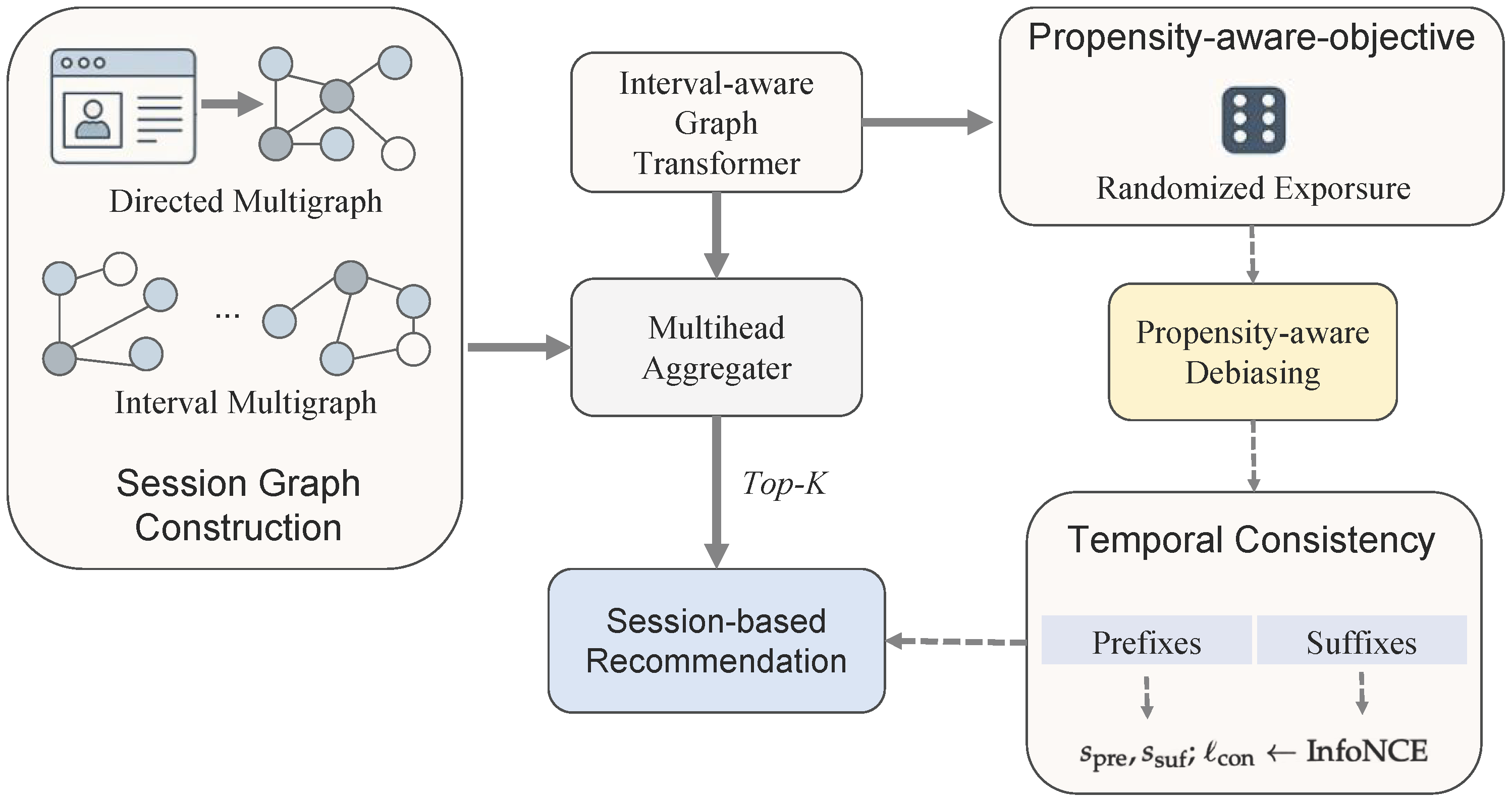
Figure 1.
The end-to-end framework illustrating session graph construction, the interval-aware graph transformer, propensity-aware objective, and temporal consistency module.
Figure 1.
The end-to-end framework illustrating session graph construction, the interval-aware graph transformer, propensity-aware objective, and temporal consistency module.
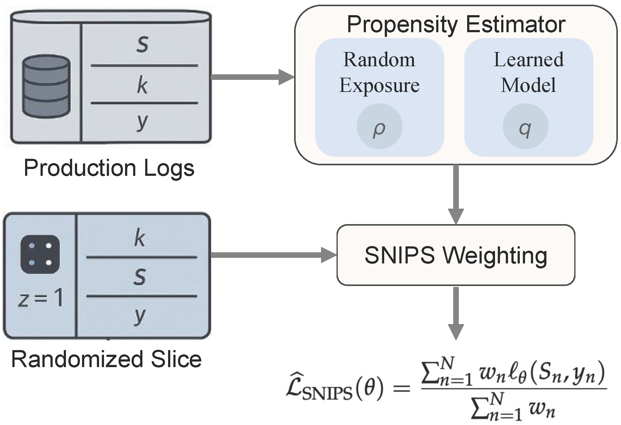
Figure 2.
The propensity-aware learning flow, showing propensity estimation from randomized logs and the application of SNIPS weighting.
Figure 2.
The propensity-aware learning flow, showing propensity estimation from randomized logs and the application of SNIPS weighting.
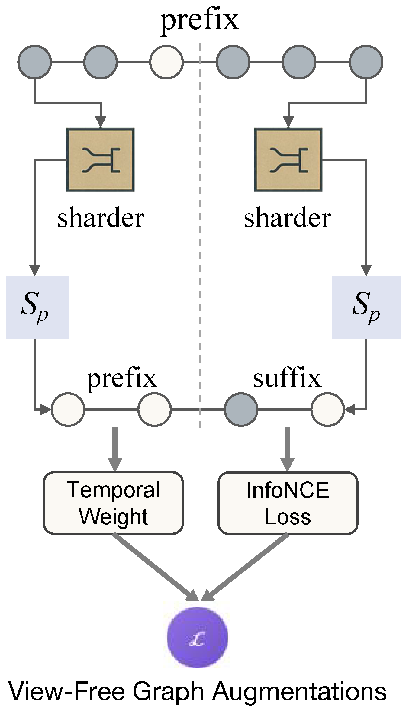
Figure 3.
The view-free temporal consistency mechanism, showing the prefix–suffix split, temporal decay weighting, and contrastive alignment.
Figure 3.
The view-free temporal consistency mechanism, showing the prefix–suffix split, temporal decay weighting, and contrastive alignment.
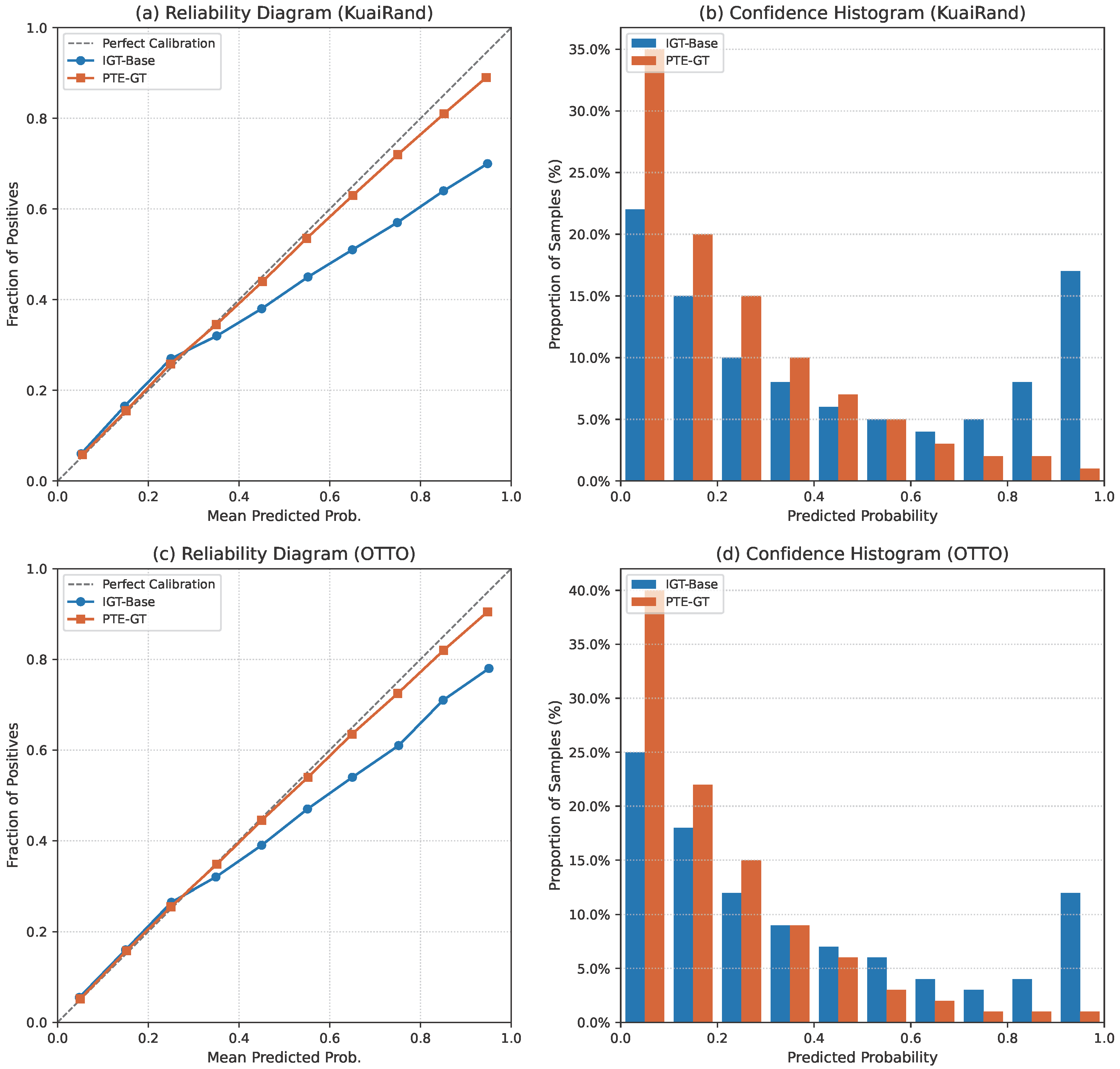
Figure 4.
Comprehensive calibration analysis on KuaiRand and OTTO. (a,c) Reliability diagrams comparing IGT-Base and PTE-GT; the diagonal (dashed line) represents perfect calibration. (b,d) Histograms of predicted confidence for ground-truth items, illustrating that PTE-GT avoids the overconfidence of the baseline.
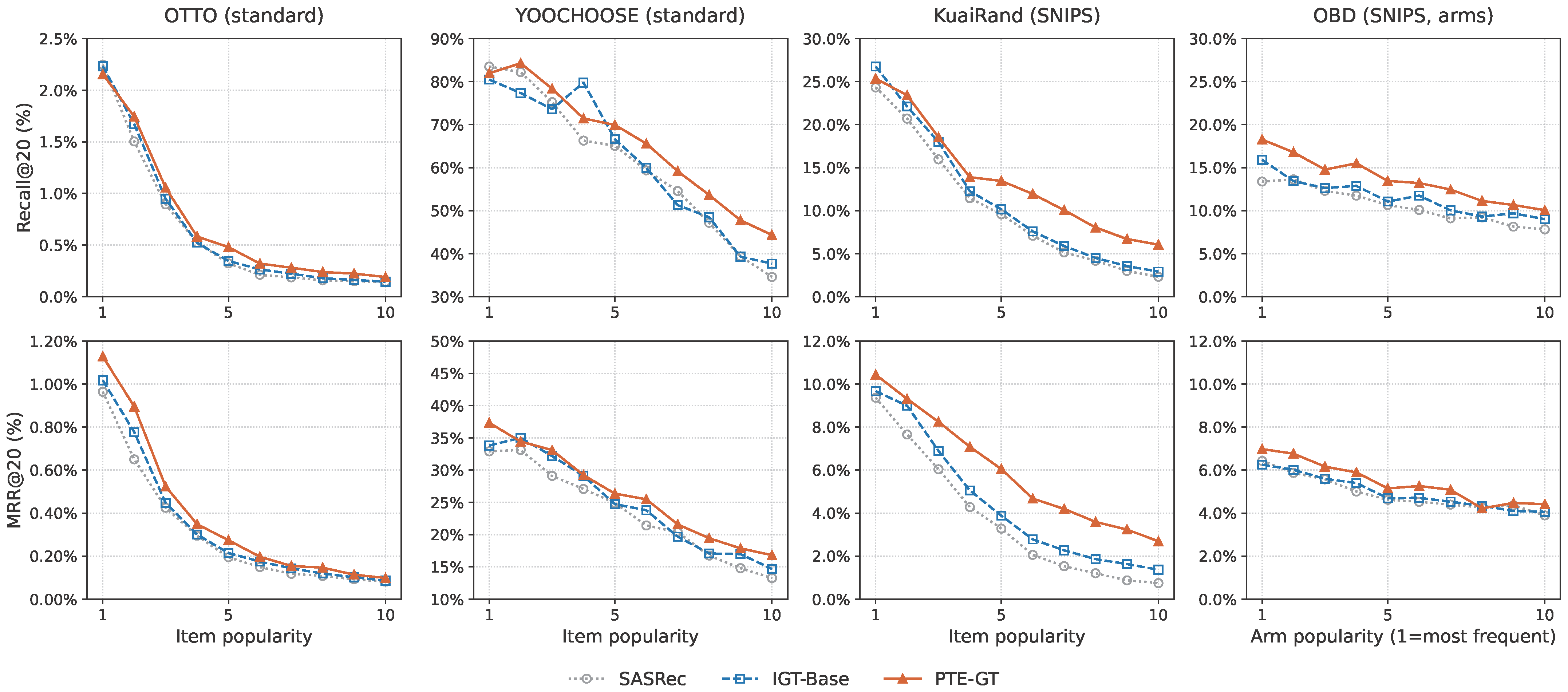
Figure 5.
Comprehensive analysis of long-tail performance across item popularity deciles (1 = most popular, 10 = long-tail). (Top row) shows Recall@20. (Bottom row) shows MRR@20.
Figure 5.
Comprehensive analysis of long-tail performance across item popularity deciles (1 = most popular, 10 = long-tail). (Top row) shows Recall@20. (Bottom row) shows MRR@20.
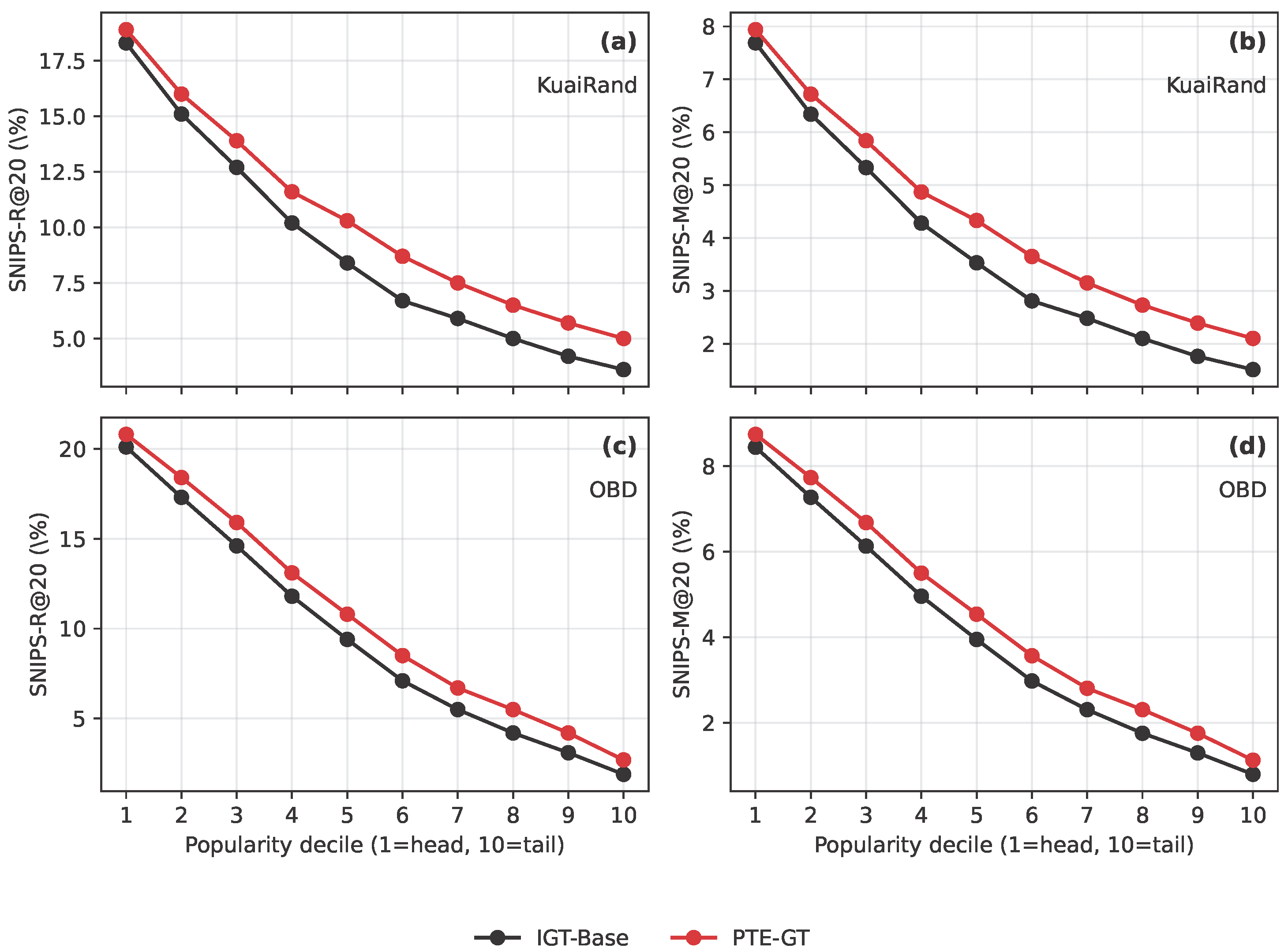
Figure 6.
SNIPS-weighted long-tail performance by item popularity decile on KuaiRand (KuaiRand) and OBD (OBD). The figure reports SNIPS-R@20 and SNIPS-M@20 across popularity deciles.
Figure 6.
SNIPS-weighted long-tail performance by item popularity decile on KuaiRand (KuaiRand) and OBD (OBD). The figure reports SNIPS-R@20 and SNIPS-M@20 across popularity deciles.
Figure 7.
Component-wise ablation on KuaiRand and OTTO. Panel (a) shows mean SNIPS-R@20 on KuaiRand, panel (b) shows SNIPS-R@20 on the bottom 60% least popular items on KuaiRand (long-tail), and panel (c) shows standard R@20 on OTTO. Error bars indicate the standard deviation over five runs.
Figure 7.
Component-wise ablation on KuaiRand and OTTO. Panel (a) shows mean SNIPS-R@20 on KuaiRand, panel (b) shows SNIPS-R@20 on the bottom 60% least popular items on KuaiRand (long-tail), and panel (c) shows standard R@20 on OTTO. Error bars indicate the standard deviation over five runs.
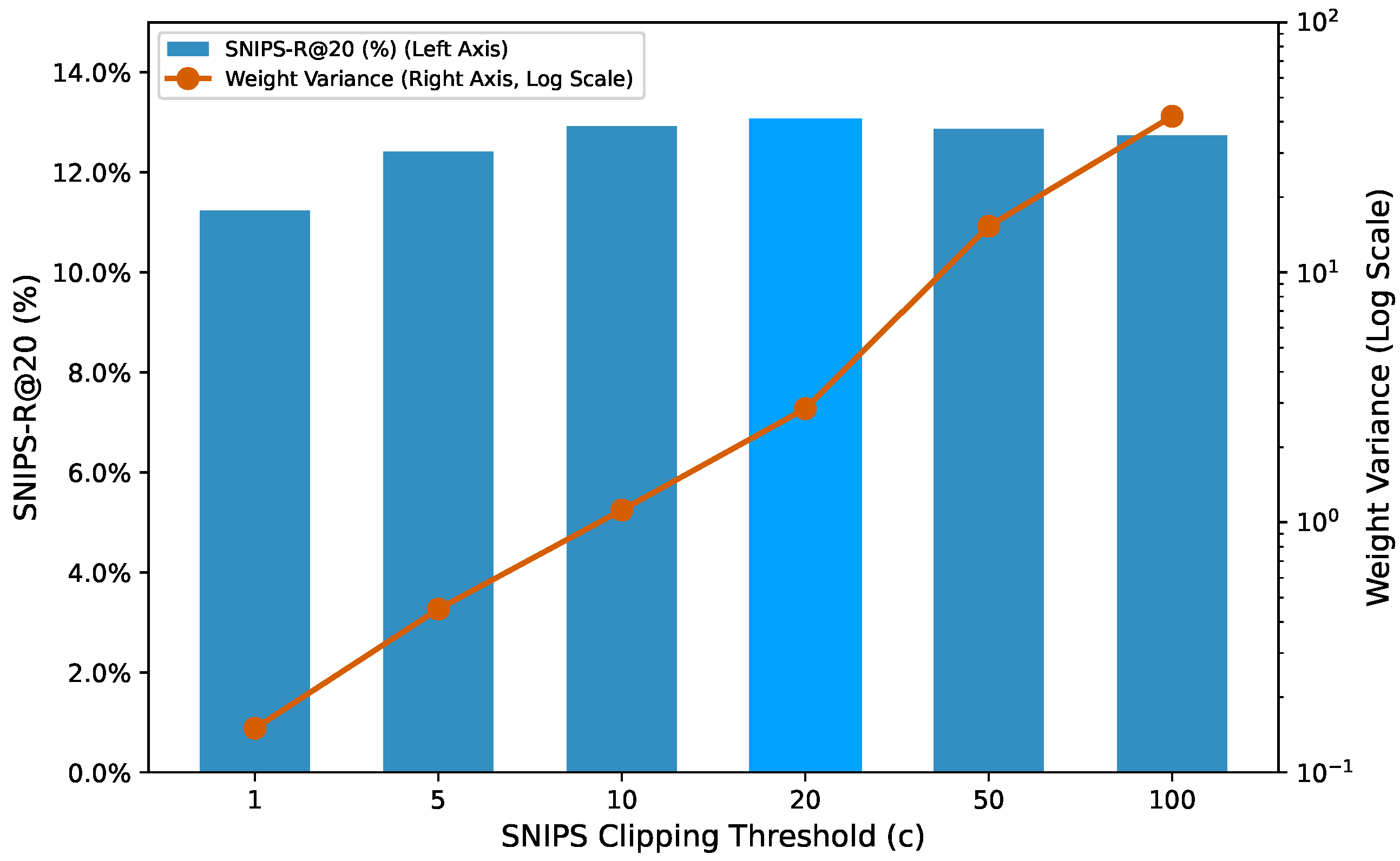
Figure 8.
Sensitivity to the SNIPS clipping threshold c on KuaiRand-27K. The bars (left axis) show SNIPS-R@20, peaking at . The line (right axis, log scale) shows the weight variance, which increases exponentially after the optimal point, illustrating the bias–variance trade-off.
Figure 8.
Sensitivity to the SNIPS clipping threshold c on KuaiRand-27K. The bars (left axis) show SNIPS-R@20, peaking at . The line (right axis, log scale) shows the weight variance, which increases exponentially after the optimal point, illustrating the bias–variance trade-off.
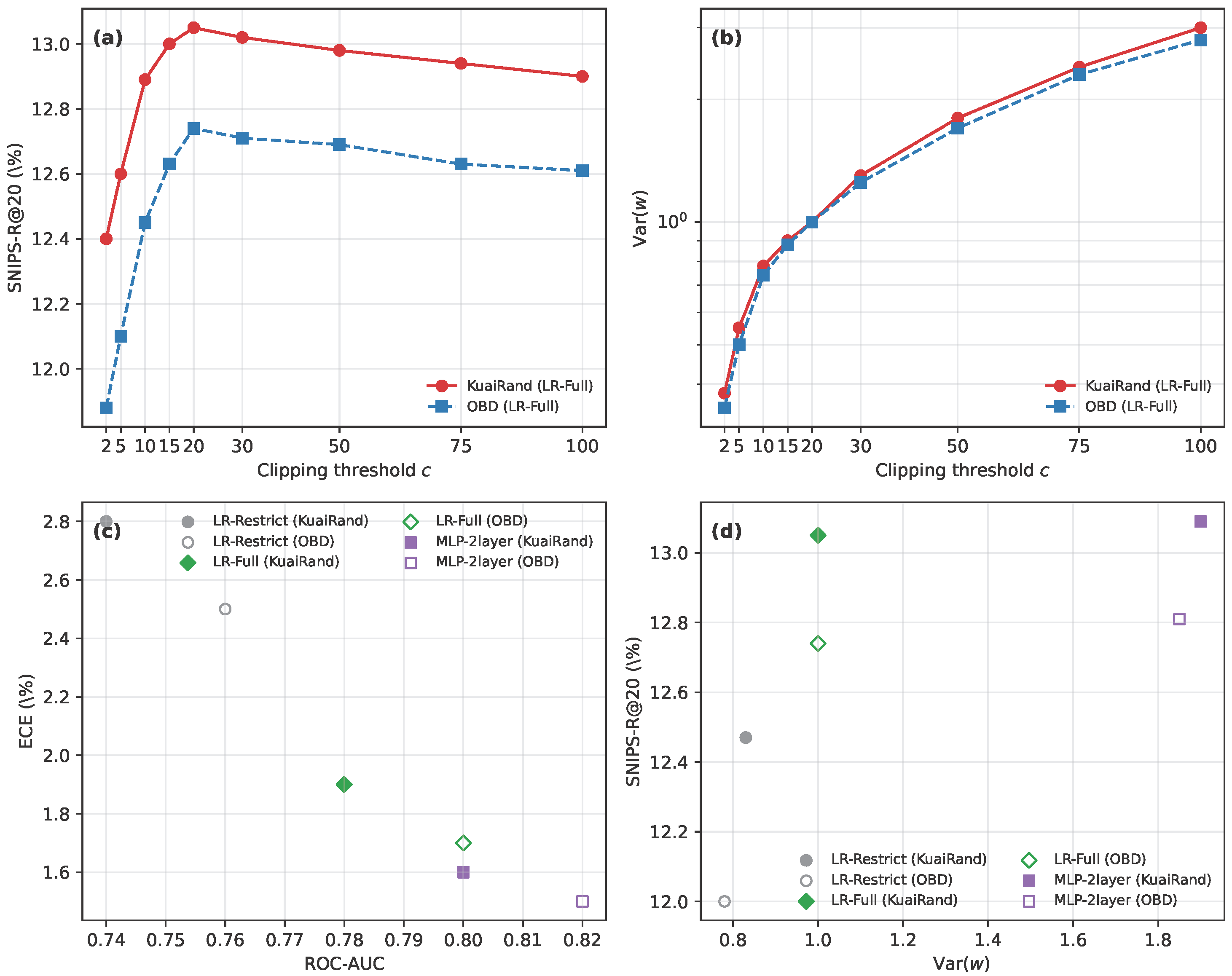
Figure 9.
Bias–variance and propensity model analysis on KuaiRand and OBD. Panel (a) shows SNIPS-R@20 as a function of the clipping threshold c for KuaiRand and OBD using the LR-Full propensity model. Panel (b) plots the corresponding variance of the SNIPS weights on a logarithmic scale. Panel (c) compares ROC-AUC versus ECE for three propensity models (LR-Restrict, LR-Full, MLP-2layer) on both datasets. Panel (d) shows SNIPS-R@20 versus Var.
Figure 10.
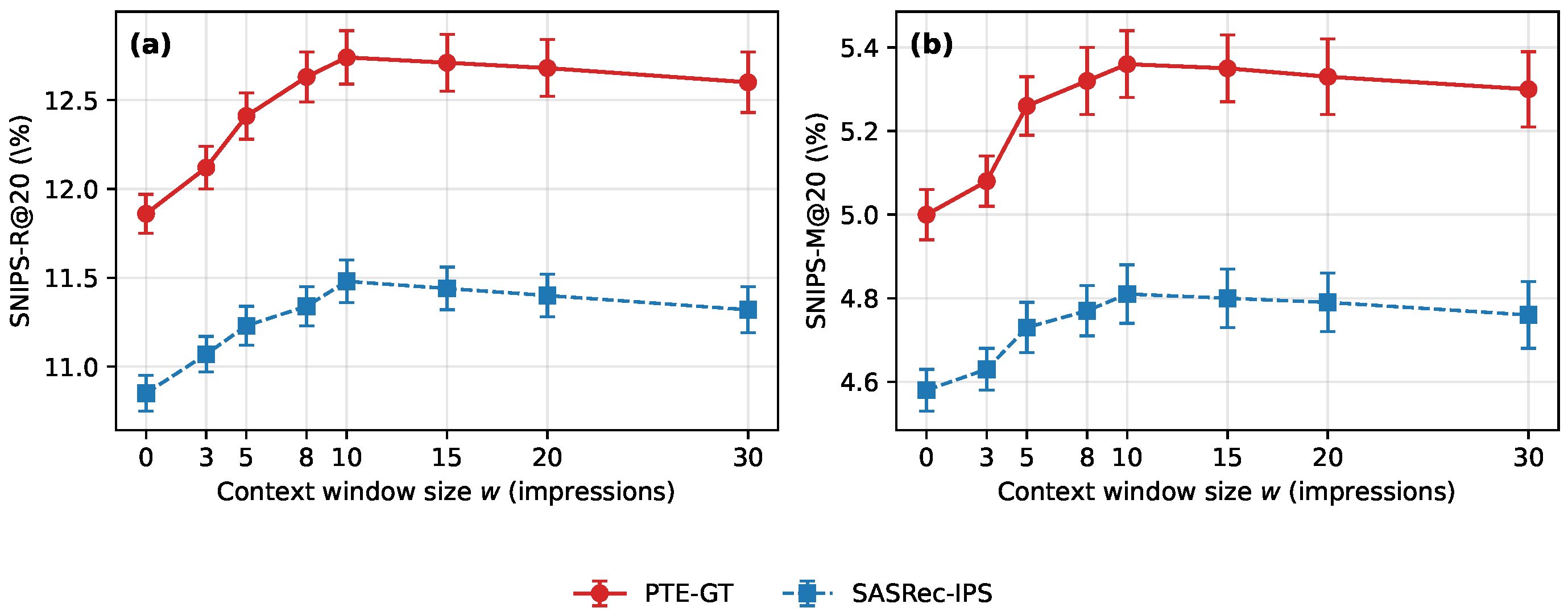
Effect of the context window size w on OBD. Panels (a,b) show SNIPS-R@20 and SNIPS-M@20, respectively, for PTE-GT and SASRec-IPS as w varies from 0 to 30 impressions. Points denote means over three random seeds and error bars denote one standard deviation.
Figure 10.
Effect of the context window size w on OBD. Panels (a,b) show SNIPS-R@20 and SNIPS-M@20, respectively, for PTE-GT and SASRec-IPS as w varies from 0 to 30 impressions. Points denote means over three random seeds and error bars denote one standard deviation.
Figure 11.
Qualitative analysis of the interval-aware attention mechanism. (a) Attention mass distribution over four structural edge types, revealing head specialization. (b) t-SNE projection of Fourier interval embeddings (). Colors show the dominant attention head, demonstrating a clear alignment between structural preference (a) and temporal preference (b).
Figure 12.
Case: Session flow Sankey with evidence weights. Evidence concentrates on time-salient shortcut edges (, ), forming dominant paths to the hit item L (P4: 30.2%, P1: 28.5%, P2: 26.6%), while the purely sequential path (P3: 14.7%) is comparatively weaker. This highlights non-sequential, structure-aware reasoning afforded by the graph transformer.
Table 1.
Dataset descriptive statistics. Note: OBD consists of impression-level bandit logs with logged propensities; session-length metrics are not directly applicable.
Table 1.
Dataset descriptive statistics. Note: OBD consists of impression-level bandit logs with logged propensities; session-length metrics are not directly applicable.
| Dataset (Split) | Sequence Unit | Sequences | Items | Interactions | Avg. Length | Randomized Propensities |
|---|
| KuaiRand-27K | user history | 27,285 | 32,038,725 | 322,278,385 | — | Yes |
| Open Bandit Dataset | impression log | 26 M | 80 | — | — | Yes (logged bandit) |
| OTTO (train) | session | 12,899,779 | 1,855,603 | 216,716,096 | 16.80 | No |
| YOOCHOOSE-1/64 | session | 369,859 | 16,766 | 557,248 | 6.16 | No |
Table 2.
Comparison of propensity models on KuaiRand and OBD. All SNIPS-R@20 and Var values use clipping threshold .
Table 2.
Comparison of propensity models on KuaiRand and OBD. All SNIPS-R@20 and Var values use clipping threshold .
| Dataset | Propensity Model | AUC | ECE (%) | Brier (%) | SNIPS-R@20 (%) | Var |
|---|
| KuaiRand | LR-Restrict | 0.74 | 2.80 | 7.50 | 12.47 | 0.83 |
| KuaiRand | LR-Full (ours) | 0.78 | 1.90 | 7.12 | 13.05 | 1.00 |
| KuaiRand | MLP-2layer | 0.80 | 1.60 | 7.05 | 13.09 | 1.90 |
| OBD | LR-Restrict | 0.76 | 2.50 | 6.50 | 12.00 | 0.78 |
| OBD | LR-Full (ours) | 0.80 | 1.70 | 6.20 | 12.74 | 1.00 |
| OBD | MLP-2layer | 0.82 | 1.50 | 6.15 | 12.81 | 1.85 |
Table 3.
Comprehensive performance and complexity comparison on OTTO and YOOCHOOSE-1/64 datasets (%). All results are averaged over five random seeds.
Table 3.
Comprehensive performance and complexity comparison on OTTO and YOOCHOOSE-1/64 datasets (%). All results are averaged over five random seeds.
| Model | Params (M) | OTTO (Clicks) | YOOCHOOSE-1/64 |
|---|
| R@10 | N@10 | M@10 | R@20 | N@20 | M@20 | R@10 | N@10 | M@10 | R@20 | N@20 | M@20 |
|---|
| Baselines (Reproduced/Literature) |
| GRU4Rec+ | 5.2 | 27.12 | 14.03 | 13.51 | 44.31 | 27.84 | 20.53 | 38.17 | 25.02 | 15.11 | 60.63 | 34.16 | 22.89 |
| SASRec | 6.8 | 19.04 | 11.52 | 11.03 | 30.71 | 20.13 | 18.02 | 45.91 | 32.14 | 19.06 | 69.17 | 40.82 | 29.88 |
| SR-GNN | 7.1 | 28.03 | 14.81 | 14.12 | 45.83 | 28.91 | 21.14 | 48.02 | 34.89 | 20.18 | 70.56 | 42.11 | 30.94 |
| TRON | 7.0 | 29.01 | 15.53 | 14.92 | 47.24 | 30.03 | 21.91 | 48.53 | 35.11 | 20.52 | 70.83 | 42.51 | 31.02 |
| Ours |
| IGT-Base | 7.5 | 29.54 | 15.92 | 15.21 | 47.91 | 30.52 | 22.34 | 48.71 | 35.26 | 20.61 | 70.97 | 42.63 | 31.07 |
| PTE-GT (Full) | 7.7 | 30.53 | 16.64 | 15.82 | 49.15 | 31.54 | 23.01 | 49.84 | 36.23 | 21.42 | 71.86 | 43.82 | 32.05 |
| Improv. (vs. TRON) | - | +5.24% | +7.15% | +6.03% | +4.04% | +5.03% | +5.02% | +2.70% | +3.19% | +4.39% | +1.45% | +3.08% | +3.32% |
Table 4.
Unbiased evaluation on KuaiRand and OBD (SNIPS-weighted, %). All metrics are averaged over five random seeds.
Table 4.
Unbiased evaluation on KuaiRand and OBD (SNIPS-weighted, %). All metrics are averaged over five random seeds.
| Model | KuaiRand-27K | OBD (All) |
|---|
| | SNIPS-R@20 (%) | SNIPS-M@20 (%) | SNIPS-R@20 (%) | SNIPS-M@20 (%) |
|---|
| SASRec | 10.15 | 4.32 | 9.92 | 4.18 |
| IGT-Base | 10.88 | 4.65 | 10.63 | 4.44 |
| SASRec-IPS | 11.75 | 5.02 | 11.48 | 4.87 |
| CausalRec-adapt | 12.03 | 5.21 | 11.96 | 5.04 |
| DR-JL | 12.54 | 5.32 | 12.31 | 5.17 |
| PTE-GT (Full Model) | 13.05 | 5.58 | 12.74 | 5.36 |
Table 5.
Calibration performance on OTTO and KuaiRand (ECE (%), Brier (%)).
Table 5.
Calibration performance on OTTO and KuaiRand (ECE (%), Brier (%)).
| Model | OTTO (Standard) | KuaiRand (Unbiased) |
|---|
| | ECE (%) | Brier (%) | ECE (%) | Brier (%) |
|---|
| IGT-Base | 5.12 | 7.82 | 6.45 | 9.18 |
| PTE-GT | 2.85 | 5.11 | 3.11 | 6.24 |
Table 6.
Ablation study of PTE-GT components. IGT-Base is our backbone, PA applies the SNIPS objective, and TC adds temporal consistency regularization.
Table 6.
Ablation study of PTE-GT components. IGT-Base is our backbone, PA applies the SNIPS objective, and TC adds temporal consistency regularization.
| Model Variant | KuaiRand-27K (Unbiased) | OTTO (Standard) |
|---|
| | SNIPS-R@20 (%) | ECE (%) | Long-Tail R@20 (%) | R@20 (%) | ECE (%) |
|---|
| (1) IGT-Base | 10.88 | 6.45 | 4.93 | 47.92 | 5.12 |
| (2) w/o PA (IGT-Base + TC) | 11.05 | 6.23 | 5.11 | 48.31 | 4.95 |
| (3) w/o TC (IGT-Base + PA) | 12.65 | 3.33 | 7.81 | 48.82 | 3.12 |
| (4) PTE-GT (Full Model) | 13.05 | 3.11 | 8.15 | 49.13 | 2.85 |
Table 7.
Statistical significance of PTE-GT compared to strong baselines (R@20 or SNIPS-R@20, five random seeds). Mean differences and confidence intervals are reported in percentage points (pp).
Table 7.
Statistical significance of PTE-GT compared to strong baselines (R@20 or SNIPS-R@20, five random seeds). Mean differences and confidence intervals are reported in percentage points (pp).
| Dataset | Metric | Comparison | Mean Diff (pp) | 95% CI (pp) | p-Value |
|---|
| OTTO | R@20 | PTE-GT vs. TRON | +1.91 | [+1.70, +2.10] | < |
| OTTO | R@20 | PTE-GT vs. IGT-Base | +1.24 | [+1.05, +1.43] | 0.0003 |
| YOOCHOOSE | R@20 | PTE-GT vs. SR-GNN | +1.30 | [+0.65, +1.95] | 0.002 |
| YOOCHOOSE | R@20 | PTE-GT vs. IGT-Base | +0.89 | [+0.05, +1.73] | 0.041 |
| KuaiRand | SNIPS-R@20 | PTE-GT vs. IGT-Base | +2.17 | [+1.96, +2.38] | < |
| OBD | SNIPS-R@20 | PTE-GT vs. SASRec-IPS | +1.26 | [+0.72, +1.80] | 0.001 |
| OBD | SNIPS-R@20 | PTE-GT vs. DR-JL | +0.64 | [+0.15, +1.13] | 0.033 |
