Image Haze Removal Using Dual Dark Channels with the Whale Optimization Algorithm and an Image Regression Model

Abstract

Recently, image haze removal has gained increasing attention in the field of image restoration. Data-driven and model-based methods are popular among researchers. The dark channel prior prevails in model-based methods, where the model parameters, atmospheric light, and transmittance are generally estimated through a block-based dark channel. This paper proposes a model-based approach with integrated pixel- and block-based dark channels for initial transmittance estimation. Additionally, we developed a two-stage guided image filtering process to refine the initial transmittance while utilizing the pixel-based dark channel to estimate atmospheric light. Our approach introduces two scaling factors for atmospheric light and initial transmittance, which are optimized using the Whale Optimization Algorithm. A CNN image regression model is employed to learn the mapping between hazy images and their corresponding optimized scaling factors, thus eliminating the need for ground-truth images. This makes our approach applicable in real-world scenarios. The proposed approach was validated using two datasets: an artificially generated image dataset, RESIDE, and a natural image dataset, KeDeMa. The results show that our approach outperforms four other dehazing methods, i.e., GCAN, RRO, RFDN, and Ka-Net. With the RESIDE dataset, our approach outperforms GCAN, RRO, RFD, and Ka-Net by 2.009 dB, 6.042 dB, 3.488 dB, and 8.975 dB, respectively, in terms of PSNR. With the KeDeMa dataset, our approach generally demonstrates superior visual quality to the four comparison methods. The results suggest that the proposed model-based approach may outperform data-driven methods.

1. Introduction

Image dehazing or haze removal has recently received increasing attention in image restoration. Haze is mainly caused by the scattering of suspended particles in the air. Hazy images often have lower contrast and visibility, which degrades the performance of subsequent image-based systems, such as object tracking and surveillance systems. Thus, image dehazing methods have been sought to solve the problem. Besides conventional image processing techniques like histogram equalization and contrast enhancement, image dehazing methods can be roughly categorized into three types: network-based, model-based, and hybrid (network–model-based) methods. Network-based methods are associated with end-to-end deep learning models, which are irrelevant to this study. They will not be discussed further. Model-based methods are based on a haze image model. Its challenge is to appropriately estimate model parameters, i.e., atmospheric light and transmittance. Hybrid models generally use networks to extract model parameters and integrate them into the training process. For a comprehensive survey, one may consult [1,2,3].

Regarding model-based dehazing methods, a widely used image haze model is expressed as follows [4]:

$$I\left(x\right)=J\left(x\right)t\left(x\right)+A[1-t(x)]$$

(1)

where $I\left(x\right)$ refers to the observed intensity; $x$ is the pixel coordinate; $J\left(x\right)$ is the radiance of the captured image; $A$ is the atmospheric light; and $t(x)=e^{-\rho d(x)}$ describes the transmittance of un-scattered light to a camera, where $\rho$ is the scattering coefficient, and $d(x)$ is the depth at $x$. The challenge with model-based methods lies in accurately estimating the model parameters $A$ and $t(x)$ in Equation (1).

To estimate model parameters in Equation (1), researchers have developed methods based on various assumptions and statistical priors. A single-image dehazing method that assumes the transmittance and surface shading are locally uncorrelated was introduced in [5]. In [6], color lines were introduced in the dehazing process. The color lines refer to a characteristic found in natural images, where pixels in small patches create one-dimensional distributions within the RGB color space. A color attenuation prior was proposed in [7] that enables the estimation of scene depth in hazy images using a linear model with supervised learning. The depth map was then used to estimate the transmittance. In [8], a convolutional neural network was proposed to estimate transmittance in a hazy image. Then, the dehazed image was obtained based on the image haze model. A dark channel prior (DCP) was introduced in [9] to estimate model parameters $A$ and $t(x)$. The DCP prevails in the field of image dehazing due to its simplicity. However, it is known that the DCP suffers from artifacts, halo effects, color distortion, and high computational costs. Many researchers have consequently proposed approaches to improve its performance. In [10], atmospheric light was estimated using dark channels and a decision image. A multi-scale retinex with a color restoration algorithm was proposed to estimate initial transmittance, which was then optimized to obtain the final transmittance. A modified DCP was proposed in [11], where scaling factors for atmospheric light and initial transmittance were introduced to enhance the performance of the DCP. In [12], a combined optimization method for radiance and reflectance was applied to estimate transmittance. A transmittance estimation scheme was proposed in [13], where a lower bound and a nonlinear bounding function were used. An approach using robust sky detection was proposed in [14] to eliminate the halos that occur in sky regions. In [15], a sky region segmentation method based on particle swarm optimization and the Otsu segmentation scheme was presented. The final dark channel was formed by a compensated dark channel in the sky regions and the dark channel in the non-sky regions. A convolutional neural network called the All-in-One Dehazing Network (AOD-Net) was proposed in [16]. In this method, the image haze model is reformulated to adapt to the end-to-end learning process. In [17], an improved AOD-Net was reported, where a depth-separable convolutional neural network was introduced to obtain the optimal model parameters. A support vector regression model was employed in [18] to learn transmittance from image patches and estimate patch transmittances during the dehazing process. Atmospheric light was estimated through median and maximum filters. Both model parameters were then refined using guided image filtering. In [19], an unsupervised deep learning approach to image dehazing was proposed, through which the dark channel prior energy function was minimized. In [20], a hybrid learning method for image haze removal that used a patch map and a bi-attentive generative adversarial network was proposed. The former adaptively selected patch sizes for dark channel calculation, and the latter was a pre-trained network that estimated parameters for the adaptive patch map. A generative adversarial network was introduced to optimize model parameters in [21]. In [22], a hybrid approach to image dehazing was proposed. Atmospheric light and transmittance were estimated using deep learning schemes to balance the computational cost and dehazing performance. An efficient dehazing method that uses the pixel-based dark channel and the pixel-based bright channel was presented in [23]. The atmospheric light was estimated according to haze density analysis. In [24], a fusion-based method was proposed that employed both pixel-based and patch-based dark channels, which were smoothed using $l_0$ filtering and Gaussian filtering, respectively. The final transmittance was obtained by fusing both dark channels with an adaptive lower bound threshold. In our previous study [25], a pixel-based dark channel was applied to estimate atmospheric light and initial transmittance. In addition, adaptive scaling factors were introduced for the two model parameters. The pixel-based dark channel was also used in guided image filtering as a guidance image. In [26], a multi-scale fusion method was proposed for transmittance estimation. The method fused weighted dark channels at different scales and a bright channel to estimate transmittance. A quad-tree-based method was employed in [27] to estimate atmospheric light, while a linear regression model was used to determine the scattering coefficient of transmittance based on features of mean brightness and mean saturation. In [28], a modified atmospheric scattering model was proposed, along with a corresponding image clarification algorithm designed to enhance robustness and mitigate color distortion in hazy images. The method segmented the image into dense haze and non-dense haze regions. The atmospheric light and transmittance were estimated separately in segmented regions. Then, an alpha fusion was used to obtain the final estimates. An image dehazing algorithm based on an improved atmospheric scattering model was introduced in [29] to address issues of low visibility, poor contrast, color distortion, and image darkening caused by haze. The proposed model improved the traditional atmospheric scattering model by introducing a light absorption coefficient to prevent darkening. The equation for the transmittance map was then mathematically fitted and transformed into a simple quadratic equation to improve efficiency. The model-based methods mentioned above either modify the image haze model or incorporate optimization algorithms, deep learning schemes, and regression models. In this study, a model-based approach is proposed based on dual dark channels (DDCs), two-stage transmittance refinement, and a convolutional neural network (CNN) image regression. Our method is fundamentally different from the abovementioned methods.

Regarding hybrid methods, an image dehazing algorithm was proposed in [30]. This algorithm features a reformulated compensation atmospheric scattering model to improve performance in real-world scenes by compensating for modeling errors and inaccurate parameter estimation. In addition, a lightweight two-branch network was employed to jointly estimate the transformation map and the compensation map. In [31], an end-to-end asymmetric U-Net dehazing network was proposed, driven by an atmospheric scattering model with a two-stage process. A simplified U-Net was used to estimate the atmospheric light, while an asymmetric U-Net guided by the dark channel prior was employed to estimate the transmittance. An attention module was also employed to enhance performance. A physics-aware dehazing network using a seven-stage U-Net variant was proposed in [32]. This method relied on a derived haze extraction model that combines residual learning with the atmospheric scattering model. An atmospheric scattering prior embedded diffusion model was introduced in [33]. This model integrates atmospheric physics into the diffusion-based generative restoration process. An atmospheric prior estimation module is utilized to refine the initial transmittance, while learnable networks are used to estimate atmospheric light from the dark channel prior and physical consistency loss. In [34], a remote sensing image dehazing method was presented that integrates an atmospheric scattering model and a dark-channel prior-constrained network. The method is composed of three interconnected networks: a dehazing network, a transmittance network, and a dark channel information injection network. Traditional loss functions and a dark channel loss function were used to obtain a dehazed image. A two-stage framework for image dehazing was introduced in [35]. The method combined a physics-based dehazing network with a contrastive learning-based generative adversarial network. The former network was trained with synthetic image pairs in the first stage, while the latter network was used to bridge the domain gap between synthetic and real data.

Although a CNN image regression model was used in the study, the proposed approach differs from the hybrid methods described above and is essentially a model-based method. Our method solely relies on the image haze model. The model parameters for hazy images are used as the outputs to train a CNN image regression model, rather than the hazy image itself. The proposed approach consists of three parts. First, a dehazing scheme based on pixel- and block-based dark channels was developed, utilizing adaptive scaling factors for atmospheric light and initial transmittance. The dehazing scheme is called DDC. Second, the Whale Optimization Algorithm (WOA) [36] with a full-reference image quality assessment (FRIQA) was introduced to find optimal scaling factors in the DDC. The scheme is called the DDC_WOA. The objective of the DDC_WOA is to find pairs of input hazy images and their optimal scaling factors within an image dataset, such as RESIDE [37]. Third, with the pairs identified by the DDC_WOA, a CNN image regression model was employed to learn the mapping between pairs, thus eliminating the need for ground-truth (GT) images in the WOA. This makes our approach applicable in real-world applications. The proposed dehazing approach is referred to as DDC_WOA_CNN. In the application of the DDC_WOA_CNN method, the trained CNN estimates the corresponding optimal scaling factors for an input hazy image, which are then used in the DDC to obtain a dehazed image. In the experiment, we used the artificially generated hazy image dataset RESIDE [37] and the natural hazy image dataset KeDeMa [38] to verify the proposed DDC_WOA_CNN approach and compare it with four other dehazing methods, i.e., the GCAN [39], RRO [12], RFDN [40], and Ka-Net [41]. The results show that the DDC_WOA_CNN method has a higher PSNR in the RESIDE dataset than the GCAN, RRO, RFDN, and Ka-Net by 2.009 dB, 6.042 dB, 3.488 dB, and 8.975 dB, respectively. In the KeDeMa dataset, the subjective visual quality of the DDC_WOA_CNN method is generally better than that of the comparison methods. This paper has at least three contributions, as listed below.

• We developed an image haze removal method called DDC based on pixel- and block-based dark channels and derived a scheme to estimate the initial transmittance in the DDC. Then, we introduced two-stage transmittance refinement, i.e., the coarse and smooth refinements, where two different guided image filters were applied. This is the first attempt of its kind in the field.
• We applied the WOA to find optimal scaling factors for atmospheric light and initial transmittance in the DDC. The DDC with optimized scaling factors is referred to as the DDC_WOA. The DDC_WOA offers an alternative scheme to applying optimization algorithms in model-based methods. It is different from the models of most researchers, who have attempted to directly optimize atmospheric light and/or transmittance.
• We introduced a CNN image regression model to learn the mapping between hazy images and their corresponding scaling factors obtained by the DDC_WOA. This eliminates the requirement for GT images in FRIQA and enables the use of the model in real-world applications. The resulting method is called DDC_WOA_CNN. The novelty of the proposed DDC_WOA_CNN method is demonstrated in the integration of the WOA and CNN into the model-based dehazing method DDC.

This paper is organized as follows: Section 2 describes the development of our DDC dehazing method. Section 3 introduces the proposed DDC_WOA_CNN method. Section 4 justifies the proposed approach. Finally, Section 5 concludes this study.

2. Our DDC Dehazing Method

In this section, we briefly review the DCP [9] in Section 2.1. Then, Section 2.2 describes the development of our DDC dehazing method.

2.1. The DCP Dehazing Method

In the DCP, the image haze model in Equation (1) is assumed. The DCP is based on a statistical observation that pixels in a non-sky patch of outdoor haze-free images generally have zero or very low pixel values in at least one of the RGB components. This statistical property is called the dark channel prior. A dark channel can be obtained using a block-based minimum filter. The model parameters in Equation (1) can be easily estimated through the dark channel. The DCP is popular in the image dehazing community due to its simplicity. For more details, see [9]. Given an RGB image I, the implementation of the DCP is summarized below.

Step 1.

Find the dark channel using a $N\times N$ minimum filter as

$$I_{\mathsf{\Omega }}^{dark}\left(x\right)=\underset{y\in \mathsf{\Omega }\left(x\right)}{\min }\underset{c}{\min }\left[I_c\left(y\right)\right]$$

(2)

where $\mathsf{\Omega }\left(x\right)$ is a $N\times N$ window centered at $x$ and $c\in \{R,G,B\}$. In [9], $N=15$.

Step 2.

Find the 0.1% pixels with the highest values in $I_{\mathsf{\Omega }}^{dark}\left(x\right)$. Then, trace back to the corresponding pixels in the image $\mathit{I}$ and find the pixel with the highest intensity, ${\mathit{p}}_{max}$.

Step 3.

Estimate the atmospheric light $\mathit{A}=[A_R A_G A_B]$ as $\alpha \times {\mathit{p}}_{max}$, where $\alpha$ is a scaling factor. In [9], $\alpha =1$.

Step 4.

Calculate the normalized dark channel as

$${\overline{I}}_{\mathsf{\Omega }}^{dark}(x)=\underset{y\in \mathsf{\Omega }\left(x\right)}{\min }\underset{c}{\min }\left[{\displaystyle \frac{I_c\left(y\right)}{A_c}}\right]$$

(3)

Step 5.

Obtain the initial transmittance as

$$\tilde{t}\left(x\right)=1-\omega \times {\overline{I}}_{\mathsf{\Omega }}^{dark}(x)$$

(4)

where $0<\omega <1$ is a user-defined scaling factor. In [9], $\omega =0.95$.

Step 6.

Refine the initial transmittance $\tilde{t}\left(x\right)$ using the soft matting algorithm [9] or the guided image filter (GIF) in [42] to obtain the final transmittance $t\left(x\right)$. The settings for the GIF are as follows: input image $\mathit{I}$ is the guidance image; window size $W=20$; and smoothing factor $ϵ=0.001$.

Step 7.

Recover the scene radiance as

$${\widehat{J}}_c\left(x\right)={\displaystyle \frac{I_c\left(x\right)-A_c}{\max \left[t_{0,}t\left(x\right)\right]}}+A_c$$

(5)

where $t_0$ is a user-defined lower bound of $t\left(x\right)$. In [9], $t_0=0.1$.

2.2. The Proposed DDC Dehazing Method

This section describes the proposed DDC and its implementation. Section 2.2.1 and Section 2.2.2 describe the estimation of atmospheric light $\mathit{A}$ and transmittance $t(x)$ in the DDC. The overall algorithm of the DDC is given in Section 2.2.3.

2.2.1. Estimation of Atmospheric Light

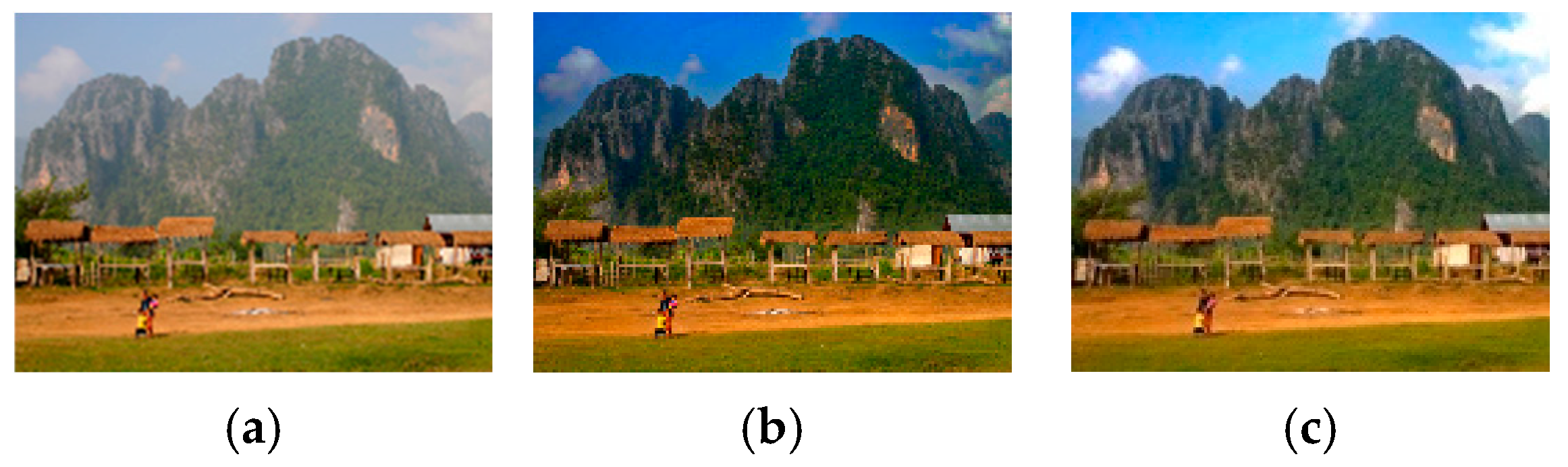
Hue distortion is often found in dehazed images in the DCP. As proven in [43], this distortion results from estimation error in atmospheric light $\mathit{A}$. In other words, inappropriate estimation of $\mathit{A}$ leads to hue distortion in the DCP. As described in our previous work [44], an adaptive scaling factor can alleviate this problem. For example, consider the hazy village image shown in Figure 1a. Figure 1b shows the DCP result with a scaling factor $\alpha =1$ for $\mathit{A}$, while Figure 1c shows the result with $\alpha =0.85$. The result shows that hue distortion is found in the sky regions in Figure 1b, whereas the distortion is not present in Figure 1c with $\alpha =0.85$. This suggests that using an appropriate scaling factor can help the estimation of $\mathit{A}$. In this study, we used an adaptive scaling factor ${\alpha }_a$ for $\mathit{A}$ in the DDC and applied the WOA [36] to find the optimal scaling factor ${\alpha }^{\mathrm{*}}$ for $\mathit{A}$ in the DDC_WOA. The details will be given in Section 3.

2.2.2. Estimation of Transmittance

In this study, the transmittance estimation was motivated by two observations on the pixel-based dark channel (PDC) and block-based dark channel (BDC). The dual dark channels were utilized in estimating the initial transmittance. The transmittance derived from the PDC tends to preserve edges and details within objects better than that derived from the BDC. However, it may introduce color distortion. On the other hand, the transmittance obtained from the BDC has superior dark channel prior properties compared to the PDC, but it may lose object details. We attempted to integrate both advantages in estimating initial transmittance in this study. Moreover, transmittance refinement using a single GIF is found to be both efficient and effective in most cases, as shown in [42]. However, a single GIF may suffer from the halo problem when significant depth discontinuities are present. The situation becomes even worse when dual dark channels are considered. To address this challenge, we propose transmittance refinement based on a two-stage GIF scheme. The details are described below.

Next, a mathematical expression is derived for the initial transmittance estimation (ITE) using dual dark channels (DDCs), i.e., the PDC and the BDC. This scheme is called ITE/DDCs. The differences between ITE/DDCs and those used in the DCP are also explained.

Given that an RGB image $\mathit{I}$ does not contain any sky regions or white objects, the dark channel prior suggests that at least one of the RGB components typically has very low intensity in patches of the image. The dark channel can be obtained through minimum filtering. When a 1 × 1 minimum filter is used, it is called the PDC, while using a block-based minimum filter, such as 15 × 15 in the DCP, is called the BDC. Using Equation (1), we can derive the initial transmittance $\tilde{t}(x)$ based on DDCs, i.e., the PDC and the BDC.

By normalizing with $A_c$ and applying a pixel-wise minimum operation over RGB components on both sides of Equation (1), we obtain the normalized PDC as

$$\underset{c}{\min }\left[{\displaystyle \frac{I_c\left(x\right)}{A_c}}\right]=\tilde{t}(x)\underset{c}{\min }\left[{\displaystyle \frac{J_c\left(x\right)}{A_c}}\right]+1-\tilde{t}(x)$$

(6)

Similarly, by normalizing with $A_c$ and applying a block minimum operation over RGB channels on both sides of Equation (1), we obtain the normalized BDC as

$$\underset{y\in \mathsf{\Omega }\left(x\right)}{\min }\underset{c}{\min }\left[{\displaystyle \frac{I_c\left(y\right)}{A_c}}\right]=\tilde{t}\left(x\right)\underset{y\in \mathsf{\Omega }\left(x\right)}{\min }\underset{c}{\min }\left[{\displaystyle \frac{J_c\left(y\right)}{A_c}}\right]+1-\tilde{t}(x)$$

(7)

where $\mathsf{\Omega }\left(x\right)$ is a square patch of $\mathit{I}$ centered at $x$. By subtracting Equation (7) from Equation (6), we have

$$\underset{c}{\min }\left[{\displaystyle \frac{I_c\left(x\right)}{A_c}}\right]-I_{\mathsf{\Omega }}^{dark}\left(x\right)=\tilde{t}\left(x\right)\left\{\underset{c}{\min }\left[{\displaystyle \frac{J_c\left(x\right)}{A_c}}\right]-J_{\mathsf{\Omega }}^{dark}\left(x\right)\right\}$$

(8)

where $J_{\mathsf{\Omega }}^{dark}\left(x\right)=\underset{y\in \mathsf{\Omega }\left(x\right)}{\min }\underset{c}{\min }\left[{\displaystyle \frac{J_c\left(x\right)}{A_c}}\right]$. According to the property of the dark channel prior, $J_{\mathsf{\Omega }}^{dark}\left(x\right)\to 0$. Thus, Equation (8) can be written as

$$\underset{c}{\min }\left[{\displaystyle \frac{I_c\left(x\right)}{A_c}}\right]-I_{\mathsf{\Omega }}^{dark}(x)=\tilde{t}\left(x\right)\underset{c}{\min }\left[{\displaystyle \frac{J_c\left(x\right)}{A_c}}\right]$$

(9)

To estimate the initial transmittance, Equation (9) is rearranged as

$$\tilde{t}\left(x\right)={\displaystyle \frac{I_1^{dark}\left(x\right)-I_{\mathsf{\Omega }}^{dark}(x)}{J_1^{dark}(x)}}$$

(10)

where $I_1^{dark}\left(x\right)=\underset{c}{\min }\left[{\displaystyle \frac{I_c\left(x\right)}{A_c}}\right]$ and $J_1^{dark}\left(x\right)=\underset{c}{\min }\left[{\displaystyle \frac{J_c\left(x\right)}{A_c}}\right]$.

For a haze-free image $\mathit{I}$, $I_1^{dark}\left(x\right)=J_1^{dark}\left(x\right)$, and $I_{\mathsf{\Omega }}^{dark}\left(x\right)=J_{\mathsf{\Omega }}^{dark}(x)$. Thus, Equation (10) can be rewritten as

$$\tilde{t}\left(x\right)={\displaystyle \frac{I_1^{dark}\left(x\right)-I_{\mathsf{\Omega }}^{dark}(x)}{J_1^{dark}(x)}}=1-{\displaystyle \frac{J_{\mathsf{\Omega }}^{dark}\left(x\right)}{J_1^{dark}\left(x\right)}}=1$$

(11)

In this case, $\tilde{t}\left(x\right)=t\left(x\right)=1$ in Equation (1). In other words, $\mathit{I}$ is identical to the haze-free image $\mathit{J}$.

For a hazy image, Equation (10) can be rewritten as

$$\tilde{t}\left(x\right)={\displaystyle \frac{I_1^{dark}\left(x\right)-I_{\mathsf{\Omega }}^{dark}\left(x\right)}{J_1^{dark}\left(x\right)}}={\displaystyle \frac{I_1^{dark}\left(x\right)}{J_1^{dark}\left(x\right)}}\left[1-{\displaystyle \frac{I_{\mathsf{\Omega }}^{dark}\left(x\right)}{I_1^{dark}\left(x\right)}}\right]=w(x)\left[1-{\displaystyle \frac{I_{\mathsf{\Omega }}^{dark}\left(x\right)}{I_1^{dark}\left(x\right)}}\right]$$

(12)

where $w(x)=I_1^{dark}\left(x\right)/J_1^{dark}\left(x\right)$. For a hazy image, $I_1^{dark}(x)\ge J_1^{dark}(x)$ because of the haze in the image $\mathit{I}$. By applying the inequality, Equation (12) can be rewritten as follows:

$$\begin{array}{l}\tilde{t}\left(x\right)={\displaystyle \frac{I_1^{dark}\left(x\right)}{J_1^{dark}\left(x\right)}}\left[1-{\displaystyle \frac{I_{\mathsf{\Omega }}^{dark}\left(x\right)}{I_1^{dark}\left(x\right)}}\right]\\ \hspace{1em} ={\displaystyle \frac{J_1^{dark}\left(x\right)+{∆I}_1^{dark}\left(x\right)}{J_1^{dark}\left(x\right)}}\left[1-{\displaystyle \frac{I_{\mathsf{\Omega }}^{dark}\left(x\right)}{I_1^{dark}\left(x\right)}}\right]\\ \hspace{1em} =\left[1+{\displaystyle \frac{{∆I}_1^{dark}\left(x\right)}{J_1^{dark}\left(x\right)}}\right]\left[1-{\displaystyle \frac{I_{\mathsf{\Omega }}^{dark}\left(x\right)}{I_1^{dark}\left(x\right)}}\right]\\ \hspace{1em} =w(x)\left[1-{\displaystyle \frac{I_{\mathsf{\Omega }}^{dark}\left(x\right)}{I_1^{dark}\left(x\right)}}\right]\end{array}$$

(13)

where ${∆I}_1^{dark}\left(x\right)=I_1^{dark}\left(x\right)-J_1^{dark}\left(x\right)$ is related to the haze level in $\mathit{I}$, and $w\left(x\right)={\displaystyle \frac{I_1^{dark}\left(x\right)}{J_1^{dark}\left(x\right)}}=1+{\displaystyle \frac{{∆I}_1^{dark}\left(x\right)}{J_1^{dark}\left(x\right)}}$.

The initial transmittance estimation in ITE/DDCs differs from that in the DCP at least in two main aspects. First, the DCP uses only the BDC to obtain the initial transmittance $\tilde{t}\left(x\right)$ as in Equation (4). In contrast, the proposed ITE/DDC method uses both the PDC $I_1^{dark}\left(x\right)$ and the BDC $I_{\mathsf{\Omega }}^{dark}\left(x\right)$ as in Equation (12). Second, while the DCP uses a fixed weight $\omega$ for all pixels as in Equation (4), ITE/DDCs uses a coordinate-dependent weight $w(x)$ for each pixel. These differences contribute to the superior performance of ITE/DDCs compared to the DCP. This will be verified later in this study.

Note that $w(x)$ uses $J_1^{dark}\left(x\right)$ in Equation (13). However, $J_1^{dark}\left(x\right)$ is not available in real-world applications. Therefore, we need a way to estimate $w(x)$. A scheme based on the following two observations was developed: (i) $w(x)$ in Equation (13) includes the term ${∆I}_1^{dark}\left(x\right)=I_1^{dark}\left(x\right)-J_1^{dark}\left(x\right)$, which is related to the haze level in $\mathit{I}$, and (ii) the PDC $I_1^{dark}(x)$ is proportional to the haze level in $\mathit{I}$. In other words, $w(x)$ in Equation (13) can be estimated as $w(x){=\beta [1+I}_1^{dark}\left(x\right)]$, where $\beta$ is a scaling factor. Accordingly, the initial transmittance in Equation (13) is estimated as follows:

$$\tilde{t}\left(x\right)={\beta [1+I}_1^{dark}\left(x\right)]\left[1-{\displaystyle \frac{I_{\mathsf{\Omega }}^{dark}\left(x\right)}{I_1^{dark}\left(x\right)}}\right],$$

(14)

In this study, we propose a two-stage GIF (TSGIF) scheme to refine the initial transmittance $\tilde{t}\left(x\right)$ obtained from ITE/DDCs. The TSGIF refinement processes edges and details separately, which consists of two parts: rough refinement and smooth refinement. The rough refinement utilizes a GIF to preserve edges and eliminate halos, while the smooth refinement employs another GIF to detail smoothness to improve transmittance estimation.

We have shown how the model parameters $\mathit{A}$ and $t\left(x\right)$ are estimated in the proposed DDC. The implementation of the DDC is given in the next section.

2.2.3. Implementation of the Proposed DDC

This section summarizes the proposed DDC with implementation steps. Given an RGB image $\mathit{I}$, the implementation of the DDC is described below.

Step 1.

Find the initial block-based dark channel using a $N\times N$ minimum filter as

$${\tilde{I}}_{\mathsf{\Omega }}^{dark}(x)=\underset{y\in \mathsf{\Omega }\left(x\right)}{\min }\underset{c}{\min }\left[I_c\left(y\right)\right]$$

(15)

where $\mathsf{\Omega }\left(x\right)$ is a $N\times N$ window centered at $x$ and $c\in \{R,G,B\}$. In the following experiment, $N=15$.

Step 2.

Find the 0.1% pixels with the highest values in ${\tilde{I}}_{\mathsf{\Omega }}^{dark}(x)$. Then, trace back to the corresponding pixels in $\mathit{I}$, and find the pixel with the highest intensity, ${\mathit{p}}_{max}$.

Step 3.

Estimate the atmospheric light $\mathit{A}=[A_R A_G A_B]$ as ${{\alpha }_a\times \mathit{p}}_{max}$, where the adaptive scaling factor ${\alpha }_a=\mathrm{m}\mathrm{i}\mathrm{n}\left\{{{(\mu }_{BDC})}^{0.075},0.975\right\}$ and ${\mu }_{BDC}=\mathrm{m}\mathrm{e}\mathrm{a}\mathrm{n}\left[{\tilde{I}}_{\mathsf{\Omega }}^{dark}\left(x\right)\right]$.

Step 4.

Calculate the normalized PDC as

$$I_1^{dark}\left(x\right)=\underset{c}{\min }\left[{\displaystyle \frac{I_c\left(x\right)}{A_c}}\right]$$

(16)

where $x$ is the pixel coordinate.

Step 5.

Find the pixel-based transmittance as

$${\tilde{t}}_1\left(x\right)=1-I_1^{dark}\left(x\right)$$

(17)

Step 6.

Calculate the normalized BDC as

$$I_{\mathsf{\Omega }}^{dark}(x)=\underset{y\in \mathsf{\Omega }\left(x\right)}{\min }\underset{c}{\min }\left[{\displaystyle \frac{I_c\left(y\right)}{A_c}}\right]$$

(18)

where $\mathsf{\Omega }\left(x\right)$ is an $N\times N$ window centered at $x$.

Step 7.

Find the initial transmittance as

$$\tilde{t}\left(x\right)=w(x)\times \left[1-{\displaystyle \frac{I_{\mathsf{\Omega }}^{dark}\left(x\right)}{I_1^{dark}\left(x\right)}}\right]$$

(19)

where ${w\left(x\right)={\beta }_a[1+I}_1^{dark}\left(x\right)]$ and the adaptive scaling factor ${\beta }_a=\mathrm{m}\mathrm{i}\mathrm{n}\left\{{\left({\mu }_{BDC}^{0.8}\right.)}^{0.45},0.95\right\}$ and ${\mu }_{BDC}^{0.8}=\mathrm{m}\mathrm{e}\mathrm{a}\mathrm{n}\left({\mu }_{BDC}\le 0.8\right)$.

Step 8.

Refine the initial transmittance $\tilde{t}\left(x\right)$ by rough refinement as

$${\tilde{t}}_r\left(x\right)={GIF}_r\left\{\tilde{t}\left(x\right),{\mathit{I}}_{gr},N_r,{ϵ}_r\right\}$$

(20)

where ${GIF}_r(·)$ is a 2-D GIF in [45]; ${\mathit{I}}_{gr}$ is the guidance image; $N_r$ is the window size; and ${ϵ}_r$ is the smoothing factor.

Step 9.

Obtain the final transmittance $t\left(x\right)$ by smooth refinement as

$$t\left(x\right)={GIF}_s\left\{{\tilde{t}}_r\left(x\right),{\mathit{I}}_{gs},N_s,{ϵ}_s\right\}$$

(21)

where ${GIF}_s(·)$ is the GIF in [43]; ${\mathit{I}}_{gs}$ is the guidance image; $N_s$ is the window size; and ${ϵ}_s$ is the smoothing factor.

Step 10.

Recover the scene radiance using Equation (5) as below

$${\widehat{J}}_c\left(x\right)={\displaystyle \frac{I_c\left(x\right)-A_c}{\max \left[t_{0,}t\left(x\right)\right]}}+A_c$$

where $t_0$ is a user-defined lower bound for $t\left(x\right)$ and is set to 0.1.

There are three points that should be mentioned regarding the proposed DDC. First, in Step 3, the scaling factor ${\alpha }_a$ for $\mathit{A}$ is determined via a gamma correction ${y=x}^{\gamma }$. It is based on the following three observations: (i) a smaller $\mathit{A}$ results in a brighter dehazed image and vice versa. According to our experiments, the dehazed image from a less hazy image exhibits better visual quality. That is, a small $\mathit{A}$ is appropriate for the dehazed image; (ii) for a heavier hazy image, a larger $\mathit{A}$ is suitable for the dehazed image according to our experiments; (iii) the haze level in an image is related to its dark channel. In other words, a darker channel indicates a lower haze level in an image, and vice versa. The dark channel can be obtained from ${\mu }_{BDC}$. Based on the above observations, ${\alpha }_a$ is empirically determined as ${\alpha }_a=\mathrm{m}\mathrm{i}\mathrm{n}\left\{{{(\mu }_{BDC})}^{0.075},0.975\right\}$ and ${\mu }_{BDC}=\mathrm{m}\mathrm{e}\mathrm{a}\mathrm{n}\left[{\tilde{I}}_{\mathsf{\Omega }}^{dark}\left(x\right)\right]$. Since $\gamma =0.075\ll 1$, the curve is concave downward and lies above the linear $y=x$ line. The ${\alpha }_a$ is limited by the upper limit of 0.975, as it is observed that the value of ${\alpha }_a$ lies between 0.75 and 0.975, which is suitable for the dehazed image. When employing a heavier haze level in an image, say ${x=\mu }_{BDC}=0.5$, $y$ is about 0.917 (${\alpha }_a\approx 0.917)$. In the case of a lower haze level in an image, say $x=0.05$, $y\approx 0.783$, which is the desired outcome. In other words, ${\alpha }_a$ is adaptively changed according to the haze level of a hazy input image.

Second, in Step 7, the scaling factor ${\beta }_a$ for initial transmittance $\tilde{t}(x)$ is also determined via a gamma correction ${y=x}^{\gamma }$. It is based on the following three observations: (i) $\tilde{t}(x)$ is related to the haze level of a hazy image. Thus, ${\mu }_{BDC}$ is used in the calculation of ${\beta }_a$. (ii) Note that sky regions and white objects bias the estimate of ${\mu }_{BDC}$. Consequently, a truncated mean ${\mu }_{BDC}^{0.8}=\mathrm{m}\mathrm{e}\mathrm{a}\mathrm{n}\left({\mu }_{BDC}\le 0.8\right)$ is used to exclude them in the calculation. (iii) The range of ${\beta }_a$ within $(0.30,0.75)$ is generally suitable for a better dehazed image. When ${\mu }_{BDC}^{0.8}=0.05$ (a lower haze level), ${\beta }_a\approx 0.340$, while ${\beta }_a\approx 0.719$ if ${\mu }_{BDC}^{0.8}=0.5$ (a heavier haze level). ${\beta }_a$ is thus empirically determined as ${\beta }_a=\mathrm{m}\mathrm{i}\mathrm{n}\left\{{\left({\mu }_{BDC}^{0.8}\right.)}^{0.45},0.95\right\}$, where ${\mu }_{BDC}^{0.8}=\mathrm{m}\mathrm{e}\mathrm{a}\mathrm{n}\left({\mu }_{BDC}\le 0.8\right)$.

Third, the types of GIFs used in Steps 8 and 9 are different. Empirically, we have found that the 2-D GIF in [46] is suitable for rough refinement, while the GIF in [43] is effective for smooth refinement. Two types of GIFs are thus employed in the TSGIF. Additionally, different window sizes and smoothing factors are employed in the rough and smooth refinements. It is known that a larger window size preserves sharper edges, while a larger smoothing factor produces a smoother effect. Empirically, the $(N_r,{ϵ}_r)$ for the rough refinement is set to (5, 0.1), and the $(N_s,{ϵ}_s)$ for the smooth refinement to (55, 0.05). In the rough and smooth refinements, ${\tilde{t}}_1\left(x\right)$ is used as the guidance images ${\mathit{I}}_{gr}$ and ${\mathit{I}}_{gs}$.

An example is given below to compare the DCP and the proposed DDC.

Table 1. Comparison of the transmittances and the images dehazed by the DCP and the DDC.

	Hazy Image	Initial Transmittance	After the Rough Refinement	Final Transmittance	Dehazed Image
DCP			-
DDC

presents the transmittances and the dehazed village images obtained from the DCP and the DDC. Table 1 shows that the dehazed image obtained from the DCP suffers from halos along the contours of the hills and introduces hue distortion due to an inaccurate estimation of atmospheric light. Contrarily, the DDC has no such problems. The initial transmittance of the DDC also contains more details than that of the DCP. After applying the rough refinement, the halos around the hills were removed, while the edges were preserved. The smooth refinement was then applied to refine the transmittance to find the final transmittance, which was used to obtain the dehazed image. As shown in Table 1, the DDC provides a better dehazed image than the DCP. This suggests that the estimation of atmospheric light and transmittance in the DDC is better than that in the DCP. In other words, the DDC can appropriately estimate the model parameters in Equation (1). To further enhance dehazing performance, the WOA was used in this study to find the optimal scaling factors ${\alpha }^{\mathrm{*}}$ and ${\beta }^{\mathrm{*}}$ in the DDC, as shown later in Figure 2.

3. The Proposed DDC_WOA_CNN Approach

This section introduces the proposed image dehazing approach called DDC_WOA_CNN, which combines the DDC, the Whale Optimization Algorithm (WOA), and a CNN image regression model. Section 3.1 provides an overview of the DDC_WOA_CNN method. Section 3.2 explains how the WOA is integrated into the DDC to create a method called the DDC_WOA. This method establishes the mapping between hazy images and their optimal scaling factors in the DDC. Finally, Section 3.3 describes how the CNN image regression model learns the mapping from the pairs generated by the DDC_WOA. This results in the proposed DDC_WOA_CNN method.

3.1. Overview of the Proposed DDC_WOA_CNN Approach

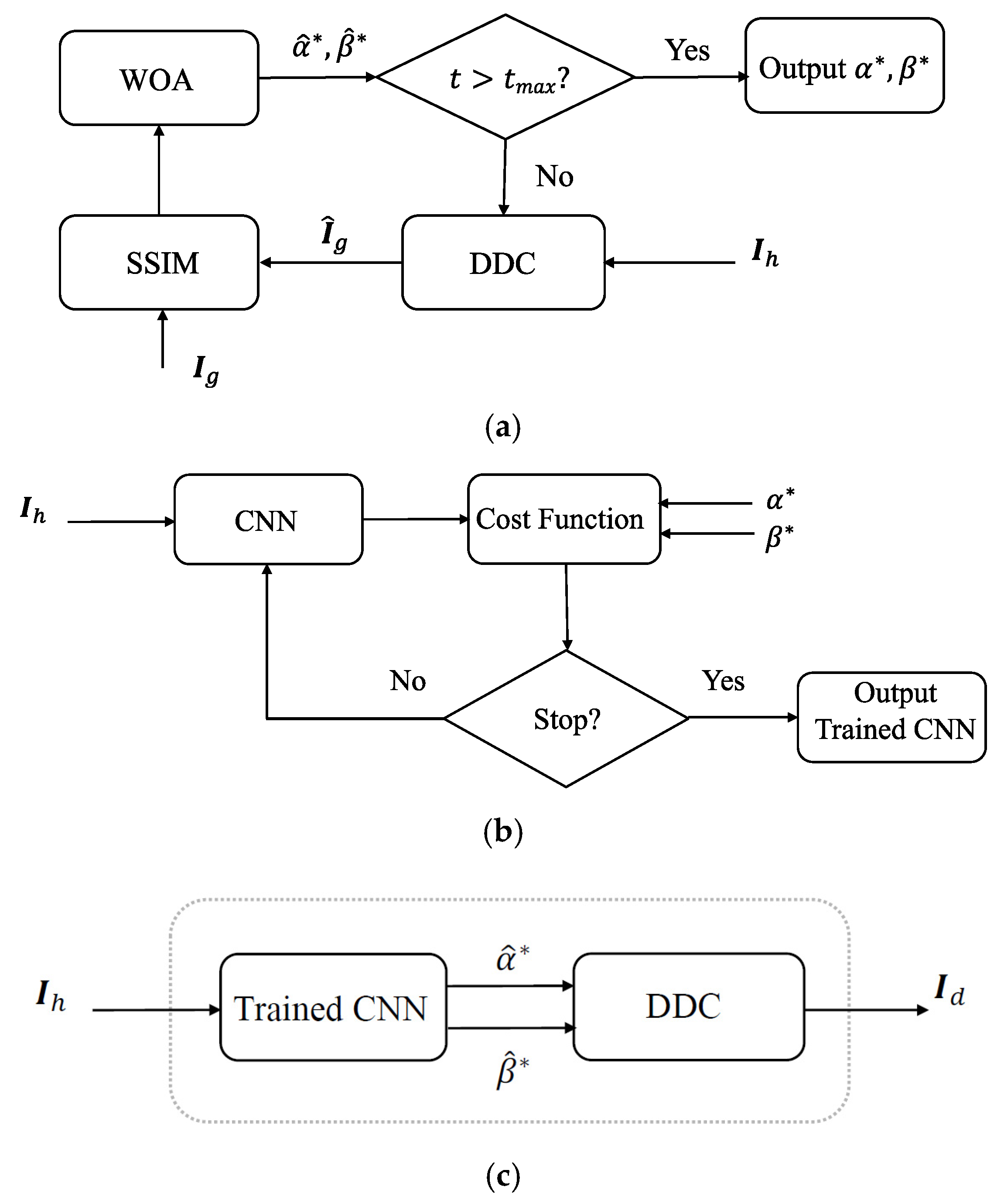
The proposed DDC_WOA_CNN method consists of three stages. In the first stage, for each input hazy image, the WOA is employed to find the optimal scaling factors: ${\alpha }^{\mathrm{*}}$ for $\mathit{A}$ and ${\beta }^{\mathrm{*}}$ for the initial transmittance $\tilde{t}(x)$ in the DDC. The method is referred to as the DDC_WOA, which establishes the mapping between hazy images and their corresponding optimal scaling factors. In the second stage, a CNN image regression model is used to learn the mapping obtained by the DDC_WOA. Finally, in the third stage, the DDC utilizes the optimal scaling factors estimated by the trained CNN, resulting in the proposed DDC_WOA_CNN method for practical applications. Figure 2 illustrates the block diagrams for the three stages, where ${\mathit{I}}_h$ represents a hazy image; ${\mathit{I}}_g$ is the ground-truth (GT) image; ${\mathit{I}}_d$ is the dehazed image, ${\widehat{\alpha }}^{\mathrm{*}}$ is an estimate of ${\alpha }^{\mathrm{*}}$ for atmospheric light $\mathit{A}$; and ${\widehat{\beta }}^{\mathrm{*}}$ is an estimate of ${\beta }^{\mathrm{*}}$ for initial transmittance $\tilde{t}(x)$. A detailed explanation of the proposed DDC, DDC_WOA, and DDC_WOA_CNN methods is provided in the next sections.

3.2. The DDC_WOA Scheme

This section describes how the WOA optimizes the scaling factors for $\mathit{A}$ and $\tilde{t}\left(x\right)$ in the DDC. The optimal scaling factors replace the adaptive ones mentioned in Section 2.2.3. Section 3.2.1 outlines the DDC_WOA scheme and discusses how hazy GT images impact its performance. Section 3.2.2 presents a solution to improve the performance of the DDC_WOA by incorporating haze level estimation.

3.2.1. Incorporating the WOA into the DDC

This section describes the use of the WOA to determine optimal scaling factors for $\mathit{A}$ and $\tilde{t}\left(x\right)$ in the DDC. The scheme is referred to as the DDC_WOA. The objective of the DDC_WOA is to map hazy images to their corresponding optimal scaling factors in the DDC. The resulting data are then used to train a CNN image regression model for learning the relationship between hazy images and their optimal scaling factors.

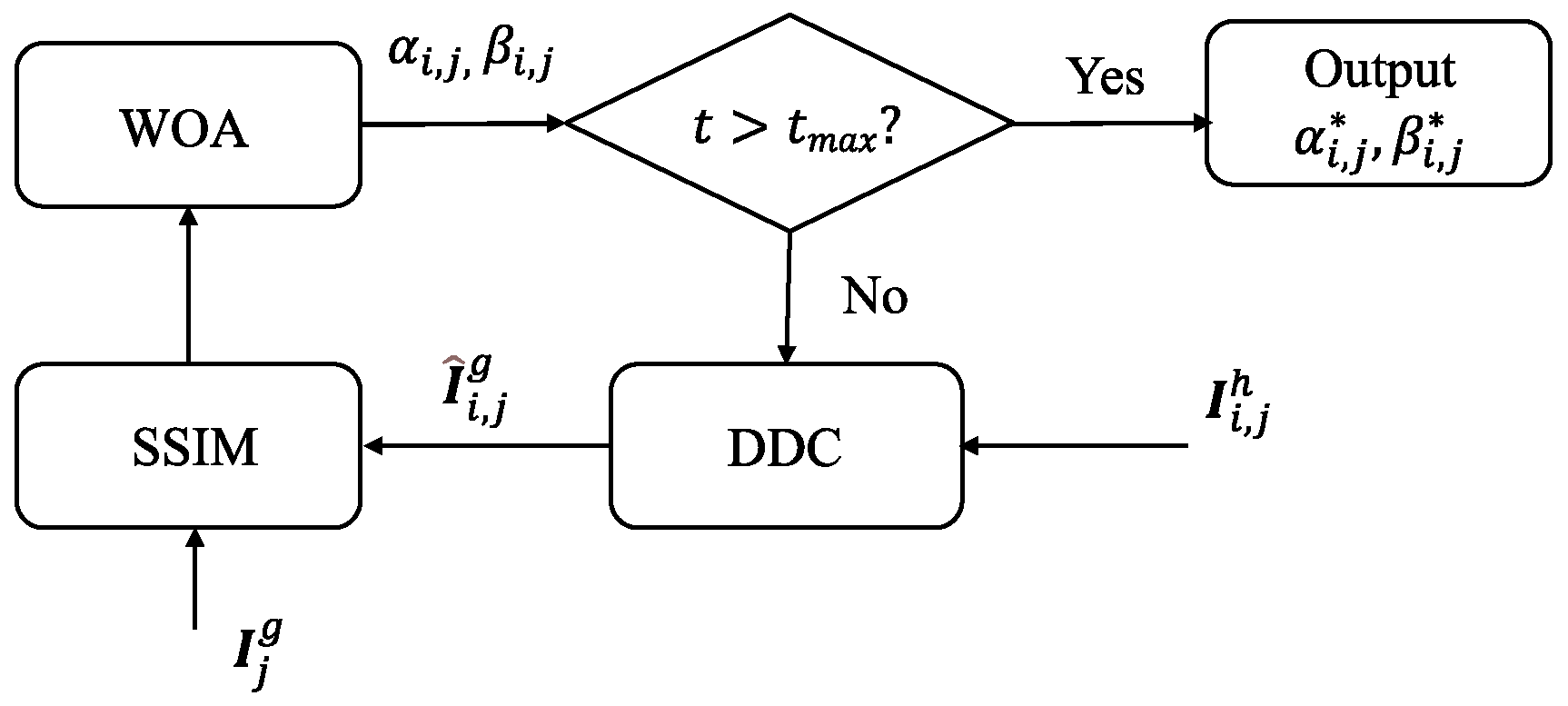
Let $\mathit{S}=\left\{\left({\mathit{I}}_{i,j}^h,{\mathit{I}}_j^g\right), \mathrm{f}\mathrm{o}\mathrm{r} 1\le i\le N_h,1\le j\le N_g\right\}$ denote a dataset of image pairs, where ${\mathit{I}}_{i,j}^h$ is a hazy image, and ${\mathit{I}}_j^g$ is the corresponding GT image; $N_h$ is the total number of hazy images; and $N_g$ is the total number of GT images. The RESIDE dataset in [37] is an example of this, where one GT image corresponds to 35 hazy images. The WOA is applied to each image pair $\left({\mathit{I}}_{i,j}^h,{\mathit{I}}_j^g\right)$ to find the optimal scaling factors ${\alpha }_{i,j}^{\mathrm{*}}$ and ${\beta }_{i,j}^{\mathrm{*}}$ in the DDC. In the searching process, the parameters $N_w=5$ (the number of whales) and $t_{max}=5$ (the maximum number of iterations) are used in the WOA, where the fitness function is the structure similarity (SSIM) [47]. Given ${\mathit{I}}_{i,j}^h$, the DDC generates a dehazed image ${\widehat{\mathit{I}}}_j^g$ using ${\alpha }_{i,j}$ and ${\beta }_{i,j}$ initially generated by the WOA. The SSIM is then computed between ${\widehat{\mathit{I}}}_j^g$ and ${\mathit{I}}_j^g$ to update ${\alpha }_{i,j}$ and ${\beta }_{i,j}$. This updating process occurs in each iteration of the WOA according to the SSIM values. The process continues until $t_{max}$ is reached. The resulting ${\alpha }_{i,j}$ and ${\beta }_{i,j}$ are then considered as the optimal scaling factors ${\alpha }_{i,j}^{\mathrm{*}}$ and ${\beta }_{i,j}^{\mathrm{*}}$ for ${\mathit{I}}_{i,j}^h$. Figure 3 illustrates the flow diagram of this process.

Note that the quality of GT images significantly impacts the dehazing performance of the DDC_WOA since the FRIQA SSIM is employed in the WOA.

Table 2. Images dehazed by the DDC_WOA with clear and hazy GT images.

GT Image	Input Hazy Image	Dehazed Image

demonstrates the impact of GT images on the DDC_WOA and indicates that a better dehazed image is obtained when a clear GT image is used (as shown in the first row), whereas the result is worse when a hazy GT image is used (as shown in the second row). This suggests that the quality of the dehazed image is directly related to the GT image utilized in the DDC_WOA. Therefore, selecting clear GT images is essential for accurately determining the optimal ${\alpha }_{i,j}^{*}$ and ${\beta }_{i,j}^{*}$ in the DDC_WOA. The next section presents a haze level estimation method for discriminating hazy GT images.

3.2.2. Hazy GT Image Discrimination

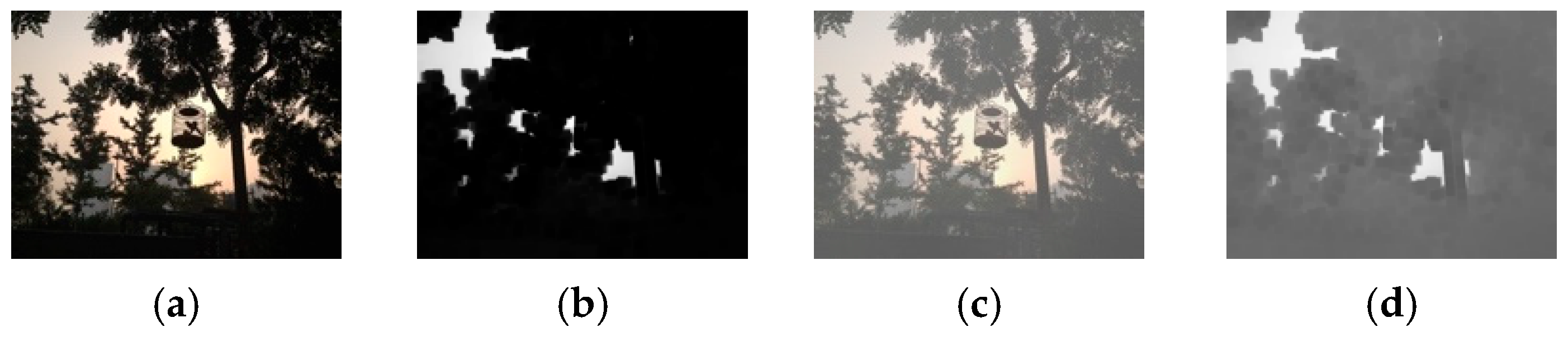
This section presents haze level estimation (HLE) through which a haze level indicator was developed to discriminate hazy GT images. The HLE is based on the dark channel prior in [9], which states that there are pixels with values zero or close to zero in a haze-free RGB image, excluding sky regions and white objects. A minimum filter can obtain the dark channel. Figure 4 shows a haze-free image, its generated hazy image, and the corresponding dark channels. A 15 × 15 minimum filter was used in this example. As one can see, the dark channel of the haze-free image in Figure 4b is darker than that of the hazy image in Figure 4d, except for the sky regions.

The result in Figure 4 suggests that the haze level in an image can be estimated through the dark channel, excluding sky regions and white objects. Therefore, a threshold $0<\mathsf{\tau }<1$ is introduced to exclude sky regions and white objects. Then, a truncated mean of the dark channel is calculated as an HL indicator. A smaller truncated mean implies that there is less haze in the image, and vice versa. Given an RGB image $\mathit{I}$, hazy GT image discrimination is implemented as follows:

Step 1.

Obtain the dark channel using the $15\times 15$ minimum filter as

$$I_{15}^{dark}(x)=\underset{y\in \mathsf{\Omega }\left(x\right)}{\min }\underset{c}{\min }\left[I_c\left(y\right)\right]$$

(22)

where $c\in \{R,G,B\}$ and $\mathsf{\Omega }\left(x\right)$ is a $15\times 15$ window centered at $x$.

Step 2.

Calculate a truncated mean of $I_{15}^{dark}(x)$ as

$${\tilde{\mu }}_{dc}\left(\tau \right)=\mathrm{m}\mathrm{e}\mathrm{a}\mathrm{n}[I_{15}^{dark}(x)\le \mathsf{\tau }]$$

(23)

where $0<\mathsf{\tau }<1$ is a user-defined threshold.

Step 3.

Check if the inequality ${\tilde{\mu }}_{dc}\left(\tau \right)<\eta$ holds, where $\eta$ is a user-defined threshold. If ${\tilde{\mu }}_{dc}\left(\tau \right)<\eta$, then $\mathit{I}$ is considered clear. Otherwise, go to Step 4.

Step 4.

Calculate the difference ${∆\tilde{\mu }}_{dc}={\tilde{\mu }}_{dc}\left({\tau }_1\right)-{\tilde{\mu }}_{dc}\left(\tau \right)$ and check if the inequality ${∆\tilde{\mu }}_{dc}<ϵ$ holds, where ${\tau }_1>\tau$ and $ϵ$ are user-defined thresholds. If ${∆\tilde{\mu }}_{dc}<ϵ$, then $\mathit{I}$ is considered clear; otherwise, it is hazy.

The algorithm is based on the following ideas: A clear GT image usually has less haze, and thus, ${\tilde{\mu }}_{dc}\left(0.4\right)$ is used as an HL indicator. If ${\tilde{\mu }}_{dc}\left(0.4\right)<\eta$, say 0.1, the GT image is clear. Otherwise, another check is performed. Through experiments, it is observed that ${\tilde{\mu }}_{dc}\left(\tau \right)$ changes little for a clear GT image as $\tau$ increases, but not for a hazy one. Therefore, the difference $∆{\tilde{\mu }}_{dc}={\tilde{\mu }}_{dc}\left(0.9\right)-{\tilde{\mu }}_{dc}\left(0.4\right)$ is used for the second check. A GT image is considered clear if $∆{\tilde{\mu }}_{dc}<ϵ$, say 0.1, and hazy otherwise. As a rule of thumb, the settings $\tau =0.4$, ${\tau }_1=0.9$, and $ϵ=0.1$ work well in most cases. However, it is noted that $\eta$ has a significant effect on the discrimination result. This will be further discussed in Section 4.1. Here, η equals 0.1 is used to demonstrate the feasibility of hazy GT image discrimination. Three GT images, denoted as ${\mathit{I}}_1$, ${\mathit{I}}_2$, and ${\mathit{I}}_3$, selected from the RESIDE dataset, are used as examples. They are shown in

Table 3. The ${\tilde{\mu }}_{dc}\left(\tau \right)$ for clear and hazy GT images as $\tau$ varies from 0.4 to 0.9.

	${\mathit{I}}_1$	${\mathit{I}}_2$	${\mathit{I}}_3$
Haze indicator
${\tilde{\mu }}_{dc}\left(0.9\right)$	0.0888	0.2742	0.3371
${\tilde{\mu }}_{dc}\left(0.8\right)$	0.0866	0.2742	0.3371
${\tilde{\mu }}_{dc}\left(0.7\right)$	0.0855	0.2742	0.3371
${\tilde{\mu }}_{dc}\left(0.6\right)$	0.0830	0.2721	0.3025
${\tilde{\mu }}_{dc}\left(0.5\right)$	0.0800	0.2613	0.2266
${\tilde{\mu }}_{dc}\left(0.4\right)$	0.0756	0.2461	0.1917
$∆{\tilde{\mu }}_{dc}$	0.0132	0.0281	0.1454

. The three images are discriminated as follows. Image ${\mathit{I}}_1$ is clear since ${\tilde{\mu }}_{dc}\left(0.4\right)=0.0756<0.1$. Image ${\mathit{I}}_2$ requires further verification since ${\tilde{\mu }}_{dc}\left(0.4\right)=0.2461>0.1$. The image is clear since $∆{\tilde{\mu }}_{dc}=0.0281<0.1$. Image ${\mathit{I}}_3$ is hazy for ${\tilde{\mu }}_{dc}\left(0.4\right)=0.1917>0.1$ and $∆{\tilde{\mu }}_{dc}=0.1454>0.1$. The result is consistent with the images shown in Table 3. In addition, ${\mathit{I}}_1$ and ${\mathit{I}}_2$ are considered clear images that have little change in ${\tilde{\mu }}_{dc}\left(\tau \right)$ as $\tau$ increases from 0.4 to 0.9. However, this is not the case for ${\mathit{I}}_3$, as described previously.

3.3. The CNN Image Regression Model

The DDC_WOA requires GT images to find the optimal scaling factors. However, GT images are not available in real-world applications. Therefore, the requirement for GT images needs to be relaxed. The DDC_WOA, fortunately, establishes mapping between hazy images and their optimal scaling factors. Thus, we used a CNN image regression model to learn the mapping. Once the mapping is learned, the need for GT images in the DDC_WOA is eliminated as the trained CNN can estimate optimal scaling factors for the DDC. The CNN image regression model in [48] was modified in this study by incorporating a dropout mechanism. It was then employed with a 50% drop rate. During the application stage, the trained CNN estimated the optimal scaling factors for a hazy input image, which were then used in the DDC to obtain dehazed images. The DDC with the estimated optimal scaling factors obtained from the trained CNN is referred to as DDC_WOA_CNN, as illustrated in Figure 2c. The proposed DDC_WOA_CNN approach can be used in practical applications.

4. Results and Discussion

This section justifies the proposed DDC_WOA_CNN method using the RESIDE [37] and KeDeMa [38] datasets. Section 4.1 outlines the preparation of experimental data from the RESIDE dataset. In Section 4.2, we compare the DCP, DDC, and DDC_WOA methods to demonstrate the superiority of the proposed DDC_WOA over the DCP and the DDC. Section 4.3 evaluates the proposed DDC_WOA_CNN method against four other dehazing methods: the GCAN [39] (an auto-encoder model), the RRO [12] (an optimized model-based method), the RFDN [40] (a weakly supervised model), and the Ka-Net (a transformer codec-based model) [41]. Finally, the results are discussed in Section 4.4.

4.1. Preparation of the RESIDE Dataset

This section describes the preparation of the RESIDE dataset for the following experiments. The RESIDE dataset comprises 8970 GT images (${\mathit{I}}_g$) and 313,950 hazy images (${\mathit{I}}_h$) generated from GT images. Each GT image with different model parameters in Equation (1) generated 35 hazy images. As mentioned in Section 3.2.2, not all GT images are clean. Thus, hazy GT image discrimination was applied to exclude hazy GT images and the corresponding generated hazy images. Empirically, the parameters $\tau$, ${\tau }_1$, and $ϵ$ in the discrimination were set to 0.4, 0.9, and 0.1, respectively. Since the parameter $\eta$ significantly affects the result, it must be appropriately determined.

Table 4. The results of GT image discrimination with various $\eta$ values for the RESIDE dataset.

$\eta$	0.1	0.075	0.05	0.025
$N_g$	4755	3902	3237	2984	8970
$N_h$	166,425	136,570	113,295	104,440	313,950

shows the results with different $\eta$ values, where $N_g$, $N_h$, and $p\%$ represent the number of GT images, the number of hazy images, and the percentage retained after discarding the image pairs with hazy GT images, respectively. The results show that many GT images are hazy in the RESIDE dataset. For example, only 53.01% of GT images are retained when $\eta =0.1$. To improve the performance of the DDC_WOA, the dataset with $\eta =0.025$ containing 2984 GT images and 104,440 hazy images was used in the following experiment. This dataset is denoted as $\mathit{S}(0.025)$.

4.2. Comparison of the DCP and Proposed DDC and DDC_WOA

This section compares the DCP and the proposed DDC and DDC_WOA. There are two purposes of this comparison. One is to show the superiority of the DDC over the DCP. The other is to demonstrate the benefit of using the WOA to find optimal scaling factors for the DDC. In the experiment, the DCP acts as a baseline to determine the improvement of the DDC and the DDC_WOA. Ten thousand images were randomly selected from $\mathit{S}(0.025)$. The DCP, DDC, and DDC_WOA were then used to find dehazed images. In the DDC_WOA, $N_w=10$ and $t_{max}=20$ were used in the WOA.

In the experiments, four objective image quality assessments (IQAs) were used to evaluate dehazed images. They are the SSIM [45], the peak signal-to-noise ratio (PSNR), the ILNIQE [47], and the DHQI [49]. The SSIM and PSNR are full-reference IQAs (FRIQAs), and the ILNIQE and the DHQI are no-reference IQAs (NRIQAs). The reason for using four IQAs is that it is well-known that each IQA has its own preferences. Additionally, FRIQAs are more reliable than NRIQAs since they use GT images as references. It should also be noted that a better NRIQA may not necessarily be consistent with visual quality, as NRIQAs may fail in some cases. Thus, a subjective (visual) quality evaluation is required in fields of image processing, such as image dehazing. For a comprehensive survey on IQAs, see [50].

The IQA results are shown in

Table 5. Objective comparison of the DCP and proposed DDC and DDC_WOA (RESIDE).

	DCP	DDC	DDC_WOA
SSIM ↑	0.879 (3)	0.917 (2)	0.941 (1)
PSNR ↑	18.295 (3)	23.807 (2)	29.016 (1)
ILNIQE ↓	20.666 (2)	21.549 (3)	20.567 (1)
DHQI ↓	50.856 (1)	55.386 (3)	55.256 (2)
$\overline{R}$ ↓	2.25	2.50	1.25

, where the arrow indicates the better direction, and the number in the parentheses is the rank for that IQA. The average rank is denoted as $\overline{R}$, which is used as an overall performance index. In the case of the SSIM, the DDC_WOA outperforms the DCP and the DDC by 0.062 and 0.024, respectively. The DDC has a better SSIM than the DCP by 0.038. Regarding the PSNR, the DDC_WOA significantly outperforms the DCP and the DDC by 10.721 dB and 5.209 dB, respectively. The DDC is better than the DCP by 5.512 dB. In other words, the estimation of $\mathit{A}$ and $t(x)$ in the DDC is more appropriate than that in the DCP. Additionally, the DDC_WOA achieves a better PSNR than the DDC by 5.209 dB. This indicates that the DDC has been significantly improved by introducing the WOA to search for optimal scaling factors. Regarding the ILNIQE, the DDC_WOA outperforms the DCP and the DDC by −0.099 and −0.982, respectively. The DCP has a better ILNIQE than the DDC by −0.883. In the case of the DHQI, the DDC_WOA is inferior to the DCP by 4.4 and is better than the DDC by −0.13, respectively. As for the overall performance index $\overline{R}$, the DDC_WOA has the best value (1.25), followed by the DCP (2.25) and the DDC (2.50). Though the $\overline{R}$ of the DDC is worse than that of the DCP, the DDC still has better visual quality, as evidenced in the FRIQAs, i.e., the SSIM and the PSNR. The DDC_WOA has the best performance for the SSIM and the PSNR, and thus, the best visual quality is expected. This implies that FRIQAs are more reliable than the NRIQAs, which is confirmed by the following subjective comparison.

Four dehazed images produced by the DCP, DDC, and DDC_WOA were selected for subjective comparison. They are shown in

Table 6. Subjective comparison of the DCP and proposed DDC and DDC_WOA (RESIDE).

(a)
	${\mathit{I}}_{\mathit{g}}$	${\mathit{I}}_{\mathit{h}}$	DCP	DDC	DDC_WOA
${\mathit{I}}_1$
${\mathit{I}}_2$
${\mathit{I}}_3$
${\mathit{I}}_4$
(b). Subjective comparison of Table 6a with zoomed patches.
	${\mathit{I}}_g$	${\mathit{I}}_h$	DCP	DDC	DDC_WOA
${\mathit{I}}_1$
${\mathit{I}}_2$
${\mathit{I}}_3$
${\mathit{I}}_4$

a, where the corresponding GT image and hazy image are included for reference. Table 6b shows the zoomed image patches for the images shown in Table 6a for easier observation. The DCP exhibits artifacts in the sky regions of ${\mathit{I}}_1$ and ${\mathit{I}}_4$; halos around the eaves in ${\mathit{I}}_2$; and color distortion in the sky regions of ${\mathit{I}}_2$ and ${\mathit{I}}_3$. The DDC has much better visual quality than the DCP. The DDC_WOA outperforms the DDC in the visual quality of dehazed images. As expected, the result confirms that the DDC_WOA enhances the performance of the DDC by replacing ${\alpha }_a$ and ${\beta }_a$ with the optimal scaling factors ${\alpha }^{\mathrm{*}}$ and ${\beta }^{\mathrm{*}}$.

This section has shown that the DDC_WOA has the best performance in the comparison. However, GT images are required in the DDC_WOA, so this method cannot be used in real-world applications. To address the problem, a CNN image regression model was used to learn the mapping between input hazy images and their optimal scaling factors. The trained CNN was then used to estimate the optimal scaling factors for a hazy image input to the DDC. The resulting DDC_WOA_CNN method, shown in Figure 2c, was used in subsequent experiments. The proposed DDC_WOA_CNN method was trained using 10,000 randomly selected images from $\mathit{S}(0.025)$, which is a different subset from the testing subset in subsequent experiments.

4.3. Comparison of the DDC_WOA_CNN Approach and Four Dehazing Methods

This section compares the dehazing performance of the proposed DDC_WOA_CNN method with that of the GCAN (an autoencoder model) [39], the RRO (an optimized model-based method) [12], the RFDN (a weakly supervised model) [40], and the Ka-Net (a transformer codec-based network) [41]. A subset of $\mathit{S}(0.025)$ and the KeDeMa dataset [38] were used in the experiment. Section 4.3.1 presents the results for the RESIDE dataset, while Section 4.3.2 presents the results for the KeDeMa dataset.

4.3.1. Results for the RESIDE Dataset

The performance of the proposed DDC_WOA_CNN method was investigated using the RESIDE dataset. In the experiment, 10,000 hazy images were randomly selected from $\mathit{S}(0.025)$ as a testing dataset. The DDC_WOA_CNN, GCAN, RRO, RFDN, and Ka-Net methods were then applied to obtain dehazed images. Then, the four objective IQAs mentioned in Section 4.2 were used to evaluate the performance of each method.

Table 7. Objective comparison for the proposed DDC_WOA_CNN, GCAN, RRO, RFDN, and Ka-Net methods (RESIDE).

	DDC_WOA_CNN	GCAN	RRO	RFDN	Ka-Net
SSIM ↑	0.936 (1)	0.912 (3)	0.889 (4)	0.933 (2)	0.601 (5)
PSNR ↑	26.984 (1)	24.975 (2)	20.942 (4)	23.496 (3)	18.009 (5)
ILNIQE ↓	20.709 (2)	21.351 (4)	20.856 (3)	19.831 (1)	21.500 (5)
DHQI ↓	55.391 (5)	54.997 (4)	52.029 (2)	52.638 (3)	43.265 (1)
$\overline{R}$ ↓	2.25	3.25	3.25	2.25	4

shows the evaluation results. It indicates that the proposed DDC_WOA_CNN method achieves a better SSIM than the GCAN, RRO, RFDN, and Ka-Net by 0.024, 0.047, 0.003, and 0.335, respectively. In the case of the PSNR, the DDC_WOA_CNN approach has a better result than the GCAN, RRO, RFDN, and Ka-Net by 2.009 dB, 6.042 dB, 3.488 dB, and 8.975 dB, respectively. Regarding the ILNIQE, the best result is achieved by the RFDN (19.831), followed by the DDC_WOA_CNN method (20.709), RRO (20.856), GCAN (21.351), and Ka-Net (21.500). The Ka-Net has the best result (43.265) for the DHQI, followed by the RRO (52.029), RFDN (52.638), GCAN (54.997), and DDC_WOA_CNN method (55.391). Although the DDC_WOA_CNN approach and the RFDN have the same $\overline{R}$, it has better visual quality. As described previously, the FRIQAs (SSIM and PSNR) are more reliable than the NRIQAs (ILNIQE and DHQI) because FRIQAs use GT images as references. Thus, the dehazed images of the DDC_WOA_CNN method are expected to have better visual quality. This is verified below.

Next, eight dehazed images were selected for comparison of the visual quality of dehazed images obtained with the DDC_WOA_CNN method and the other four comparison methods. The images, denoted as ${\mathit{I}}_1$ to ${\mathit{I}}_8$, were purposely selected with various haze levels. They are presented in

Table 8. Subjective comparison of the proposed DDC_WOA_CNN, GCAN, RRO, RFDN, and Ka-Net methods (RESIDE).

(a)
	${\mathit{I}}_{\mathit{g}}$	${\mathit{I}}_{\mathit{h}}$ ${\tilde{\mathit{\mu }}}_{\mathit{d}\mathit{c}}(0.8)$	DDC_WOA_CNN	GCAN	RRO	RFDN	Ka-Net
${\mathit{I}}_1$
PSNR	1708_0.85_0.08	0.249	29.165	27.382	16.812	22.254	13.921
${\mathit{I}}_2$
PSNR	7556_0.85_0.06	0.324	22.599	18.416	17.118	19.277	16.682
${\mathit{I}}_3$
PSNR	8694_0.8_0.04	0.282	27.819	23.955	18.830	19.784	12.592
${\mathit{I}}_4$
PSNR	0639_1_0.08	0.406	25.610	25.904	19.488	18.362	15.432
${\mathit{I}}_5$
PSNR	0822_1_0.06	0.336	27.201	17.135	20.322	19.828	18.595
${\mathit{I}}_6$
PSNR	8118_0.85_0.2	0.479	26.438	25.420	17.866	21.404	18.379
${\mathit{I}}_7$
PSNR	8813_0.8_0.08	0.428	25.221	20.644	20.829	19.640	15.661
${\mathit{I}}_8$
PSNR	1781_1_0.2	0.546	24.241	23.870	18.413	21.698	16.995
(b). Subjective comparison of Table 8a with zoomed patches.
	${\mathit{I}}_g$	${\mathit{I}}_h$ ${\tilde{\mu }}_{dc}(0.8)$	DDC_WOA_CNN	GCAN	RRO	RFDN	Ka-Net
${\mathit{I}}_1$
PSNR	1708_0.85_0.08	0.249	29.165	27.382	16.812	22.254	13.921
${\mathit{I}}_2$
PSNR	7556_0.85_0.06	0.324	22.599	18.416	17.118	19.277	16.682
${\mathit{I}}_3$
PSNR	8694_0.8_0.04	0.282	27.819	23.955	18.830	19.784	12.592
${\mathit{I}}_4$
PSNR	0639_1_0.08	0.406	25.610	25.904	19.488	18.362	15.432
${\mathit{I}}_5$
PSNR	0822_1_0.06	0.336	27.201	17.135	20.322	19.828	18.595
${\mathit{I}}_6$
PSNR	8118_0.85_0.2	0.479	26.438	25.420	17.866	21.404	18.379
${\mathit{I}}_7$
PSNR	8813_0.8_0.08	0.428	25.221	20.644	20.829	19.640	15.661
${\mathit{I}}_8$
PSNR	1781_1_0.2	0.546	24.241	23.870	18.413	21.698	16.995

a, where the image filename, the haze level ${\tilde{\mu }}_{dc}(0.8)$, and the PSNR values for each dehazed image are given for reference. Moreover, ${\mathit{I}}_g$ and ${\mathit{I}}_h$ in Table 8a represent the GT image and hazy image, respectively. The related zoomed image patches are shown in Table 8b for clearer observation. According to Table 8a, the GCAN exhibits artifacts and color distortion in the sky regions of ${\mathit{I}}_5$ and ${\mathit{I}}_7$. The RRO presents artifacts, color distortion, or both in the sky regions of ${\mathit{I}}_1$, ${\mathit{I}}_3$, ${\mathit{I}}_5$, ${\mathit{I}}_7$, and ${\mathit{I}}_8$. The RFDN introduces artifacts and color distortion in the sky regions of ${\mathit{I}}_3$, ${\mathit{I}}_5$, and ${\mathit{I}}_7$. The proposed DDC_WOA_CNN method avoids the above problems. That is, our method generally has the best visual quality in the given examples, as expected. Additionally, the subjective results are consistent with the PSNR given in Table 8a. This suggests that FRIQAs are more reliable than NRIQAs, as mentioned before.

Finally, the efficiency of the above-mentioned methods was compared. The results are presented in

Table 9. Efficiency comparison of the proposed DDC_WOA_CNN, GCAN, RRO, RFDN, and Ka-Net methods (RESIDE).

	DDC_WOA_CNN	GCAN	RRO	RFDN	Ka-Net
$\overline{t}$	0.343	0.147	0.763	1.571	0.085
$∆\overline{t}$	0	+0.196	−0.420	−1.228	+0.258

, where the time represents the average runtime for processing an image (in seconds/image), denoted as $\overline{t}$. In Table 9, the descending rank of the runtime $\overline{t}$ is Ka-Net, GCAN, the proposed DDC_WOA_CNN, RRO, and RFDN. The difference in $\overline{t}$ between the proposed DDC_WOA_CNN approach and other comparison methods is $∆\overline{t}={\overline{t}}_r-{\overline{t}}_c$, where ${\overline{t}}_r$ is the runtime of the DDC_WOA_CNN method, and ${\overline{t}}_c$ is that for a comparison method. As shown in Table 9, the $\overline{t}$ for our approach is 0.343 s/image. It meets the requirements of most real-world applications despite not having the best performance. The GCAN is more efficient than our method; however, it yields poor visual results, as indicated in Table 8. In summary, the proposed approach exhibits mild efficiency but offers better visual quality in dehazed images compared to the other methods in the given examples.

4.3.2. Results for the KeDeMa Dataset

The proposed DDC_WOA_CNN method was further investigated using the KeDeMa dataset. It was compared with the four comparison methods as before. The KeDeMa dataset consists of 25 natural images with different scenes and haze levels, where no GT images are provided. Therefore, it is impossible to calculate the FRIQAs (SSIM and PSNR), only the NRIQAs (ILNIQE and DHQI). The results of the DDC_WOA_CNN approach and the four comparison methods are shown in

Table 10. Objective comparison of the proposed DDC_WOA_CNN, GCAN, RRO, RFDN, and Ka-Net methods (KeDeMa).

	DDC_WOA_CNN	GCAN	RRO	RFDN	Ka-Net
ILNIQE ↓	26.131 (4)	26.298 (5)	23.855 (2)	23.434 (1)	24.857 (3)
DHQI ↓	62.347 (4)	50.234 (2)	62.934 (5)	48.253 (1)	50.522 (3)
$\overline{R}$ ↓	4	3.5	3.5	1	3

.

In the ILNIQE, the rank order of $\overline{R}$, from top to bottom, is RFDN, Ka-Net, RRO, and DDC_WOA_CNN, where the GCAN has the same rank as the RRO. As for the DHQI, the ranking order is RFDN, GCAN, Ka-Net, DDC_WOA_CNN, and RRO. Although our method has the worst $\overline{R}$, this does not mean poor visual quality of dehazed images, as confirmed in the visual evaluation below.

NRIQAs (ILNIQE and DHQI) cannot appropriately reflect the visual quality of dehazed images as described before. Thus, ten dehazed images were selected from five different categories (architecture, human, landscape, night image, and plant) in the KeDeMa for subjective comparison. They are shown in

Table 11. Subjective comparison of the proposed DDC_WOA_CNN, GCAN, RRO, RFDN, and Ka-Net methods (KeDeMa).

(a)
	${\mathit{I}}_{\mathit{h}}$ ${\tilde{\mathit{\mu }}}_{\mathit{d}\mathit{c}}(\mathbf{0.8})$	DDC_WOA_ CNN	GCAN	RRO	RFDN	Ka-Net
${\mathit{I}}_1$
DHQI/ILNIQE	architecture1 0.410	58.607/29.591	53.134/25.372	54.915/26.314	58.517/24.817	49.084/28.340
${\mathit{I}}_2$
DHQI/ILNIQE	architecture2 0.633	62.307/29.396	62.554/26.473	59.026/26.802	60.605/24.252	44.312/30.238
${\mathit{I}}_3$
DHQI/ILNIQE	human1 0.365	65.538/19.403	64.922/21.870	65.015/17.463	62.809/18.524	57.947/22.122
${\mathit{I}}_4$
DHQI/ILNIQE	human2 0.506	60.299/27.849	53.728/27.784	56.274/25.780	50.818/24.525	47.375/24.744
${\mathit{I}}_5$
DHQI/ILNIQE	landscape1 0.461	62.357/30.789	64.124/28.496	59.318/28.336	59.740/24.111	56.268/27.660
${\mathit{I}}_6$
DHQI/ILNIQE	landscape2 0.345	63.650/21.956	58.934/29.138	58.864/18.951	53.443/21.734	54.450/21.394
${\mathit{I}}_7$
DHQI/ILNIQE	night1 0.214	52.694/32.682	52.346/30.242	52.966/30.039	50.723/29.770	45.796/45.796
${\mathit{I}}_8$
DHQI/ILNIQE	night2 0.157	57.965/27.910	59.257/24.839	60.181/22.774	58.865/22.947	50.868/23.573
${\mathit{I}}_9$
DHQI/ILNIQE	plant3 0.319	63.201/33.499	60.128/33.996	59.121/30.868	60.218/28.597	46.245/28.107
${\mathit{I}}_{10}$
DHQI/ILNIQE	plant4 0.695	55.981/27.303	46.314/27.620	43.809/25.297	47.830/24.356	42.847/29.195
(b). Subjective comparison of Table 11a with zoomed patches.
	${\mathit{I}}_h$ ${\tilde{\mu }}_{dc}(0.8)$	DDC_WOA_ CNN	GCAN	RRO	RFDN	Ka-Net
${\mathit{I}}_1$
DHQI/ILNIQE	architecture1 0.410	58.607/29.591	53.134/25.372	54.915/26.314	58.517/24.817	49.084/28.340
${\mathit{I}}_2$
DHQI/ILNIQE	architecture2 0.633	62.307/29.396	62.554/26.473	59.026/26.802	60.605/24.252	44.312/30.238
${\mathit{I}}_3$
DHQI/ILNIQE	human1 0.365	65.538/19.403	64.922/21.870	65.015/17.463	62.809/18.524	57.947/22.122
${\mathit{I}}_4$
DHQI/ILNIQE	human2 0.506	60.299/27.849	53.728/27.784	56.274/25.780	50.818/24.525	47.375/24.744
${\mathit{I}}_5$
DHQI/ILNIQE	landscape1 0.461	62.357/30.789	64.124/28.496	59.318/28.336	59.740/24.111	56.268/27.660
${\mathit{I}}_6$
DHQI/ILNIQE	landscape2 0.345	63.650/21.956	58.934/29.138	58.864/18.951	53.443/21.734	54.450/21.394
${\mathit{I}}_7$
DHQI/ILNIQE	night1 0.214	52.694/32.682	52.346/30.242	52.966/30.039	50.723/29.770	45.796/45.796
${\mathit{I}}_8$
DHQI/ILNIQE	night2 0.157	57.965/27.910	59.257/24.839	60.181/22.774	58.865/22.947	50.868/23.573
${\mathit{I}}_9$
DHQI/ILNIQE	plant3 0.319	63.201/33.499	60.128/33.996	59.121/30.868	60.218/28.597	46.245/28.107
${\mathit{I}}_{10}$
DHQI/ILNIQE	plant4 0.695	55.981/27.303	46.314/27.620	43.809/25.297	47.830/24.356	42.847/29.195

a, where the corresponding values of the ILNIQE, DHQI, and haze level ${\tilde{\mu }}_{dc}(0.8)$ are given for reference. The zoomed image patches of the dehazed images are presented in Table 11b for easier observation. Table 11a shows that the GCAN exhibits color distortion in ${\mathit{I}}_2$, ${\mathit{I}}_4$, ${\mathit{I}}_6$, and ${\mathit{I}}_{10}$, whereas artifacts are found in the sky region of ${\mathit{I}}_1$. The RRO performs reasonably well. However, it exhibits artifacts and color distortion in the sky regions of ${\mathit{I}}_6$ and ${\mathit{I}}_{10}$. In the case of the RFDN, color oversaturation is observed in ${\mathit{I}}_3$, while an artifact is found in the center of the moon in ${\mathit{I}}_7$. Regarding the Ka-Net, halos appear around the policemen in ${\mathit{I}}_4$. Our DDC_WOA_CNN approach generally shows excellent visual quality in the given examples. In summary, the visual results indicate that the NRIQAs (ILNIQE and DHQI) are inconsistent with the subjective comparison, i.e., a lower value of the ILNIQE or DHQI does not mean better visual quality. This again suggests that FRIQAs are more reliable than NRIQAs.

4.4. Discussion

At least three points should be mentioned for the results in Section 4.3. First, the performance of the proposed DDC is much better than that of the DCP (5.512 dB in PSNR, Table 5). This proves the DDC is feasible and promising. Second, the DDC_WOA significantly improves the DDC (5.209 dB in PSNR, Table 5). That is, the optimized scaling factors in the DDC_WOA outperform the empirical ones in the DDC, as expected. The usage of the WOA in the DDC_WOA provides an alternative way to apply an optimization algorithm in model-based dehazing methods. Third, the proposed DDC_WOA_CNN method is generally visually superior to the comparison end-to-end methods, i.e., the GCAN, RFDN, and Ka-Net. This implies that model-based dehazing methods can be more effective than data-driven models when model parameters are appropriately estimated.

The proposed approach was verified using a synthesized image dataset (RESIDE) and a natural image dataset (KeDeMa). Our method generally yielded superior visual results compared to the comparison methods. However, the NRIQAs (DHQI and ILNIQE) are inconsistent with the visual evaluation, e.g., in Table 8 and Table 11. The DHQI is designed to evaluate the quality of dehazed images. It considers three features in a dehazed image, i.e., haze removal, structure preservation, and over-enhancement. However, it is inconsistent with the visual evaluation in the given examples. The reason might be that the DHQI has insufficient data in training to learn the visual properties of the dehazed image. The ILNIQE utilizes five natural scene statistics features from pristine image patches: normalized luminance, mean-subtracted and contrast-normalized coefficient products, gradient, log-Gabor filter response, and colors. The features are then used to construct a multivariate Gaussian model, which serves as a pristine reference against which test image quality is measured. In the given examples, the ILNIQE is inconsistent with the visual evaluation. This might be explained by the dehazed images falling outside of the learned distribution of pristine image patches in the ILNIQE.

FRIQAs have better performance than NRIQAs because they use GT images as references. However, the GT images are not available in real-world scenarios. NRIQAs are thus needed since they do not require GT images. More reliable NRIQAs need to be sought since current NRIQAs are incapable of handling some cases, as shown in Table 7 and Table 11. An NRIQA that is consistent with the visual evaluation should consequently be investigated in future research.

5. Conclusions and Further Research

This paper has presented a dehazing method called DDC_WOA_CNN, which was developed in three stages: (i) the development of a dehazing scheme based on dual dark channels, which is called the DDC; (ii) the use of the WOA to search for optimal scaling factors for atmospheric light and initial transmittance in the DDC, which is called the DDC_WOA; (iii) the implementation of a CNN image regression model to learn the relationship between hazy images and their optimized scaling factors obtained from the DDC_WOA. The trained CNN was then used to estimate the optimal scaling factors for the DDC to obtain dehazed images. This approach makes the proposed DDC_WOA_CNN method applicable in real-world scenarios. The DDC_WOA_CNN method was verified using the RESIDE and KeDeMa image datasets. Furthermore, it was compared with four other dehazing methods: the GCAN, RRO, RFDN, and Ka-Net. For the RESIDE dataset, the results indicate that DDC_WOA_CNN outperforms the GCAN by 2.009 dB, the RRO by 6.042 dB, the RFDN by 3.488 dB, and the Ka-Net by 8.975, in terms of the PSNR. Moreover, the DDC_WOA_CNN method generally has the best visual quality among the comparison methods. As for the natural image dataset KeDeMa, the proposed DDC_WOA_CNN approach also generally demonstrated superior visual quality compared to the four comparison methods.

Although the DDC_WOA_CNN method achieved excellent performance, there are at least four points that should be further improved. First, the scaling factors ${\alpha }_a$ and ${\beta }_a$ in the proposed DDC described in Section 2.2.3 were empirically determined. Their theoretical justification will be the subject of future research. Second, the $w(x)$ used to estimate the initial transmittance $\tilde{t}(x)$ was determined in our experiments. In further research, a derivation of this linear relationship from the physical scattering model will be investigated to provide rigorous support. Third, an NRIQA will be investigated for image dehazing, ensuring that the objective evaluation is consistent with the subjective evaluation. Fourth, approximately 2 dB in the PSNR is lost during the learning process of the CNN image regression model. Thus, further research will also focus on minimizing this loss to improve the proposed DDC_WOA_CNN method.

References

1. Gui, J.; Cong, X.; Cao, Y.; Ren, W.; Zhang, J.; Zhang, J.; Cao, J.; Tao, D. A Comprehensive Survey and Taxonomy on Single Image Dehazing Based on Deep Learning. ACM Comput. Surv. 2023, 55, 1–37. [Google Scholar] [CrossRef]
2. Ayoub, A.; El-Shafai, W.; El-Samie, F.E.A.; Hamad, E.K.I.; El-Rabaie, E.-S.M. Review of Dehazing Techniques: Challenges and Future Trends. Multimed. Tools Appl. 2025, 84, 1103–1131. [Google Scholar] [CrossRef]
3. Pandey, P.; Gupta, R.; Goel, N. Comprehensive Review of Single Image Defogging Techniques: Enhancement, Prior, and Learning Based Approaches. Artif. Intell. Rev. 2025, 58, 116. [Google Scholar] [CrossRef]
4. Narasimhan, S.G.; Nayar, S.K. Vision and the Atmosphere. Int. J. Comput. Vis. 2002, 48, 233–254. [Google Scholar] [CrossRef]
5. Fattal, R. Single Image Dehazing. ACM Trans. Graph. 2008, 27, 721–729. [Google Scholar] [CrossRef]
6. Fattal, R. Dehazing Using Color-Lines. ACM Trans. Graph. 2015, 34, 1–14. [Google Scholar] [CrossRef]
7. Zhu, Q.; Mai, J.; Shao, L. A Fast Single Image Haze Removal Algorithm Using Color Attenuation Prior. IEEE Trans. Image Process. 2015, 24, 3522–3533. [Google Scholar] [CrossRef]
8. Cai, B.; Xu, X.; Jia, K.; Qing, C.; Tao, D. DehazeNet: An End-to-End System for Single Image Haze Removal. IEEE Trans. Image Process. 2016, 25, 5187–5198. [Google Scholar] [CrossRef]
9. He, K.; Sun, J.; Tang, X. Single Image Haze Removal Using Dark Channel Prior. IEEE Trans. Pattern Anal. Mach. Intell. 2011, 33, 2341–2353. [Google Scholar]
10. Wang, J.; Lu, K.; Xue, J.; He, N.; Shao, L. Single Image Dehazing Based on the Physical Model and MSRCR Algorithm. IEEE Trans. Circuits Syst. Video Technol. 2018, 28, 2190–2199. [Google Scholar] [CrossRef]
11. Hsieh, C.-H.; Chen, J.-Y.; Zhao, Q. A Modified DCP Based Dehazing Algorithm. In Proceedings of the 2018 IEEE International Conference on Systems, Man, and Cybernetics (SMC), Miyazaki, Japan, 7–10 October 2018; pp. 1779–1784. [Google Scholar] [CrossRef]
12. Shin, J.; Kim, M.; Paik, J.; Lee, S. Radiance–Reflectance Combined Optimization and Structure-Guided 0-Norm for Single Image Dehazing. IEEE Trans. Multimed. 2020, 22, 30–44. [Google Scholar] [CrossRef]
13. Raikwar, S.C.; Tapaswi, S. Lower Bound on Transmission Using Non-Linear Bounding Function in Single Image Dehazing. IEEE Trans. Image Process. 2020, 29, 4832–4847. [Google Scholar] [CrossRef] [PubMed]
14. Salazar-Colores, S.; Moya-Sánchez, E.U.; Ramos-Arreguín, J.-M.; Cabal-Yépez, E.; Flores, G.; Cortés, U. Fast Single Image Defogging with Robust Sky Detection. IEEE Access 2020, 8, 149176–149189. [Google Scholar] [CrossRef]
15. Zhou, H.; Yuan, C.; Pan, H.; Yang, Y.; Wang, Z.; Chen, X. Image Dehazing Algorithm Based on Particle Swarm Optimization for Sky Region Segmentation. In Proceedings of the 2022 21st International Symposium on Distributed Computing and Applications for Business Engineering and Science (DCABES), Chizhou, China, 14–18 October 2022; pp. 132–135. [Google Scholar] [CrossRef]
16. Li, B.; Peng, X.; Wang, Z.; Xu, J.; Feng, D. AOD-Net: All-in-One Dehazing Network. In Proceedings of the 2017 IEEE International Conference on Computer Vision (ICCV), Venice, Italy, 22–29 October 2017; pp. 4780–4788. [Google Scholar] [CrossRef]
17. Chen, S.; Cheng, J.; Huang, Z. GADO-Net: An Improved AOD-Net Single Image Dehazing Algorithm. In Proceedings of the 2021 3rd International Academic Exchange Conference on Science and Technology Innovation (IAECST), Guangzhou, China, 10–12 December 2021; pp. 640–646. [Google Scholar] [CrossRef]
18. Luan, Z.; Shang, Y.; Zhou, X.; Shao, Z.; Guo, G.; Liu, X. Fast Single Image Dehazing Based on a Regression Model. Neurocomputing 2017, 245, 10–22. [Google Scholar] [CrossRef]
19. Golts, A.; Freedman, D.; Elad, M. Unsupervised Single Image Dehazing Using Dark Channel Prior Loss. IEEE Trans. Image Process. 2020, 29, 2692–2701. [Google Scholar] [CrossRef]
20. Chen, W.-T.; Fang, H.-Y.; Ding, J.-J.; Kuo, S.-Y. PMHLD: Patch Map-Based Hybrid Learning DehazeNet for Single Image Haze Removal. IEEE Trans. Image Process. 2020, 29, 6773–6788. [Google Scholar] [CrossRef]
21. Li, Z.; Zheng, C.; Shu, H.; Wu, S. Single Image Dehazing via Model-Based Deep-Learning. In Proceedings of the 2022 IEEE International Conference on Image Processing (ICIP), Bordeaux, France, 16–19 October 2022; pp. 141–145. [Google Scholar]
22. Asha, C.S.; Siddiq, A.B.; Akthar, R.; Rajan, M.R.; Suresh, S. ODD-Net: A Hybrid Deep Learning Architecture for Image Dehazing. Sci. Rep. 2024, 14, 30619. [Google Scholar] [CrossRef]
23. Yeh, C.-H.; Kang, L.-W.; Lin, C.-Y.; Lin, C.-Y. Efficient image/Video Dehazing Through Haze Density Analysis Based on Pixel-Based Dark Channel Prior. In Proceedings of the 2012 International Conference on Information Security and Intelligent Control, Yunlin, Taiwan, 14–16 August 2012; pp. 238–241. [Google Scholar] [CrossRef]
24. Zeng, Y.; Liu, X. A Multi-Scale Fusion-Based Dark Channel Prior Dehazing Algorithm. In Proceedings of the Sixth International Conference on Graphic and Image Processing (ICGIP 2014), SPIE 9443, Beijing, China, 24–26 October 2014; pp. 284–290. [Google Scholar]
25. Hsieh, C.-H.; Zhao, Q.; Cheng, W.-C. Single Image Haze Removal Using Weak Dark Channel Prior. In Proceedings of the 2018 9th International Conference on Awareness Science and Technology (iCAST), Fukuoka, Japan, 19–21 September 2018; pp. 214–219. [Google Scholar] [CrossRef]
26. Nair, S.; Menon, S.; Karlekar, M.; Prasad, M.T.; Rashmi, M. Single Image Dehazing Using Multi-Scale DCP-BCP Fusion. In Proceedings of the 2022 Second International Conference on Advanced Technologies in Intelligent Control, Environment, Computing & Communication Engineering (ICATIECE), Bangalore, India, 16–17 December 2022; pp. 1–7. [Google Scholar] [CrossRef]
27. Baldeva, V.; Sharma, V.; Verma, S.; Kansal, P.; Kansal, S.; Narayan, J. Pixel-Dehaze: Deciphering Dehazing Through Regression-Based Depth and Scattering Estimation. Big Data Cogn. Comput. 2025, 9, 282. [Google Scholar] [CrossRef]
28. Wang, X.; Tian, J.; Yu, Y.; Wang, Q.; Yao, X.; Feng, Y.; Gao, H. A Modified Atmospheric Scattering Model and Degradation Image Clarification Algorithm for Haze Environments. Opt. Commun. 2024, 560, 130489. [Google Scholar] [CrossRef]
29. Yan, W.; Cui, L. Image Dehaze Algorithm Based on Improved Atmospheric Scattering Models. IEEE Access 2024, 12, 98971–98976. [Google Scholar] [CrossRef]
30. Wang, X.; Chen, X.A.; Ren, W.; Han, Z.; Fan, H.; Tang, Y.; Liu, L. Compensation Atmospheric Scattering Model and Two-Branch Network for Single Image Dehazing. IEEE Trans. Emerg. Top. Comput. Intell. 2024, 8, 2880–2896. [Google Scholar] [CrossRef]
31. Du, Y.; Li, J.; Sheng, Q.; Zhu, Y.; Wang, B.; Ling, X. Dehazing Network: Asymmetric UNet Based on a Physical Model. IEEE Trans. Geosci. Remote Sens. 2024, 62, 5607412. [Google Scholar] [CrossRef]
32. Lihe, Z.; He, J.; Yuan, Q.; Jin, X.; Xiao, Y.; Zhang, L. PhDnet: A Novel Physic-Aware Dehazing Network for Remote Sensing Images. Inf. Fusion 2024, 106, 102277. [Google Scholar] [CrossRef]
33. Wang, S.; Zhang, M. Atmospheric Scattering Prior Embedded Diffusion Model for Remote Sensing Image Dehazing. Atmosphere 2025, 16, 1065. [Google Scholar] [CrossRef]
34. Han, L.; Lv, H.; Han, C.; Zhao, Y.; Han, Q.; Liu, H. Atmospheric Scattering Model and Dark Channel Prior Constraint Network for Environmental Monitoring under Hazy Conditions. J. Environ. Sci. 2025, 152, 203–218. [Google Scholar] [CrossRef]
35. Xie, H.; Wang, K.; Zhu, L.; Xie, J.; Wu, C.; Sheng, J.; Zhang, J. Two-Stage Real-World Image Dehazing Method Using Physics-Based Dehazing Network and Contrastive Learning Generative Adversarial Network. Neurocomputing 2025, 651, 131002. [Google Scholar] [CrossRef]
36. Mirjalili, S.; Lewis, A. The Whale Optimization Algorithm. Adv. Eng. Softw. 2016, 95, 51–67. [Google Scholar] [CrossRef]
37. Li, B.; Ren, W.; Fu, D.; Tao, D.; Feng, D.; Zeng, W.; Wang, Z. Benchmarking Single Image Dehazing and Beyond. IEEE Trans. Image Process. 2019, 28, 492–505. [Google Scholar] [CrossRef]
38. Ma, K.; Liu, W.; Wang, Z. Perceptual Evaluation of Single Image Dehazing Algorithms. In Proceedings of the 2015 IEEE International Conference on Image Processing (ICIP), Quebec City, QC, Canada, 27–30 September 2015; pp. 3600–3604. [Google Scholar]
39. Chen, D.; He, M.; Fan, Q.; Liao, J.; Zhang, L.; Hou, D.; Yuan, L.; Hua, G. Gated Context Aggregation Network for Image Dehazing and Deraining. In Proceedings of the 2019 IEEE Winter Conference on Applications of Computer Vision (WACV), Waikoloa, HI, USA, 7–11 January 2019; pp. 1375–1383. [Google Scholar] [CrossRef]
40. Zhao, S.; Zhang, L.; Shen, Y.; Zhou, Y. RefineDNet: A Weakly Supervised Refinement Framework for Single Image Dehazing. IEEE Trans. Image Process. 2021, 30, 3391–3404. [Google Scholar] [CrossRef]
41. Feng, Y.; Ma, L.; Meng, X.; Zhou, F.; Liu, R.; Su, Z. Advancing Real-World Image Dehazing: Perspective, Modules, and Training. IEEE Trans. Pattern Anal. Mach. Intell. 2024, 46, 9303–9320. [Google Scholar] [CrossRef]
42. He, K.; Sun, J.; Tang, X. Guided Image Filtering. IEEE Trans. Pattern Anal. Mach. Intell. 2013, 35, 1397–1409. [Google Scholar] [CrossRef]
43. Shen, Y.; Wu, X.; Deng, X. Analysis on Spectral Effects of Dark-Channel Prior for Haze Removal. In Proceedings of the IEEE International Conference on Image Processing, Quebec City, QC, Canada, 27–30 September 2015; pp. 2945–2949. [Google Scholar] [CrossRef]
44. Hsieh, C.-H.; Chang, Y.-H. Improving DCP Haze Removal Scheme by Parameter Setting and Adaptive Gamma Correction. Adv. Syst. Sci. Appl. 2021, 21, 95–112. [Google Scholar]
45. Wang, Z.; Bovik, A.C.; Sheikh, H.R.; Simoncelli, E.P. Image quality assessment: From error visibility to structural similarity. IEEE Trans. Image Process. 2004, 13, 600–612. [Google Scholar] [CrossRef]
46. Pan, R. Guided Filter MATLAB Implementation. Available online: https://github.com/alankarkotwal/lap-dehazing/blob/master/dehazing/guided_filter.m (accessed on 15 July 2023).
47. Zhang, L.; Zhang, L.; Bovik, A.C. A Feature-Enriched Completely Blind Image Quality Evaluator. IEEE Trans. Image Process. 2015, 24, 2579–2591. [Google Scholar] [CrossRef]
48. Slater, N. Brix.py Script. 2016. Available online: https://gist.githubusercontent.com/neilslater/40201a6c63b4462e6c6e458bab60d0b4/raw/53c31b7122b107d9fc85c7071a78a6ff0fc09f67/brix.py (accessed on 7 August 2023).
49. Min, X.; Zhai, G.; Gu, K.; Yang, X.; Guan, X. Objective Quality Evaluation of Dehazed Images. IEEE Trans. Intell. Transp. Syst. 2019, 20, 2879–2892. [Google Scholar] [CrossRef]
50. Ma, C.; Shi, Z.; Lu, Z.; Xie, S.; Chao, F.; Sui, Y. A Survey on Image Quality Assessment: Insights, Analysis, and Future Outlook. arXiv 2025, arXiv:2502.08540. [Google Scholar] [CrossRef]
Figure 1. Village image: (a) original; (b) dehazed by the DCP with α = 1 ; (c) dehazed by the DCP with α = 0.85 .
Electronics 15 00215 g001
Figure 2. The block diagrams for the three stages in the proposed DDC_WOA_CNN method. (a) Stage 1: Searching α * and β * in the DDC with the WOA. (b) Stage 2: Learning the mapping between I h and its α * and β * with the CNN. (c) Stage 3: Applying the proposed DDC_WOA_CNN approach to real-world scenarios.
Electronics 15 00215 g002
Figure 3. The flow diagram to search α i , j * and β i , j * in the DDC with the WOA.
Electronics 15 00215 g003
Figure 4. (a) Haze-free image; (b) the dark channel of (a); (c) a hazy image of (a); (d) the dark channel of (c).
Electronics 15 00215 g004