Article

Real-Time Evaluation Model for Urban Transportation Network Resilience Based on Ride-Hailing Data

1
School of Economics and Management, Nanjing University of Science and Technology, Nanjing 210094, China
2
School of Automation, Nanjing University of Science and Technology, Nanjing 210094, China
3
Shanghai Artificial Intelligence Laboratory, Shanghai 200000, China
*
Authors to whom correspondence should be addressed.
Electronics 2026, 15(1), 2; https://doi.org/10.3390/electronics15010002
Submission received: 6 November 2025 / Revised: 11 December 2025 / Accepted: 17 December 2025 / Published: 19 December 2025
(This article belongs to the Special Issue Advanced Control Technologies for Next-Generation Autonomous Vehicles)

Abstract

The resilience of urban transportation networks refers to the system’s ability to resist, absorb, and recover performance when facing external shocks. Traditional methods have obvious limitations in temporal granularity, data fusion, and predictive capabilities. To address this, this study proposes a minute-level real-time resilience measurement model driven by ride-hailing big data. First, the spatio-temporal characteristics of urban ride-hailing data are analyzed, and a transportation cost indicator is introduced to construct a multidimensional road network resilience measurement framework encompassing transport supply–demand, efficiency, and cost. Second, a high-precision hybrid LSTM-Transformer prediction model integrating spatio-temporal attention mechanism is developed, and a time-varying node identification method based on RMSE curves is proposed to accurately capture the disturbance onset time and recovery completion time. Finally, empirical validation shows that, taking Taixing City as an example, the model achieves minute-level resilience measurement with an average prediction accuracy of 96.8%, making resilience assessment more precise and sensitive. The research results provide a scientific basis for urban traffic management departments to formulate emergency response strategies and improve road network recovery efficiency.

1. Introduction

After several decades of large-scale urban infrastructure construction and development, the spatial structure of China’s urban transportation network system has gradually stabilized, and the focus of urban transportation development has shifted from construction to operation and management. However, in recent years, with the intensification of global climate change, cities such as Beijing and Zhengzhou have successively suffered from extreme weather events, resulting in severe losses of life and property and attracting widespread public attention. Against this background, research on the resilience of urban transportation networks has become a key field in responding to climate change, natural disasters, and emergencies (such as pandemics), and has rapidly emerged as a major focus in transportation management research. Scholars at home and abroad have conducted in-depth studies on its conceptual connotation, assessment methods, improvement strategies, and practical applications, and a relatively systematic research framework has preliminarily been established [1,2,3].
Serdar et al. conducted a systematic review of urban transportation network resilience, summarizing the indicators and assessment methods adopted under various types of external disturbances, and proposed a unified analytical framework that provides a theoretical foundation for subsequent resilience measurement studies [4]. Rezvani et al. developed an urban resilience index based on the four-stage resilience theory—avoidance, absorption, recovery, and adaptation—offering a systematic and quantifiable approach for evaluating multidimensional urban resilience [5]. Balakrishnan et al. examined the interdependencies among urban infrastructure systems and proposed an analytical framework for identifying pathways to enhance system resilience, highlighting the critical role of planning and policy strategies in strengthening overall urban resilience [6].
In terms of conceptual connotation, resilience is primarily used to evaluate a system’s performance when subjected to external disturbances. The concept was first applied in ecological research [7,8]. Within the framework of resilience, it generally encompasses at least two components: (1) the ability to resist disturbances; (2) the ability to recover performance after disturbances. Regarding the study of resilience concepts in transportation systems, Zhuo et al. systematically summarized the definitions of resilience across different modes of transportation systems [9]. In this paper, we adopt the widely recognized definition of resilience proposed by Bruneau et al. in 2003—namely, the “4Rs” theory [10]. It defines resilience as comprising four dimensions: Robustness, Redundancy, Resourcefulness, and Rapidity. Among them, robustness and redundancy measure the network’s ability to resist disturbances, while rapidity and resourcefulness serve as indicators of the network’s recovery capability.
In terms of assessment methods, existing studies have evolved from focusing on the static spatial structure of road networks (i.e., network topology), to examining resilience characteristics (including robustness, redundancy, rapidity, and resourcefulness), and further to dynamic resilience performance research, which involves the analysis of resilience curves in terms of resistance, recovery, and adaptability. Changkun Chen et al. proposed a quantitative method for evaluating resilience that enables a comprehensive assessment of the resilience of urban road public systems [11]. Huang Jie et al., drawing on disciplines such as ecology, transportation engineering, and psychology, developed a travel resilience evaluation framework based on the dynamic equilibrium between supply and demand [12]. Li et al., based on the 4Rs theory, constructed multiple urban road network flood-resilience evaluation models incorporating various indicators [13]. Boeing simulated street-network disruptions and, combined with topological analysis, proposed a resilience assessment method based on network connectivity and accessibility. This approach quantifies the vulnerability and recovery potential of road networks under different types of shocks [14]. Henke et al. focused on road-network vulnerability under external disturbances and developed methods for identifying critical nodes and key links, providing decision support for enhancing resilience [15]. Ferrari et al., based on an Italian case study, constructed a vulnerability and robustness assessment framework for multimodal transportation networks (highway–rail interdependence), emphasizing integrated evaluation of cross-modal transportation system resilience [16].
In terms of strategies for enhancing transportation resilience, current research mainly focuses on identifying key nodes of transportation resilience, improving road network infrastructure, and developing rapid emergency response strategies. Shaohu Tang et al. analyzed the factors influencing the safety resilience of urban road transportation systems and constructed a hierarchical resilience network model for urban road traffic systems. The proposed method enables the analysis of safety resilience and its evolutionary trends in urban road traffic systems under heavy rainfall and waterlogging conditions, allowing for accurate assessment and improved management of system safety resilience [17]. Pan et al. established two resilience evaluation models and compared their characteristics. Focusing on the recovery process of transportation resilience, they proposed two recovery strategies that, respectively, consider recovery sequence and resource allocation, and optimized these strategies using a genetic algorithm (GA) to address the problem [18].
Bergantino et al. conducted an empirical analysis of the resilience of urban transport networks in Europe. Using observed traffic data and spatial network indicators, they evaluated network performance under different types of disturbances, providing empirical support for policy-making [19]. Postorino et al. integrated land-use models with transportation infrastructure supply models into the resilience assessment of transport networks. By identifying the failure risks of critical links and nodes, they achieved a coupled analysis of supply, demand, and network functionality [20].
Although previous research has made significant progress in assessing urban transportation network resilience, there remains room for improvement in terms of real-time capability, data coverage, and predictive performance. To address these challenges, this study proposes a real-time resilience evaluation model for urban transportation networks based on ride-hailing big data. The main contributions are as follows:
(1)
A minute-level real-time resilience assessment framework is constructed. Leveraging the high spatio-temporal resolution of ride-hailing data, the granularity of resilience evaluation is enhanced from the hourly level to the minute level, enabling a fine-grained characterization of the dynamic evolution of the transportation system.
(2)
A multidimensional resilience indicator system is established. By introducing a transportation cost indicator and integrating supply–demand balance with operational efficiency, a comprehensive resilience evaluation system covering “supply–efficiency–cost” dimensions is developed, reflecting system performance comprehensively from the user’s perspective.
(3)
A hybrid LSTM-Transformer prediction model is proposed. Combining the temporal feature extraction capability of LSTM with the global attention mechanism of the Transformer, high-accuracy prediction of resilience curves is achieved, with an average prediction accuracy of 96.8%.
Using Taixing City in Jiangsu Province as a case study, the empirical results demonstrate that the proposed model can effectively support urban transportation management authorities in formulating emergency response and network recovery strategies under disruptive events.

2. Methodology

2.1. Ride-Hailing Dataset and Preprocessing

Compared with other types of travel data such as those from buses, taxis, and shared bicycles, ride-hailing travel data exhibit distinctive characteristics including large sample size, fine granularity, wide spatial coverage, and high real-time performance, as described below:
First, the coverage of travel characteristics is more extensive. According to the statistics from the Ministry of Transport of China and the Ride-Hailing Regulatory Information Exchange System, as of 31 October 2024, there were approximately 3.206 million ride-hailing vehicle operation permits nationwide. In some months (e.g., May), the number of ride-hailing orders reached about 944 million, and as of June 2024, the number of ride-hailing users had reached 503 million. These figures indicate that the ride-hailing industry has achieved a very large scale in terms of order volume, licensed vehicles, and user base, becoming an essential mode of daily travel for residents. Moreover, the “point-to-point” nature of ride-hailing trips allows coverage of a wider range of urban areas, thus enabling more comprehensive spatial sampling capabilities.
Second, the granularity of travel characteristics is more refined. Ride-hailing data are collected directly through the interaction between drivers and passengers via smartphone terminals. The data include both vehicle positioning information and passenger order transaction information, enabling a detailed depiction of each trip’s route, efficiency, cost, and other key characteristic indicators.
Finally, the real-time responsiveness of travel characteristics is higher. In terms of data collection frequency, the upload interval of ride-hailing vehicle positioning data is 10–30 s, while passenger trip data are uploaded in real time, covering all stages including order placement, pick-up, drop-off, and payment. With the support of big data sharing technology, minute-level urban travel feature analysis and feedback can be achieved.
The ride-hailing data used in this study were provided by a data-sharing platform authorized by the transportation authority of Taixing City, Jiangsu Province, China, covering the period from 30 March to 4 April 2024. Taixing is located in the middle and lower reaches of the Yangtze River and has a permanent population of 0.9823 million. As of 2023, the city’s total road length reached 2413.96 km, including 72.17 km of expressways and 233.61 km of first-class highways. Owing to its unique geographical location and medium-sized urban scale, Taixing exhibits representative characteristics in terms of transportation system complexity and data generalizability among Chinese cities. To comply with data privacy and security regulations, all datasets were anonymized and aggregated prior to analysis.
The data collection and preprocessing pipeline consisted of the following key steps:
  • Data Acquisition: Raw data streams included (a) vehicle GPS trajectories, recorded at intervals of 10–30 s, containing Vehicle ID, timestamp, longitude, latitude, and instantaneous speed; and (b) passenger order records, generated in real-time upon trip completion, containing Order ID, Vehicle ID, pick-up/drop-off times, trip duration, and fare.
  • Data Cleaning: We first removed records with obvious anomalies, including trips with zero distance, fares outside a reasonable range (e.g., below a minimum fare or exceeding a statistical threshold), and GPS points with impossible speeds (e.g., >120 km/h within the urban area). Missing timestamps or locations in contiguous records were interpolated using linear methods.
  • Spatio-Temporal Aggregation: The cleaned GPS points were mapped to a city-wide grid system. All trip records and vehicle statuses were then aggregated into 5 min intervals for each grid cell. This resulted in our core time-series indicators: trip volume (F(t)), number of active vehicles (P(t)), average travel speed (TSAvag(t)), and average travel cost (TFAvg(t)).
This processed dataset forms the basis for the subsequent resilience metric calculation and model prediction. The methodology described is generic and can be applied to similar ride-hailing datasets from other urban areas to assess transportation network resilience.

2.2. Resilience Metrics

Quantitative indicators of resilience not only focus on a network’s ability to resist disturbances, but also include another category of indicators—recovery speed and recovery degree—which emphasize the network’s capacity to restore its performance after being disturbed.
In this study, referring to the “Resilience Triangle” proposed by Bruneau et al. [10], we introduce the concept of the urban transportation network system resilience performance curve. The evolutionary process of transportation system performance is illustrated in Figure 1, and can be described as follows: (1) After the urban transportation network system is subjected to an external shock at time t0, its transportation performance gradually declines until it reaches the maximum loss state at time t1. The time interval from t0 to t1 represents the resistance phase of the network itself. (2) Subsequently, as the disturbance subsides or under the influence of external interventions, the transportation performance of the network gradually improves, eventually reaching a new stable performance level at time t2. The time interval from t1 to t2 represents the recovery phase of the network’s transportation performance.
Based on the resilience performance curve of the urban transportation network system, Equation (1) can be used as a quantitative measure of resilience:
R = t 0 t 2 T S P   a c t t d t t 0 t 2 T S P   p r e t d t
In this equation, R represents the quantitative measure of resilience, TSPact denotes the actual performance curve, and TSPpre denotes the expected resilience performance curve.
As shown in Equation (1), achieving an accurate measurement of urban transportation network resilience requires addressing three core challenges: (1) Dynamic characterization of the actual performance curve TSPact: The smaller the monitoring time interval of the network’s operational state, the more accurately the actual performance can be evaluated. (2) Identification of key time nodes: This includes the precise determination of the disturbance occurrence time t0, maximum loss time t1, and recovery completion time t2. (3) Accurate prediction of the expected performance curve TSPpre: Based on traffic performance data under normal network conditions, the goal is to predict the expected network performance during the period from disturbance to recovery.
In the field of urban road network flood-resilience assessment, Li et al. constructed a resilience evaluation system based on the 4Rs framework, incorporating 26 indicators to obtain a more comprehensive resilience measure [13]. Based on the characteristics of ride-hailing data, this study further introduces a transportation cost indicator and constructs a multidimensional network resilience measurement system encompassing transport supply, efficiency, and cost. These three dimensions not only reflect the operational characteristics of the transportation system but also capture, from the user perspective, the service level and economic affordability, thereby enabling a systematic assessment of network performance under external disturbances.
The transport supply dimension reflects the system’s capability to meet travel demand. In this study, the following indicator is selected:
(1)
Total travel demand, F(t): Represented by the total passenger flow.
F t = i = 1 k T r a O i
Here, F(t) represents the total passenger flow at time t (in persons), k is the total number of ride-hailing orders at time t, and TraO(i) denotes the actual number of passengers for the i-th order.
(2)
Supply capacity, P(t): Represented by the number of ride-hailing vehicles in operation.
P t = i = 1 m O N F   ( i )
Here, P(t) represents the number of online vehicles at time t (in units), m is the total number of ride-hailing vehicles (in units), and ONF(i) indicates whether the i-th vehicle is actually in operational status.
Transportation efficiency is mainly measured by the average passenger travel speed, TSAvag(t), which reflects the network’s traffic capacity and service quality during operation. A decrease in average passenger travel speed often indicates road congestion, whereas maintaining a high level signifies strong road capacity. The calculation of average passenger travel speed is as follows:
T S A v a g t = 1 n i = 1 n D R I D i D E P T i D E S T i
Here, TSAvag(t) represents the average passenger travel speed at time t (km/h), n is the total number of trips at time t, DRID(i) is the actual travel distance of the i-th order (km), DEPT(i) is the pick-up time of the i-th order, and DEST(i) is the drop-off time of the i-th order.
The transportation cost dimension is primarily measured by the average passenger travel cost, TFAvg(t), which reflects the economic burden on passengers. When a disturbance occurs, travel costs often increase due to supply–demand imbalance, thereby raising passengers’ travel burden. The calculation of average passenger travel cost is as follows:
T F A v g t = 1 n i = 1 n f e e ( i )
Here, TFAvg(t) represents the average passenger travel cost at time t (in RMB), n is the total number of trips at time t, and fee(i) is the actual payment of the i-th order (in RMB).
Based on this, this study constructs a composite resilience measurement indicator, R, for urban transportation networks integrating supply, efficiency, and cost.
Based on practical applications and the need for multidimensional evaluation, the single traffic performance term in Equation (1) is generalized into the four independent and representative indicators described above. These indicators can reflect the operational characteristics of the transportation system from the user perspective and are integrated through a weighted summation, thereby enabling a systematic assessment of network performance under external disturbances.
In summary, the final composite resilience metric R, which covers the supply–efficiency–cost dimensions of the urban transportation network, is obtained as follows:
R = α 1 t 0 t 2 F ( t ) a c t ( t ) d t t 0 t 2 F ( t ) p r e ( t ) d t + α 2 t 0 t 2 P ( t ) a c t ( t ) d t t 0 t 2 P ( t ) p r e ( t ) d t + α 3 t 0 t 2 T S A v a g ( t ) a c t ( t ) d t t 0 t 2 T S A v a g ( t ) p r e ( t ) d t + α 4 t 0 t 2 T F A v g ( t ) a c t ( t ) d t t 0 t 2 T F A v g ( t ) p r e ( t ) d t
In the equation, R represents the composite resilience measurement indicator of the urban transportation network integrating supply, efficiency, and cost. α1α4 denote the weights assigned to total passenger flow, number of online vehicles, average passenger travel speed, and average passenger travel cost, respectively. When their importance is considered equal, α1 = α2 = α3 = α4 = 0.25.
Based on the predicted expected resilience curve, the key time-varying nodes of the urban transportation network under external disturbances can be further identified by comparing the difference between the actual resilience measurement values and the predicted values. These key nodes include the time when network performance begins to decline t0 and the recovery completion time t2. To achieve this, this study uses the composite relative error of the resilience curve to identify time-varying nodes of resilience change, calculated as follows:
R M S E t = α 1 F t p r e F t a c t F t a c t + α 2 P t p r e P t a c t P t a c t + α 3 T S A v a g t p r e T S A v a g t a c t T S A v a g t a c t + α 4 T F A v g t p r e T F A v g t a c t T F A v g t a c t
When RMSE(t) shows a continuous increase over a certain time period, the first time point of that period is identified as the disturbance onset time, t0, and the last time point of that period is identified as the recovery time, t2.

2.3. Model Structure

To further enhance the prediction accuracy of the expected resilience curve for urban transportation networks, this study develops a hybrid prediction model based on LSTM-Transformer. LSTM (Long Short-Term Memory) is an improved form of recurrent neural network, capable of effectively retaining key features in time-series data and mitigating the vanishing gradient problem through its input, forget, and output gates. It performs particularly well in modeling continuous temporal data such as traffic flow, speed, and travel demand, enabling the extraction of temporal dependencies and evolutionary patterns in the operational state of transportation systems.
However, LSTM still faces challenges when processing long time-series data, including information decay and low parallel processing efficiency. To address these limitations, this study incorporates the Transformer network, which leverages its multi-head attention mechanism to model the global correlations of input features, allowing for feature interaction and reinforcement learning across multiple time scales. By dynamically allocating attention weights across different time segments, the Transformer can capture sudden disturbances and rapid recovery characteristics in transportation system resilience, providing significant advantages for complex nonlinear time-series prediction tasks.
The LSTM–Transformer multi-feature prediction model used in this study is implemented in PyTorch 1.12.0. Its overall architecture and key hyperparameters are described as follows.
First, the model takes five travel-related time-series features as input. Each feature is encoded by an independent linear layer, after which all encoded vectors are fused along the feature dimension to form a unified hidden representation. The temporal modeling module consists of two stacked LSTM layers, each with 128 hidden units. This configuration is chosen to balance the ability to capture complex temporal dependencies with efficient training and inference speed. A 128-dimensional hidden state provides sufficiently rich temporal features for the subsequent Transformer encoder while avoiding the risk of overfitting and excessive computational cost associated with overly large hidden dimensions.
Subsequently, learnable positional encodings are added to the LSTM outputs, which are then fed into the Transformer encoder. Following the design principles of the Transformer architecture—where the number of attention heads evenly divides the hidden dimension—the encoder module adopts three Transformer layers, each equipped with eight multi-head attention heads. The hidden dimension of 128 is evenly distributed across the eight heads, enabling the model to capture global temporal correlations from multiple perspectives. Using eight attention heads provides adequate diversity and parallelism, while avoiding unnecessary computational overhead that would arise from an excessive number of heads. In standard Transformer designs, the feed-forward network dimension is typically set to four times the hidden size to provide a higher-dimensional space for complex nonlinear transformations and feature mappings. Accordingly, each feed-forward network in our model has a dimensionality of 512, and pre-norm together with dropout (0.1) is applied to improve training stability.
Regarding the fusion strategy, the model first employs LSTM to extract progressive temporal dependencies, followed by the Transformer to capture global cross–time-step correlations—forming a serial architecture characterized as “local dependency first, global structure later,” rather than a parallel fusion. After encoding by the Transformer, the feature sequence is flattened and passed to five independent linear prediction heads (corresponding to the five output variables), enabling multi-task prediction in which a single network outputs multi-step forecasts for multiple variables simultaneously.
In summary, the proposed model integrates the LSTM network’s ability to capture long-term temporal dependencies with the Transformer architecture’s strengths in global feature extraction and parallel computation [21,22,23]. It adopts a hybrid structure consisting of a shared core feature extractor and independent task-specific prediction heads, enabling the prediction of each indicator while preserving inter-task correlations and ensuring the specialization of each output. This design allows the model to achieve high-precision, data-driven resilience curve forecasting at a minute-level resolution, with improved stability. The detailed processing workflow of the model is illustrated in Figure 2.

3. Results

3.1. Ride-Hailing Dataset Description

The time-segmented indicators obtained after data preprocessing—including passenger flow, number of online vehicles, average travel speed, and average travel cost—exhibit the time-varying characteristics shown in Figure 3.
Analysis of Figure 3 reveals the following: (1) Ride-hailing orders and online vehicle numbers exhibit pronounced peak and valley patterns, with peak periods concentrated between 16:00 and 21:00 each day. (2) Compared with trip orders, the time-varying characteristics of online vehicle numbers are more concentrated, whereas the ride-hailing order data show more dispersed variations. (3) The average travel speed of ride-hailing vehicles reaches its lowest points between 08:00–09:00 and 17:30–19:30, reflecting the typical morning and evening peak travel patterns. (4) The average passenger travel cost rises from 05:00 to 09:00 and, compared with speed, orders, and online vehicle numbers, shows relatively stable overall variation.

3.2. Data Prediction Results

To validate the applicability of the model, the constructed LSTM-Transformer model was used to predict four datasets: passenger flow, number of online vehicles, average passenger travel speed, and average passenger travel cost, comprising a total of 1152 samples.
Analysis of Figure 4 indicates that ride-hailing data exhibit significant daily variation patterns, with April 1 showing pronounced fluctuations in average travel speed, trip orders, and number of online vehicles. Therefore, data from other dates were used as training samples, while the travel data from April 1 were used as test samples. The resulting prediction outcomes are as follows:
To further validate the accuracy of the predictions, the relative mean errors of the predicted passenger flow, number of online vehicles, average passenger travel speed, and average passenger travel cost were calculated as 9.5%, 12%, 3.7%, and 2.1%, respectively. The relatively higher prediction errors for passenger flow and online vehicle numbers were primarily concentrated during the fluctuations on 1 April (the day when the urban transportation network experienced a disturbance).
After excluding the prediction data for April 1, the relative mean errors for the four indicators decreased to 4.2%, 4.7%, 2.6%, and 1.4%, all below 5%. Moreover, according to Equation (8), the overall average prediction accuracy reaches 96.8%. The relative prediction error curves for each indicator are shown in Figure 5.
A ¯ = 1 i = 1 N e i N
where A ˉ denotes the average prediction accuracy, N is the number of relative mean prediction errors, and e i represents the i -th relative mean prediction error.

3.3. Data Analysis

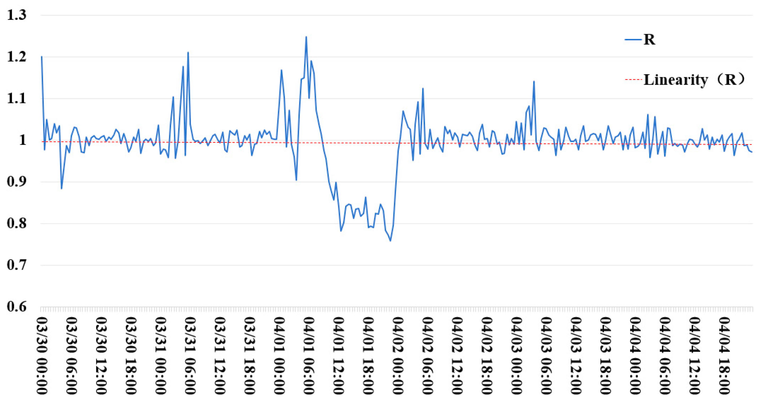
Based on the prediction results and the calculated relative errors, the root mean square error RMSE of urban road network resilience performance changes was further computed according to Equation (6) (with α1 = α2 = α3 = α4 = 0.25), as shown in Figure 6 and Figure 7.
Based on the analysis of the above figure, the disturbance onset time t0 and recovery time t2 of the urban transportation network were determined to be from 10:30 AM to 5:45 PM on 1 April. The composite resilience measurement indicator, R, integrating supply, efficiency, and cost of the urban transportation network was then calculated, as shown in the following Figure 7.
By consulting the weather data for that day, it was found that heavy rainfall began after 9:30 AM on 1 April and gradually returned to normal conditions after 5:30 PM. Comparative analysis with Figure 5 indicates the following: (1) The composite resilience measurement value of the system continuously declined after 10:00 AM on 1 April, reaching a minimum of 0.78 at 18:10, indicating that the system had approximately 30 min of resistance buffering against the heavy rainfall impact. (2) Between 18:10 and 20:15, the system remained in a low-level fluctuating state, and after 20:15, it began to recover rapidly, with a total recovery time of 2 h and 5 min. (3) By 23:30, the system recovered to 0.87, reaching the normal level for the same period.
Thus, the calculated composite resilience curve of the urban transportation network in terms of supply, efficiency, and cost closely matches the actual conditions, achieving minute-level dynamic monitoring of the resilience index.

4. Conclusions

This study employs ride-hailing big data to investigate the resilience characteristics of urban transportation networks. Compared with previous studies based on taxi or bus operational data, this approach offers broader coverage of travel characteristics and a faster evaluation process, enabling fine-grained, minute-level dynamic measurement of urban transportation network resilience, as opposed to the traditional hourly level assessment.
In constructing the urban transportation network resilience assessment model, a transportation cost indicator was introduced to establish a multidimensional resilience measurement system encompassing supply–demand balance, efficiency, and cost. By leveraging the advantages of Long Short-Term Memory (LSTM) networks in handling time-series data, combined with the self-attention mechanism of the Transformer to capture long-term dependencies, the model achieves an average prediction accuracy of 96.8% for resilience indicators, thereby improving the precision and sensitivity of urban transportation network resilience assessment.
The real-time assessment and predictive capabilities of this study have significant practical value. The model can monitor network performance in real time and quickly identify the extent of road network performance degradation as well as the start and end points of critical recovery phases when external disturbances occur. This provides emergency decision-making support for urban traffic management authorities. Additionally, based on the model’s predictive results, management departments can implement emergency response strategies more promptly and effectively, enabling more efficient allocation of resources.
In addition, this study still has room for improvement, particularly regarding the rationality of the weight assignment in the composite resilience indicator expressed in Formula (6). In future work, we will determine more scientifically grounded weights using data-driven optimization methods based on the management objectives and data characteristics of specific cities. We will also further explore the integration of multi-modal transportation data to continuously enhance the practical applicability of the proposed model.

Author Contributions

Conceptualization, Z.Y. and Y.Q.; methodology, N.G. and X.M.; software, N.G. and X.M.; validation, N.G. and X.M.; formal analysis, N.G., X.M. and Z.Y.; data curation, N.G. and X.M.; writing—original draft preparation, N.G. and X.M.; writing—review and editing, N.G. and Z.Y.; visualization, X.M.; supervision, Z.Y. and Y.Q.; project administration, Z.Y. and Y.Q.; funding acquisition, Z.Y. All authors have read and agreed to the published version of the manuscript.

Funding

The work in this paper is supported by The National Key Research and Development Program of China (Grants No. 2022ZD0162200), and the Natural Science Foundation of Jiangsu Province (Grants No. BK20241484).

Data Availability Statement

The data used in this study are available upon request to the corresponding authors.

Acknowledgments

The authors used Deepseek 3.1 to improve the readability of the manuscript.

Conflicts of Interest

The authors declare that there are no conflicts of interest.

References

  1. Du, J.; Ren, G.; Cui, J.; Cao, Q.; Wang, J.; Wu, C.; Zhang, J. Monitoring of operational resilience on urban road network: A Shaoxing case study. Reliab. Eng. Syst. Saf. 2025, 257, 110836. [Google Scholar] [CrossRef]
  2. Zhou, W.; Zhang, X.; Xue, Q.; Shi, C. Hourly-level resilience measurement model for urban transportation networks under emergencies. J. Transp. Eng. Inf. Technol. 2025, 1–18. (In Chinese) [Google Scholar] [CrossRef]
  3. Huang, J.; Hu, G.; Shi, J.; Chen, S. Research on urban transportation system resilience: Conceptions, characteristics, and key issues. City Plan. Rev. 2025, 49, 119–130. (In Chinese) [Google Scholar]
  4. Serdar, M.Z.; Koç, M.; Al-Ghamdi, S.G. Urban transportation networks resilience: Indicators, disturbances, and assessment methods. Sustain. Cities Soc. 2022, 76, 103452. [Google Scholar] [CrossRef]
  5. Rezvani, S.M.H.S.; Silva, M.J.F.; de Almeida, N.M. Urban Resilience Index for Critical Infrastructure: A Scenario-Based Approach to Disaster Risk Reduction in Road Networks. Sustainability 2024, 16, 4143. [Google Scholar] [CrossRef]
  6. Balakrishnan, S.; Jin, L.; Cassottana, B.; Costa, A.; Sansavini, G. Developing resilience pathways for interdependent infrastructure networks. Sustain. Cities Soc. 2024, 115, 105795. [Google Scholar] [CrossRef]
  7. Holling, C.S. Resilience and stability of ecological systems. Annu. Rev. Ecol. Syst. 1973, 4, 1–23. [Google Scholar] [CrossRef]
  8. Pimm, S.L. The complexity and stability of ecosystems. Nature 1984, 307, 321–326. [Google Scholar] [CrossRef]
  9. Zhou, Y.; Wang, J.; Yang, H. Resilience of transportation systems: Concepts and omprehensive review. IEEE Trans. Intell. Transp. Syst. 2019, 20, 4262–4276. [Google Scholar] [CrossRef]
  10. Bruneau, M.; Chang, S.E.; Eguchi, R.T.; Lee, G.C.; O’Rourke, T.D.; Reinhorn, A.M.; Shinozuka, M.; Tierney, K.; Wallace, W.A.; Von Winterfeldt, D. A framework to quantitatively assess and enhance seismic resilience of communities. Earthquake Spectra. 2003, 19, 733–752. [Google Scholar] [CrossRef]
  11. Chen, C.; He, F.; Zhao, D.; Xie, M. A resilience assessment method for urban road public transportation systems based on system function curves. J. Tsinghua Univ. (Sci. Technol.) 2022, 62, 1016–1022. (In Chinese) [Google Scholar]
  12. Huang, J.; Wang, J. Theory, methodology, and empirical study of travel resilience. Acta Geogr. Sin. 2023, 78, 2507–2519. (In Chinese) [Google Scholar]
  13. Li, D.; Zhu, X.; Huang, G.; Feng, H.; Zhu, S.; Li, X. A hybrid method for evaluating the resilience of urban road traffic network under flood disaster: An example of Nanjing, China. Environ. Sci. Pollut. Res. 2022, 29, 46306–46324. [Google Scholar] [CrossRef]
  14. Boeing, G.; Ha, J. Resilient by design: Simulating street network disruptions across every urban area in the world. Transp. Res. Part A Policy Pract. 2024, 182, 104016. [Google Scholar] [CrossRef]
  15. Henke, I.; Troiani, G.; Pagliara, F. An analysis of the vulnerability of road networks in response to disruption events through accessibility indicators specification. Transp. Plan. Technol. 2024, 47, 628–655. [Google Scholar] [CrossRef]
  16. Ferrari, C.; Santagata, M. Vulnerability and robustness of interdependent transport networks in north-western Italy. Eur. Transp. Res. Rev. 2023, 15, 6. [Google Scholar] [CrossRef]
  17. Tang, S.; Zhu, W.; Cheng, G.; Zheng, J.; Zhou, J. Safety resilience assessment of urban road traffic system under rainstorm and waterlogging. China Saf. Sci. J. 2022, 32, 143–150. (In Chinese) [Google Scholar]
  18. Pan, X.; Dang, Y.; Wang, H.; Hong, D.; Li, Y.; Deng, H. Resilience model and recovery strategy of transportation network based on travel OD-grid analysis. Reliab. Eng. Syst. Saf. 2022, 223, 108483. [Google Scholar] [CrossRef]
  19. Bergantino, A.S.; Gardelli, A.; Rotaris, L. Assessing transport network resilience: Empirical insights from real-world data studies. Transp. Rev. 2024, 44, 834–857. [Google Scholar] [CrossRef]
  20. Postorino, M.N.; Sarnè, G.M.L. A New Approach to Assessing Transport Network Resilience. Urban Sci. 2025, 9, 35. [Google Scholar] [CrossRef]
  21. Zhang, G.; He, C.; Zhang, J.; Zhai, Y.; Zhang, Z.; Jiang, L.Z.; Guo, W. Prediction of Bridge Structure Response and Resilience Assessment Under Main-Aftershock: LSTM-Transformer Model Based on Adaptive Learning Rate Framework. Eng. Struct. 2025, 345, 121449. [Google Scholar] [CrossRef]
  22. Han, L.; Abdel-Aty, M.; Yu, R.; Wang, C. LSTM + Transformer Real-Time Crash Risk Evaluation Using Traffic Flow and Risky Driving Behavior Data. IEEE Trans. Intell. Transp. Syst. 2024, 25, 18383–18395. [Google Scholar] [CrossRef]
  23. Yao, Z.; Liu, C. Research on the fusion application of LSTM and transformer in network traffic prediction. In Proceedings of the International Conference on Artificial Intelligence and Machine Learning Research (CAIMLR 2024), Singapore, 28–29 September 2024; Volume 13635, pp. 72–78. [Google Scholar]
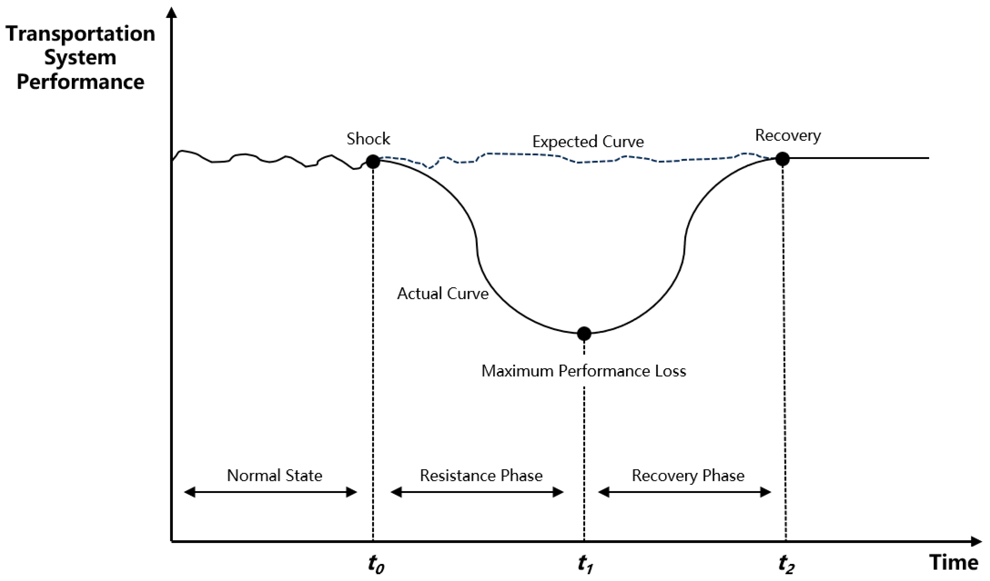
Figure 1. Urban Transportation Network System Resilience Performance Curve.
Electronics 15 00002 g001
Figure 2. Framework of the Expected Resilience Curve Prediction Algorithm Based on LSTM-Transformer.
Electronics 15 00002 g002
Figure 3. Time-Varying Diagrams of Ride-Hailing Travel Data in a Certain City During a Specific Period.
Electronics 15 00002 g003aElectronics 15 00002 g003b
Figure 4. Predicted Curves of Ride-Hailing Travel Data Based on LSTM-Transformer.
Electronics 15 00002 g004
Figure 5. Relative Prediction Error Curves of Ride-Hailing Travel Data Based on LSTM-Transformer.
Electronics 15 00002 g005
Figure 6. Comprehensive Relative Error (RMSE) Curve of Ride-Hailing Travel Data Predictions Based on LSTM-Transformer.
Electronics 15 00002 g006
Figure 7. Composite Resilience Curve of Urban Transportation Network Integrating Supply, Efficiency, and Cost.
Electronics 15 00002 g007
Disclaimer/Publisher’s Note: The statements, opinions and data contained in all publications are solely those of the individual author(s) and contributor(s) and not of MDPI and/or the editor(s). MDPI and/or the editor(s) disclaim responsibility for any injury to people or property resulting from any ideas, methods, instructions or products referred to in the content.