CiTranGAN: Channel-Independent Based-Anomaly Detection for Multivariate Time Series Data

Abstract

Anomaly detection, as a critical task in time series data analysis, plays a pivotal role in ensuring industrial production safety, enhancing the precision of climate predictions and improving early warning for ocean disaster. However, due to the high dimensionality, redundancy, and non-stationarity inherent in time series data, rapidly and accurately identifying anomalies presents a significant challenge. This paper proposes a novel model CiTranGAN, which integrates the advantages of Transformer architecture, generative adversarial networks, and channel-independence strategies. In this model, the channel-independent strategy eliminates cross-channel interference and mitigates distribution drift in high-dimensional data. To mitigate redundancy and enhance multi-scale temporal feature representation, we constructed a feature extraction module that integrates downsampling, convolution, and interaction learning. To overcome the limitations of the traditional attention mechanism in detecting local trend variations, a hybrid dilated causal convolution-based multi-scale self-attention mechanism is proposed. Finally, experiments were conducted on five real-world multivariate time series datasets. Compared with the baseline models, CiTranGAN achieves average improvements of 12.48% in F1-score and 7.89% in AUC. In the ablation studies, CiTranGAN outperformed the channel-independent mechanism, the downsampling–convolution–interaction learning module, and the multi-scale convolutional self-attention mechanism, with respective average increases in AUC of 1.63%, 2.16%, and 3.47%, and corresponding average improvements in F1-score of 1.70%, 4.33%, and 2.04%, respectively. These experimental results demonstrate the rationality and effectiveness of the proposed model.

1. Introduction

With the continuous development of technologies such as the Internet of Things and sensors, a large amount of time series data have been generated across various domains, including industrial production, medical diagnostics, and smart ocean systems [1,2]. However, due to the intrinsic complexity and diversity of domain-specific backgrounds, as well as the influence of both objective environmental and subjective human factors, various types of anomalies may be hidden in the data collected by sensors.

An anomaly generally denotes data patterns that deviate from normal or expected behavior [3]. These can be categorized into three types: point anomalies, context anomalies, and collective anomalies [4]. Among these, collective anomalies present the greatest detection challenge. In such cases, individual data points may not exhibit anomalous behavior independently; however, when they occur in a specific combination, they manifest as anomalies. The presence of such anomalies can negatively impact production efficiency, product quality, and workplace safety [5], and they can also influence leadership decision making. Therefore, the timely identification and rectification of anomalies is a critical task [6].

In time series data, anomaly detection methods can be categorized based on the number of variables involved. The simplest category is univariate anomaly detection, which involves analyzing time series data from a single sensor to identify anomalies from normal patterns. However, in practical applications, multiple sensors operate concurrently, generating multivariate time series (referred to as MvTS). These datasets may exhibit intricate variable correlations and temporal dependencies, with anomalies that may evolve significantly over time. Moreover, as the sampling frequency increases and the data length grows, the task of multivariate anomaly detection becomes more challenging [7].

With the substantial advancements in deep learning technologies, particularly in terms of scale and computational efficiency, deep neural networks have exhibited excellent performance in multivariate anomaly detection tasks across various domains [8]. For example, LSTM-NDT [9] integrates the Long Short-Term Memory model with a dynamic threshold estimation method to detect anomalies in time series data by analyzing prediction errors. USAD [10] embeds adversarial training strategies into unsupervised autoencoders, effectively addressing common challenges such as mode collapse and non-convergence in traditional GANs. TranAD [11] utilizes the self-attention mechanism in Transformer to capture temporal relationships within MvTS data and detects anomalies by reconstruction errors. This method has exhibited superior performance across diverse datasets. However, existing studies have not adequately addressed key characteristics such as temporal redundancy, local trend variation, and long-term dependencies in the data, as shown in Figure 1. These unaddressed aspects impact the accuracy of anomaly detection in MvTS data.

In MvTS analysis, Transformer-based methods generally adopt a channel-dependent strategy to capture inter-variable correlations. These methods assume that all the time series in the set come from the same process and fit a single univariate function [12]. However, real-world datasets often originate from diverse sources, such as IoT sensors, user behavior logs, and environmental monitors. These variables (or channels) may have varying scales, units, or noise levels, and their relationships may also be nonlinear or spurious correlations. For example, in climate modeling, temperature and humidity might appear correlated due to seasonal trends, but their relationship can break down during extreme weather events. In this case, the model trained on historical data would fail during anomalies. Fortunately, recent advancements have led to the emergence of methods that employ the channel-independent strategy [13]. These methods view multivariate time series data as separate univariate time series and disregard the correlation between channels. Existing research shows that channel-independent methods have a high capacity and low robustness, while the channel-dependent method has a low capacity and high robustness. In real-world, non-stationary time series, where factors such as noise and distribution drift are prevalent, robustness becomes more critical. This explains why channel-independent methods generally outperform in most practical scenarios.

To address the above challenges, we propose a novel multivariate time series anomaly detection model named CiTranGAN (channel-independent, Transformer-based, and generative adversarial network). This model introduces a channel-independence strategy to mitigate the interdependencies among feature variables and address data distribution drift. It employs data decomposition techniques to reduce redundancy and convolutional interactions to enhance information exchange and collaborative learning across different temporal scales. Additionally, a multi-scale convolution self-attention mechanism is utilized to capture both local and long-term dependencies within the data. Consequently, the proposed method aims to enhance the reliability and accuracy of anomaly detection for MvTS data. The main contributions of this paper are as follows:

• A novel multivariate time series anomaly detection model CiTranGAN is proposed, which integrates the advantages of Transformer architecture, generative adversarial networks, and channel-independence strategies.
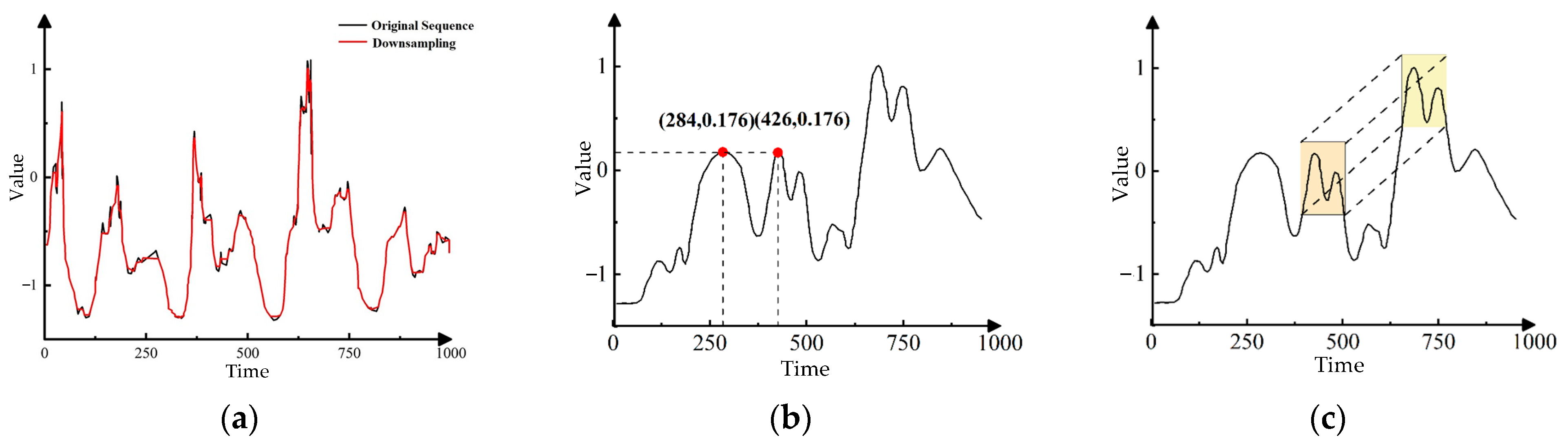
• Temporal feature extraction leveraging downsampling–convolution–interaction learning. Specifically, downsampling serves to reduce redundancy while also enhancing the extraction of long-term trend features. One-dimensional convolution effectively identifies local patterns and detailed features. The interaction operation iterates over different time resolutions, promoting efficient information exchange. This enhances the visibility of features across varying time scales, ultimately improving model performance. This process ultimately leads to an enhancement in the overall performance of the model.
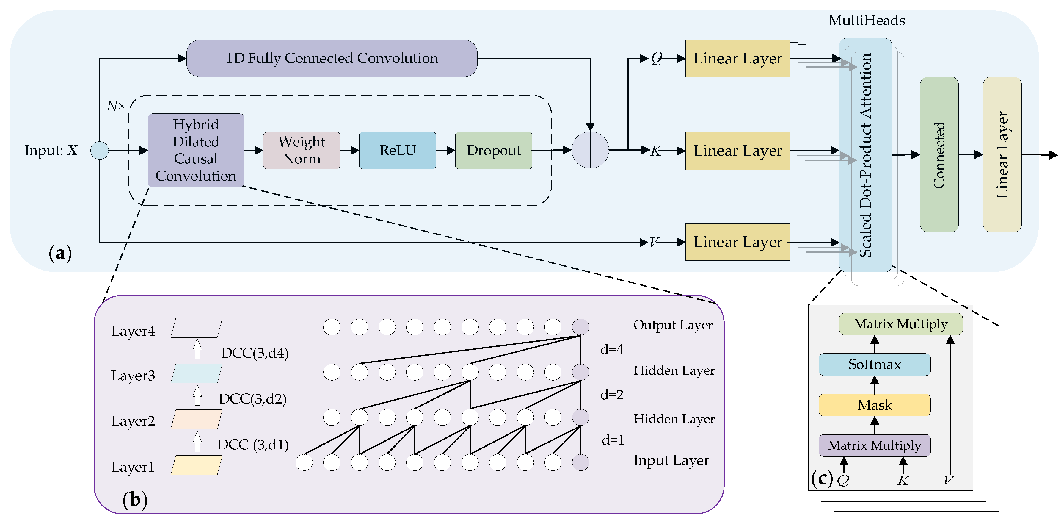
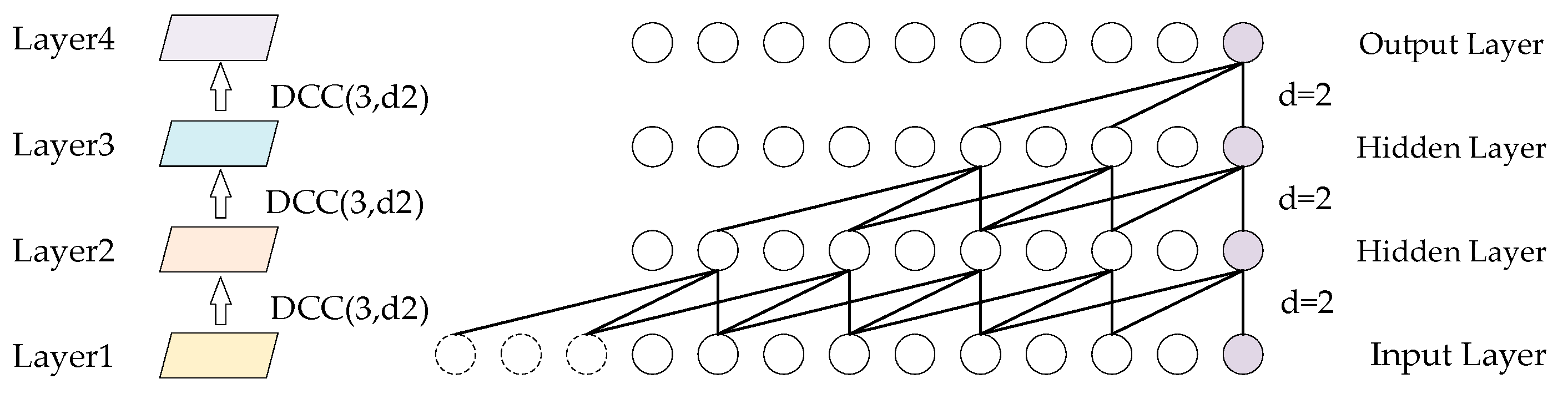
• A multi-scale convolutional self-attention mechanism is designed based on hybrid dilated causal convolutions, which overcomes the limitations of the traditional self-attention mechanism in identifying the local variation trend within subsequences. Specifically, causal convolutions ensure that the model relies only on input features from prior time points, thereby preventing future information leakage. Dilated convolutions expand the receptive field of the model, enabling it to effectively capture nonlinear relationships within long sequences. Additionally, dilation factors are dynamically allocated at different layers according to practical requirements, further enhancing the ability to capture contextual information across varying time scales. By integrating these advantages, the model is better capable of emphasizing the influence between similar subsequences.

2. Related Work

In practical applications and research involving MvTS data, the scarcity of labeled data and the diversity of anomalies necessitate the use of unsupervised learning methods for anomaly detection. Initially, traditional algorithms such as clustering [14,15], principal component analysis [16,17], and autoregressive [18,19] were predominantly utilized. These methods detect anomalies through modeling and feature extraction from time series data. However, they exhibit limitations when handling complex nonlinear features [20]. Recently, deep learning technologies have demonstrated significant potential in addressing these challenges [21], particularly in representing intricate relationships and high-dimensional data. Anomaly detection methods based on deep learning are mainly divided into two categories: prediction-based method and reconstruction-based method.

In prediction-based methods, recurrent neural networks and their variants [22,23,24,25] are predominantly utilized. These models effectively capture long-term dependencies and sequence patterns by constructing predictive models. For example, LSTM-NDT [9] identifies anomalies through the prediction errors from an LSTM model and introduces a parameter-free dynamic threshold estimation method, offering a novel solution for anomaly detection in multivariate data. However, these methods primarily depend on historical data for predictions. In practical applications, the uncertainty of future data can lead to a decline in prediction accuracy, particularly when dealing with rapidly changing or high-dimensional data. Additionally, their computational complexity presents a significant challenge [26].

In reconstruction-based methods, autoencoders [27,28,29] can be utilized to train on normal data. Specifically, the encoder compresses the input data into a low-dimensional latent representation, while the decoder reconstructs the data from this latent space, thereby capturing the intrinsic features and patterns of normal data. Additionally, GANs [10,30] can also be employed for training purposes. In this context, the generator synthesizes time series data, whereas the discriminator evaluates whether the data are real or generated. In recent years, Transformer architecture [31] has gained significant attention for its exceptional capability to handle complex relationships in time series data. Anomaly detection models based on self-attention mechanisms [11,32] effectively capture dependencies among time steps within sequences, quantify deviations from normal patterns by assessing association differences, and evaluate anomalies via reconstruction error. These models have exhibited superior performance across a variety of datasets.

In summary, deep learning technology has brought new vitality into the anomaly detection task for MvTS data. However, existing studies frequently overlook the intrinsic characteristics and local trend variations, which can reduce the accuracy of anomaly detection. In the face of practical challenges, these methods still prove to be inadequate.

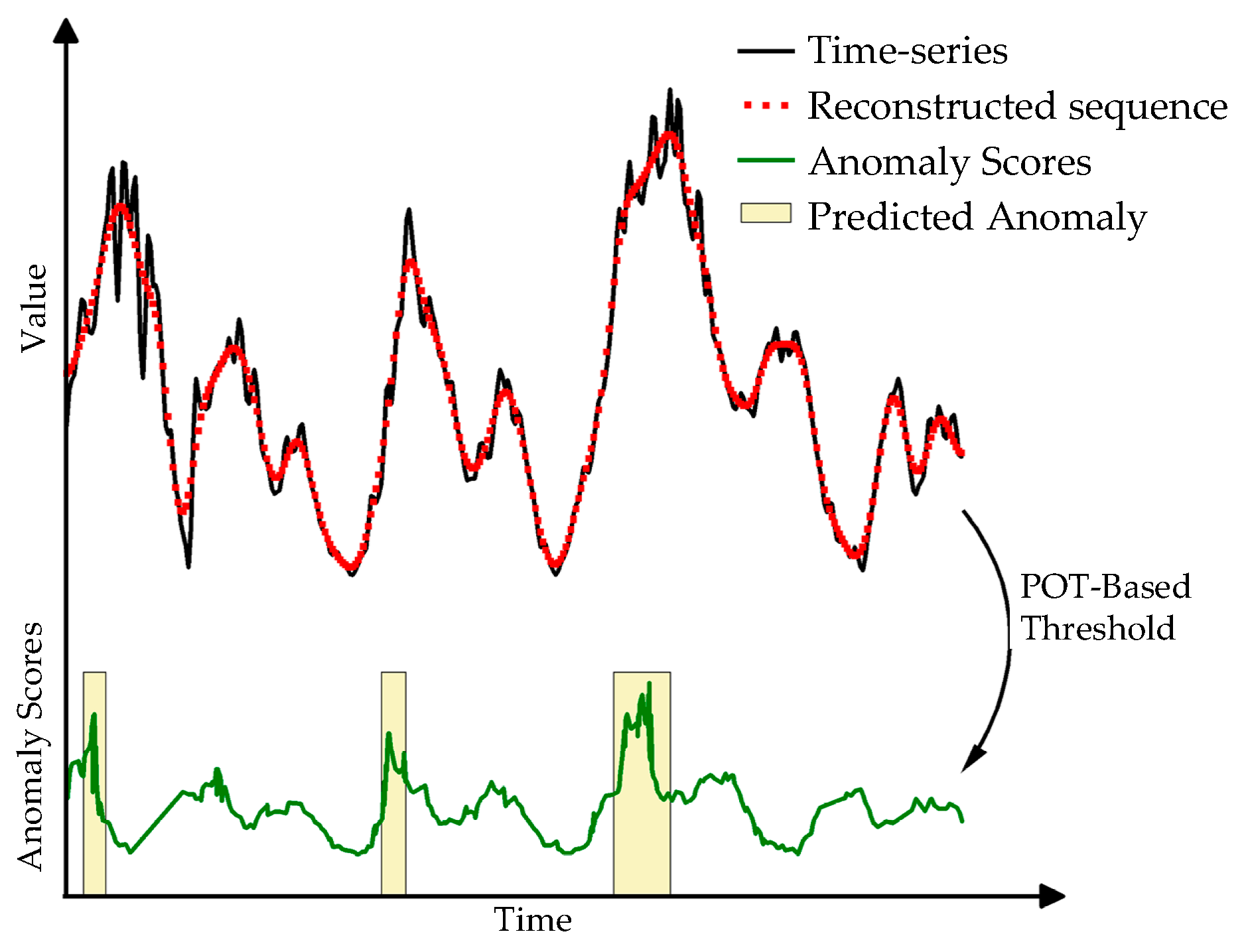
3. Anomaly Detection for Multivariate Time Series Data

3.1. Preliminaries

Time series data [33] are typically denoted as $\mathit{X}=\{x_1,...{,x}_t,...,x_T\}$. Where $x_t\in R^M$ represents the observed values of M variables (or channels) collected at each time step t. When M ≥ 2, $\mathit{X}$ represents the MvTS data. T represents the total time length. The intervals between consecutive time points t − 1, t and t + 1 are equidistant [34].

In practical applications, various feature variables within $\mathit{X}$ may have distinct units of measurement. To address the issue of uneven weight distribution among features in the model, a maximum–minimum normalization technique is commonly employed to standardize the data, as shown in Equation (1):

$$x\prime ={\displaystyle \frac{x-\mathit{min}(\mathit{X})}{\mathit{max}(\mathit{X})-\mathit{min}(\mathit{X})}}.$$

(1)

Simultaneously, to address the issue of traditional models experiencing a significant decline in performance as the input sequence length increases, the sliding window technique [35] is employed. This technique segments long sequences into multiple shorter ones, processing the data in batches within each window. Specifically, the input data $\mathit{X}$ are transformed into a series of sliding windows $\mathit{W}=\{W_1,...,W_l,...,W_L\}$. Here,$W_l=\{x_{t-K+1},...,x_t\}$ denotes the context window of length K at time t. When t < K, a constant vector $\{x_t,...,x_t\}$ is appended to the window, ensuring that each window maintains a consistent length K.

In the anomaly detection task for MvTS data [36], given a dataset, $\mathit{X}$, the model utilizes the window sequence $\mathit{W}$ as the training data. First, the unseen test data $\widehat{\mathit{X}}$ are constructed as a sliding window sequence $\widehat{\mathit{W}}$, which subsequently reconstructs the input window $\widehat{\mathit{W}}$. The anomaly score s of the input data is determined based on the deviation between the input window and its reconstructed vector (See Section 3.2.4 for details). The Peaks Over Threshold (POT) method [11] is employed to dynamically generate the threshold. If the anomaly score exceeds this threshold, the corresponding time-stamp is flagged as an anomaly. Finally, it predicts labels for the entire test dataset $\widehat{\mathit{X}}$, resulting in a label set $y=\{y_1,...,y_t,...y_{\widehat{T}}\}$, where each $y_t$ ∈ {0,1}. Specifically, $y_t$ = 1 indicates that the data point at time t is abnormal, as shown in Figure 2.

The POT specifically models anomalies that exceed an initial threshold, i.e., the tail values, based on Extreme Value Theory (EVT). This enables an accurate characterization of the data’s statistical properties, particularly long-tail behavior, and facilitates adaptive thresholding. Notably, POT requires no prior assumptions about the underlying data distribution and operates without manual intervention. When combined with window normalization techniques, it can automatically adjust thresholds to account for distributional shifts across different data domains. This method not only addresses the challenge of cross-domain generalization but also maintains a low computational complexity of O(N), making it widely applicable to anomaly detection tasks.

The POT is a threshold determination technique that works by dynamically fitting a Generalized Pareto Distribution (GPD) [37] in real time, as shown in Equation (2):

$${\overline{H}}_{th}=P(\mathit{X}-th>x|\mathit{X}>th)~(1+{\displaystyle \frac{\gamma x}{\sigma }}{)}^{-{\displaystyle \frac{1}{\gamma }}}.$$

(2)

Here, ${\overline{H}}_{th}$ represents the cumulative distribution function of $x$ conditioned on values exceeding a predefined threshold; $\gamma$ and $\sigma$ correspond to the shape and scale parameters of the fitted GPD, respectively. $th$ refers to the initial threshold, which is typically determined through statistical methods such as the quantile method. $\mathit{X}-th$ represents the amount by which a value exceeds the threshold.

The parameters in the GPD are typically estimated through the Maximum Likelihood Estimation [38], as shown in Equation (3):

$$\widehat{\theta }=\mathit{arg}\underset{\theta }{\mathit{max}}{\prod }_{i-1}^n[1-\mathit{exp}\{-(1+{\displaystyle \frac{\gamma x}{\sigma }}\left)\right\}].$$

(3)

Here, $n$ represents the number of observation points, and $\theta$ represents the set of GPD parameters. The goal is to find the parameter values that maximize the likelihood of the observed extreme data conforming to the GPD.

The calculation method for the threshold $t{h}_f$ is shown in Equation (4):

$$t{h}_f\simeq th-{\displaystyle \frac{\widehat{\sigma }}{\widehat{\gamma }}}\left(\right({\displaystyle \frac{qn}{P}}{)}^{-\widehat{\gamma }}-1).$$

(4)

Here, $th$ represents the initial threshold, $q$ represents the proportion of values exceeding the threshold, $\widehat{\gamma }$ and $\widehat{\sigma }$ are the estimated value of the shape and scale parameters of GPD, respectively, and $P$ represents the number of values that exceed the threshold.

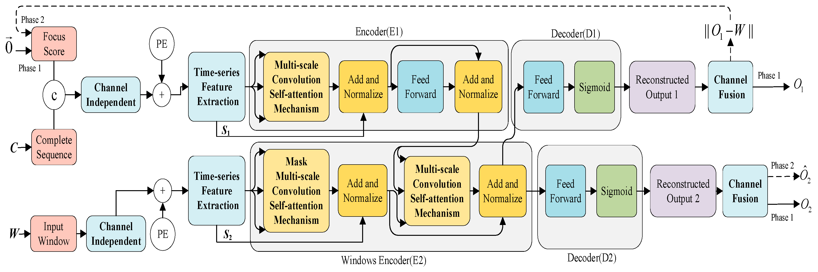
3.2. CiTranGAN

The objective of anomaly detection is to accurately and efficiently identify anomalies. Consequently, a novel multivariate time series anomaly detection model, CiTranGAN, was constructed, which integrates a channel-independent strategy Transformer-based architecture with a generative adversarial network. The overall framework is shown in Figure 3.

This model comprises two encoders and two decoders. To mitigate the issue of distribution drift in the raw observational data, it implements three critical preprocessing operations: channel independence, normalization, and positional encoding. The preprocessed data are subsequently fed into the temporal feature extraction module, which alleviates temporal redundancy by collaboratively learning features across various time scales. The resultant vector representation of feature variables serves as input to the encoder. Within the encoder, a multi-scale convolutional self-attention mechanism is established to augment the interaction between similar time subsequences.

In E1, the complete sequence is transformed into a low-dimensional vector representation. In E2, by employing the sliding window method, the encoding of the input window is generated based on the vector representation obtained from E1. The decoder, through reverse operations, converts this generated encoding into a reconstruction sequence that closely mirrors the original input data, subsequently concatenating it to restore its initial multivariate structure. Finally, the anomaly is determined based on the anomaly score. In this model, the normalization, positional encoding, and feed-forward neural network structures are consistent with those in the original Transformer architecture and therefore will not be discussed in detail here. In the following sections, we provide an in-depth examination of the functions and principles of the primary enhanced modules.

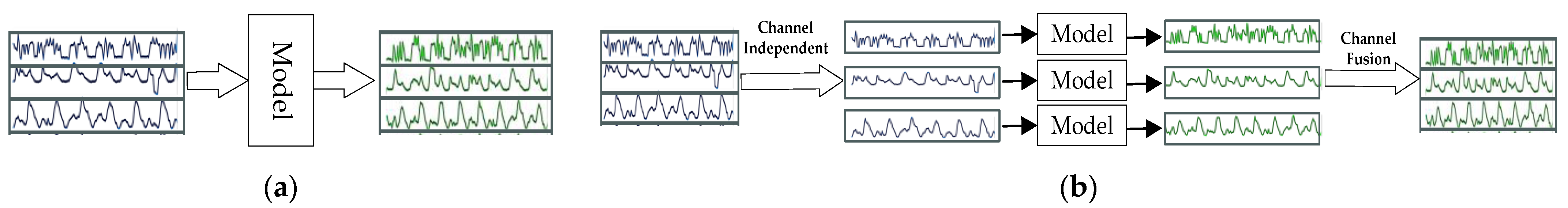
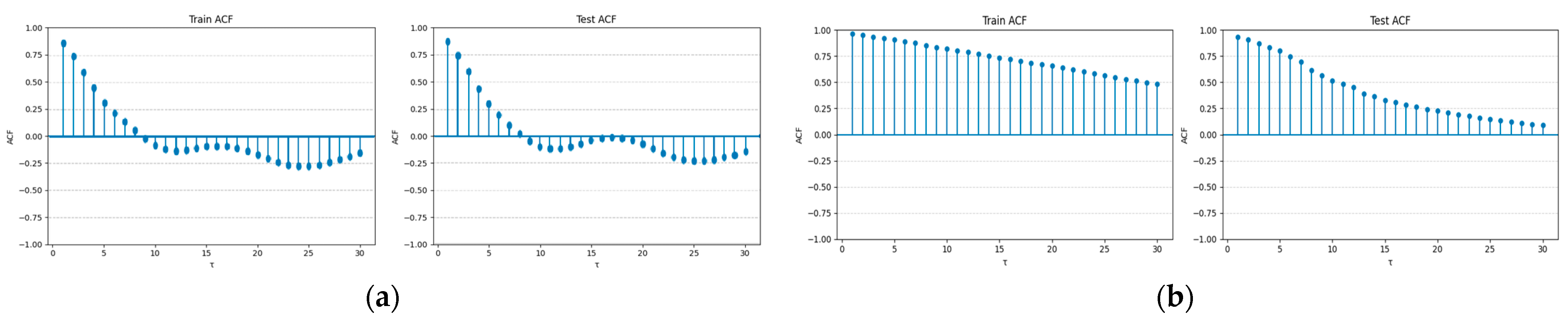
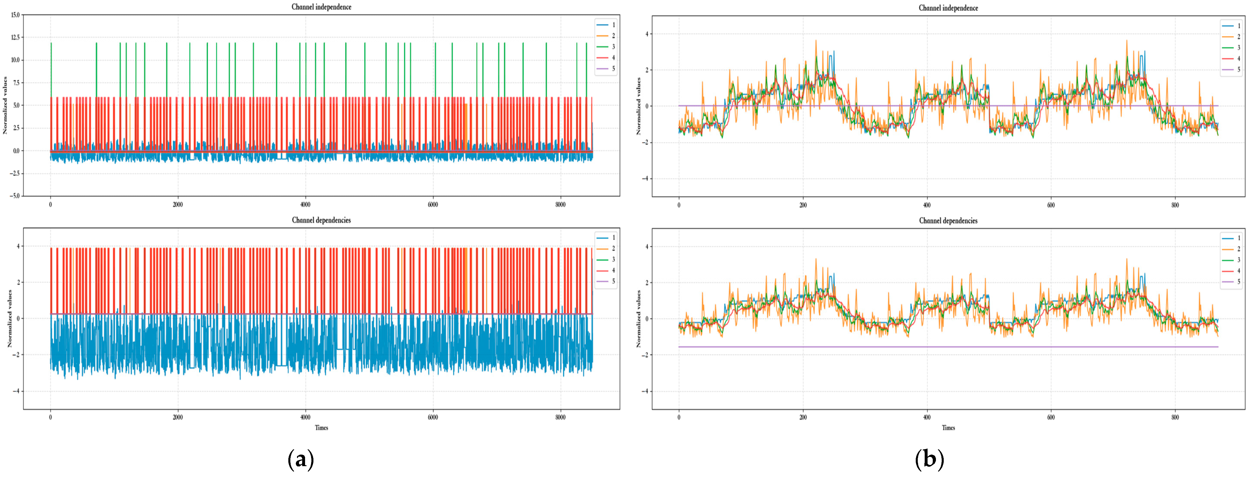
3.2.1. Channel-Independent Module

In the MvTS analysis task, the channel-dependent (CD) strategy is commonly employed within traditional Transformer architectures. We can see from Figure 4a that the CD strategy takes all the variables (channels) as a whole input and aims to capture the interrelationships among them. Specifically, the data are directly integrated into a single vector and subsequently mapped into the embedding space. Here, the objective of CD is minimizing the loss of different variables, as shown in Equation (5):

$$\underset{f}{min}{\displaystyle \frac{1}{T}}{\sum }_{i=1}^T\mathcal{l}\left(f\right({\mathit{X}}^{\left(i\right)},{\mathit{Y}}^{\left(i\right)}\left)\right).$$

(5)

where $\mathcal{l}$ is the reconstruction loss, and $T$ is the number of time-stamps used for training.

However, real-world data evolve over time and are often subject to shifts or drifts in data distribution. As shown in Figure 5, the autocorrelation function (ACF) [39] of the SMAP and SWaT dataset reveals statistically significant differences between the training and testing phases. Since the effectiveness of the model heavily relies on the assumption that the data originate from the same independent distribution, the distribution drift poses a considerable challenge and significantly affects the accuracy of data reconstruction. To mitigate the impact of data distribution drift, reduce the interactions among variables, and enhance the model’s robustness, a channel-independent (CI) strategy is employed in constructing the anomaly detection model.

The CI strategy treats the multiple variables as a set of independent univariate time series, as shown in Figure 4b. Specifically, each variable is processed as a separate channel, although all channels share the same backbone model. Notably, the forward propagation process for each channel remains independent. Upon the completion of training, the reconstructed outputs from each channel are concatenated to restore the original multivariate structure. The reconstruction loss for the CI strategy is calculated as the average of all individual channel losses, as shown in Equation (6):

$$\underset{f}{min}{\displaystyle \frac{1}{TM}}{\sum }_{i=1}^T{\sum }_{m=1}^M\mathcal{l}\left(f\right(x_m^{\left(i\right)},y_m^{\left(i\right)}\left)\right),$$

(6)

where $T$ is the number of time-stamps, and M is the number of variables (or channels); $\mathcal{l}$ is the reconstruction loss, which is minimized independently for each channel.

Based on Equations (5) and (6), for the detection of anomaly MvTS data, the CD strategy primarily depends on the average of the ACF across all channels, whereas the CI strategy requires considering the ACF for each individual channel separately. Since the drift in the average ACF is generally smaller than the drift in the ACF of a single channel, it can be concluded that the CI strategy demonstrates superior performance.

Meanwhile, we selected the first five variables from the SMAP and SWaT datasets, and those variables were standardized using both the CI and CD, as shown in Figure 6. The CI strategy proves more effective in preserving the intrinsic characteristics of the original variables, whereas the CD strategy tends to either excessively compress or amplify these features. We can see from Figure 5 and Figure 6 that for the SMAP dataset, although the distribution shift is relatively small, the CD strategy has a substantial impact on normalization; in contrast, the opposite is observed for the SWaT dataset. This contrast is particularly pronounced when dealing with real-world datasets, as CD models might force a false dependency between these channels, leading to biases. Furthermore, compared with CD, the CI strategy offers significant advantages in terms of robustness, applicability, and computational complexity. Therefore, we adopt the CI strategy in constructing the anomaly detection model.

3.2.2. Temporal Feature Extraction Module

As the sampling frequency increases, the data collected in practical applications may contain significant redundant information, as shown in Figure 1a. For instance, when MvTS is represented as a matrix $\mathit{X}$ ∈ R^M×T, it is frequently observed that rank($\mathit{X}$) < min(M, T). This indicates that $\mathit{X}$ possesses low-rank properties and contains temporal redundancy. Moreover, due to variations in the number of sensors, the data will exhibit different characteristics depending on the time and scene conditions. Therefore, the key challenge is to effectively capture temporal features from MvTS data that contain such redundancies.

After downsampling the original data, the downsampled sequence maintains a high degree of similarity with the original sequence in terms of temporal relationships, including trends and seasonal components, as shown in Figure 1a. It is evident that the time series data exhibit consistent features across various time frequencies. Moreover, a reduced yet independent dataset can effectively capture the essential characteristics of the complete dataset. Based on these observations, a downsampling–convolution–interactive learning module structure is proposed, as shown in Figure 7.

As shown in Figure 7a, the input data $\mathit{X}$ are separated into odd and even subsequences through downsampling, denoted as ${\mathit{X}}_{odd}$ and ${\mathit{X}}_{even}$, respectively. To enhance the model’s feature extraction capability and mitigate potential information loss during the downsampling process, a novel interactive learning strategy is proposed.

In this strategy, ${\mathit{X}}_{odd}^N$ and ${\mathit{X}}_{even}^N$ are independently fed into two one-dimensional (1D) convolution modules, α and β, producing α(${\mathit{X}}_{odd}^N$) and β(${\mathit{X}}_{even}^N$). These representations are then fused with ${\mathit{X}}_{odd}^N$ and ${\mathit{X}}_{even}^N$ via element-wise operations, allowing bidirectional information exchange between the two subsequences. The resulting updated sequences are denoted as ${\mathit{X}\prime }_{odd}$ and ${\mathit{X}\prime }_{even}$, as shown in Equations (7) and (8):

$${\mathit{X}\prime }_{odd}={\mathit{X}}_{odd}^N\odot \mathit{exp}(\alpha \left({\mathit{X}}_{even}^N\right)),$$

(7)

$${\mathit{X}\prime }_{even}={\mathit{X}}_{even}^N\odot \mathit{exp}(\beta \left({\mathit{X}}_{odd}^N\right)).$$

(8)

Here, exp represents an exponential function, and $\odot$ denotes a dot product operation. α and β represent 1D convolution modules, as shown in Figure 7b.

To ensure coordination and consistency in the processing of ${\mathit{X}}_{odd}^N$ and ${\mathit{X}}_{even}^N$, α and β share an identical network structure. In the lD convolution module, the sequence is first padded to address boundary contraction issues. Next, a convolution kernel of size k is utilized to expand the input channel dimension from K to h × K, where h represents the scaling factor of the hidden layer size. Subsequently, LeakyReLU and Dropout are employed to mitigate the vanishing gradient problem and preserve network sparsity. Subsequently, the expanded channel dimension h × K is reduced back to K, effectively performing an inverse mapping of the input data. Finally, the Tanh activation function is used to compress the output features into the range of [−1, 1], ensuring a balanced distribution of positive and negative features and providing a stable numerical range for subsequent calculations. This procedure can be understood as a scaling transformation applied to ${\mathit{X}}_{odd}^N$ and ${\mathit{X}}_{even}^N$, where the scaling factors are adaptively learned through the neural network module.

To further eliminate the redundant effects, a temporal dependency extractor is constructed based on the MLP, as shown in Figure 7c. This module consists of two fully connected layers, a GeLU activation function, and a Dropout layer. It effectively captures the nonlinear features within ${\mathit{X}\prime }_{odd}$ and ${\mathit{X}\prime }_{even}$, while simultaneously reducing redundant dependencies. Then, a residual connection [40] is employed, generating enhanced sequences with improved predictability, denoted as ${\widehat{\mathit{X}\prime }}_{odd}$ and ${\widehat{\mathit{X}\prime }}_{even}$, as shown in Equations (9) and (10):

$${\widehat{\mathit{X}\prime }}_{odd}=\sigma \left({{\mathit{X}}^{\prime }}_{odd}\cdot {\mathit{W}}_{11}^T+b_{11}\right)\cdot {\mathit{W}}_{12}^T+b_{12}+{\mathit{X}\prime }_{odd},$$

(9)

$${\widehat{\mathit{X}\prime }}_{even}=\sigma \left({{\mathit{X}}^{\prime }}_{even}\cdot {\mathit{W}}_{21}^T+b_{21}\right)\cdot {\mathit{W}}_{22}^T+b_{22}+{\mathit{X}\prime }_{even}.$$

(10)

where ${\mathit{W}}_{\mathit{*}}^{\mathit{T}}$ represents the weight matrix, $b_{*}$ represents the bias term, and $\sigma$ represents the GeLU activation function.

In summary, the temporal feature extraction module integrates both local and global information derived from the two downsampled subsequences. By employing the odd–even splitting operation, the feature elements within the subsequences are efficiently reorganized. Finally, the newly generated concatenated sequence $\mathit{X}\prime ={\widehat{\mathit{X}\prime }}_{odd}+{\widehat{\mathit{X}\prime }}_{even}$ serves as the inputs ${\mathit{S}}_1$ and ${\mathit{S}}_2$ for E1 and E2, respectively.

3.2.3. Multi-Scale Convolutional Self-Attention Mechanism

The multi-head self-attention mechanism, as the core component of the Transformer architecture, is shown in Figure 8c. By concurrently executing multiple independent self-attention operations, this mechanism significantly enhances the model’s capacity to capture intricate features. The computational process is detailed in Equation (11):

$$\mathrm{MultiHeadAtt}\left(\mathit{Q},\mathit{K},\mathit{V}\right)=\mathrm{Concat}\left({\mathit{H}}_1,\dots ,{\mathit{H}}_h\right), \mathrm{where} {\mathit{H}}_i=\mathrm{Attention}\left({\mathit{Q}}_i,{\mathit{K}}_i,{\mathit{V}}_i\right)=\mathrm{softmax}\left({\displaystyle \frac{{\mathit{Q}}_i{{\mathit{K}}_i}^T}{\sqrt{d_k}}}\right){\mathit{V}}_i.$$

(11)

where $\mathit{Q}$ represents the query vector, $\mathit{K}$ represents the key vector, $\mathit{V}$ represents the value vector, and $d_k$ represents dimensionality of these vectors.

In the current self-attention mechanism, the similarity between $\mathit{Q}$ and $\mathit{K}$ is computed by considering only the dependencies between the current point and its immediate neighbors. However, this method overlooks the local trend variations within time series data. As a result, the model’s performance is diminished in anomaly detection. Specifically, when two data points have identical absolute values, as shown in Figure 1b, their computed results may exhibit a high degree of similarity. Despite these points having distinct contextual information and individual variation trends, existing models fail to discern whether a given point is an anomaly. Consequently, it is crucial to comprehensively incorporate the contextual information of data points to enhance the model’s capability in capturing local variations and long-sequence features, which is essential for effective anomaly detection.

Based on the multi-head self-attention model, a novel multi-scale convolutional self-attention mechanism is proposed. This mechanism integrates one-dimensional convolution, causal convolution, and dilated convolution, as shown in Figure 8.

To capture local features in time series data, a one-dimensional fully connected convolution structure is introduced prior to the calculation of the attention matrix. To ensure that the output of each hidden layer has the same length as the input data, zero-padding of length k − 1 is applied to each sublayer. Then, a convolutional kernel with step 1 and size k is utilized to transform the padded input into the query $\mathit{Q}$ and $\mathit{K}$ representations, thereby minimizing the matching error between $\mathit{Q}$ and $\mathit{K}$.

To capture long-term historical information, a multi-layer hybrid dilated causal convolution (HDCC) is designed, as shown in Figure 8b. Causal convolution ensures that the model only relies on input features from previous time points, thereby preventing the leakage of future information, which aligns with the processing requirements of time series data. However, its ability for historical dependencies is limited to a linear scale. To address this limitation, dilated convolution (also known as expansion convolution) is employed, which effectively expands the model’s receptive field by introducing a dilation parameter into the convolutional kernel. This architecture not only avoids increasing the parameter complexity but also captures longer-term nonlinear relationships.

However, dilated convolutions are also susceptible to the gridding effect problem. As shown in Figure 9, when the convolution kernel size $k=$ 3 and $d=$ [2, 2, 2] (the dilation factor is 2 in each layer), the information is captured at discrete intervals. This leads to a significant loss of information. Furthermore, as the dilation factor increases in deeper layers, downsampling results in increasingly sparse input samples, which may negatively impact the learning performance. Specifically, information from distant regions may become less relevant to the current task. On the other hand, the information received at the time points in the d-region of layer l may originate from different grid locations, potentially disrupting the consistency of local information. To address this issue and prevent edge loss, as well as to ensure that the receptive field fully covers the region preceding the current time point, HDCC facilitates effective inter-layer information transfer by dynamically adjusting the dilation factor and kernel size.

Assuming there are n convolution layers with convolution kernel size k and expansion factors $[d_1,...,d_i,...,d_n]$, the maximum distance between two non-zero values is defined and utilized as a critical parameter to optimize the configuration of the convolution layer, as shown in Equation (12):

$$M_i=\max [M_{i+1}-2d_i,M_{i+1}-2(M_{i+1}-d_i),d_i].$$

(12)

where $M_n=d_n$, and the design objective is to ensure that $M_2\le k$. As shown in Figure 8b, for $k=$ 3, if the dilation factors are $d=$ [1, 2, 4], then $M_2$ equals 2, satisfying $M_2\le k$. It is evident that HDCC dynamically adjusts the dilation factor size based on the layer number and the required receptive field. This method not only guarantees the effective capture of context information at multiple scales across various convolutional layers but also mitigates information loss due to the grid effect.

Furthermore, existing research has demonstrated that a multi-layer processing mechanism facilitates the progressive learning and extraction of abstract feature representations from input data [41]. However, as the network depth increases, issues such as gradient explosion or gradient vanishing become more pronounced. To address this challenge, inspired by the gating mechanism in LSTM, a residual connection strategy is employed to ensure that the network maintains optimal performance as its depth increases. Specifically, after the data pass through the mixed dilated causal convolution unit, their processing follows the formulation presented in Equation (13):

$$h=\mathit{Activation}(x+{\sum }_{i=0}^{k-1}f\left(i\right)\cdot x_{s-d\cdot i}).$$

(13)

where $k$ represents the convolution kernel size, $d$ represents the expansion factor, and $s-d\cdot i$ represents the subscript of the historical value.

In summary, by utilizing a combination of various convolution operations, the attention mechanism is able to focus more precisely on the temporal subsequences. This not only enhances the interaction among similar temporal subsequences but also effectively mitigates the loss of temporal feature granularity during processing. And the model’s capability to capture local temporal information is significantly improved.

3.2.4. Autoregressive Reasoning and Adversarial Training Module

Similarly to the Transformer architecture, the attention weights are generated through E1, as shown in Equations (14) and (15):

$${\mathit{S}}_1^1=\mathit{LayerNorm}({\mathit{S}}_1+\mathit{Multi}-\mathit{scaleConvAtt}({\mathit{S}}_1,{\mathit{S}}_1,{\mathit{S}}_1\left)\right),$$

(14)

$${\mathit{S}}_1^2=\mathit{LayerNorm}({\mathit{S}}_1^1+\mathit{FeedForward}({\mathit{S}}_1^1\left)\right),$$

(15)

which can effectively capture the temporal trends in the input sequence.

To ensure data consistency throughout the training process, a masking mechanism is utilized in E2, as shown in Equations (16) and (17):

$${\mathit{S}}_2^1=\mathit{Mask}\left(\mathit{Multi}-\mathit{scaleConvAtt}\right({\mathit{S}}_2,{\mathit{S}}_2,{\mathit{S}}_2\left)\right),$$

(16)

$${\mathit{S}}_2^2=\mathit{LayerNorm}({\mathit{S}}_2+{\mathit{S}}_2^1),$$

(17)

preventing the model from utilizing subsequent after the current time step and achieving local context attention. Subsequently, the encoding of the entire sequence ${\mathit{S}}_1^2$ is utilized by E2 as the $\mathit{V}$ and $\mathit{K}$ matrices, while the encoded input window serves as the $\mathit{Q}$ matrix for the attention operation, as shown in Equation (18):

$${\mathit{S}}_2^3=\mathit{LayerNorm}({\mathit{S}}_2^2+\mathit{MultiscaleConvAtt}({\mathit{S}}_1^2,{\mathit{S}}_1^2,{\mathit{S}}_2^2\left)\right).$$

(18)

Finally, the model generates two output vectors, ${\mathit{O}}_1$ and ${\mathit{O}}_2$, through the transformation of the input matrices $\mathit{C}$ and $\mathit{W}$, as shown in Equation (19).

$${\mathit{O}}_i=\mathit{Sigmoid}\left(\mathit{FeedForward}\right({\mathit{S}}_2^3\left)\right),$$

(19)

However, in a basic encoder–decoder structure, when the discrepancy between abnormal and normal data is minimal, the Transformer architecture struggles to effectively detect anomalies. Therefore, autoregressive inference and adversarial strategies are utilized, dividing the training process into two stages.

In the first stage, based on the multi-scale convolutional attention mechanism, the input window $\mathit{W}$ is encoded into a compressed latent representation ${\mathit{S}}_2^3$. Subsequently, the reconstruction vectors ${\mathit{O}}_1$ and ${\mathit{O}}_2$ are calculated by Equation (19). To improve training robustness, two decoders independently generate approximate reconstructions of the input window based on the focus scores, as shown in Equations (20) and (21):

$${\mathit{L}}_1=\parallel {\mathit{O}}_1-\mathit{W}{\parallel }_2,$$

(20)

$${\mathit{L}}_2=\parallel {\mathit{O}}_2-\mathit{W}{\parallel }_2.$$

(21)

This focus score quantifies the discrepancy between the input sequences and their reconstructed counterparts. Throughout this process, subsequences exhibiting greater reconstruction errors are assigned higher computational weights. This mechanism facilitates the attention network within the encoder to effectively capture temporal trends.

In the second stage, the model leverages the reconstruction loss ${\mathit{L}}_1$ from D1 as the focus score to retrain the model, thereby obtain the output ${\widehat{\mathit{O}}}_2$ of D2. D2 distinguishes between the original input window and the reconstructed sequence by maximizing the L₂-norm discrepancy $\parallel {\widehat{\mathit{O}}}_2-\mathit{W}{\parallel }_2$, as shown in Equation (22):

$$\underset{D1}{min}\underset{D2}{max}\parallel {\widehat{\mathit{O}}}_2-\mathit{W}{\parallel }_2.$$

(22)

On the other hand, D1 deceives D2 by accurately reconstructing the input window. This encourages D2 to produce an output identical to ${\mathit{O}}_2$ during this stage, thereby ensuring alignment with the input in the first stage. Consequently, D1 aims to minimize the reconstruction error of its self-adjusted output, while D2 seeks to maximize this error, achieved through adversarial loss, as shown in Equations (23) and (24):

$${\mathit{L}}_1=+\parallel {\widehat{\mathit{O}}}_2-\mathit{W}{\parallel }_2,$$

(23)

$${\mathit{L}}_2=-\parallel {\widehat{\mathit{O}}}_2-\mathit{W}{\parallel }_2.$$

(24)

The evolutionary loss functions, which integrate both the reconstruction loss and the adversarial loss from the two stages, are shown in Equations (25) and (26):

$${\mathit{L}}_1={\epsilon }^{-n}\parallel {\mathit{O}}_1-\mathit{W}{\parallel }_2+(1-{\epsilon }^{-n})\parallel {\widehat{\mathit{O}}}_2-\mathit{W}{\parallel }_2,$$

(25)

$${\mathit{L}}_2={\epsilon }^{-n}\parallel {\mathit{O}}_2-\mathit{W}{\parallel }_2-(1-{\epsilon }^{-n})\parallel {\widehat{\mathit{O}}}_2-\mathit{W}{\parallel }_2.$$

(26)

where ε is a learnable weight parameter, and n represents the total number of iterations.

During the testing phase, the inference process consists of two stages. In these stages, the input window $\widehat{\mathit{W}}$ is reconstructed into ${\mathit{O}}_1$ and ${\widehat{\mathit{O}}}_2$, respectively. The anomaly score is determined based on the reconstruction vectors $s$, as shown in Equation (27):

$$s={\displaystyle \frac{1}{2}}\left|\right|{\mathit{O}}_1-\widehat{\mathit{W}}|{|}_2+{\displaystyle \frac{1}{2}}||{\widehat{\mathit{O}}}_2-\widehat{\mathit{W}}|{|}_2$$

(27)

In autoregressive inference and adversarial processes, the reconstruction error is employed as an activation signal for the encoder’s attention mechanism, significantly amplifying anomalous features and thus simplifying the subsequent fault labeling process. Concurrently, utilizing E2 to capture short-term temporal trends effectively mitigates the likelihood of false positives. This autoregressive inference strategy not only enhances training stability but also boosts the model’s generalization ability, allowing it to gain deeper insights into the system’s dynamic behavior and detect anomalies with greater precision.

4. Experiments

4.1. Datasets

To rigorously assess the performance of CiTranGAN, we utilized five publicly available datasets that are extensively used as standard benchmarks in the anomaly detection literature, ensuring the robustness and reliability of the experimental results. This choice ensures that our results are both broadly applicable and comparable with prior work. The relevant statistical information regarding these datasets is presented in

Table 1. Statistical information of datasets.

Dataset	Channels	Train	Test	Anomalies Rate
SMAP	25	135,183	427,617	13.13%
SWaT	51	496,800	449,919	11.98%
WADI	123	1,048,571	172,801	5.99%
SMD	38	708,405	708,420	4.16%
MSL	55	58,317	73,729	10.72%

.

• SMAP: The dataset sourced from NASA, comprising soil samples and telemetry data acquired by the Mars rover.
• SWaT: The dataset originates from a real water treatment plant, with operational data collected over 7 days of normal operations and 4 days of abnormal operations. This dataset includes a variety of actuator activities, such as valve and pump operations, as well as sensor readings, including water levels and flow rates.
• WADI: As an extension dataset derived from SWaT, WADI features more than double the number of sensors and actuators found in SWaT. It comprises data records from 14 days of normal operation as well as 2 days of attack scenarios.
• SMD: The dataset encompasses detailed stack trace information and comprehensive resource utilization data from 28 machines within a computing cluster, spanning a period of 5 weeks.
• MSL: Similarly to SMAP, this dataset comprises data records exclusively from the actuators and sensors of the Mars rover.

4.2. Baseline Models

To comprehensively evaluate the effectiveness and generalization capability of the proposed CiTranGAN model, we selected seven representative models as baselines in the field of multivariate time series anomaly detection. These baselines cover diverse modeling paradigms, including prediction-based, reconstruction-based, graph-structured, Transformer-based, and GAN-based methods, enabling a systematic comparison of our method’s performance across different modeling mechanisms. The descriptions of the seven baseline models are as follows.

• LSTM-NDT [9]: This model integrates an LSTM-based prediction framework with a dynamic threshold estimation method to detect anomalies through the analysis of prediction errors.
• MAD-GAN [30]: This model integrates LSTM with GAN, utilizing the discriminator to distinguish between original sequences and generated sequences, and employing reconstruction errors for anomaly detection.
• MTAD-GAT [42]: This model utilizes two parallel graph attention layers to learn the intricate dependencies within MvTS data across both temporal and feature dimensions. Anomaly detection is achieved through the joint optimization of prediction and reconstruction models.
• USAD [10]: The unsupervised learning method is constructed by utilizing an autoencoder, demonstrating remarkable stability through the incorporation of adversarial strategies during the training process.
• GDN [43]: Based on attention mechanisms, the graph neural networks explicitly learn the dependencies among variables. The learned relationships are subsequently integrated into a prediction network to detect anomalies.
• TranAD [11]: Based on the Transformer architecture, the representations of time series data are learned, and model-agnostic meta-learning is employed to rapidly capture temporal trends in the input data. Subsequently, anomalies are identified through the analysis of reconstruction errors.
• TimesNet [44]: This model transforms univariate time series into two-dimensional tensors, leveraging its multi-periodicity feature for state-of-the-art anomaly detection performance across a variety of time series tasks.

4.3. Experimental Setup

The experiments were conducted on a system with the following configuration: Intel i9-10900X CPU, 64 GB RAM, GeForce RTX 2080 SUPER 16 G GPU × 4, and PyTorch 1.11 (Meta, Menlo Park, CA, USA) deep learning framework. The models were trained using the Adam optimizer, with an initial learning rate of 0.01 that was halved after each training epoch. The hyperparameters were employed as follows: batch size of 128, sliding window size of 50, one encoder layer, two feedforward units, hidden layer dimension of MLP of 512, convolutional hidden layer scaling factor of 0.625, three dilated causal convolution layers, 30 training epochs, and dropout rate of 0.1.

To ensure objective and accurate evaluation, the experiments strictly adhered to the original parameter settings of each baseline model, with some models using open-source code directly. In line with previous research, four primary evaluation metrics, including Precision, Recall, F1-score, and ROC_AUC (Area Under the ROC Curve), were employed to compare the performance. Each model underwent 10 independent trials, and the mean values of each metric were computed to assess the performance of the models.

4.4. Experimental Results and Analysis

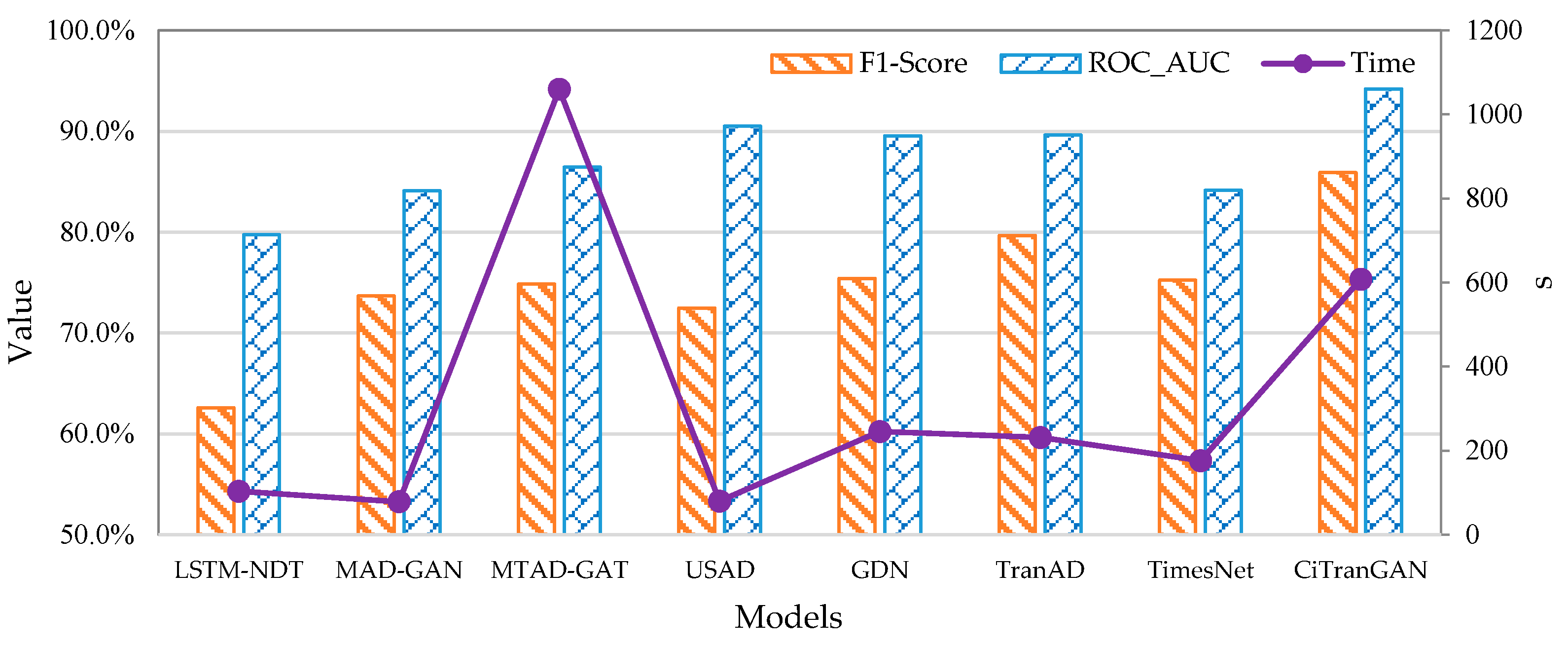
4.4.1. Comparison Experiments with Baseline Models

To validate the effectiveness of CiTranGAN, comparative experiments were performed with seven baseline models across five public datasets. The experimental results are presented in

Table 2. Experimental results of compared to baseline models (%).

		LSTM-NDT	MAD-GAN	MTAD-GAT	USAD	GDN	TranAD	TimesNet	CiTranGAN
SMAP	P	84.13 ± 0.76	81.32 ± 0.72	79.40 ± 0.31	74.33 ± 0.50	74.51 ± 0.62	81.42 ± 0.52	73.01 ± 0.76	87.78 ± 0.57
	R	73.32 ± 0.94	91.53 ± 0.59	97.21 ± 0.32	95.75 ± 0.32	98.12 ± 0.45	98.17 ± 0.41	70.09 ± 0.65	98.98 ± 0.54
	F1	78.35 ± 0.43	86.12 ± 0.55	87.41 ± 0.34	83.69 ± 0.40	84.70 ± 0.52	89.01 ± 0.46	71.52 ± 0.57	93.04 ± 0.46
	Auc	85.58 ± 0.53	98.49 ± 0.53	97.05 ± 0.36	98.10 ± 0.33	98.59 ± 0.35	98.66 ± 0.36	94.29 ± 0.54	98.86 ± 0.30
SWaT	P	77.23 ± 0.73	95.42 ± 0.84	96.67 ± 0.89	98.74 ± 0.68	96.46 ± 0.94	97.21 ± 0.87	98.34 ± 0.89	97.97 ± 0.68
	R	50.67 ± 0.91	69.13 ± 0.83	69.06 ± 0.95	68.51 ± 0.91	69.14 ± 1.05	69.43 ± 0.83	70.14 ± 0.95	81.32 ± 0.87
	F1	61.19 ± 1.04	80.17 ± 0.91	80.57 ± 0.95	80.89 ± 1.06	80.55 ± 1.04	81.00 ± 0.95	81.88 ± 0.92	88.87 ± 0.89
	Auc	70.92 ± 1.02	84.15 ± 1.11	84.12 ± 1.06	84.06 ± 1.13	84.16 ± 1.02	84.40 ± 1.06	83.74 ± 1.07	94.78 ± 0.94
WADI	P	11.53 ± 0.65	22.21 ± 1.00	28.43 ± 0.58	18.69 ± 0.57	29.45 ± 0.54	35.47 ± 0.91	38.29 ± 1.09	46.64 ± 0.64
	R	78.12 ± 1.01	89.23 ± 0.82	80.31 ± 0.50	82.47 ± 0.59	79.18 ± 0.50	82.43 ± 0.82	80.43 ± 0.74	89.47 ± 0.69
	F1	20.09 ± 0.50	35.57 ± 0.88	41.99 ± 0.52	30.47 ± 0.58	42.93 ± 0.56	49.60 ± 0.86	51.88 ± 0.88	61.32 ± 0.63
	Auc	64.46 ± 0.72	68.26 ± 0.70	77.61 ± 0.63	88.68 ± 0.66	78.07 ± 0.61	78.45 ± 0.69	69.01 ± 0.87	81.45 ± 0.53
SMD	P	79.35 ± 0.90	88.91 ± 0.96	79.10 ± 0.60	81.42 ± 0.60	72.69 ± 0.71	89.56 ± 0.64	82.56 ± 0.65	90.28 ± 0.64
	R	79.41 ± 1.16	73.42 ± 0.61	88.12 ± 0.64	84.73 ± 0.65	91.13 ± 0.65	88.24 ± 0.66	89.33 ± 1.10	95.18 ± 0.68
	F1	79.38 ± 0.51	80.43 ± 0.64	83.37 ± 0.66	83.04 ± 0.68	80.87 ± 0.74	88.9 ± 0.65	85.81 ± 0.71	92.67 ± 0.63
	Auc	85.67 ± 0.93	85.64 ± 0.60	81.53 ± 0.67	87.42 ± 0.64	96.69 ± 0.64	92.59 ± 0.67	79.02 ± 0.79	97.83 ± 0.61
MSL	P	62.84 ± 0.95	85.16 ± 0.97	78.63 ± 1.06	79.12 ± 1.04	87.19 ± 1.04	90.08 ± 1.14	82.51 ± 1.16	92.05 ± 0.96
	R	89.91 ± 0.82	86.87 ± 0.86	83.29 ± 0.87	90.13 ± 0.96	88.91 ± 1.05	89.65 ± 1.02	87.97 ± 1.10	95.20 ± 0.65
	F1	73.98 ± 0.98	86.01 ± 0.89	80.89 ± 1.00	84.27 ± 0.94	88.04 ± 1.12	89.86 ± 1.02	85.15 ± 0.71	93.60 ± 0.63
	Auc	92.09 ± 1.01	83.97 ± 0.86	91.89 ± 0.92	94.00 ± 0.88	90.27 ± 1.14	94.05 ± 1.04	94.61 ± 0.79	98.02 ± 0.78

and Figure 10. Here, P, R, F1 and AUC denote Precision, Recall, F1-score, and ROC_AUC, respectively; bold text highlights the best results, while underlined text indicates the second-best results.

Based on the experimental results, compared to the baseline models, CiTranGAN exhibits superior anomaly detection performance across five datasets. However, on the SWaT dataset, the Precision decreased by 0.77% in comparison to USAD. This reduction can be attributed to the high correlation within the dataset’s 51 variables. While CiTranGAN employs a channel-independent strategy to mitigate inter-variable influence, this method also diminishes the model’s ability to capture the dependencies among variables, thereby resulting in the observed drop in Precision. Nevertheless, CiTranGAN achieves notable improvements in Recall, F1-score, and AUC in the SWaT dataset, with gains of 12.81%, 7.98%, and 13.72%, respectively. These results suggest that the benefits of the channel-independent strategy outweigh its drawbacks.

Figure 10 presents the average AUC and F1 scores of all models across the five datasets. Compared to the baseline models, CiTranGAN improves the AUC by a margin ranging from 3.68% to 14.44%, with an average increase of 7.89%. Similarly, its F1-score improves by 6.23% to 23.30%, averaging an enhancement of 12.48%.

In real-world anomaly detection applications, different scenarios may impose varying requirements on evaluation metrics. The F1-score, which considers both Precision and Recall, provides a comprehensive assessment of a model’s performance. Therefore, we focus our analysis primarily on the F1-score in the following discussion. Compared to LSTM-NDT and MAD-GAN, the F1-score showed improvements of 23.30% and 12.24%, respectively. These results demonstrate that CiTranGAN effectively learns vector representations of variables along the temporal dimension, thereby enhancing its anomaly detection capabilities. In contrast, MTAD-GAT and GDN primarily focus on capturing complex data patterns and relationships through graph structures. Relative to these methods, the F1-score of CiTranGAN improved by 11.05% and 10.48%, respectively. This indicates that CiTranGAN’s channel-independent strategy enhances its ability to more effectively capture anomalous information. Compared to USAD, CiTranGAN’s F1-score improved by 13.43%, which demonstrates its superior capability in integrating both local windows and long-term dependencies, thereby addressing USAD’s limitations in accurately classifying long-term anomalies. When compared to TranAD, the F1-score improved by 6.23%. While TranAD employs a self-attention mechanism to capture dependencies between time points, it still fails to adequately account for local variations in the time series data. This highlights the advantage of CiTranGAN’s multi-scale convolutional self-attention mechanism, which enhances its anomaly detection capabilities. Additionally, compared to TimesNet, the F1-score rose by 10.65%, indicating that CiTranGAN is better at uncovering reliable temporal dependencies, thus improving anomaly detection performance.

In summary, for the anomaly detection of MvTS data, CiTranGAN effectively addresses the challenges of high-dimensional data, and achieves the integration of local trends and long-term dependencies. This makes it more focused on capturing general features and trends within the data. As a result, its online training time is relatively high. However, compared to MTAD-GAT, this time is reduced by half. Once trained, CiTranGAN achieves better F1-scores and AUC values than other baseline models, demonstrating outstanding performance in anomaly detection.

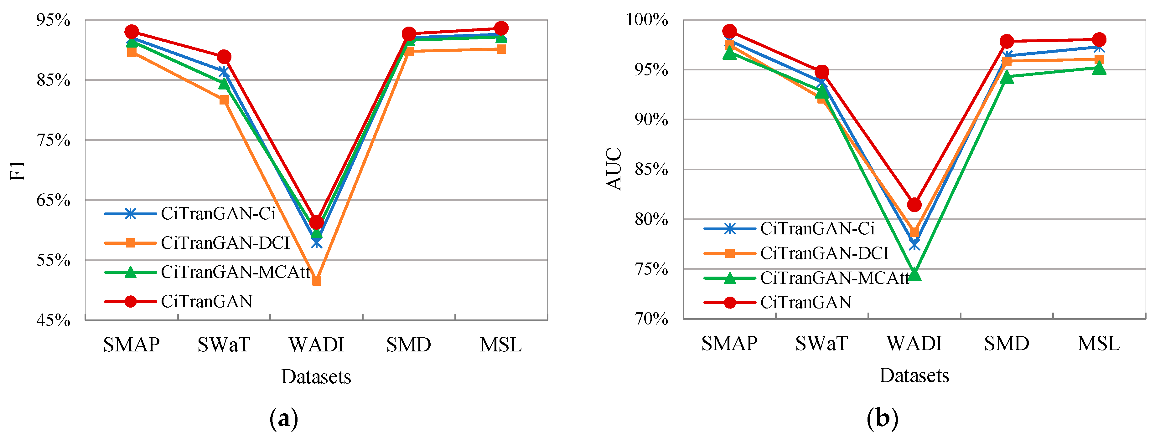
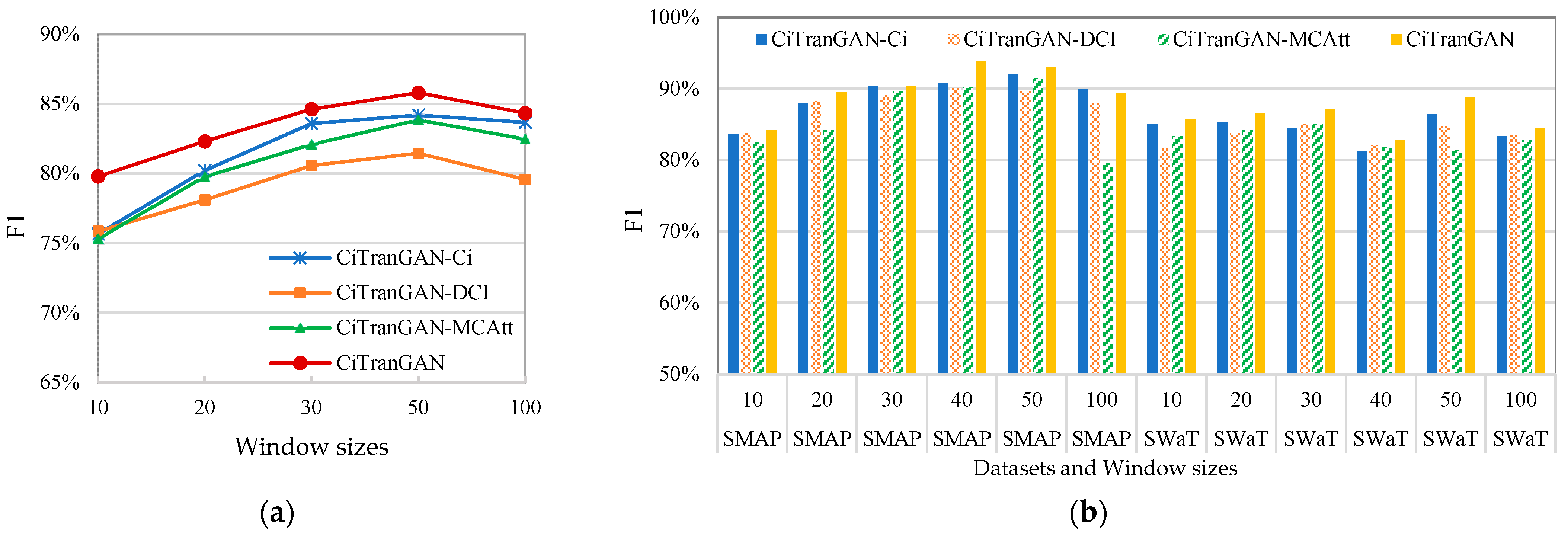
4.4.2. Ablation Experiments

To validate the effectiveness of the three key modules {Ci, DCI, MCAtt} in the CiTranGAN model, ablation experiments were conducted. Specifically, Ci denotes the channel-independence module, DCI denotes the downsampling–convolution–interaction learning module, and MCAtt denotes the multi-scale convolutional self-attention mechanism. In the experiments, CiTranGAN-X indicates the CiTranGAN model without the corresponding module. The experimental results of CiTranGAN and its variants are presented in

Table 3. Ablation experimental results for the CiTranGAN model (%).

		CiTranGAN-Ci	CiTranGAN-DCI	CiTranGAN-MCAtt	CiTranGAN
SMAP	P	86.56 ± 0.54	82.54 ± 0.58	86.45 ± 0.64	87.78 ± 0.57
	R	98.21 ± 0.50	98.11 ± 0.60	97.01 ± 0.57	98.98 ± 0.54
	F1	92.02 ± 0.52	89.65 ± 0.61	91.43 ± 0.63	93.04 ± 0.46
	AUC	97.47 ± 0.49	97.91 ± 0.54	96.72 ± 0.56	98.86 ± 0.30
SWaT	P	95.11 ± 0.70	97.69 ± 0.79	96.07 ± 0.74	97.97 ± 0.68
	R	79.24 ± 0.74	70.21 ± 0.94	75.32 ± 0.79	81.32 ± 0.87
	F1	86.45 ± 0.67	81.70 ± 0.85	84.44 ± 0.95	88.87 ± 0.89
	AUC	92.09 ± 0.85	93.75 ± 0.73	92.84 ± 0.76	94.78 ± 0.94
WADI	P	43.35 ± 0.86	37.69 ± 0.59	44.63 ± 0.67	46.64 ± 0.64
	R	87.23 ± 0.67	81.21 ± 0.54	90.12 ± 0.73	89.47 ± 0.69
	F1	57.92 ± 0.71	51.59 ± 0.68	59.70 ± 0.61	61.32 ± 0.63
	AUC	78.71 ± 0.60	77.45 ± 0.46	74.53 ± 0.59	81.45 ± 0.53
SMD	P	89.41 ± 0.55	89.09 ± 0.71	89.17 ± 0.56	90.28 ± 0.64
	R	94.77 ± 0.68	90.44 ± 0.58	94.14 ± 0.45	95.18 ± 0.68
	F1	92.01 ± 0.40	89.76 ± 0.64	91.59 ± 0.65	92.67 ± 0.63
	AUC	95.86 ± 0.87	96.38 ± 0.70	94.29 ± 0.64	97.83 ± 0.61
MSL	P	90.22 ± 0.90	88.27 ± 0.97	90.17 ± 1.03	92.05 ± 0.96
	R	95.11 ± 0.64	92.11 ± 0.72	94.23 ± 0.75	95.20 ± 0.65
	F1	92.60 ± 0.76	90.15 ± 0.67	92.16 ± 0.78	93.60 ± 0.63
	AUC	96.03 ± 0.94	97.29 ± 0.83	95.22 ± 0.73	98.02 ± 0.78

and Figure 11.

In the five datasets, when the channel-independent module was removed, the F1-score and AUC decreased by an average of 1.70% and 1.63%, respectively. These results indicate that the channel independence strategy plays a crucial role in addressing distribution drift in time series data and mitigating detection challenges caused by increasing data dimensionality. When the DCI was removed, the F1-score and AUC decreased by an average of 2.16% and 4.33%, respectively, indicating that this architecture plays a critical role in enabling cross-temporal-scale feature interaction and learning, which is essential for acquiring more accurate feature representations in the model. Similarly, replacing the MCAtt with the standard multi-head attention mechanism, the F1-score and AUC decreased by an average of 2.04% and 3.47%, respectively, highlighting the significant impact of similar subsequence relationships on time series anomaly detection tasks.

In summary, the ablation experiments conclusively validate the necessity of all three modules, offering robust theoretical and empirical evidence for both the architectural design and the performance enhancements of CiTranGAN.

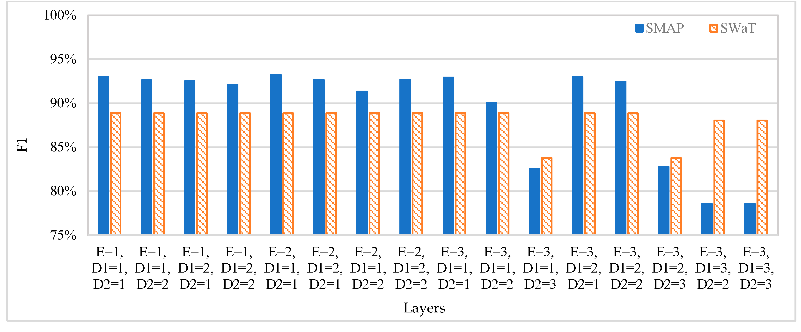
4.4.3. Sensitivity Experiments

Under varying window sizes, experimental verification and comparative analysis of the CiTranGAN model and its variants were carried out. The F1-score results are shown in Figure 12. The findings demonstrate that the window size significantly influences the anomaly detection performance. With a smaller window size (W = 10), CiTranGAN fails to capture essential long-term dependencies, resulting in suboptimal performance. As the window size increases from 10 to 50, the F1-score gradually improves, indicating that larger windows enable the model to better utilize long-term information. However, when the window size reaches 100, excessive redundancy in the early data becomes apparent, which negatively impacts current predictions and diminishes model performance. We can see from Figure 12b that there remain notable variations in the sensitivity of different datasets to window size. Specifically, CiTranGAN demonstrates superior performance when the SMAP window size is set to 40. Conversely, under a window size of 40 for SWaT, the overall performance is relatively poor. In summary, these findings suggest that a window size of 50 is most appropriate for CiTranGAN models and their variants.

In order to deeply explore the influence of the number of encoder and decoder layers on the performance of the CiTranGAN model, a set of experiments were designed on SMAP and SWaT datasets while keeping other hyperparameters unchanged, as shown in Figure 13. The experiments show that, across various datasets, there are significant differences in the influence of the number of encoder and decoder layers configured on the model performance. Specifically, in SMAP, as the number of encoder layers increases, the effect of anomaly detection improves to a certain extent. However, as the number of decoder layers increases, the detection effect decreases. The effect is the best when E = 2, D1 = 1, and D2 = 1. It increased by 0.21% compared with E = 1, D1 = 1, and D2 = 1. In SWaT, when E ≤ 2, the change in the number of layers has no impact on performance. When the number of layers in both the encoder and decoder reaches 3, there is a significant decrease in performance in both datasets. This could be attributed to the fact that excessively deep networks are more susceptible to issues such as gradient vanishing or gradient explosion, thereby increasing the complexity of model training. In this paper, by comprehensively considering machine performance and computational complexity, both the encoder and decoder are configured with a single layer. In practical applications, the number of layers for both the encoder and decoder can be further adjusted in accordance with the specific dataset and task requirements to achieve optimal performance.

4.5. Limitations and Future Work

The CiTranGAN model presented in this paper shows superior performance in the anomaly detection of MvTS data, but there are still some limitations. Below are the detailed limitations of this study:

• The CI strategy ignores the inter-variable correlation. Although the strategy effectively alleviates the distribution drift problem in time series data, it treats each variable as an independent single variable and ignores the potential correlation between variables. In some scenarios, inter-variable correlations play a critical role in anomaly detection, and disregarding these relationships may result in reduced model accuracy on specific datasets, as evidenced by the experimental results on the SWaT dataset.
• Limited generalization capability. The experimental results presented in this paper are primarily derived from five public datasets, which, despite their representativeness, may not fully capture the complexities and variations in data in specific domains or scenarios. Consequently, the model’s performance in practical applications could be influenced by domain-specific data characteristics. Further validation is therefore required to comprehensively assess the model’s generalization capability.
• High computational complexity and resource consumption. While the CiTranGAN model demonstrates excellent performance across multiple datasets, its computational demands are relatively high, particularly when processing large-scale time series data. The multi-scale convolutional self-attention mechanism and the generative adversarial network architecture within the model necessitate substantial computational resources and memory capacity, thereby restricting its applicability in resource-constrained environments. This may introduce time constraints during the actual deployment and updating of the model.
• Parameter sensitivity and challenges in tuning. The CiTranGAN model incorporates several hyperparameters, including the size of the sliding window, the number of encoder layers, and the dimension of the convolution kernel. The choice of these parameters significantly influences model performance; however, identifying the optimal parameter combination remains a complex challenge. Moreover, since different datasets may necessitate distinct parameter configurations, this further complicates the tuning process.
• Lack sufficient explanation. While the model demonstrates high accuracy in anomaly detection, its ability to explain anomalies remains inadequate. In practical applications, users are not only interested in identifying the presence of exceptions but also in understanding their underlying causes and sources. Consequently, enhancing the interpretability of the model is crucial for building user trust and providing robust decision support.

In summary, the CiTranGAN model introduced in this paper has demonstrated significant achievements in the anomaly detection of multivariable time series data. However, it still exhibits certain limitations. Future research could focus on addressing and optimizing these limitations to enhance the model’s generalization capability, reduce computational complexity, and improve parameter stability and anomaly interpretability.

5. Conclusions

Based on Transformer, GAN, and channel-independent strategies, this paper proposes a novel multivariate time series anomaly detection model, CiTranGAN. This model leverages a channel-independent strategy to mitigate the challenges associated with high dimensionality and distribution drift in data. Through the time series feature extraction module, it facilitates the collaborative learning of features at various time scales, thus reducing the effects of temporal redundancy. Additionally, by utilizing a hybrid dilated causal convolution, a multi-scale convolutional self-attention mechanism is designed, which not only captures the local trends but also effectively identifies long-term dependencies. The experimental results on five real-world datasets demonstrate that CiTranGAN outperformed seven baseline models, with the AUC improved by a margin ranging from 3.68% to 14.44%, an average increase of 7.89%. Similarly, the F1-score improved by 6.23% to 23.30%, averaging an enhancement of 12.48%. In the ablation experiments, the channel independence, downsampling–convolution–interaction learning, and multi-scale convolutional self-attention mechanism contributed improvements in AUC of 1.63%, 2.16%, and 3.47; similarity, improvements in F1-score of 1.70%, 4.33%, and 2.04%, respectively, were observed. These findings underscore the robust anomaly detection capabilities of CiTranGAN. Future research will focus on developing a sparse self-attention mechanism to further enhance anomaly detection accuracy under lower spatiotemporal complexity.

References

- Pau, F.C.; Jose, M.B.; Jorge, G.V. A Review of Graph-Powered Data Quality Applications for IoT Monitoring Sensor Networks. J. Netw. Comput. Appl. 2025, 1, 104116. [Google Scholar] [CrossRef]
- Thudumu, S.; Branch, P.; Jin, J.; Singh, J.J. A comprehensive survey of anomaly detection techniques for high dimensional big data. J. Big Data 2020, 7, 42. [Google Scholar] [CrossRef]
- Chandola, V.; Mithal, V.; Kumar, V. Comparative Evaluation of Anomaly Detection Techniques for Sequence Data. In Proceedings of the 8th IEEE International Conference on Data Mining, Pisa, Italy, 15–19 December 2008; pp. 743–748. [Google Scholar]
- Leon-lopez, K.M.; Mouret, F.; Arguello, H.; Tourneret, J.Y. Anomaly detection and classification in multispectral time series based on hidden Markov models. IEEE Trans. Geosci. Remote Sens. 2021, 60, 5402311. [Google Scholar] [CrossRef]
- Erhan, L.; Ndubuaku, M.; Di Mauro, M.; Song, W.; Chen, M.; Fortino, G.; Bagdasar, O.; Liotta, A. Smart anomaly detection in sensor systems: A multi-perspective review. Inf. Fusion 2021, 67, 64–79. [Google Scholar] [CrossRef]
- Lu, Y.; Wu, R.; Mueen, A.; Zuluaga, M.A.; Keogh, E.J. Matrix Profile XXIV: Scaling Time Series Anomaly Detection to Tril-lions of Datapoints and Ultra-Fast Arriving Data Streams. In Proceedings of the 28th ACM SIGKDD Conference on Knowledge Discovery and Data Mining, New York, NY, USA, 14–18 August 2022; pp. 1173–1182. [Google Scholar]
- Li, Y.; Chen, Z.; Zha, D.; Du, M.; Zhang, D.; Chen, H.; Hu, X. Towards Learning Disentangled Representations for Time Series. In Proceedings of the 28th ACM SIGKDD Conference on Knowledge Discovery and Data Mining, New York, NY, USA, 14–18 August 2022; pp. 3270–3278. [Google Scholar]
- Liu, Y.; Zhou, Y.J.; Yang, K.; Wang, X. Unsupervised deep learning for IoT time series. IEEE Internet Things J. 2023, 10, 14285–14306. [Google Scholar] [CrossRef]
- Hundman, K.; Constantinou, V.; Laporte, C.; Colwell, I.; Soderstrom, T. Detecting Spacecraft Anomalies Using LSTMs and Nonparametric Dynamic Thresholding. In Proceedings of the 24th ACM SIGKDD International Conference on Knowledge Discovery & Data Mining, London, UK, 19–23 August 2018; pp. 387–395. [Google Scholar]
- Audibert, J.; Michiardi, P.; Guyard, F.; Marti, S.; Zuluaga, M.A. USAD: Unsupervised Anomaly Detection on Multivariate Time Series. In Proceedings of the 26th ACM SIGKDD International Conference on Knowledge Discovery & Data Mining, New York, NY, USA, 23–27 August 2020; pp. 3395–3404. [Google Scholar]
- Tuli, S.; Casale, G.; Jennings, N.R. TranAD: Deep Transformer networks for anomaly detection in multivariate time series data. In Proceedings of the 48th International Conference on Very Large Data Bases, Sydney, Australia, 5–9 September 2022; pp. 1201–1214. [Google Scholar] [CrossRef]
- Rabanser, S.; Januschowski, T.; Flunkert, V.; Salinas, D.; Gasthaus, J. The effectiveness of discretization in forecasting: An empirical study on neural time series models. arXiv 2020, arXiv:2005.10111. [Google Scholar]
- Zeng, A.; Chen, M.; Zhang, L.; Xu, Q. Are Transformers Effective for Time Series Forecasting? arXiv 2022, arXiv:2205.13504. [Google Scholar] [CrossRef]
- Breunig, M.M.; Kriegel, H.P.; Ng, R.T.; Sander, J. LOF: Identifying Density-Based Local Outliers. In Proceedings of the 2000 ACM SIGMOD International Conference on Management of Data, Dallas, TX, USA, 15–18 May 2000; pp. 93–104. [Google Scholar]
- Kim, J.S.; Scott, C.D. Robust kernel density estimation. J. Mach. Learn. Res. 2012, 13, 2529–2565. [Google Scholar]
- Shyu, M.L.; Chen, S.C.; Sarinnapakorn, K.; Chang, L. A Novel Anomaly Detection Scheme Based on Principal Component Classifier. In Proceedings of the IEEE Foundations and New Directions of Data Mining Workshop, Piscataway, NJ, USA, 19–22 November 2003; pp. 172–179. [Google Scholar]
- Candès, E.J.; Li, X.D.; Ma, Y.; Wright, J. Robust principal component analysis? J. ACM 2009, 58, 1–37. [Google Scholar] [CrossRef]
- Hautamaki, V.; Karkkainen, I.; Franti, P. Outlier Detection Using K-Nearest Neighbour Graph. In Proceedings of the 17th International Conference on Pattern Recognition, Cambridge, UK, 23–26 August 2004; IEEE: New York, NY, USA, 2004; pp. 430–433. [Google Scholar]
- Zhang, Y.; Hammn, A.S.; Meratnia, N.; Stein, A.; Van, V.M.; Havinga, J.M. Statistics-based outlier detection for wireless sensor networks. Int. J. Geogr. Inf. Sci. 2012, 26, 1373–1392. [Google Scholar] [CrossRef]
- Fei, T.L.; Kai, M.T.; Zhou, Z.H. Isolation forest. In Proceedings of the 8th IEEE International Conference on Data Mining, Pisa, Italy, 15–19 December 2008; IEEE: New York, NY, USA, 2008; pp. 413–422. [Google Scholar]
- Barrera-Llanga, K.; Burriel-Valencia, J.; Sapena-Bano, A.; Martinez-Roman, J. Fault detection in induction machines using learning models and fourier spectrum image analysis. Sensors 2025, 25, 471. [Google Scholar] [CrossRef] [PubMed]
- Malhotra, P.; Vig, L.; Shroff, G.; Agarwal, P. Long Short Term Memory Networks for Anomaly Detection in Time Series. In Proceedings of the 23th European Symposium on Artificial Neural Networks, Bruges, Belgium, 22–24 April 2015; pp. 89–94. [Google Scholar]
- Nanduri, A.; Sherry, L. Anomaly Detection in Aircraft Data Using Recurrent Neural Networks (RNN). In Proceedings of the 16th Integrated Communications Navigation and Surveillance, Herndon, VA, USA, 19–24 April 2016; pp. 1–8. [Google Scholar]
- Guo, Y.; Liao, W.; Wang, Q.; Yu, L.X.; Ji, T.X.; Li, P.M. Multidimensional Time Series Anomaly Detection: A Gru-Based Gaussian Mixture Variational Autoencoder Approach. In Proceedings of the Asian Conference on Machine Learning, Tokyo, Japan, 8–10 November 2018; pp. 97–112. [Google Scholar]
- Xia, T.B.; Song, Y.; Zheng, Y.; Pan, E.; Xi, L.F. An ensemble framework based on convolutional bi-directional LSTM with multiple time windows for remaining useful life estimation. Comput. Ind. 2020, 115, 103182–103196. [Google Scholar] [CrossRef]
- Li, T.; Comer, M.L.; Delp, E.J.; Desai, S.R.; Chan, M.W. Anomaly Scoring for Prediction-Based Anomaly Detection in Time Series. In Proceedings of the IEEE Aerospace Conference, Bozeman, MT, USA, 7–14 March 2020; pp. 1–7. [Google Scholar]
- Chen, Z.; Chai, K.Y.; Bu, S.L.; Lau, C.T. Autoencoder-Based Network Anomaly Detection. In Proceedings of the Wireless Tele-communications Symposium Conference, Los Angeles, CA, USA, 4–6 April 2018; pp. 1–5. [Google Scholar]
- Xu, H.; Feng, Y.; Chen, J.; Wang, Z.; Qiao, H.; Chen, W.; Zhao, N.; Li, Z.; Bu, J.; Li, Z. Unsupervised Anomaly Detection via Variational Auto-Encoder for Seasonal Kpis in Web Applications. In Proceedings of the 2018 World Wide Web Conference, Paris, France, 23–27 April 2018; pp. 187–196. [Google Scholar]
- Park, D.; Hoshi, Y.; Kemp, C.C. A multimodal anomaly detector for robot-assisted feeding using an lstm-based variational autoencoder. IEEE Robot. Autom. Lett. 2018, 3, 1544–1551. [Google Scholar] [CrossRef]
- Li, D.; Chen, D.; Jin, B.; Goh, J.; Ng, S.K. MAD-GAN: Multivariate Anomaly Detection for Time Series Data with Generative Adversarial Networks. In Proceedings of the International Conference on Artificial Neural Networks, Munich, Germany, 16–19 September 2019; pp. 703–716. [Google Scholar]
- Vaswani, A.; Shazeer, N.; Parmar, N.; Uszkoreit, J.; Jones, L.; Gomez, A.N.; Kaiser, L.; Polosukhin, I. Attention is all you need. In Proceedings of the 31st Conference on Neural Information Processing Systems, Long Beach, CA, USA, 4–9 December 2017; pp. 30–40. [Google Scholar]
- Xu, J.H.; Wu, H.X.; Wang, J.M.; Long, M.S. Anomaly Transformer: Time Series Anomaly Detection with Association Dis-crepancy. In Proceedings of the International Conference on Learning Representations, Lyon, France, 25–29 April 2022; pp. 1021–1038. [Google Scholar]
- Du, B.; Sun, X.; Ye, J. GAN-based anomaly detection for multivariate time series using polluted training set. IEEE Transac-Tions Knowl. Data Eng. 2021, 35, 12208–12219. [Google Scholar] [CrossRef]
- Wu, H.; Yang, R.; Qing, H. TSFN: An Effective Time Series Anomaly Detection Approach via Transformer-based Self-feedback Network. In Proceedings of the 26th International Conference on Computer Supported Cooperative Work in Design (CSCWD), Kunming, China, 24–26 May 2023; pp. 1396–1401. [Google Scholar]
- Wang, Z.; Wang, Y.; Gao, C.; Wang, F.; Lin, T.; Chen, Y. An adaptive sliding window for anomaly detection of time series in wireless sensor networks. Wirel. Netw. 2022, 28, 393–411. [Google Scholar] [CrossRef]
- Shaukat, K.; Alam, T.M.; Luo, S.; Shabbir, S.; Javed, U. A Review of Time-Series Anomaly Detection Techniques: A Step to Future Perspectives. In Proceedings of the 2021 Future of Information and Communication Conference, Beijing, China, 22–24 October 2021; pp. 865–877. [Google Scholar]
- Arnold, B.C. Pareto and generalized Pareto distributions. In Modeling Income Distributions and Lorenz Curves; Springer: New York, NY, USA, 2008; pp. 119–145. [Google Scholar]
- Lazar, N.A. Statistics of Extremes: Theory and Applications. Technometrics 2005, 47, 376–377. [Google Scholar] [CrossRef]
- Han, L.; Ye, H.J.; Zhan, D.C. The capacity and robustness trade-off: Revisiting the channel independent strategy for multivariate time series forecasting. IEEE Trans. Autom. Control. 2024, 36, 14. [Google Scholar] [CrossRef]
- Luo, J.H.; Wu, J. Neural Network Pruning with Residual-Connections and Limited-Data. In Proceedings of the IEEE/CVF conference on Computer Vision and Pattern Recognition, Seattle, WA, USA, 14–19 June 2020; pp. 1458–1467. [Google Scholar]
- Szegedy, C.; Liu, W.; Jia, Y.; Sermanet, P.; Reed, S.; Anguelov, D.; Erhan, D.; Vanhoucke, V.; Rabinovich, A. Going Deeper with Convolutions. In Proceedings of the IEEE Conference on Computer Vision and Pattern Recognition, Boston, MA, USA, 7–12 June 2015; pp. 1–9. [Google Scholar]
- Zhao, H.; Wang, Y.; Duan, J.; Huang, C.; Cao, D.F.; Tong, Y.H.; Xu, B.X.; Bai, J.; Tong, J.; Zhang, Q. Multivariate Time-Series Anomaly Detection Via Graph Attention Network. In Proceedings of the 2020 IEEE International Conference on Data Mining, Istanbul, Turkey, 30–31 July 2020; pp. 841–850. [Google Scholar]
- Deng, A.; Hooi, B. Graph Neural Network-Based Anomaly Detection in Multivariate Time Series. In Proceedings of the AAAI Conference on Artificial Intelligence, Vancouver, BC, Canada, 9–12 February 2021; pp. 4027–4035. [Google Scholar]
- Wu, H.X.; Hu, T.G.; Liu, Y.; Zhou, H.; Wang, J.M.; Long, M.S. Timesnet: Temporal 2d-Variation Modeling for General Time Series Analysis. In Proceedings of the 11th International Conference on Learning Representations, Kigali, Rwanda, 1–5 May 2023; pp. 135–158. [Google Scholar]