A Multi-Receiver Pulse Deinterleaving Method Based on SSC-DBSCAN and TDOA Mapping

Abstract

Deinterleaving pulses of various pulse repetition interval (PRI) modulation modes constitute a vital and challenging task for an electronic measures system (ESM). A deinterleaving method based on multi-receiver time-difference-of-arrival (TDOA) is proposed in this paper. Firstly, this paper theoretically analyzes the distribution feature of TDOA, providing the basis of deinterleaving. Then, a SSC (Sorting Skipping Clustering)-DBSCAN algorithm is proposed to achieve TDOA clustering by pre-sorting and traversing key points, which reduces the computational complexity. The TDOA mapping algorithm is further proposed to separate pulses and eliminate Cross-Pulse TDOAs simultaneously based on a one-time clustering result, which can significantly decrease the false alarm rate while avoiding clustering TDOA repeatedly. Simulation results show that the proposed method is capable of deinterleaving pulses of various PRI modulation modes and the performance remains excellent under multiple parameter settings. The running time and the false alarm rate have been reduced by at least 66% and 17%, respectively, compared with the existing methods.

1. Introduction

Radar pulse deinterleaving refers to the process of separating the pulse sequences corresponding to each radar from an interleaved sequence, which plays an important role in electronic measure (ESM) systems. The correct pulse deinterleaving result is a prerequisite for the precise emitter identification and accurate threat assessment of radars [1]. The pulses intercepted by the ESM system are described as pulse description words (PDWs), which contains five basic parameters, radio frequency (RF), pulse width (PW), pulse amplitude (PA), direction of arrival (DOA), and time of arrival (TOA) [2]. With the rapid development of radar technology, various kinds of radars with complex pulse repetition interval (PRI) modulation modes are used in modern warfare, which poses significant challenges to pulse deinterleaving [3].

Based on PDWs, plenty of studies have been conducted in pulse deinterleaving for single-receiver ESM systems over the past years, which can be mainly divided into TOA-based methods and multi-parameter-based methods. Besides, time-difference-of-arrival (TDOA) of multi-receiver ESM systems has been introduced to pulse deinterleaving recently. The pulse repetitive interval (PRI) refers to the time interval between two adjacent pulses in a pulsed signal. In TOA-based methods, PRI is estimated through the difference of TOA and exploited to distinguish the pulses belonging to different radars. TOA-based methods mainly include histogram-based methods [4,5,6,7,8], PRI-transformation-based methods [9,10,11,12] and clustering-based methods [13,14,15]. The TOA-based methods above show good performance for some pulse modulation modes such as PRI-fixed pulses. However, they are not always effective for interleaved pulses of various PRI modulation modes, since the TOA differences are sensitive to the PRI modulation modes. Multi-parameter-based methods deinterleave pulses by combining TOA with other PDWs [16]. Neural networks have been introduced by using small time units to digitize time information such as TOA and PW [17]. The instance segmentation network is applied for end-to-end deinterleaving by encoding a PDW to a 2D RF-TOA image [18,19,20], which decreases the dependence on the presetting parameter. However, these methods can deinterleave pulse trains just for a short period of time with long running time relatively. Besides, they are not suitable for adversarial environments due to the dependence on training samples.

For an ESM system with multiple receivers, it is worth noting that the time difference of arrival (TDOA) of a certain pulse at different receivers is only determined by the position of the emitter [21]. As the emitter changes relatively slowly due to the limited speed, TDOA is more robust compared with PDWs, independently of the PRI modulation modes [22]. Using TDOA for deinterleaving can separate pulses with various PRI modulation modes, but it faces the problems of high false alarm rate and computational complexity caused by Cross-Source TDOA. TDOA-based methods can be divided into the following two categories: histogram-based and clustering-based. In histogram-based methods, an extended histogram is proposed to eliminate Cross-Source TDOA based on the distribution of the TDOA values [23], and PDW constraints are further introduced to reduce the initial noise of the histogram [24,25,26]. The false alarm rates of these methods are reduced, but the computational complexity is high since the extended histogram needs to be calculated repeatedly. Clustering-based methods [27,28] reduce the computational complexity but have a high false alarm rate due to the Cross-Pulse TDOA not being effectively eliminated. In addition, the performance of most of the aforementioned TDOA methods greatly depends on the presetting parameters.

The distribution feature of TDOA is theoretically analyzed in this paper, providing the basis of pulse deinterleaving. In order to deinterleave pulses of various modulation modes, this paper proposes a real-time multi-receiver pulse deinterleaving method based on Density-Based Spatial Clustering of Applications with Noise (DBSCAN) and TDOA mapping, which corrects the defects of the above TDOA methods. This method deinterleave pulses through the following three steps: TDOA extracting, TDOA clustering, and TDOA mapping. The contributions of this paper are summarized as follows:

1.

An efficient clustering algorithm Sorting Skipping Clustering (SSC)-DBSCAN is proposed. SSC-DBSCAN clusters TDOA by pre-sorting and traversing key points, which has a low time complexity of $O(nlogn)$.

2.

A TDOA mapping algorithm is proposed, which separates pulses and eliminate Cross-Source TDOAs simultaneously based on a one-time clustering result. As a result, the false alarm rate has significantly decreased while avoiding clustering TDOA repeatedly.

3.

Extensive simulation results show that the proposed method can deinterleave pulses of various PRI modulation modes. The running time and the false alarm rate have been reduced by at least 66% and 17%, respectively, compared with other TDOA methods.

The rest of this paper is organized as follows. Section 2 introduces a model for a multi-receiver ESM system and the distribution features of the TDOA value of the pulses at different receivers. Section 3 shares the details of the proposed method. Section 4 provides simulations and analysis. Finally, Section 5 concludes this paper.

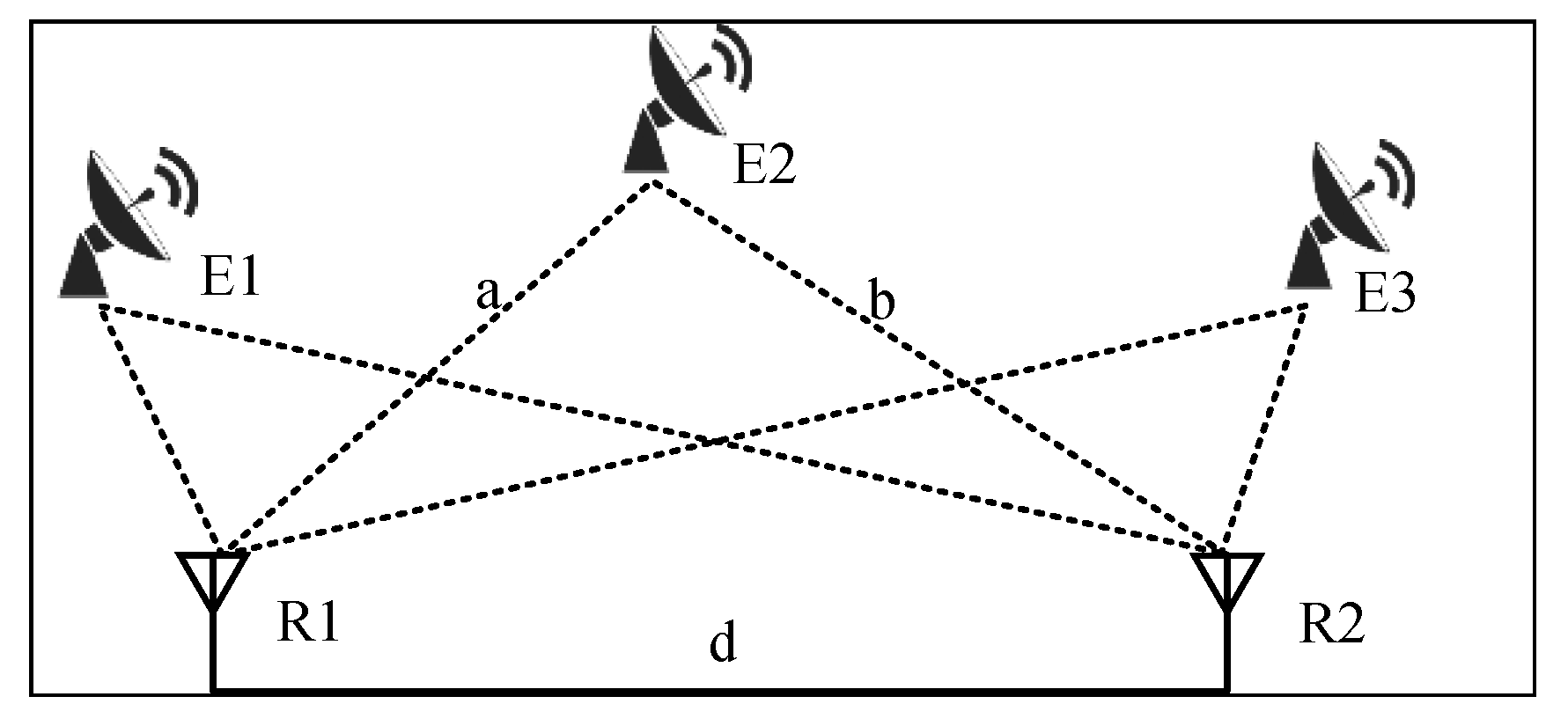
2. System Model and TDOA Distribution Analysis

In the various types of TDOAs generated by a multi-receiver ESM system, the TDOA of the same pulse received by two receivers (defined as Same-Pulse TDOA in this paper) has a one-to-one mapping relationship. This is the basis for radar pulse deinterleaving using TDOA. However, other types of TDOAs exist, which affect the false alarm rate and accuracy of the deinterleaving results. Therefore, the primary problem to be solved is how to distinguish Same-Pulse TDOA and eliminate the influence of other types of TDOAs.

To address the above issues, this section presents the generation model of the TDOA sequence in a multi-receiver ESM system and classifies different TDOA types firstly. Then, the quantitative distribution characteristic of different TDOAs is derived, which is the main basis for distinguishing Same-Pulse TDOA from other types of TDOAs in the following method.

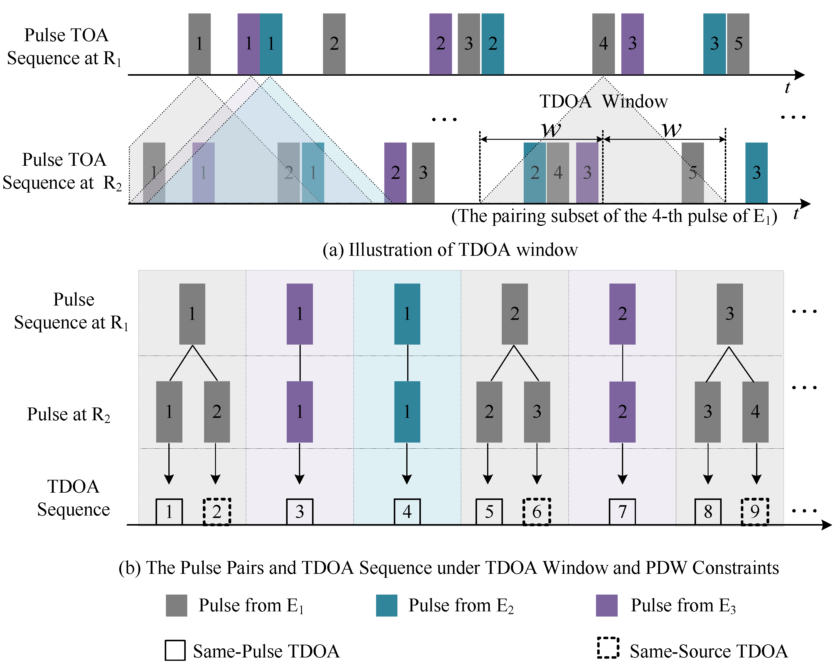
2.1. TDOA Sequence and TDOA Types

The ESM system with two receivers is shown in Figure 1, where $R_1$ and $R_2$ are the primary receiver and the secondary receiver, respectively. There are three radars, $E_1$, $E_2$, and $E_3$, within the detectable range. $R_1$ and $R_2$ independently intercept the pulse signals emitted by these radars, and $R_2$ sends the intercepted pulses to $R_1$ for further processing. The observation time of the ESM is T. Assume that the positions of $R_1$, $R_2$, $E_1$, $E_2$, and $E_3$ are relatively unchanged and the quantity of pulses received by both $R_1$ and $R_2$ is N within T. There are $N^2$ possible pairwise combinations between the pulses received by $R_1$ and those received by $R_2$, which can correspondingly generate $N^2$ TDOAs. These TDOAs can be divided into two major types or three sub-types [23].

• Same-Pulse TDOA refers to the TOA difference of the same pulse received by $R_1$ and $R_2$.
• Cross-Pulse TDOA refers to the TOA difference of two different pulses received by $R_1$ and $R_2$. Cross-Pulse TDOA can be divided into the following two types: Same-Source TDOA and Cross-Source TDOA, which are denoted as follows.

  -

  Same-Source TDOA refers to the TOA difference of two different pulses received by $R_1$ and $R_2$, where the two pulses are from the same radar.

  -

  Cross-Source TDOA refers to the TOA difference of two different pulses received by $R_1$ and $R_2$, where the two pulses are from two different radars.

Among the generated $N^2$ TDOAs, only Same-Pulse TDOAs are useful, while the remaining Cross-Pulse TDOAs will affect the result of pulse deinterleaving. Therefore, it is necessary to reduce the generation of Cross-Pulse TDOAs by adding constraints.

Denote ${\tau }_{SP}$ as a value of Same-Pulse TDOA. As shown in Figure 1, taking the Same-Pulse TDOA of $E_2$ as an example, ${\tau }_{SP}$ satisfies

$$|{\tau }_{SP}|={\displaystyle \frac{|a-b|}{c}}<{\displaystyle \frac{d}{c}}=w$$

(1)

where a is the distance between $E_2$ and $R_1$, b is the distance between $E_2$ and $R_2$, c is the speed of light, d is the distance between $R_1$ and $R_2$, and w is the time taken for light to travel from $R_1$ to $R_2$. It shows that Same-Pulse TDOA ${\tau }_{SP}$ is only related to the position of the radar and satisfies ${\tau }_{SP}\in \left(-w,w\right)$, which is referred to as the TDOA window constraint. Due to the almost constant position of the radar during the observation time of the ESM system, the Same-Pulse TDOA values for the same radar are theoretically equal.

The parameters RF and PW of the same pulse measured by R1 and R2 are nearly identical, while those of the pulses from different radars differ. Assuming that the i-th pulse in the $R_1$ sequence and the j-th pulse in the $R_2$ sequence are the same pulse, the PDWs of the same pulse measured by $R_1$ and $R_2$ satisfy

$$\left\{\begin{array}{c}\left|PD{W}_1\left(i\right).\mathrm{RF}-\mathrm{PD}{\mathrm{W}}_2\left(\mathrm{j}\right).\mathrm{RF}\right|<2{\sigma }_r\hfill \\ \left|PD{W}_1\left(i\right).\mathrm{PW}-\mathrm{PD}{\mathrm{W}}_2\left(\mathrm{j}\right).\mathrm{PW}\right|<2{\sigma }_p\hfill \end{array}\right.$$

(2)

where $PD{W}_1\left(i\right)$ represents the PDW of the i-th pulse in the $R_1$ sequence, $PD{W}_2\left(j\right)$ represents the PDW of the j-th pulse in the $R_2$ sequence, and ${\sigma }_r$ and ${\sigma }_p$ are the maximum measurement errors of the RF and PW for the ESM system, respectively. (2) is referred as the PDW constraint.

Figure 2a depicts the pulse TOA sequences at $R_1$ and $R_2$, where rectangles represent pulses as follows: the color of each rectangle indicates the radar source, and the number of each rectangle denotes the transmission order of pulses from the same radar. Figure 2b illustrates the pulse pair between $R_1$ and $R_2$ under the TDOA window and PDW constraints. As shown in Figure 2a, the pairing scope for each pulse in the $R_1$ sequence can be narrowed from the entire $R_2$ sequence to a corresponding constrained subset through the TDOA window constraint. As Figure 2b illustrates, pulses in these $R_2$ subsets whose radar emitters differ from the corresponding pulses at $R_1$ will be eliminated under the PDW constraint. Since Cross-Source TDOA is the TOA difference of two pulses from different radars, Cross-Source TDOA will not be generated under the TDOA window and PDW constraints. There are Same-Pulse TDOAs and Same-Source TDOAs in the generated TDOA sequence. The following will analyze the quantity distribution features of the two types of TDOAs.

2.2. Quantity Distribution of TDOAs

Assume that the receiver $R_1$ and $R_2$ of the ESM have intercepted the same pulses within T, which are from M radars. The TOA sequence of pulses intercepted by $R_n$ from radar $E_m$ can be represented as follows:

$$x_{n,m}\left(t\right)={\displaystyle \sum _{i=1}^{N_m}}\delta (t-t_{n,m}^i),n=1,2;m=1,2,\cdots ,M$$

(3)

where $\delta \left(t\right)$ is the unit impulse function and $\delta (t-t_{n,m}^i)$ represents the $i-\mathrm{th}$ pulse from $E_m$ intercepted from $R_n$. The quantity of TDOA with the value of ${\tau }_0$ for radar $E_m$ is as follows:

$$h\left({\tau }_0\right)={\int }_{{\tau }_0^{-}}^{{\tau }_0^{+}}\sum _{i=1}^{N_m}\sum _{j=1}^{N_m}\delta [\tau -(t_{1,m}^j-t_{2,m}^i\left)\right]d\tau ,\tau \in [-w,w]$$

(4)

2.2.1. Quantity of Same-Pulse TDOAs for Radar $E_m$

Denote the value of Same-Pulse TDOA for radar $E_m$ as ${\tau }_{SP}$, then, the quantity of Same-Pulse TDOA for radar $E_m$ within T can be represented as

$$h\left({\tau }_{SP}\right)={\int }_{{{\tau }_{SP}}^{-}}^{{{\tau }_{SP}}^{+}}\sum _{i=1}^{N_m}\delta (\tau -{\tau }_{SP})d\tau =N_m$$

(5)

where $N_m$ is the quantity of pulses from $E_m$ within T.

2.2.2. Quantity of Same-Source TDOAs with Equal Value for Radar $E_m$

If the PRI of the pulses from $E_m$ satisfies (6), there will be Same-Source TDOAs related to $E_m$.

$$PRI<w - |{\tau }_{SP}|$$

(6)

where ${\tau }_{SP}$ represents the Same-Pulse TDOA value of $E_m$. If the PRI of radar $E_m$ is fixed, then, the quantity of Same-Source TDOA with the value of ${\tau }_{S{S}_p}$ within T is

$$\begin{array}{cc}\hfill & {\tau }_{S{S}_p}=p·PRI+{\tau }_{SP},p=1,2,\cdots ;\left|{\tau }_{S{S}_p}\right|<w\hfill \\ \hfill & h\left({\tau }_{S{S}_p}\right)={\int }_{{\tau }_p^{-}}^{{\tau }_p^{+}}\sum _{k=1}^{N_m-\left|p\right|}\delta \left[\tau -\left(t_{1,m}^k-t_{2,m}^{k+\left|p\right|}\right)\right]d\tau =N_m-\left|p\right|\hfill \end{array}$$

(7)

where p is the quantity of PRIs for $E_m$ satisfying $\left|{\tau }_{S{S}_p}\right|<w$.

In addition to fixed PRI, the PRI modulation methods of radar also include stagger PRI, jitter PRI, sliding PRI and group PRI, etc. If the PRI of $E_m$ is not fixed, the quantity of Same-Source TDOAs with an equal value will decrease with a decrease in equal PRIs.

Based on the above analysis, the following conclusions can be established. The quantity of Same-Pulse TDOA with equal value is more than those of Same-Source TDOA with equal value or Cross-Source TDOAs with equal value for the same radar. Consequently, when clustering the TDOA values, the cluster with the highest quantity is the Same-Pulse TDOA cluster, which maps to a pulse sequence of a certain radar.

3. Proposed Deinterleaving Method

According to the analysis in Section 2, the deinterleaving process can be designed as follows. Firstly, generate TDOAs based on the joint constraints of the TDOA window and PDWs. Secondly, cluster the TDOA values. Then, deinterleave the pulses based on the cluster with the highest quantity. Finally, remove the related TDOAs of the deinterleaved pulses systematically from the TDOA cluster and repeat the above operations on the remaining data until all the pulses have been deinterleaved.

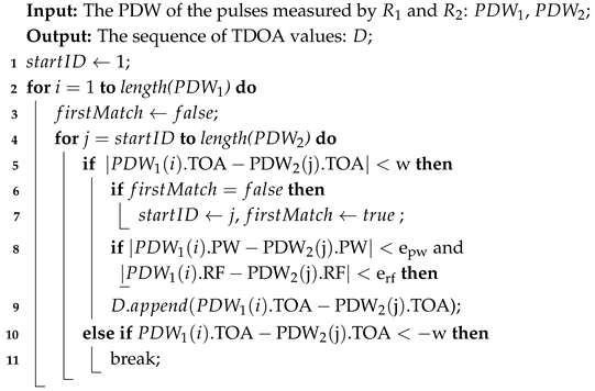
3.1. Pulse Matching and TDOA Generating

To reduce the quantity of Cross-Pulse TDOA and improve the generating efficiency of TDOAs, an efficient TDOA generating algorithm is proposed, leveraging the TDOA window constraint (1) and PDW constraint (2), as shown in Algorithm 1.

Algorithm 1 TDOA Generation

This algorithm generates the TDOA sequence by correlating PDWs from two receivers, $R_1$ and $R_2$, while minimizing redundant checks. The input are two PDW sequences intercepted by $R_1$ and $R_2$, containing TOA, RF, and PW, and the output is a one-dimensional array of a TDOA value D. Its core optimization lies in leveraging the sequential temporal ordering of pulses: for each pulse at receiver $R_1$, it scans pulses at $R_2$, starting from the last matched position ($startID$) instead of rechecking all previous entries. By dynamically adjusting the search window and breaking early when TDOAs exceed the threshold ($-w$), it avoids irrelevant comparisons. This strategy enables the algorithm to achieve the time complexity of $O\left(n\right)$.

3.2. TDOA Clustering Based on SSC-DBSCAN

DBSCAN, a density-based spatial clustering algorithm, operates with the following two parameters: neighborhood radius $Eps$ and minimum point threshold $MinPts$. While effective for spatial clustering, it suffers from $O\left(n^2\right)$ time complexity in worst-case scenarios. This paper proposes SSC-DBSCAN, an optimized variant specifically for one-dimensional data that achieves $O(nlogn)$ time complexity through data sorting and boundary value detection. Additionally, the intermediate variables generated by SSC-DBSCAN are strategically utilized in the subsequent TDOA mapping algorithm, which is a key component of the deinterleaving method.

SSC-DBSCAN algorithm works in two key phases. Firstly, SSC-DBSCAN sorts TDOA values using Merge Sort ($O(nlogn)$). Then, SSC-DBSCAN identifies each cluster through upper boundary value detection ($O\left(n\right)$). As illustrated in Figure 3, each cluster and noisy point can be identified by detecting the maximum and minimum boundary values for each density region, after all TDOAs been sorted in ascending or descending order. This sorted structure can achieve fast clustering through upper bound value detection rather than traditional neighborhood searches. SSC-DBSCAN is shown in Algorithm 2 and the upper bound value detection algorithm in Algorithm 3.

Algorithm 2 SSC-DBSCAN

Algorithm 3 Finding the upper bound

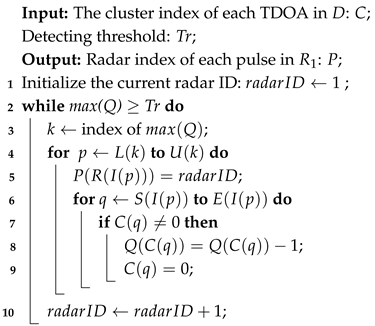
3.3. Pulse Deinterleaving by TDOA Mapping

The mapping relationships among the TDOA index, pulse index, TDOA cluster, and TDOA cluster cardinality are illustrated in Figure 4. The following notations are defined:

• $L\left(k\right)$: This denotes the lower-bound value index of the k-th TDOA cluster. Together with $U\left(k\right)$, they define the range of indices for the TDOA values within the k-th cluster.
• $U\left(k\right)$: It represents the upper-bound value index of the k-th TDOA cluster. The TDOA values within this cluster are indexed from a lower bound to this upper bound.
• $I\left(k\right)$: It represents the original TDOA index before sorting for the k-th element in the sorted TDOA sequence.
• $R\left(k\right)$: For a TDOA index k, $R\left(k\right)$ specifies the corresponding pulse index.
• $C\left(k\right)$: Given a TDOA value with index k, $C\left(k\right)$ indicates the cluster index to which this TDOA value belongs.
• $S\left(k\right)$: Within the TDOA window, for a given pulse index k, $S\left(k\right)$ is the starting TDOA index related to this pulse index.
• $E\left(k\right)$: Within the TDOA window, for a given pulse index k, $E\left(k\right)$ is the ending TDOA index related to this pulse index.
• $Q\left(k\right)$: It denotes the cardinality of the k-th TDOA cluster. In other words, it represents the number of TDOA values in the TDOA cluster with the index k.
• $P\left(k\right)$: This represents the radar index of the pulse with index k, indicating which radar source the pulse originates from.

As depicted in Figure 4, there is a bidirectional correspondence between TDOA clusters and pulse sequences. For any given TDOA cluster, all the TDOAs that are part of this cluster can be uniquely identified. Subsequently, a corresponding set of pulses at the receiver $R_1$ can be determined. In contrast, for any pulses received at $R_1$, the TDOAs related to these pulses can be recognized. Once these TDOAs are identified, the TDOA clusters to which they belong can be unequivocally pinpointed. Based on the analysis in Section 2, the cluster with the largest cardinality is the cluster of Same-Pulse TDOA, which exhibits a one-to-one mapping with the pulse sequence of a certain radar. Therefore, as shown in Algorithm 4, the pulse sequences can be deinterleaved by the mapping deinterleaving algorithm, which is achieved by repeating the following two steps until the quantity of pulses is less than threshold $Tr$. Step 1: Extract the pulse sequence from a certain radar by searching the TDOA cluster with the largest cardinality. Step 2: Prune the TDOAs related to the deinterleaved pulse sequence from the corresponding clusters. The problem of false alarms caused by Same-Source TDOA will be solved as the result of all TDOAs related to the deinterleaved pulse sequence being pruned by Step 2. Since the TDOAs will only be traversed once, the time complexity of the algorithm is $O\left(n\right)$.   

Algorithm 4 Mapping deinterleaving

3.4. Time Complexity Analysis

The proposed pulse deinterleaved method consists of the following three algorithms: the TDOA generating algorithm, SSC-DBSCAN algorithm, and TDOA mapping algorithm. As analyzed in Section 3.1, Section 3.2 and Section 3.3, the time complexity of the TDOA generating algorithm is $O\left(n\right)$, the time complexity of the SSC-DBSCAN algorithm is $O\left(nlogn\right)$, and the time complexity of the mapping deinterleaving algorithm is $O\left(n\right)$. Therefore, the time complexity of the proposed pulse deinterleaved method is $O\left(nlogn\right)$.

4. Simulation and Analysis

4.1. Simulation Settings

A series of simulations are conducted to evaluate the performance of the proposed method. There are 10 radars within the reconnaissance range, and the parameter settings of each radar are shown in

Table 1. Parameters of the radar pulse.

Radar	PRI Modulation	PRI (μs)	RF (MHz)	PW (μs)	PA	Quantity of Pulses	TDOA (μs)
E1	Fixed PRI	493	2300	9	1.2	202	−140.34
E2	Stagger PRI	$513/533/553$	2900∼3050	11	2	187	250.25
E3	Jitter PRI	$620\pm 10\%$	3200∼3300	11	1.5	161	330.63
E4	Fixed PRI	697	2400	9	1.8	143	10.37
E5	Sliding PRI	730∼770	2700	13	1.7	132	−373.12
E6	Fixed PRI	837	2100∼2150	14	1.5	119	151.34
E7	Jitter PRI	1300 ± 10%	3100∼3300	11	1.6	76	−290.27
E8	Fixed PRI	1674	2500	17	1	59	295.47
E9	Stagger PRI	9123/9153/9183	2400	16	1.9	10	−30.44
E10	Fixed PRI	10,055	2500	17	1.5	9	−230.54

. The observation time is $T=0.1$ s and the TDOA window is $[-400\mathsf{\mu }\mathrm{s},400\mathsf{\mu }\mathrm{s}]$ for the ESM system. Based on the typical precision ranges of PDW parameters measured by the ESM system [23,24,26,27], the errors in PDWs are configured as follows. The maximum measurement error of the TOA is ${\sigma }_t=50$ ns, while Gaussian random errors with a mean of 0 and a standard deviation of 1 MHz, 0.1, and 0.15 are applied to the RF, PW, and PA of the pulse, respectively. The simulation was conducted on an i5-6300HQ CPU with a frequency of 2.3 GHz, 8 GB of RAM, and Matlab 2016b.

4.2. Simulation and Analysis of the Quantity Distribution of TDOAs

To verify the correctness of the theoretical analysis on the quantity distribution of TDOAs, this section will cluster TDOAs based on SSC-DBSCAN. The algorithm parameters are set as follows: $e_{rf}=\infty$, $e_{pw}=\infty$, $Eps=100$ ns, $MinPts=0$, $Tr=3$. Since each radar in E1∼E5 represents a typical type of radar, we cluster the TDOA of E1, E2, E3, E4, and E5, respectively. Based on the clustering results, the quantity distribution of each radar’s TDOA is shown in Figure 5a–e.

From Figure 5, it is apparent that the clusters are generated at the Same-Pulse TDOA values of each radar. The cardinality of the cluster is equal to the quantity of the pulses for the corresponding radar, which is consistent with (5). The Same-Source TDOA clusters of all radars are generated, except for E4, since E4 does not meet the generation condition of Same-Source TDOA (6). Regardless of the PRI modulation mode, the cardinality of the Same-Source cluster for each radar is smaller than the cardinality of the Same-Pulse cluster. This is consistent with the analysis in Section 2.2, and it is also the basis of the mapping deinterleaved method.

4.3. Performance Comparison with Other Methods

We conduct a performance comparison with the methods mentioned in [23,24,27] to further verify the superiority of the proposed method. We performed 5000 simulation experiments for each method and calculated the average results under different maximum measurement errors of TOA, ${\sigma }_t$. Since the RF and PW of pulses follow normal distributions, the algorithm in this paper takes three times the standard deviation of the RF and PW as the parameter error range based on the principle of $3\sigma$. The parameters are set as follows: $e_{rf}=6$ MHz, $e_{pw}=0.6\mathsf{\mu }\mathrm{s}$, $Eps=2{\sigma }_p$, $MinPts=3$, $Tr=3$. The simulation results are shown in

Table 2. Simulation results of four deinterleaving methods.

	${\mathit{\sigma }}_{\mathit{t}}$	Proposed	[23]	[24]	[27]
$P_a$	50 ns	99.86%	94.83%	95.99%	99.78%
	100 ns	99.86%	94.84%	95.99%	99.78%
	150 ns	99.87%	94.87%	96.00%	99.80%
	200 ns	99.87%	94.86%	96.00%	99.80%
$P_f$	50 ns	0%	17.70%	17.58%	155.5%
	100 ns	0%	17.73%	17.63%	155.5%
	150 ns	0%	17.56%	17.52%	155.5%
	200 ns	0%	17.58%	17.50%	155.5%
$P_m$	50 ns	0%	4.4%	0%	0%
	100 ns	0%	3.4%	0%	0%
	150 ns	0%	1.2%	0%	0%
	200 ns	0%	1.8%	0%	0%
t	50 ns	0.056 s	2.040 s	1.621 s	0.170 s
	100 ns	0.057 s	2.131 s	1.674 s	0.163 s
	150 ns	0.056 s	2.049 s	1.600 s	0.168 s
	200 ns	0.056 s	2.059 s	1.661 s	0.164 s

, where $P_a$, $P_f$, $P_m$, and t represent the accuracy, false alarm rate, missed alarm rate, and the average running time, respectively [26]. $P_a$, $P_f$, and $P_m$ are defined as

$$\begin{array}{c}\hfill P_a={\displaystyle \frac{N_c}{N}}\\ \hfill P_f={\displaystyle \frac{M_f}{M_r}}\\ \hfill P_m={\displaystyle \frac{M_m}{M}}\end{array}$$

(8)

where N represents the total number of pulses received by the ESM system, $N_c$ is the quantity of pulses that have been correctly deinterleaved, $M_f$ is the quantity of radar sources erroneously reported by the method (non-existent in reality), $M_r$ is the quantity of radar sources reported by the method, M represents the total quantity of radar sources within the detectable range of the ESM system, and $M_m$ is the quantity of radar sources that the method failed to deinterleave.

Table 2 shows that the proposed method has better comprehensive performance compared with other methods, particularly in terms of false alarm rate and running time. The proposed method achieves the maximum deinterleaving accuracy of 99.86% among all methods with a 0% missed alarm rate across varying TOA measurement error conditions. While the maximum measurement error of TOA emerges as the most sensitive parameter for these methods, this result confirms the proposed method’s robust tolerance to environmental parameter variations.

Besides, due to the inability of TDOA windows and PDW constraints to eliminate all Cross-Source TDOAs, a small amount of Cross-Pulse TDOAs with the same value as Same-Pulse TDOAs are clustered into the same group, causing the missorting of pulses and 0.13∼0.14% loss of accuracy in the simulations. The average running time of the proposed method is less than $0.06$ s, which is at least 66% lower than the other three methods. In Refs. [23,24], the histogram of the remaining TDOAs must be recomputed before sorting the radar pulse sequence each time. Similarly, Ref. [27] requires multiple clustering operations to fully sort all radar pulse sequences, leading to an increase in running time. Specifically, the proposed method only clusters the TDOA once throughout the entire process and deinterleaves the pulses based on this clustering result, which significantly reduces the running time compared to existing methods.

In addition, the average false alarm rate $P_f$ of the proposed method is 0%, which is at least 17% lower than the other three methods. Ref. [27] does not eliminate Same-Source TDOAs, leading to a pretty high false alarm rate. Refs. [23,24] present histogram-based TDOA deinterleaved methods and eliminate most Same-Source TDOAs based on a histogram. However, their fixed histogram bins may cause the TDOAs with approximately equal values to be counted into multiple adjacent bins. Each histogram bin exceeding the detection threshold is then falsely identified as a separate pulse sequence, resulting in a high false alarm rate. In contrast, the method proposed employs the density-based clustering algorithm SSC-DBSCAN to resolve these limitations. On the one hand, the soft boundaries constrained by the two parameters, $Eps$ and $MinPts$, prevent the Same-Pulse TDOAs of the same radar from being clustered into different groups. On the other hand, the TDOA mapping algorithm is used to eliminate Same-Source TDOAs based on the clustering results. Therefore, the proposed method achieves a zero false alarm in simulations, which is a significant advancement over existing methods.

4.4. Performance of the Proposed Method Under Different Values of $Eps$

$Eps$ and $MinPts$ are the key parameters of the proposed method. To evaluate the method’s performance across varying $Eps$ values, 5000 simulations were conducted with $Eps$ set to 25 ns, 50 ns, 75 ns, 100 ns, 125 ns, 150 ns, 175 ns, and 200 ns, respectively, while keeping all other parameters unchanged. Figure 6 presents the mean values of $P_a$, $P_f$, and $P_m$ and the running time for the proposed deinterleaving method under different $Eps$ values.

As shown in Figure 6, when $Eps<100$ ns, the method exhibits minor false alarms and missed alarms. Conversely, when $Eps\ge 100$ ns, the method maintains excellent and stable performance as follows: the average accuracy exceeds $99.8\%$, both the false alarm and missed alarm rates remain at $0\%$, and the running time stays below $0.06$ s. This stability arises because the maximum measurement error of TOA is $\pm 50$ ns, leading to a maximum Same-Pulse TDOA error of $\pm 100$ ns. Setting $Eps$ to at least twice the maximum TOA error (100 ns) ensures that all Same-Pulse TDOAs from the same radar are clustered into a single group. Therefore, $Eps$ is recommended to be set as twice the maximum measurement error in practical applications.

4.5. Performance of the Proposed Method Under Different Values of $MinPts$

In order to evaluate the performance of the proposed method at different values of $MinPts$, 5000 sets of simulations are conducted with $MinPt$ ranging from 0 to 10, while other parameters remain unchanged. Figure 7 illustrates the mean values of $P_a$, $P_f$, $P_m$, and the running time for the proposed deinterleaving method under different values of $MinPts$. Figure 8 further details the deinterleaving accuracy for individual radar pulse sequences.

As demonstrated in Figure 7, the proposed method maintains excellent and stable performance when $MinPts\le 8$. The average accuracy exceeds $99\%$, the false alarm rate and the missed alarm rate remain at $0\%$, and the running time stays below $0.06$ s with minimal variation. Besides, the deinterleaving accuracy for individual radar pulse sequences also surpasses $99\%$ when $MinPts\le 8$. In contrast, when $MinPts=9$, the average accuracy of our method decreases, and the average missed alarm rate approaches $10\%$. When $MinPts=10$, the average accuracy of our method continues to decrease, with the average false alarm rate approaching $20\%$. Figure 7 shows that the average accuracy of E9 is approximately $0\%$ when $MinPts=9$ and 10, and the average accuracy of radar E10 is approximately 0 when $MinPts=10$. Combined with Figure 7 and Figure 8, it can be inferred that when $MinPts=9$ and 10, the increase in the missing alarm rate is caused by the missing alarm of radar E9 and E10, as the number of E9 and E10 is relatively small during the observation time. According to Table 1, the number of intercepted pulses of E9 and E10 is 9 and 10, respectively. Therefore, when $MinPts=9$ or 10, the missing alarm of E9 and E10 is caused by $MinPts$ being greater than or equal to the number of intercepted pulses of radar. Based on the above analysis, it can be concluded that when $MinPts$ is less than the number of intercepted pulses from each radar, the proposed method can maintain stable performance. Due to the inability to know in advance the number of pulses intercepted, $MinPts$ can be set to $MinPts\le Tr$ to avoid missed alarms.

5. Conclusions

A novel multi-receiver pulse deinterleaving method based on SSC-DBSCAN and TDOA mapping is proposed in this paper, which aims to effectively deinterleave pulses of various PRI modulation modes. The TDOA of the ESM system can be categorized into Same-Pulse, Same-Source, and Cross-Source TDOA. The distribution features of different types of TDOAs are analyzed to provide the theoretical basis for the proposed method at the start.

The proposed method deinterleave pulses through the following three steps: TDOA extracting, TDOA clustering, and TDOA mapping. In the first step, the Cross-Source TDOAs are reduced through the TDOA window and PDW constraints. Then, an efficient clustering algorithm named SSC-DBSCAN is proposed. By pre-sorting the data and then traversing key points, SSC-DBSCAN realizes TDOA clustering with a low time complexity of $O(nlogn)$. Finally, the TDOA mapping algorithm is proposed, which separates pulses and eliminate Cross-Source TDOAs simultaneously, based on a one-time clustering result. As a result, the false alarm rate has significantly decreased while avoiding repeatedly clustering TDOA.

The results show that compared with other TDOA methods, the running time and the false alarm rate has been decreased by at least $66\%$ and $17\%$, respectively, in cases where performance is slightly better in other aspects. In addition, it is shown that our method is robust, maintaining excellent performance under multiple parameter settings.

References

1. Lang, P.; Fu, X.; Cui, Z.; Feng, C.; Chang, J. Subspace Decomposition Based Adaptive Density Peak Clustering for Radar Signals Sorting. IEEE Signal Process. Lett. 2022, 29, 424–428. [Google Scholar] [CrossRef]
2. Sui, J.; Liu, Z.; Liu, L.; Li, X. Progress in Radar Emitter Signal Deinterleaving. J. Radars 2022, 11, 418–433. [Google Scholar]
3. Zhu, M.; Wang, S.; Li, Y. Model-Based Representation and Deinterleaving of Mixed Radar Pulse Sequences with Neural Machine Translation Network. IEEE Trans. Aerosp. Electron. Syst. 2022, 58, 1733–1752. [Google Scholar] [CrossRef]
4. Mardia, H.K. New techniques for the deinterleaving of repetitive sequences. IEE Proc. F (Radar Signal Process.) 1989, 136, 149–154. [Google Scholar] [CrossRef]
5. Milojević, D.J.; Popović, B.M. Improved algorithm for the deinterleaving of radar pulses. IEE Proc. F (Radar Signal Process.) 1992, 139, 98–104. [Google Scholar] [CrossRef]
6. Xie, M.; Zhao, C.; Zhao, Y.; Hu, D.; Wang, Z. A novel method for deinterleaving radar signals: First-order difference curve based on sorted TOA difference sequence. IET Signal Process. 2023, 17, e12162. [Google Scholar] [CrossRef]
7. Bagheri, M.; Sedaaghi, M.H. A new approach to pulse deinterleaving based on adaptive thresholding. Turk. J. Elec. Eng. Comp. Sci. 2017, 25, 3827–3838. [Google Scholar] [CrossRef]
8. Liu, Y.; Zhang, Q. Improved method for deinterleaving radar signals and estimating PRI values. IET Radar Sonar Navig. 2018, 12, 506–514. [Google Scholar] [CrossRef]
9. Nelson, D.J. Special purpose correlation functions for improved signal detection and parameter estimation. In Proceedings of the 1993 IEEE International Conference on Acoustics, Speech, and Signal Processing, Minneapolis, MN, USA, 27–30 April 1993; Volume 4, pp. 73–76. [Google Scholar]
10. Nishiguchi, K.; Kobayashi, M. Improved algorithm for estimating pulse repetition intervals. IEEE Trans. Aerosp. Electron. Syst. 2000, 36, 407–421. [Google Scholar] [CrossRef]
11. Cheng, W.; Zhang, Q.; Dong, J.; Wang, C.; Liu, X.; Fang, G. An Enhanced Algorithm for Deinterleaving Mixed Radar Signals. IEEE Trans. Aerosp. Electron. Syst. 2021, 57, 3927–3940. [Google Scholar] [CrossRef]
12. Dong, H.; Wang, X.; Qi, X.; Wang, C. An Algorithm for Sorting Staggered PRI Signals Based on the Congruence Transform. Electronics 2023, 12, 2888. [Google Scholar] [CrossRef]
13. Dadgarnia, A.; Sadeghi, M.T. A novel method of deinterleaving radar pulse sequences based on a modified DBSCAN algorithm. China Commun. 2023, 20, 198–215. [Google Scholar] [CrossRef]
14. Kang, K.; Zhang, Y.; Guo, W.; Tian, L. Key Radar Signal Sorting and Recognition Method Based on Clustering Combined PRI transform Algorithm. J. Artif. Intell. Technol. 2022, 2, 62–68. [Google Scholar] [CrossRef]
15. Zhu, M.; Li, Y.; Wang, S. Model-Based Time Series Clustering and Interpulse Modulation Parameter Estimation of Multifunction Radar Pulse Sequences. IEEE Trans. Aerosp. Electron. Syst. 2021, 57, 3673–3690. [Google Scholar] [CrossRef]
16. Dong, X.; Liang, Y.; Wang, J. Distributed Clustering Method Based on Spatial Information. IEEE Access 2022, 10, 53143–53152. [Google Scholar] [CrossRef]
17. Liu, Z.-M.; Yu, P.S. Classification, Denoising, and Deinterleaving of Pulse Streams with Recurrent Neural Networks. IEEE Trans. Aerosp. Electron. Syst. 2019, 55, 1624–1639. [Google Scholar] [CrossRef]
18. Gasperini, S.; Paschali, M.; Hopke, C.; Wittmann, D.; Navab, N. Signal Clustering with Class-Independent Segmentation. In Proceedings of the ICASSP 2020–2020 IEEE International Conference on Acoustics, Speech and Signal Processing (ICASSP), Barcelona, Spain, 4–8 May 2020; IEEE: Piscataway, NJ, USA, 2020; pp. 3982–3986. [Google Scholar]
19. Chen, T.; Yang, B.; Guo, L. Radar Pulse Stream Clustering Based on MaskRCNN Instance Segmentation Network. IEEE Signal Process. Lett. 2023, 30, 1022–1026. [Google Scholar] [CrossRef]
20. Chen, T.; Liu, Y.; Guo, L.; Lei, Y. A novel deinterleaving method for radar pulse trains using pulse descriptor word dot matrix images and cascade-recurrent loop network. IET Radar Sonar Navig. 2023, 17, 1626–1638. [Google Scholar] [CrossRef]
21. Li, W.; Zhang, Z.; Li, H.; Wang, L.; Man, Y. Performance test and evaluation technology for multi-station TDOA location system. Syst.-Eng.-Theory Pract. 2015, 35, 506–512. [Google Scholar]
22. Ren, W.; Hu, D.; Ding, C. New method for TDOA sorting and pairing using TDOAs’ correlation. J. Xidian Univ. 2011, 38, 89–96. [Google Scholar]
23. Ma, S.; Wu, H.; Liu, Z.; Jiang, W. Method for emitter TDOA sorting based on recursive extended histogram. J. Natl. Univ. Def. Technol. 2012, 34, 83–89. [Google Scholar]
24. Liu, Z.; Zhao, Y. Pulse sorting and pairing based on the constrained extended TDOA histogram. J. Xidian Univ. 2019, 46, 102–111. [Google Scholar]
25. Meng, X.-H. Joint sorting algorithm based on direction finding of multiple observation platforms and multi-parameter information. Control Decis. 2016, 31, 160–164. [Google Scholar]
26. Qiu, H.; Zhou, L.; Zhou, Z.; Gu, Y.; Di, C. Multi-Station Sorting Method for Emitter Signal Based on Cloud Model. Acta Electron. Sin. 2022, 50, 2469–2477. [Google Scholar]
27. Jiang, H.; Zhao, C.; Hu, D.; Zhao, Y.; Zhao, Y.; Liu, Z. Real-Time Deinterleaving Algorithm for Single Pulse Signal Based on TDOAs and Multi-parameter Information. Acta Electron. Sin. 2021, 49, 566–572. [Google Scholar]
28. Chen, T.; Wang, T.; Guo, L. Recognition of Pulse Repetition Interval of Multilayer Percetron Network Based on Multi-parameter TDOA Sorting. J. Electron. Inf. Technol. 2018, 40, 1567–1574. [Google Scholar]
Figure 1. Cooperative reconnaissance diagram of an ESM system with two receivers.
Electronics 14 01833 g001
Figure 2. Illustration of the TDOA window and PDW constraints for pulse pairing.
Electronics 14 01833 g002
Figure 3. Diagram of cluster distribution after data ascending.
Electronics 14 01833 g003
Figure 4. The mapping relationships among the TDOA index, pulse index, TDOA cluster and TDOA cluster cardinality.
Electronics 14 01833 g004
Figure 5. Quantity distribution of each radar’s TDOA.
Electronics 14 01833 g005
Figure 6. Pulse deinterleaving results of the proposed method under different values of E p s .
Electronics 14 01833 g006
Figure 7. Pulse deinterleaving results of the proposed method under different values of M i n P t s .
Electronics 14 01833 g007
Figure 8. Deinterleaving accuracy of pulse sequences from each radar across varying M i n P t s values.
Electronics 14 01833 g008